A Graphical Model to Diagnose Product Defects with Partially Shuffled Equipment Data


1
Department of Industrial and Management Engineering, Hanyang University, Ansan 15588, Korea
2
Department of Industrial Engineering and Management, National Taipei University of Technology, Taipei 106, Taiwan
*
Author to whom correspondence should be addressed.
Processes 2019, 7(12), 934; https://0-doi-org.brum.beds.ac.uk/10.3390/pr7120934
Submission received: 26 October 2019
/
Revised: 2 December 2019
/
Accepted: 5 December 2019
/
Published: 8 December 2019
(This article belongs to the Special Issue Fault Detection and Process Diagnostics by Using Big Data Analytics in Industrial Applications)
Abstract
:The diagnosis of product defects is an important task in manufacturing, and machine learning-based approaches have attracted interest from both the industry and academia. A high-quality dataset is necessary to develop a machine learning model, but the manufacturing industry faces several data-collection issues including partially shuffled data, which arises when a product ID is not perfectly inferred and yields an unstable machine learning model. This paper introduces latent variables to formulate a supervised learning model that addresses the problem of partially shuffled data. The experimental results show that our graphical model deals with the shuffling of product order and can detect a defective product far more effectively than a model that ignores shuffling.
1. Introduction
The diagnosis of product defects is essential for improving productivity in manufacturing. The task involves deciding whether a product is defective, given product-related information (e.g., image of completed products, and equipment data). Thanks to large volumes of data collected from factories and the advent of machine learning algorithms, data-driven defect diagnosis is receiving increasing attention from both the industry and academia. Data-driven defect diagnosis involves the development of a classifier by using a training dataset that consists of for , where is a feature vector and is the label of product , as well as using the classifier to diagnose product defects.
Data-driven defect diagnosis uses either a feature vector (i.e., input data), such as completed product data (e.g., the image and specification of products) or equipment (e.g., command and sensor) data. Equipment data, including the manufacturing process for each product, can be used to diagnose defects before a product is produced. For example, Manco et al. [1] applied outlier detection to predict door failures on metro trains, and Khalastchi et al. [2] proposed a hybrid approach to detect faults in robotic systems based on sensor readings, commands, and feedbacks from actuators. Song and Shi [3] proposed a quality-supervised double-layer method to detect quality-related faults in which the first layer uses principal component analysis (PCA) to detect the fault and the second layer finds the key variable orthogonal weight of the fault from the PCA. Fakhfakh et al. [4] developed a mathematical model for on-line fault diagnosis, resulting in the schedule delays of a flexible manufacturing system to minimize the total delays caused by faults. They also developed a constraint programming technique to solve this mathematical problem.
Multi-source data fusion that combines or merges data from multiple sources (e.g., multiple sensors and two or more machines) is necessary for realistic defect diagnosis with equipment data [5]. It can be categorized as signal-level, feature-level, or decision-level fusion [6]. Among them, feature-level fusion extracts feature vectors from each data point and merges them based on product ID. It is used primarily to combine a dataset to train a defect diagnosis model [7,8].
However, multi-source data fusion cannot always be effectively conducted due to imperfections, correlations, inconsistency, disparateness, etc. [9]. In many cases (e.g., a specific subprocess such as milling in the manufacturing process), a product ID cannot be attached until the production process is finished. In such cases, inferring a product ID should be conducted first. However, it cannot be perfectly inferred when there are one or more workstations such that (1) two or more independent parallel machines reside in a workstation, (2) the processing time of each machine is variable, and (3) workstations cannot be observed from the outside due to safety issues. When equipment data are partially shuffled, there can be no guarantee that a record in data merged by feature-level fusion will indicate a product. We propose a graphical model to diagnose product defects with partially shuffled equipment data. The proposed graphical model calculates the probabilities that products are shuffled and the likelihood that a product is defective by considering the shuffling probability.
To the authors’ best knowledge, this is the first study to address the real and common manufacturing situation in which each product cannot be perfectly traced because merged equipment data based on product IDs may be partially shuffled. This study proposes a simulation method to calculate the probability that product order is shuffled at each workstation based on production-line analysis. The method also includes the calculation of the maximum shuffling range at workstation and probability, , of two products are shuffled with shuffling range . It also proposes a graphical model to diagnose product defects with partially shuffled equipment data with a consideration of product shuffling based on .
Section 2 of this paper describes the problem in detail, focusing on the situation in which partially shuffled equipment data are merged from multiple data sources. Section 3 develops a graphical model to diagnose defects with partially shuffled equipment data through three phases: (1) production-line analysis with simulation, (2) graphical model design, and (3) graphical model inference. Section 4 provides an example of a numerical application of the proposed graphical model, and Section 5 suggests future research directions.
2. Problem Description
Suppose there are serial workstations and that a product must visit each machine at every workstation to be completed. More formally, let product be processed by machine at workstation from time to . The feature for product at workstation , is , where is the feature value collected from machine at workstation at time and means time a unit time elapse (e.g., second and millisecond) after . By expanding the problem to every product and every workstation , a defect diagnosis dataset, can be generated in which and are feature vector and a label of product , respectively.
The problem is to train a classifier with training records and diagnose whether a given product is defective by using the trained classifier. It is a general approach to diagnose defects by using machine learning. However, this approach cannot be employed when some product-processing orders are partially shuffled and the shuffled orders are not known.
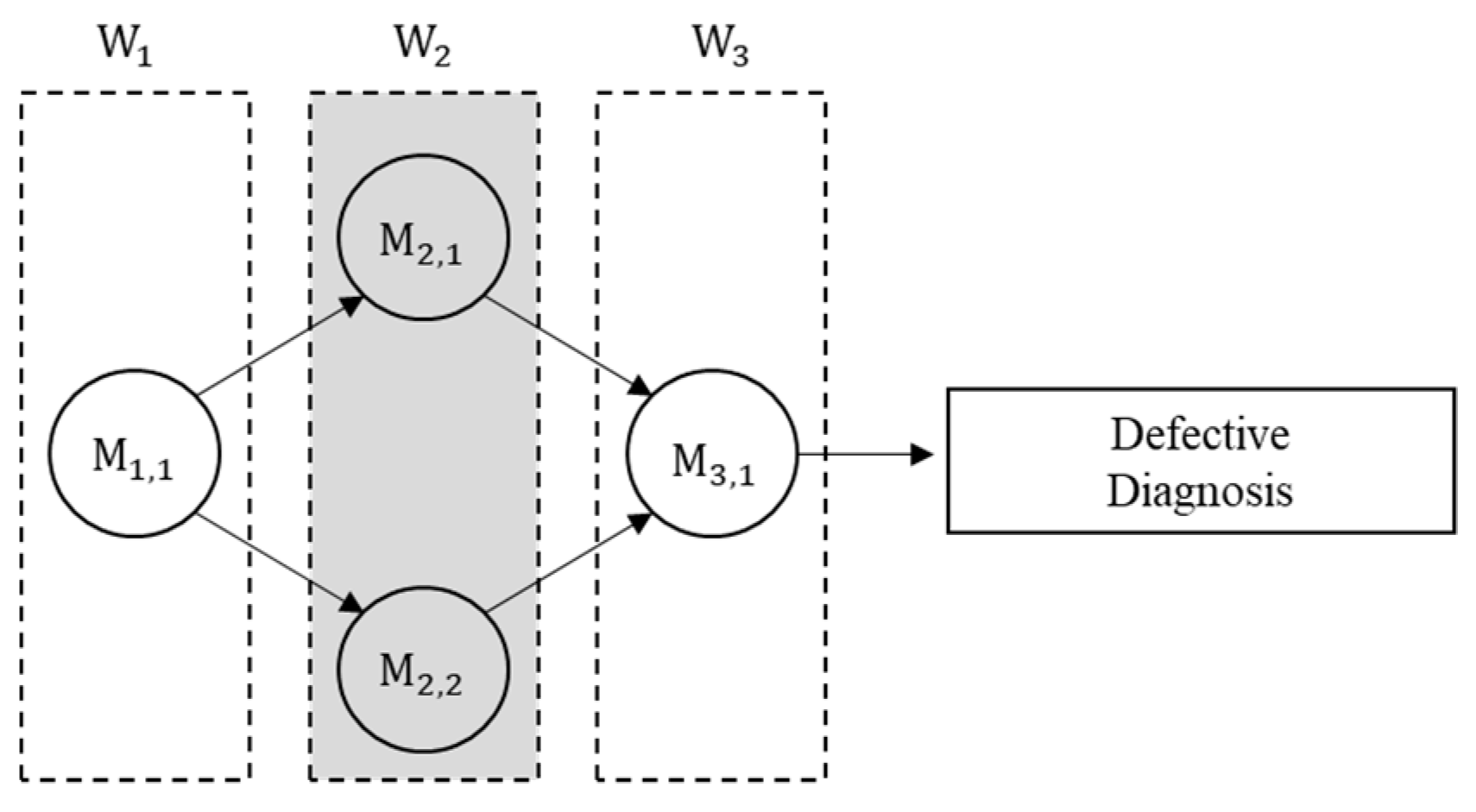
Consider a production line that consists of three workstations (, , ) where product orders maybe shuffled and shuffled orders are not perfectly inferred in because the workstation includes two parallel machines whose processing times are not constant and cannot be observed from outside, as illustrated in Figure 1. The circle indicates a machine, and the dotted rectangle indicates a workstation. Defect diagnosis for each product is conducted after the product is processed by .
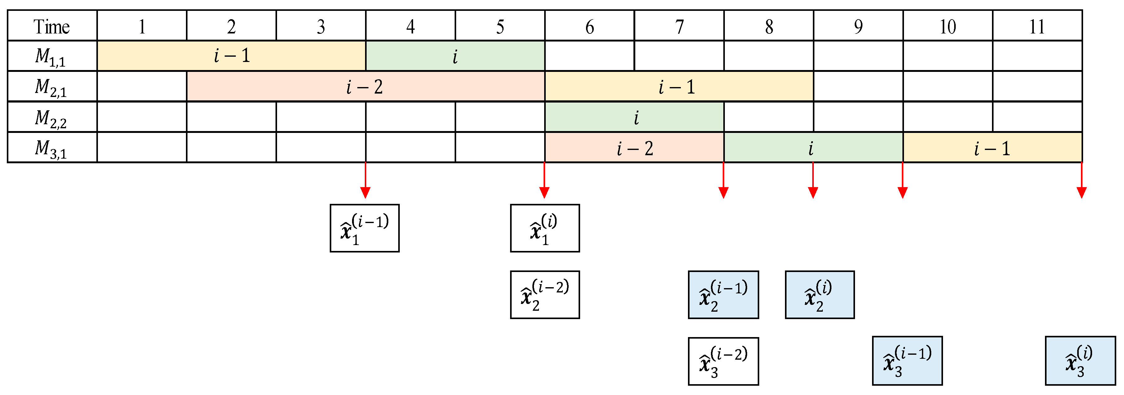
Suppose there are two products with following the sequence and . Suppose also that product enters ahead of product , but product enters after product . This situation can be illustrated in a Gantt chart (Figure 2), in which the arrow, rectangle, and colored rectangle denote the time to extract data, observed data, and shuffled observed data, respectively.
As seen in Figure 2, equipment data for product are a concatenation of ’s data during [1,3], ’s data during [6,8], and ’s data during [10], and equipment data for product is a concatenation of ’s data during [4,5], ’s data during [6,7], and ’s data during [8,9]. One cannot know which product is processed by machines and in , because this workstation is not observed; one can only know if each machine is busy or idle. It is therefore impossible to identify which product is released at time 9 from . In this situation, the feature vector for product is not , but , which affects the training of the classifier . In this paper, we call the observed feature vector for product , and we called the equipment data collected for each product partially shuffled data.
3. Proposed Graphical Model
In this section, we construct a graphical model to diagnose defects with partially shuffled equipment data through three phases: (1) production-line analysis with simulation, (2) graphical model design, and (3) graphical model inference. In the first phase, we characterize the partially shuffled data by means of the shuffling probabilities saved in matrix . In the second phase, latent variables are introduced to design a graphical model structure. In the third phase, probabilistic supervised models for defect detection are trained, and an expectation of probability that a product is defective given the observed feature vector is calculated using the graphical model.
3.1. Production-Line Analysis with Simulation (Characteristics of Shuffled Data)
Let each and indicate the arrival order and completion order of product at workstation . In the absence of shuffling, . If shuffling exists, for some . Let us define the range of shuffling as for product . We can expect that the actual completed product is either the or arriving product. Here, is regarded as a random variable.
Let denote the probability of a shuffle with a range of at workstation , which is formally expressed as:
where means that products arrive between the and arrival times at workstation , and implies that either or products are completed between the and completion at workstation . That is, the arrived product may not be the completed product at the workstation because some products are completed faster or slower than expected. Maximum shuffling range at workstation is calculated as , and is defined for .
Even though plays an important role in developing the graphical model, it is not possible to analytically calculate it when the range of is wide because there are many machines whose processing times are variables. However, we adopted a simulation method that could estimate . The first step is to generate simulated data that consist of simulated production routes for products. Let be the processing route of simulated product , which is a tuple of the machine, start time of processing, and the end time of processing at each workstation:
where , , and indicate the machine that processes product , its start time, and its end time (release time) at workstation , respectively.
A processing route generation algorithm is presented as Algorithm 1. It repeats (1) randomly selecting one of the idle machines to process a product at a workstation, (2) sampling processing time from the distribution of the selected machine’s processing time, (3) calculating the start and end time of the selected machine for the product, and (4) updating the busy/idle status of the selected machine for every product and workstation.
| Algorithm 1 Product Route Generation Algorithm | ||
| Input | , , for all , | |
| Procedure | 01 | Initialize as 1 for all |
| 02 | Initialize as 1 | |
| 03 | For do { | |
| 04 | For do { | |
| 05 | While do {Increase by 1} | |
| 06 | ||
| 07 | ||
| 08 | ||
| 09 | ||
| 10 | for }} | |
| Output | for | |
A specific explanation of Algorithm 1 follows. Every machine’s state for all is initialized as idle (Line 01), and the time is also initialized (Lines 01–02). Product is simulated (Lines 04~10): If there is no idle machine in workstation at , then is increased by 1 until one or more machines become idle (Line 05); the product waits for processing when there is no idle machine. This product then enters a randomly selected idle machine in workstation (Line 06), and the start time for processing the product is set to (Line 07), and the processing time is sampled from its probability distribution (Line 8). The processing time determines the end time of processing product . (Line 09), and the selected machine’s state becomes busy (Line 10).
Using for , obtained from Algorithm 1, we can calculate in Equation (1). First, we calculate and . based on and for all , respectively. Then, we obtain the estimate of from the ratio of pairs that satisfies among those .
3.2. Graphical Model Design (Graphical Model for Shuffled Data)
We can introduce a latent variable to indicate the completed product at each workstation. For example, if , then the 7th completed product at workstation is the one that has entered into that workstation as the 9th. Actually, is unknown if workstation is unobservable, but there can be only one , such that . By introducing these latent variables, we can develop a graphical model that represents the relationships between all and values, and an inference to defect diagnosis is possible.
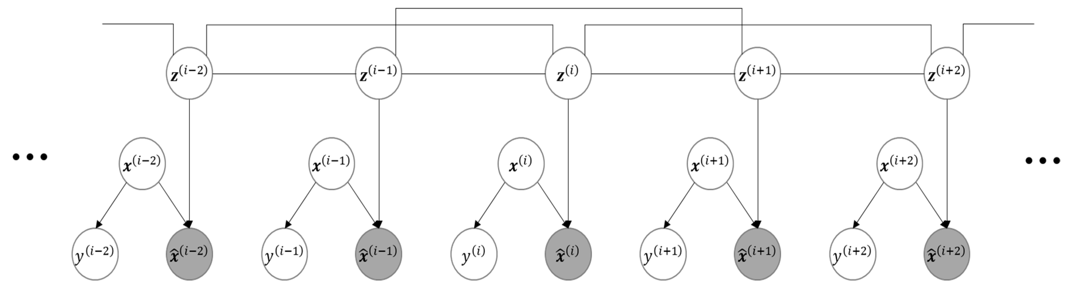
An exemplary structure of graphical model can be given with the help of latent variable , as presented in Figure 3 in the case .
In this figure, shaded circles indicate observable variables, while the others are unobservable. In general, node is connected to because the variable mathematically affects , , …, , and .
With the help of the graphical structure, given can be expressed as:
can be then inferred from and for as:
where is 1 if the condition is satisfied, and 0, otherwise.
3.3. Inference (Defect Diagnosis)
The objective of this paper was to calculate the probability, that product is defective given its feature vector, which may be calculated by a probabilistic supervised model such as logistic regression. However, it cannot be directly obtained because is unobservable, unlike the situation to which a supervised learning model is applied. Thus, we expanded by means of the designed graphical model structure to consider all possible situations in which is distributed in for as:
Now, each part of the right-hand side of Equation (5) can be calculated.
(i) Calculation of
in Equation (5) can be calculated using from the production-line analysis in Section 3.1. When (when there is no partial shuffling), then for all . In this case, equals , implying that is directly calculated from a probabilistic supervised model because . When , a conditional distribution of given can be obtained.
’s distribution can be obtained recursively using Equations (6) and (7).
(ii) Calculation of
This probability is obtained by a supervised machine learning model with a training dataset composed of , i.e., the observed feature vector for product and its label. Specifically, is the feature collected at workstation ; is 1 if the product is defective, and is 0 otherwise. Note that we do not know the exact value of , and it cannot be guaranteed that because of possible shuffling. Instead, we utilized the value of the latent variable to compose a dataset to train the model.
All terms of in the condition part of the probability vanish, except the one that satisfies . Therefore, only those observed feature vectors where are required. This implies the feature vectors used for learning each model are determined by the distribution of . As an example, suppose that can take either , or when the shuffle range is . When or , is used as a feature set, but when , then the feature set is .
4. Numerical Example
This section provides a numerical example to apply the proposed model. In addition, the classification performance of the defect diagnosis is compared between our model, which takes the possibility of shuffling of product order into consideration, and the model that ignores it and assumes for all values of . An F1 score, harmonic mean of the precision and recall, was employed as the classification performance measure to consider both cost of false positives (FPs) and false negatives (FNs). FN cost occurs when an actual defective product is not detected, and this cost covers selling defective products such as customer claim and safety accidents (note that the addressed product is a brake disc, which is extremely safety-critical). FP cost occurs when a normal product is detected as defective, and this cost covers the costs of re-check, re-work, or disposal. Even though FN cost is much greater than FP cost, considering only one cost makes a classifier biased, so we employed an F1 score of 4.1. Line data
We generated an illustrative dataset by referring to a disk-brake processing line of a large-sized auto parts company in Korea for this numerical example’s purpose. The generated data are very similar to the real data except for machine specifications and related parameters. Even though the data are artificial, we believe that the research result can be effectively applied to the real production field when a possible shuffle of production data exists because the main idea and methodology of the research focus on data-shuffling and its effect on the detection of defectives.
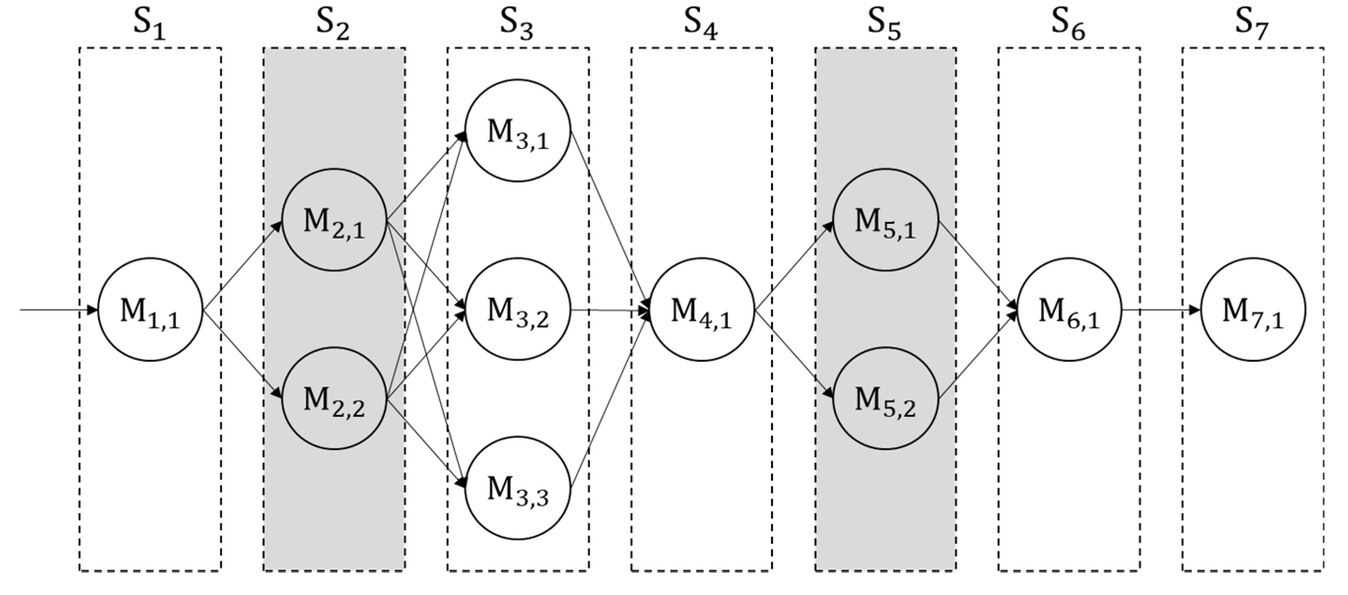
The processing line consists of seven workstations (, , , ) including rough grinding, drilling, and tapping. Figure 4 illustrates the processing line, where a circle, a rectangle, and a colored rectangle denote a machine, a workstation, and a workstation that is not observable, respectively.
As seen in this figure, , , and are composed of parallel machines, and the others include a single machine. We assumed that when a machine is abnormal the products processed by it are all defective.
Table 1 shows machine specifications, including probability density functions, of processing times and sensor values attached to each machine in normal and abnormal states. denotes a normal distribution with mean and standard deviation , and denotes an exponential distribution with mean . The numbers were all created artificially for the purpose of illustration.
4.1. Production-Line Analysis
One million simulated products were generated using Algorithm 1 to estimate partially shuffling probability . The result is summarized in Table 2.
With Table 2 and Equations (6) and (7), we can obtain a probability distribution of . For example, if we calculate the probability that the product arrives at Workstation (1), and overtakes the 77th product at Workstation (2), and is overtaken by two products at Workstation (3) and keeps its order afterward, then it is given by as:
overtaken by two products at Workstation (3) and keeps its order afterward. The probability is then given by:
4.2. Feature Data
A total of values of were generated for all (i.e., ), and they were artificially shuffled to get the observed feature values, . Product could then be expressed as a concatenation of the machine sequence, start and end times, machine state, feature vector, and label as follows:
where represents the feature of statistical values, including variance, skewness, mean, kurtosis, and median extracted from sensor values of the machine processing the product at workstation [10], and indicates machine state (i.e., 0: normal or 1: abnormal). is the label (i.e., whether product is defective or not), calculated as . The number of defective products was 2,136; that is, the defective ratio during that period was 2.136%.
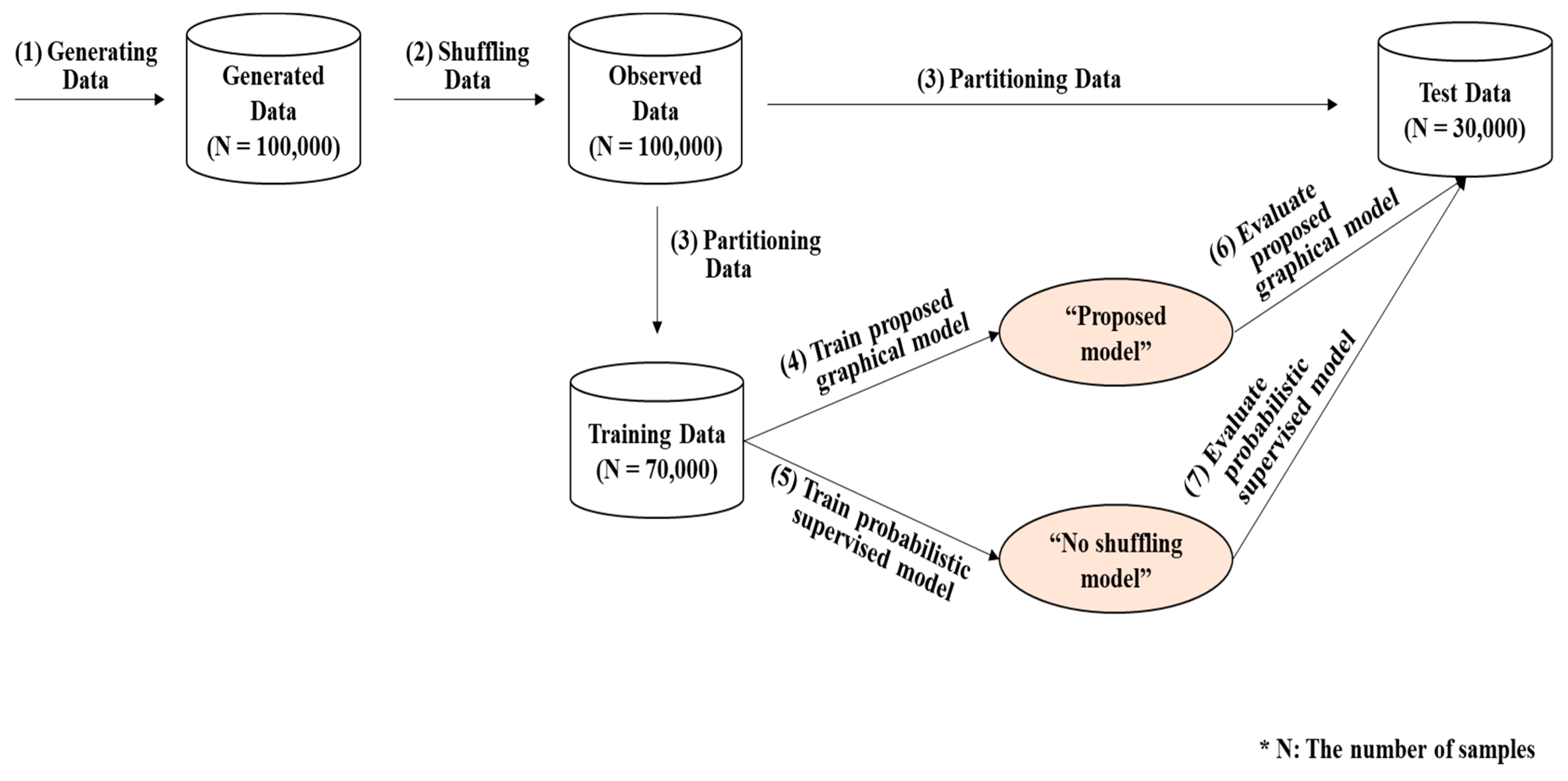
Among the 100,000 values of , randomly chosen values were used to train the proposed graphical model, as well as the one that ignores shuffling of product order. The remaining 30,000 values were reserved for the test of the two models.
4.3. Defect Diagnosis Result
A logistic regression model was employed as a classifier because it is one of the simplest probabilistic classifiers. Other probabilistic classification models may yield similar results. We compared the classification performance between our model and the model that classified the product without consideration of possible shuffling. The proposed model considered the probability that the feature values were shuffled among the products when classifying the product, but the other, “no shuffling,” model assumed the order of collection of feature values was the same as that of the production. The preparation procedure for the dataset to be used for comparison is depicted in Figure 5.
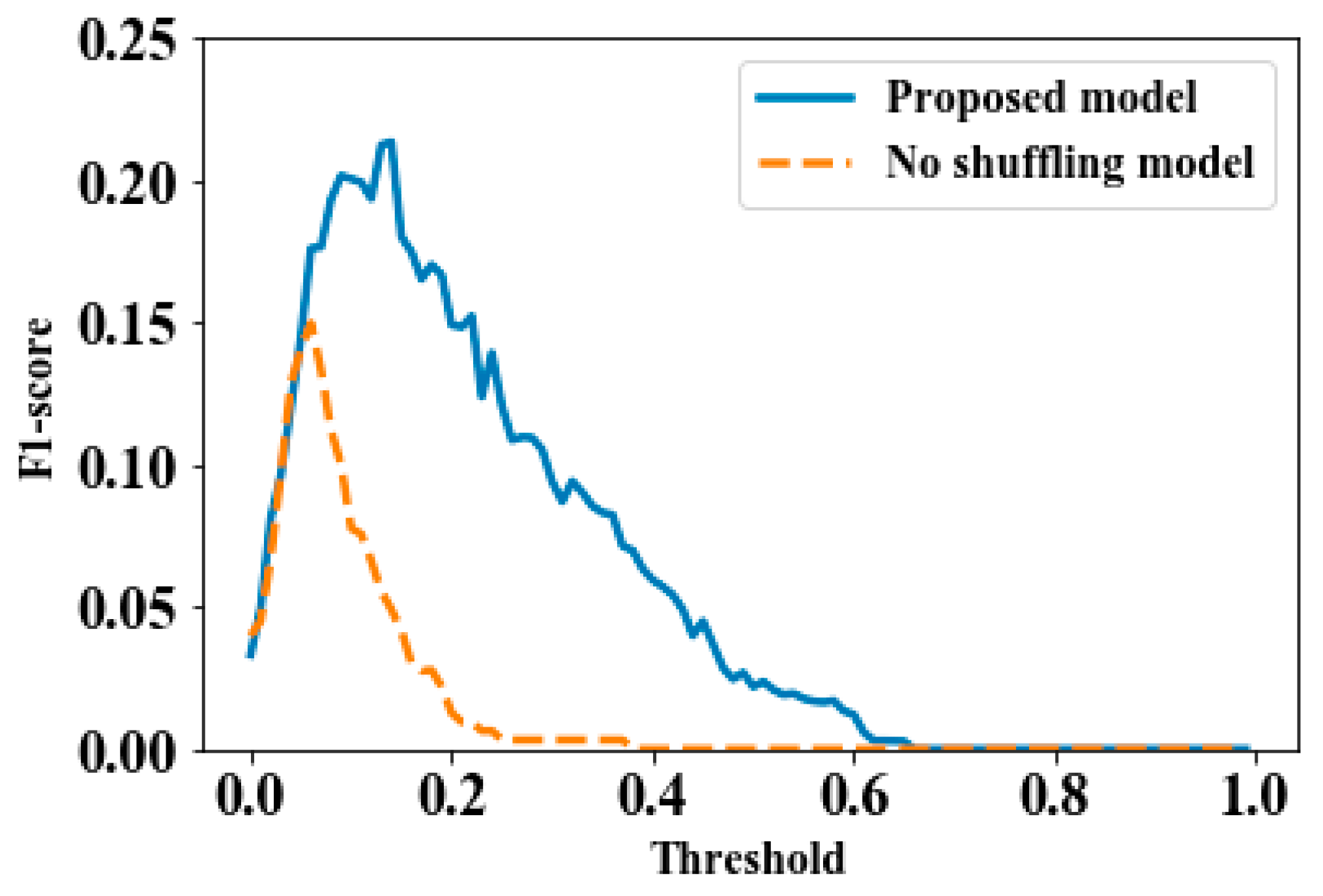
Figure 6 shows the F1 scores of the proposed model and no shuffling model according to various cutoff values of threshold . The model decided whether a product was defective if .
From Figure 6, we can see that the proposed model produced a much higher F1 score over all thresholds. This implies that our graphical model dealt with the shuffling of product order and could detect a defective product far more effectively than a model that ignores shuffling. As a result, one can expect an improved classification result by considering the shuffling when some workstations are unobservable from the outside and the shuffling of product order is expected. When the threshold was small, i.e., under , then the F1 scores of the two models were almost identical, which was expected because both models tried to judge almost all products as defective. Another implication is that the best performance of the “no shuffling” model appeared when the cutoff threshold was near , while the proposed model’s performance was the best when . Therefore, the proposed model was less likely to produce a false alarm (classifying the non-defective as falsely defective) than the “no shuffling” model.
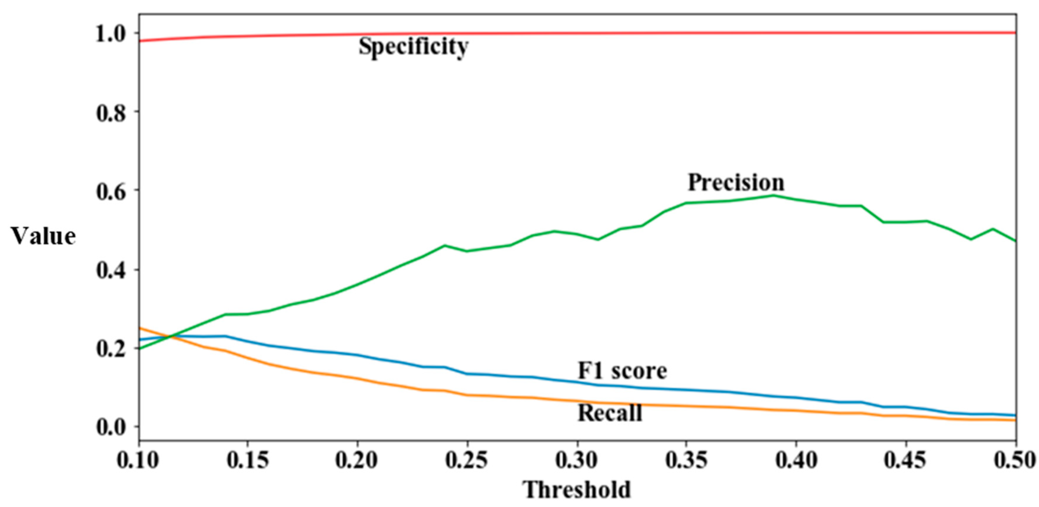
Figure 7 shows values of the F1 score, recall, precision and specificity of the proposed model for the range of . As seen in this figure, the specificity was close to 1 irrespective of , implying that most non-defective products were diagnosed as non-defective (i.e., negative), which was natural because the number of negative records was much greater than the number of positive records. Precision increased as got higher, while recall decreased. The F1 score was more affected by recall than precision because of very small values of recall. From this analysis, the following implications are drawn: First, specificity may not be a proper measure for defective diagnosis when classes are imbalanced. Second, precision and recall show the opposite trend as increases, implying that using only one of them may lead to wrong decision. Specifically, a classifier that determines most records as positive will get higher recall, and the precision of a classifier that regards most records as negative tends to be bigger. Since the F1 score of a highly imbalanced class dataset tends to show a similar trend to recall, a classifier which is not biased to negative class such as a naïve Bayes classifier with uniform prior can be suggested to reduce both misclassification costs.
5. Conclusions
This paper addresses a realistic data quality problem of manufacturing equipment data when developing a product-defect diagnosis model—the partially shuffled data problem. Each record should correspond to a product in order to develop a proper defect diagnosis model, but most records in partially shuffled data do not correspond with a product. This problem results from one or more unobservable workstations that consist of parallel machines. One alternative may be to omit those features that may be partially shuffled if those workstations that produce partially shuffled data are near the end of the manufacturing process. However, if one or more of these workstations is near the front of the process, such as in the numerical example of this paper, omitting features obviously yields a very poor classifier with insufficient feature vector. This is because all the features collected from the workstations followed by that shuffling workstation may be possibly shuffled, and, therefore, we have to remove all features from then on. Thus, omitting features from the workstations cannot recover the shuffle of other features.
Therefore, this paper presents a probabilistic graphical model to diagnose product defects by considering the probabilities that product orders are partially shuffled. The graphical model was designed by means of a production-line analysis, and it was trained by partially shuffled data. From the numerical example, we verified that the graphical model exhibited a similar performance to a classifier trained by data that were not shuffled.
For future research, we will expand the graphical model to diagnose defects in products where the manufacturing sequence of some products varies due to machine breakdown, reworking, and other factors. In addition, we can apply this model to other fields such as traffic management and bio-informatics. Additionally, in order to enhance the model’s diagnosis accuracy as well as to improve its computational efficiency, it will be necessary to develop a proper method for extracting critical features with a shuffling strategy.
Author Contributions
Author contributions are as follows: data curation, D.S.; funding acquisition, S.H.; investigation, G.A. and D.S.; methodology, G.A. and S.H.; project administration, S.H. and D.S.; software, G.A.; validation, G.A.; writing—original draft, G.A.; writing—review and editing, S.H., D.S., and Y.-J.P.
Funding
This work has supported by the National Research Foundation of Korea (NRF) grant funded by the Korea government (MSIT) (2019R1A2C1088255).
Conflicts of Interest
The authors declare no conflict of interest.
Nomenclature
| Indices | |
| Product index, | |
| Workstation index, | |
| Machine index, | |
| Time index, | |
| Simulated product index, | |
| Shuffle range index, | |
| Production Line-Related Terms | |
| Workstation | |
| Machine at workstation | |
| Probability distribution function of ’s processing time | |
| Probability that processing orders of two products, where products are released between their release time at workstation , are switched at workstation | |
| Machine that processes product at workstation | |
| Start time of processing of product at | |
| Processing time of product by | |
| Completion time of processing of product by , | |
| Arrival order of product at workstation | |
| Completion order of product at workstation | |
| Binary variable indicating is idle at , | |
| Model-Related Terms | |
| Feature vector for product , | |
| Time-series data collected from machine at workstation , | |
| Label of product , | |
| Observed feature vector for product | |
| Classifier to diagnose whether each product is defective or not | |
| Latent variable of actual product whose data is collected as | |
References
- Manco, G.; Ritacco, E.; Rullo, P.; Gallucci, L.; Astill, W.; Kimber, D.; Antonelli, M. Fault detection and explanation through big data analysis on sensor streams. Expert Syst. Appl. 2017, 87, 141–156. [Google Scholar] [CrossRef]
- Khaleghi, B.; Khamis, A.; Karray, F.O.; Razavi, S.N. Multisensor data fusion: A review of the state-of-the-art. Inf. Fusion 2013, 14, 28–44. [Google Scholar] [CrossRef]
- Song, B.; Shi, H. Fault detection and classification using quality-supervised double-layer method. IEEE Trans. Ind. Electron. 2018, 65, 8163–8172. [Google Scholar] [CrossRef]
- Fakhfakh, O.; Toguyeni, A.; Korbaa, O. On-line fault diagnosis of FMS based on flows analysis. J. Intell. Manuf. 2018, 29, 1891–1904. [Google Scholar] [CrossRef]
- Ma, Z.; Marchette, D.J.; Priebe, C.E. Fusion and inference from multiple data sources in a commensurate space. Stat. Anal. Data Min. 2012, 5, 187–193. [Google Scholar] [CrossRef] [Green Version]
- Hall, D.L.; Llinas, J. An introduction to multisensor data fusion. Proc. IEEE 1997, 85, 6–23. [Google Scholar] [CrossRef] [Green Version]
- Chen, Z.; Li, W. Multisensor feature fusion for bearing fault diagnosis using sparse autoencoder and deep belief network. IEEE Trans. Instrum. Meas. 2017, 66, 1693–1702. [Google Scholar] [CrossRef]
- Vazifeh, M.R.; Hao, P.; Abbasi, F. Fault diagnosis based on multikernel classification and information fusion decision. Comput. Technol. Appl. 2013, 4, 404–409. [Google Scholar]
- Khalastchi, E.; Kalech, M.; Rokach, L. A hybrid approach for improving unsupervised fault detection for robotic systems. Expert Syst. Appl. 2017, 81, 372–383. [Google Scholar] [CrossRef]
- Safizadeh, M.S.; Latifi, S.K. Using multi-sensor data fusion for vibration fault diagnosis of rolling element bearings by accelerometer and load cell. Inf. Fusion 2014, 18, 1–8. [Google Scholar] [CrossRef]
Figure 1.
Example to illustrate processing orders that can be partially shuffled.

Figure 2.
Gantt chart describing when product orders are shuffled.

Figure 3.
Structure of the graphical model (Case: ).

Figure 4.
Layout of a disk-brake processing line in the numerical example.

Figure 5.
Preparation procedure for the dataset to be used for comparison.

Figure 6.
Defect diagnosis result: F1 scores of the proposed model and no shuffling model.

Figure 7.
Performance measures of the proposed model according to threshold.


Table 1.
Machine specifications of the example.
| Machine | Processing Time | Probability That the Machine Is Abnormal | Sensor Values | |
|---|---|---|---|---|
| At Normal State | At Abnormal State | |||
| 0.001 | ||||
| 0.005 | ||||
| 0.003 | ||||
| 0.010 | ||||
| 0.001 | ||||
| 0.001 | ||||
| 0.001 | ||||
Table 2.
Partially shuffling probability matrix of the numerical example.
| 0 | 1 | 2 | 3 | 4 | 5 | 6 | 7 | 8 | ||
|---|---|---|---|---|---|---|---|---|---|---|
| Work-Station | 1 | 1.0000 | 0.0000 | 0.0000 | 0.0000 | 0.0000 | 0.0000 | 0.0000 | 0.0000 | 0.0000 |
| 2 | 0.6212 | 0.2272 | 0.0901 | 0.0360 | 0.0151 | 0.0063 | 0.0025 | 0.0010 | 0.0004 | |
| 3 | 0.7254 | 0.1808 | 0.0618 | 0.0207 | 0.0072 | 0.0026 | 0.0010 | 0.0003 | 0.0001 | |
| 4 | 1.0000 | 0.0000 | 0.0000 | 0.0000 | 0.0000 | 0.0000 | 0.0000 | 0.0000 | 0.0000 | |
| 5 | 0.8504 | 0.1204 | 0.0229 | 0.0050 | 0.0010 | 0.0003 | 0.0000 | 0.0000 | 0.0000 | |
| 6 | 1.0000 | 0.0000 | 0.0000 | 0.0000 | 0.0000 | 0.0000 | 0.0000 | 0.0000 | 0.0000 | |
| 7 | 1.0000 | 0.0000 | 0.0000 | 0.0000 | 0.0000 | 0.0000 | 0.0000 | 0.0000 | 0.0000 | |
© 2019 by the authors. Licensee MDPI, Basel, Switzerland. This article is an open access article distributed under the terms and conditions of the Creative Commons Attribution (CC BY) license (http://creativecommons.org/licenses/by/4.0/).
Share and Cite
MDPI and ACS Style
Ahn, G.; Hur, S.; Shin, D.; Park, Y.-J. A Graphical Model to Diagnose Product Defects with Partially Shuffled Equipment Data. Processes 2019, 7, 934. https://0-doi-org.brum.beds.ac.uk/10.3390/pr7120934
AMA Style
Ahn G, Hur S, Shin D, Park Y-J. A Graphical Model to Diagnose Product Defects with Partially Shuffled Equipment Data. Processes. 2019; 7(12):934. https://0-doi-org.brum.beds.ac.uk/10.3390/pr7120934
Chicago/Turabian StyleAhn, Gilseung, Sun Hur, Dongmin Shin, and You-Jin Park. 2019. "A Graphical Model to Diagnose Product Defects with Partially Shuffled Equipment Data" Processes 7, no. 12: 934. https://0-doi-org.brum.beds.ac.uk/10.3390/pr7120934
Note that from the first issue of 2016, this journal uses article numbers instead of page numbers. See further details here.