Accelerating Biologics Manufacturing by Upstream Process Modelling

Abstract

Intensified and accelerated development processes are being demanded by the market, as innovative biopharmaceuticals such as virus-like particles, exosomes, cell and gene therapy, as well as recombinant proteins and peptides will possess no available platform approach. Therefore, methods that are able to accelerate this development are preferred. Especially, physicochemical rigorous process models, based on all relevant effects of fluid dynamics, phase equilibrium, and mass transfer, can be predictive, if the model is verified and distinctly quantitatively validated. In this approach, a macroscopic kinetic model based on Monod kinetics for mammalian cell cultivation is developed and verified according to a general valid model validation workflow. The macroscopic model is verified and validated on the basis of four decision criteria (plausibility, sensitivity, accuracy and precision as well as equality). The process model workflow is subjected to a case study, comprising a Chinese hamster ovary fed-batch cultivation for the production of a monoclonal antibody. By performing the workflow, it was found that, based on design of experiments and Monte Carlo simulation, the maximum growth rate µ_max exhibited the greatest influence on model variables such as viable cell concentration X_V and product concentration. In addition, partial least squares regressions statistically evaluate the correlations between a higher µ_max and a higher cell and product concentration, as well as a higher substrate consumption.

1. Introduction

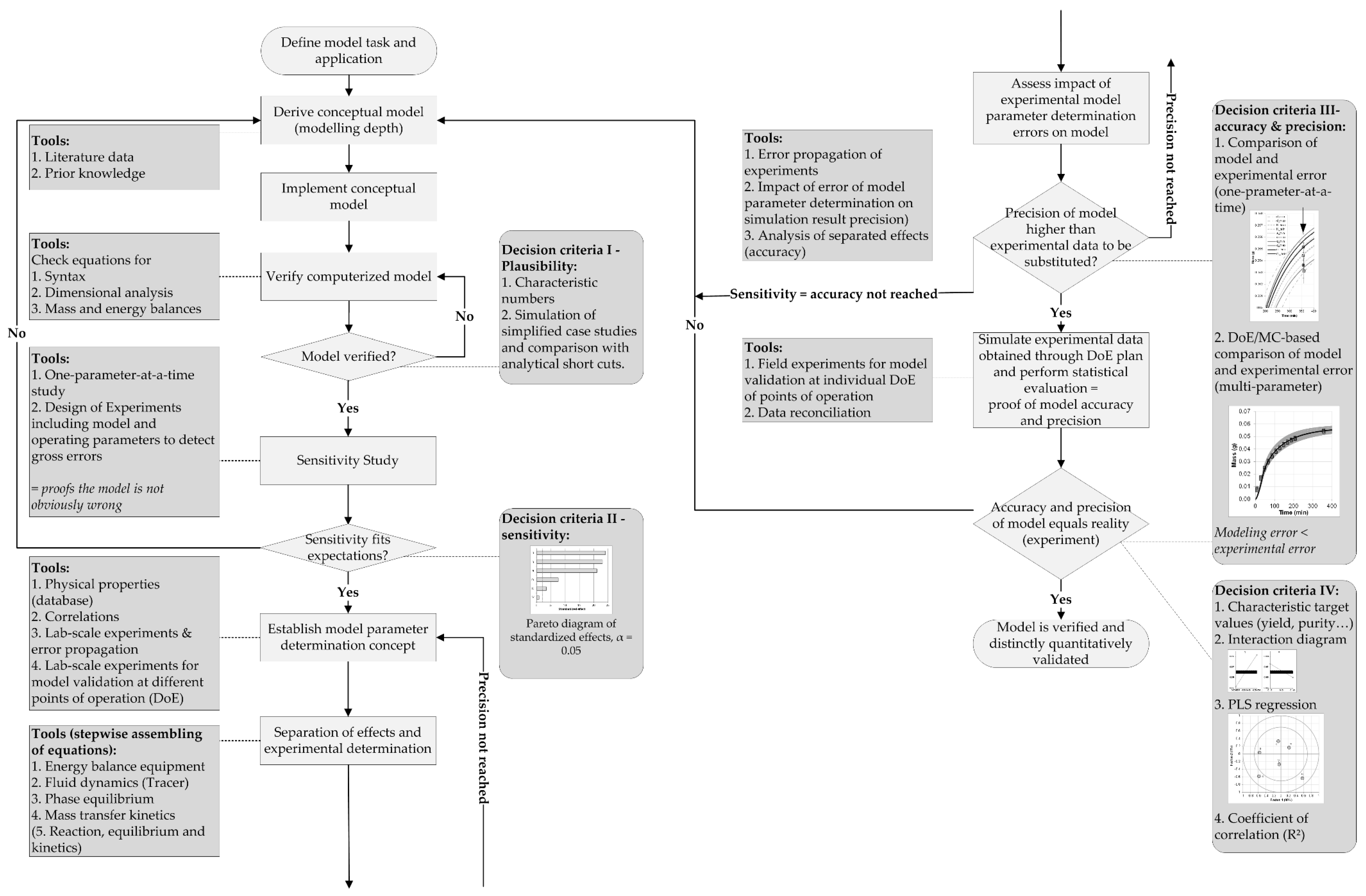
The process analytical technology (PAT), which was initiated by the Food and Drug Administration (FDA) in 2004, is a key-enabling technology for quality-by-design (QbD) process development approaches [1,2,3]. The steadily increasing demand for process robustness, as well as for reducing cost of goods (COGs) and batch variability, requires intensified processes, detailed process understanding, and control [4]. Therefore, the PAT initiative aims at measuring, analyzing, monitoring, and ultimately controlling all important attributes of the process [1,5,6,7]. Bioprocess (i.e., cultivation in batch, fed-batch, and continuous operational mode) monitoring includes process variables such as (viable) cell, substrate, metabolite, and product concentration, as well as product quality and impurities. These target variables depend on state variables such as pH, dissolved oxygen (pO₂), and temperature, providing suitable cultivation conditions [8]. Furthermore, state variables are controlled via process variables such as the addition of base, acid, substrates, and salts, as well as the adjustment of stirrer rates, air flow, and heating/cooling temperatures [9]. The ability for measurement, analysis, monitoring, and controlling of variables, preferably online, is strongly dependent on the state (i.e., physical, chemical, biological), the variable itself, and available sensor techniques [2,10]. An online estimation of difficult to measure variables can be achieved by implementing macroscopic kinetic models into bioprocesses [11]. Furthermore, a reduction of experiments for defining process design spaces can be accomplished by an integration of physicochemical process models [12]. For this, the physicochemical model must be verified and distinctively and quantitatively validated, as depicted in the general model validation workflow in Figure 1 [13].

Initially, a model task and its application must be defined, from which a conceptual model is derived. The computerized model is verified by checking equations for syntax, dimensional analysis, as well as mass and energy balances. Subsequently, the first decision criterion is the comparison of characteristic numbers with literature data. Afterwards, the second decision criterion (sensitivity) is based on sensitivity studies. One-parameter-at-a-time as well as DoE (design of experiments) simulation studies are conducted to detect gross errors. A statistical data-driven evaluation of these studies generates a pareto diagram of standardized effects identifying significant parameters that have a major influence on the respective model. The third decision criterion (accuracy and precision) is based on the comparison of model and experimental errors. For this, a model parameter determination concept needs to be established. The determination concept consists of a separation of parameter effects, as well as an experimental determination and assessment of the impact of parameter errors on the process model, based on error propagation of experimental errors. The objective is to gain a process model with a higher precision than experimental data, which are to be substituted to reduce the experimental effort. In the end, the fourth decision criterion, which is based on simulated experimental data to prove model accuracy and precision, supported by statistical methods (i.e., partial least squares regression (PLS)), will result in a verified and distinctly quantitatively validated process model.

In this approach, the general valid model validation workflow in Figure 1 is applied to a macroscopic kinetic process model, based on a case study comprising a Chinese hamster ovary fed-batch cultivation for the production of a monoclonal antibody.

2. Materials and Methods

Chinese hamster ovary cells (CHO DG44) were used to produce an immunoglobulin (IgG1). The culture conditions were 36.8 °C, pH 7.1, 60% pO₂, and 433 rpm (three-blade segment impeller with a diameter of 54 mm and blades at an angle of 30°, bbi-biotech GmbH, Berlin, Germany). The cultivations were carried out in serum-free, commercial medium (CellcaCHO Expression Platform, Sartorius Stedim Biotech GmbH, Göttingen, Germany) in 2 L glass bioreactors (Biostat^® B, Sartorius Stedim Biotech GmbH, Göttingen, Germany) controlled via a digital control unit (DCU, Biostat^® B, Sartorius Stedim Biotech GmbH, Göttingen, Germany). Pre-cultures were grown in shake flasks in serum-free medium. In terms of fed-batch bioreactor cultivations, feed medium (based on CellcaCHO Expression Platform) was provided every 24 h starting at 72 h. Cell concentration was repeatedly quantified using a hemocytometer (Neubauer improved, BRAND GmbH + CO KG, Wertheim, Germany) and trypan blue solution (0.4%, Sigma-Aldrich, St. Louis, MO, USA) as dye for the detection of dead cells. An in situ turbidity probe (transmission, 880 nm, HiTec Zang GmbH, Herzogenrath, Germany) was used for quantifying the cell concentration during bioreactor cultivations.

The product was quantified by Protein A chromatography (PA ID Sensor Cartridge, Applied Biosystems, Bedford, MA, USA). Dulbecco’s PBS buffer was used as a loading buffer at pH 7.4 and as an elution buffer at pH 2.6. The absorbance was monitored at 280 nm. Glucose and lactate concentrations were quantified using a LaboTrace compact (TRACE Analytics GmbH, Braunschweig, Germany). Glutamine and ammonium concentrations were determined by a Bioprofile 100 plus (nova^® biomedical, Waltham, MA, USA).

The macroscopic kinetic model was developed in Aspen Custom Modeler V8.4 (Aspen Technology, Inc., Bedford, MA, USA). As bioreactor cell cultures were performed in fed-batch mode with daily bolus feed additions, the model equations were extended by feeding terms. Consequently, volumetric changes were considered as well.

3. Results and Discussion

In this approach, a Monod-type process model was used for the simulation of dynamic cellular states (i.e., lag, exponential, stationary, decline phase), as well as the uptake of substrates (i.e., glucose (GLC), glutamine (GLN)), production of metabolites (i.e., lactate (LAC), ammonium (AMM)), and product (i.e., monoclonal antibody (mAb)). Model equations are given in the following section and are mostly adopted from Xing et al. [34]. Model parameters employed in the macroscopic model are given in the example of the lag phase in

Table 2. Model parameters employed in the macroscopic kinetic model. GLC, glucose, GLN, glutamine; LAC, lactate; AMM, ammonium.

Parameter	Description	Value	Unit	Source
XV,initial	Starting viable cell concentration	0.37	E6 cells mL−1	exp
GLCinitial	Starting glucose concentration	33.24	mM	exp
GLNinitial	Starting glutamine concentration	6.0	mM	exp
LACinitial	Starting lactate concentration	0.42	mM	exp
AMMinitial	Starting ammonium concentration	0.91	mM	exp
µmax	Maximum growth rate	0.029	h−1	exp
kd	Maximum death rate	0.0066	h−1	exp
YX/glc	Yield coefficient cell conc./glucose	0.413	E9 cells mmol−1	exp
YX/gln	Yield coefficient cell conc./glutamine	0.573	E9 cells mmol−1	exp
Ylac/glc	Yield coefficient lactate/glucose	1.391	mmol mmol−1	exp
Yamm/gln	Yield coefficient ammonium/glutamine	0.739	mmol mmol−1	exp
QmAb	Specific production rate	2.25	E-12 g cells−1 h−1	exp
ramm	Ammonium removal rate	6.3	E-12 mmol cells−1 h−1	Lit.
mglc	Glucose maintenance coefficient	69.2	E-12 mmol cells−1 h−1	Lit.
a1	Coefficient for mgln	3.2	E-12 mmol cells−1 h−1	Lit.
a2	Coefficient for mgln	2.1	mM	Lit.
Kglc	Monod constant glucose	0.15	mM	Lit.
Kgln	Monod constant glutamine	0.04	mM	Lit.
KIlac	Monod constant lactate for inhibition	45.0	mM	Lit.
KIamm	Monod constant ammonium for inhibition	9.5	mM	Lit.
KDlac	Monod constant lactate for death	40.0	mM	Lit.
KDamm	Monod constant ammonium for death	4.0	mM	Lit.

.

$$\frac{\mathrm{d}{\mathrm{X}}_{\mathrm{V}}}{\mathrm{d}\mathrm{t}}=\left(\mathsf{\mu }-{\mathsf{\mu }}_{\mathrm{d}}\right)\times {\mathrm{X}}_{\mathrm{V}},$$

(1)

$$\mu ={\mu }_{\mathrm{m}\mathrm{a}\mathrm{x}}\times \frac{\left[\mathrm{G}\mathrm{L}\mathrm{C}\right]}{{\mathrm{K}}_{\mathrm{g}\mathrm{l}\mathrm{c}}+\left[\mathrm{G}\mathrm{L}\mathrm{C}\right]}\times \frac{\left[\mathrm{G}\mathrm{L}\mathrm{N}\right]}{{\mathrm{K}}_{\mathrm{g}\mathrm{l}\mathrm{n}}+\left[\mathrm{G}\mathrm{L}\mathrm{N}\right]}\times \frac{{\mathrm{K}}_{\mathrm{I}\mathrm{l}\mathrm{a}\mathrm{c}}}{{\mathrm{K}}_{\mathrm{I}\mathrm{l}\mathrm{a}\mathrm{c}}+\left[\mathrm{L}\mathrm{A}\mathrm{C}\right]}\times \frac{{\mathrm{K}}_{\mathrm{I}\mathrm{a}\mathrm{m}\mathrm{m}}}{{\mathrm{K}}_{\mathrm{I}\mathrm{a}\mathrm{m}\mathrm{m}}+\left[\mathrm{A}\mathrm{M}\mathrm{M}\right]},$$

(2)

$${\mu }_{\mathrm{d}}={\mathrm{k}}_{\mathrm{d}}\times \frac{\left[\mathrm{L}\mathrm{A}\mathrm{C}\right]}{{\mathrm{K}}_{\mathrm{D}\mathrm{l}\mathrm{a}\mathrm{c}}+\left[\mathrm{L}\mathrm{A}\mathrm{C}\right]}\times \frac{\left[\mathrm{A}\mathrm{M}\mathrm{M}\right]}{{\mathrm{K}}_{\mathrm{D}\mathrm{a}\mathrm{m}\mathrm{m}}+\left[\mathrm{A}\mathrm{M}\mathrm{M}\right]},$$

(3)

$$\frac{\mathrm{d}[\mathrm{G}\mathrm{L}\mathrm{C}]}{\mathrm{d}\mathrm{t}}=-\left(\frac{\mathsf{\mu } -{\mathsf{\mu }}_{\mathrm{d}}}{{\mathrm{Y}}_{{\mathrm{X}}_{\mathrm{V}}/\mathrm{g}\mathrm{l}\mathrm{c}}}+{\mathrm{m}}_{\mathrm{g}\mathrm{l}\mathrm{c}}\right)\times {\mathrm{X}}_{\mathrm{V}},$$

(4)

$$\frac{\mathrm{d}[\mathrm{L}\mathrm{A}\mathrm{C}]}{\mathrm{d}\mathrm{t}}={\mathrm{Y}}_{\mathrm{l}\mathrm{a}\mathrm{c}/\mathrm{g}\mathrm{l}\mathrm{c}}\times \left(\frac{\mathsf{\mu }-{\mathsf{\mu }}_{\mathrm{d}}}{{\mathrm{Y}}_{{\mathrm{X}}_{\mathrm{V}}/\mathrm{g}\mathrm{l}\mathrm{c}}}\right)\times {\mathrm{X}}_{\mathrm{V}}$$

(5)

$$\frac{\mathrm{d}[\mathrm{G}\mathrm{L}\mathrm{N}]}{\mathrm{d}\mathrm{t}}=-\left(\frac{\mathsf{\mu } -{\mathsf{\mu }}_{\mathrm{d}}}{{\mathrm{Y}}_{{\mathrm{X}}_{\mathrm{V}}/\mathrm{g}\mathrm{l}\mathrm{n}}}+{\mathrm{m}}_{\mathrm{g}\mathrm{l}\mathrm{n}}\right)\times {\mathrm{X}}_{\mathrm{V}},$$

(6)

$${\mathrm{m}}_{\mathrm{g}\mathrm{l}\mathrm{n}}=\frac{{\mathrm{a}}_1\times \left[\mathrm{G}\mathrm{L}\mathrm{N}\right]}{{\mathrm{a}}_2+\left[\mathrm{G}\mathrm{L}\mathrm{N}\right]},$$

(7)

$$\frac{\mathrm{d}[\mathrm{A}\mathrm{M}\mathrm{M}]}{\mathrm{d}\mathrm{t}}={\mathrm{Y}}_{\mathrm{a}\mathrm{m}\mathrm{m}/\mathrm{g}\mathrm{l}\mathrm{n}}\times \left(\frac{\mathsf{\mu } - {\mathsf{\mu }}_{\mathrm{d}}}{{\mathrm{Y}}_{{\mathrm{X}}_{\mathrm{V}}/\mathrm{g}\mathrm{l}\mathrm{n}}}\right)\times {\mathrm{X}}_{\mathrm{V}}-{\mathrm{r}}_{\mathrm{a}\mathrm{m}\mathrm{m}}\times {\mathrm{X}}_{\mathrm{V}},$$

(8)

$$\frac{\mathrm{d}[\mathrm{m}\mathrm{A}\mathrm{b}]}{\mathrm{d}\mathrm{t}}={\mathrm{Q}}_{\mathrm{m}\mathrm{A}\mathrm{b}}\times {\mathrm{X}}_{\mathrm{V}}.$$

(9)

The Monod-type equations are based on limiting substrate and inhibiting metabolite concentrations, as seen in Equations (2) and (3). The higher the substrate concentration, the higher the growth rate µ, whereas higher metabolite concentrations limit cell growth by decreasing the growth rate. The apparent growth rate (µ minus µ_d) is thus dependent on substrate consumption and metabolite accumulation. These concentrations are simulated by Equations (4)–(8), where yield coefficients (e.g., Y_Xv/glc) empirically describe the correlation between input and output variables. For example, Y_Xv/glc correlates the variation in viable cell concentration (X_V, E6 cells/mL) to the variation in glucose concentration (mM) during cultivation. Because of the dynamic behavior of a culture, yield coefficients can be quantitatively described by systematically defining cellular phases (i.e., lag, exponential, stationary, decline).

Furthermore, the growth rate depends on cell-dependent half-maximum rates, such as K_glc. These model parameters are, by definition, dependent on the maximum growth rate at respective substrate concentrations and are not subject to changes during cultivation. Additionally, maintenance coefficients (e.g., m_glc) intend to simulate the maintenance metabolism, where no cell division occurs. Product concentration, Equation (9), is described by a cell specific production rate (Q_mAb, E-12 g_Product/cells/h).

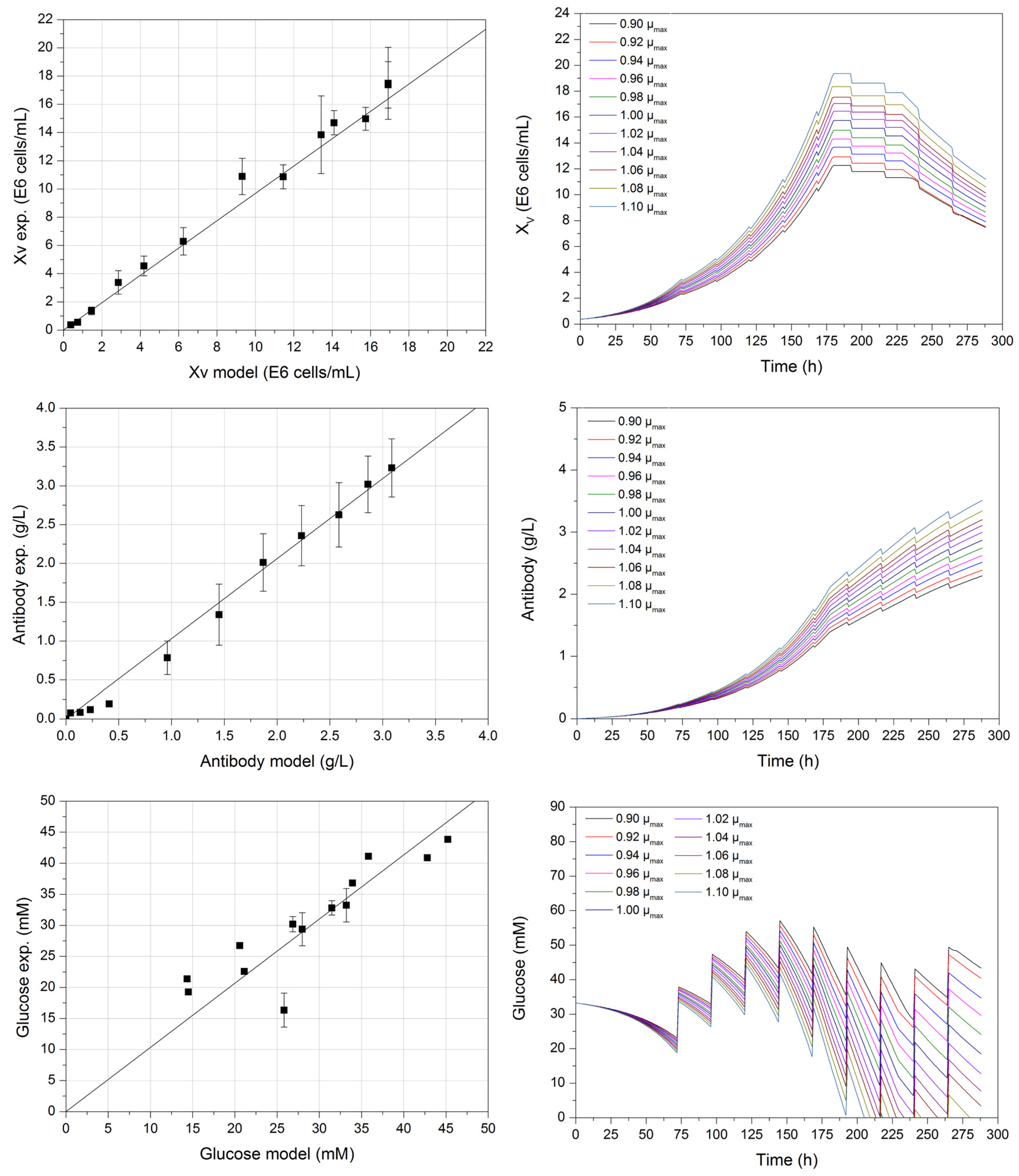
Figure 2 (left) depicts the verification of the computerized process model (first decision criterion), by comparing experimental data with model-derived results. The viable cell, product, and glucose concentration can be predicted sufficiently well. The coefficient of determination for each prediction is greater than 0.979, which is similar to the modelling of glucose concentration. Differences between the experimental and model-derived data are possible as a result of undescribed fluctuations under feed addition during cultivation in the kinetic model. These fluctuations mainly affect the glucose concentration, as other model variables such as lactate, antibody, or viable cells are not being fed. However, by adding feed, volumetric changes must be considered during the description of all variables.

Sensitivity studies such as the variation of one-parameter-at-a-time or design of experiments (DoE) are essential for detecting gross model errors. One-parameter-at-a-time variation of the maximum growth rate (±10% µ_max) can be seen in Figure 2 (right).

The higher µ_max, the steeper the exponential phase between 72 and 180 h of the viable cell concentration. This is mainly the result of a higher growth rate, which can be achieved during this phase, as can be seen in Equations (1) and (2). Therefore, the maximum growth rate has an impact on growth and maximum viable cell concentration in this macroscopic model, especially during the exponential phase. Corresponding to this increase in viable cell concentration, a higher product concentration can be observed, as well as a higher glucose consumption at the constant feed strategy, which is dependent on the current viable cell concentration at respective phases, as seen in Equation (4).

During one-parameter-at-a-time studies, the maximum growth rate exhibited the most significant influence on the course of the considered model variables. Therefore, a precise determination of this process model parameter is crucial for the precise modelling of dynamic cultivation processes, as the viable cell concentration X_V, and thus the growth rate µ, are present in the equations regarding substrates (4) and (6), metabolites (5) and (8), as well as product (9). This study indicates how important it is to accurately determine the model parameter to construct an accurate process model.

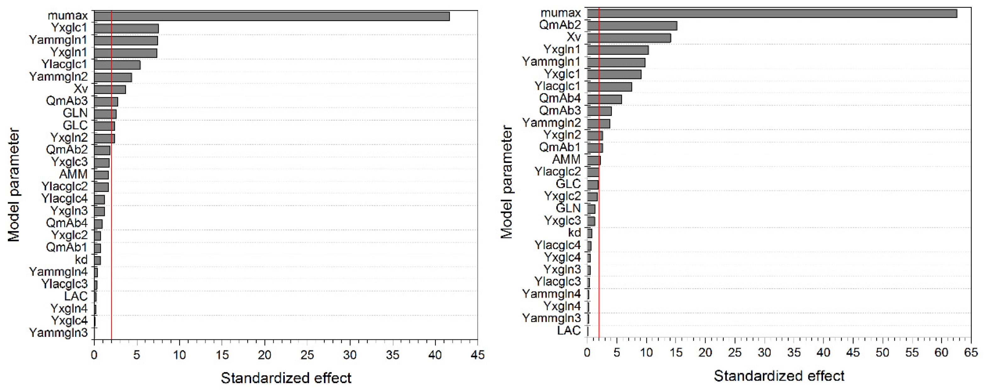
Simulations conducted by DoE approaches enable the quantitative determination of significant parameters. In addition, the variation of multiple parameters at the same time facilitates the coverage of parameter interactions during process modelling. For this, a fractional factorial design (resolution IV) consisting of all model parameters was conducted, resulting in 128 additional simulations.

The Pareto diagrams (Figure 3) indicate significant model parameters, based on a level of significance (α) set to 0.05 (second decision criterion). Besides the maximum growth rate µ_max, the yield coefficient Y_X/glc has a significant impact on the considered process variable (i.e., maximum viable cell concentration). Y_X/glc describes the ratio between generated viable cells (E6 cells/mL) and consumed glucose (mM). The higher Y_X/glc, the more cells can be generated during substrate uptake, as depicted in Equations (4) and (6). This results in a higher maximum viable cell concentration. The same correlation can be found considering Y_X/gln.

The yield coefficient Y_lac/glc, resembling the ratio between produced lactate (mM) and consumed glucose (mM), is shown to be a significant parameter by the pareto diagram in Figure 3 (left). As seen in Equations (2) and (5), a higher Y_lac/glc results in higher lactate concentrations and, therefore, in stronger inhibition of the growth rate and ultimately in a reduced maximum viable cell concentration. The same correlation can be found regarding Y_amm/gln.

Although the initial viable cell concentration possesses a significant influence on the maximum viable cell concentration, higher initial values result in an increase in substrate consumption and metabolite production, reducing the growth rate more rapidly, and may decrease the overall maximum viable cell concentration. The maximum death rate k_d possesses no significant effect on the maximum viable cell concentrations, as this parameter is strongly dependent on the current lactate and ammonium concentration. The higher the metabolite concentration, the higher the death rate µ_d, thus commonly resulting in a lower maximum viable cell concentration, as seen in Figure 2. However, these metabolites accumulate during cultivation and possess an impact only at the end of the process, after the maximum viable cell concentration has already been reached. Nevertheless, k_d exhibit a significant influence on the considered process variable because the apparent growth rate (µ minus µ_d) will be affected by the maximum death rate as well.

Similarities can be found regarding the pareto diagram in Figure 3 (right) for the maximum antibody concentration (mAb_max). In addition to the aforementioned correlations, the cell specific antibody production rate Q_mAb significantly influences the process variable mAb_max. However, the process parameter µ_max seems to be the most significant parameter for mAb_max, as well as for X_v,max, as can be seen in Figure 3 and in previous one-parameter-at-a-time studies in Figure 2.

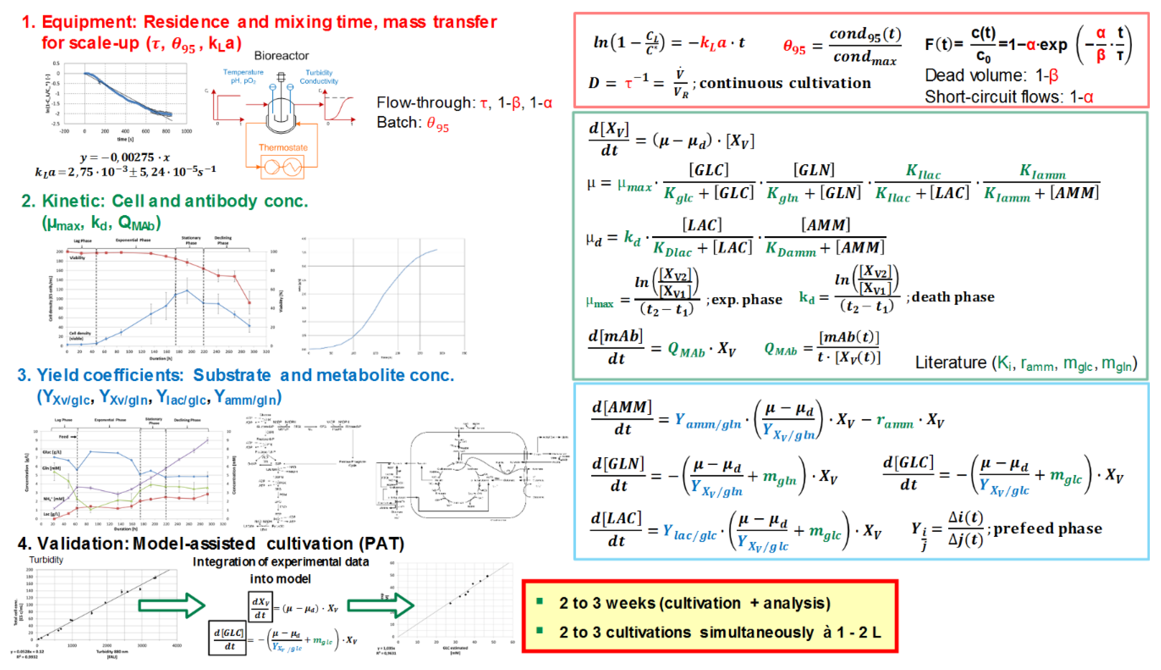
Model parameters are being quantitatively determined via experimental studies. The determination based on experimental data is afflicted with errors, for example, resulting from handling, repetitions, and measurement inaccuracies. Therefore, a model parameter determination concept must be implemented to evaluate the precision of the model (third decision criterion). The modelling approach for fed-batch and perfusion cultivation processes is summarized in Figure 4.

The main equations are represented by a Monod-type kinetic, considering the time-dependent variation of substrate (e.g., glucose, glutamine), metabolite (e.g., lactate, ammonium), cell, and product concentration. The correlation between input (e.g., substrate concentration) and output (e.g., cell concentration) variables can be macroscopically determined using empirical observations, such as yield coefficients, which are strongly dependent on the cell line and growth phase [14].

In terms of fluid dynamics (red-marked parameters), determination of oxygen transfer rates according to the unsteady-state (dynamic) technique, mixing times with conductivity measurements, and residence times with tracer experiments result in a characterization of the equipment.

Cultivations as well as the analysis of substrate, metabolite, cell, and product concentration need to be performed to determine kinetic (green-marked, for example, maximum growth rate) and equilibrium (blue-marked, for example, yield coefficients) parameters. The substrate saturation constants (or substrate affinity constants) equal concentrations that support a half-maximum growth rate.

Analog experiments can be used for validation. Furthermore, cultivations assisted by an online process model increase the gain in process information by integrating process data (e.g., turbidity) into the macroscopic kinetic model to extract information on process variables (e.g., glucose and lactate concentration) [11]. Efforts for the generation of this data are commonly 2 to 3 weeks for two to three simultaneously run cultivations in 1 to 2 L and their respective analysis.

The impact of experimental model parameter determination error on the process model, based on error propagation of experimental errors, must be assessed to evaluate model precision. These errors depict maximal and minimal values for each model parameter. This variance can be included into a Monte Carlo simulation to determine the effect of model parameter errors on the process model. In this case, 100 simulations, varying each parameter equally distributed based on their experimental errors, were conducted. An example of the distribution of model parameters is given in Figure 5. As can be seen, the equally distributed process parameters result in maximum and minimum values for each considered parameter. The arithmetic mean of each parameter is depicted as a red horizontal line and corresponds to the model parameter value in Table 2 (e.g., 0.029 h⁻¹ µ_max). This analysis shows the influence of model parameter errors and their interactions among each other on the macroscopic kinetic model.

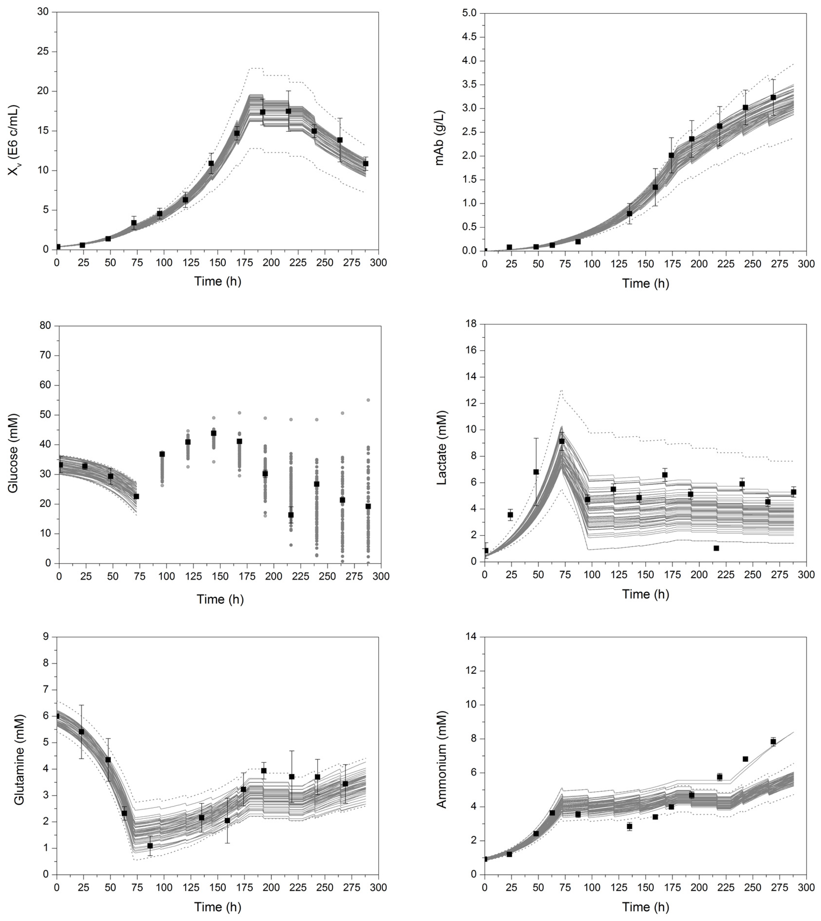
The Monte Carlo simulations resulted in a range of minimal and maximal values of each process variable, yielding enveloped curves, represented by grey lines (standard deviation of simulation results) in Figure 6. In addition to enveloped curves, represented by grey lines, the model is able to describe variations of process parameters, which occur with a lower probability (simulation result larger/smaller than standard deviation of mean simulation results), as depicted by the dotted lines. As can be seen, the variation of model parameters based on respective parameter errors leads to a variation in each process value. Maximum viable cell concentrations result in a higher substrate uptake and consumption, leading to a faster glucose and glutamine depletion. In addition, lactate, ammonium, and monoclonal antibody concentrations increase with higher viable cell concentrations. This analysis clearly shows the aforementioned precise model parameter determination. Especially, µ_max seems to be the key model parameter in this macroscopic kinetic model, as variations (±10% in Figure 2, as well as Monte Carlo based variations in Figure 6) result in a significant influence on the process model, as already shown by the DoE-based pareto diagrams in Figure 3. Sensor techniques such as turbidity (limited to cellular viability) and Raman spectroscopy (limited to a precise chemometric model) measuring the viable cell concentration online during mammalian cell cultivation support a precise determination of µ_max and, therefore, increase the precision of the process model (third decision criterion).

Partial least squares (PLS) regressions can be conducted to statistically evaluate the correlation between predictors (i.e., process parameters such as µ_max) and responses (i.e., process variables such as X_V,max). For this, the NIPALS (nonlinear iterative partial least squares) algorithm was used for the computation of factors. The data basis for this analysis is the results from the 100 Monte Carlo simulations. Each varied parameter set resulted in a specific outcome of process variables (e.g., maximum viable cell concentration, X_V), as seen in

Table 3. Example of the parameter set (X_V min) and target variable (X_V max) resulting from 100 Monte Carlo simulations.

Parameter Set	1	2	3	4	5	6	7	8	9	.....
XV min (E6 cells/mL)	0.37	0.32	0.42	0.36	0.38	0.40	0.34	0.32	0.37	.....
XV max (E6 cells/mL)	17.01	10.60	24.17	20.13	19.74	15.06	19.50	19.84	19.28	.....

.

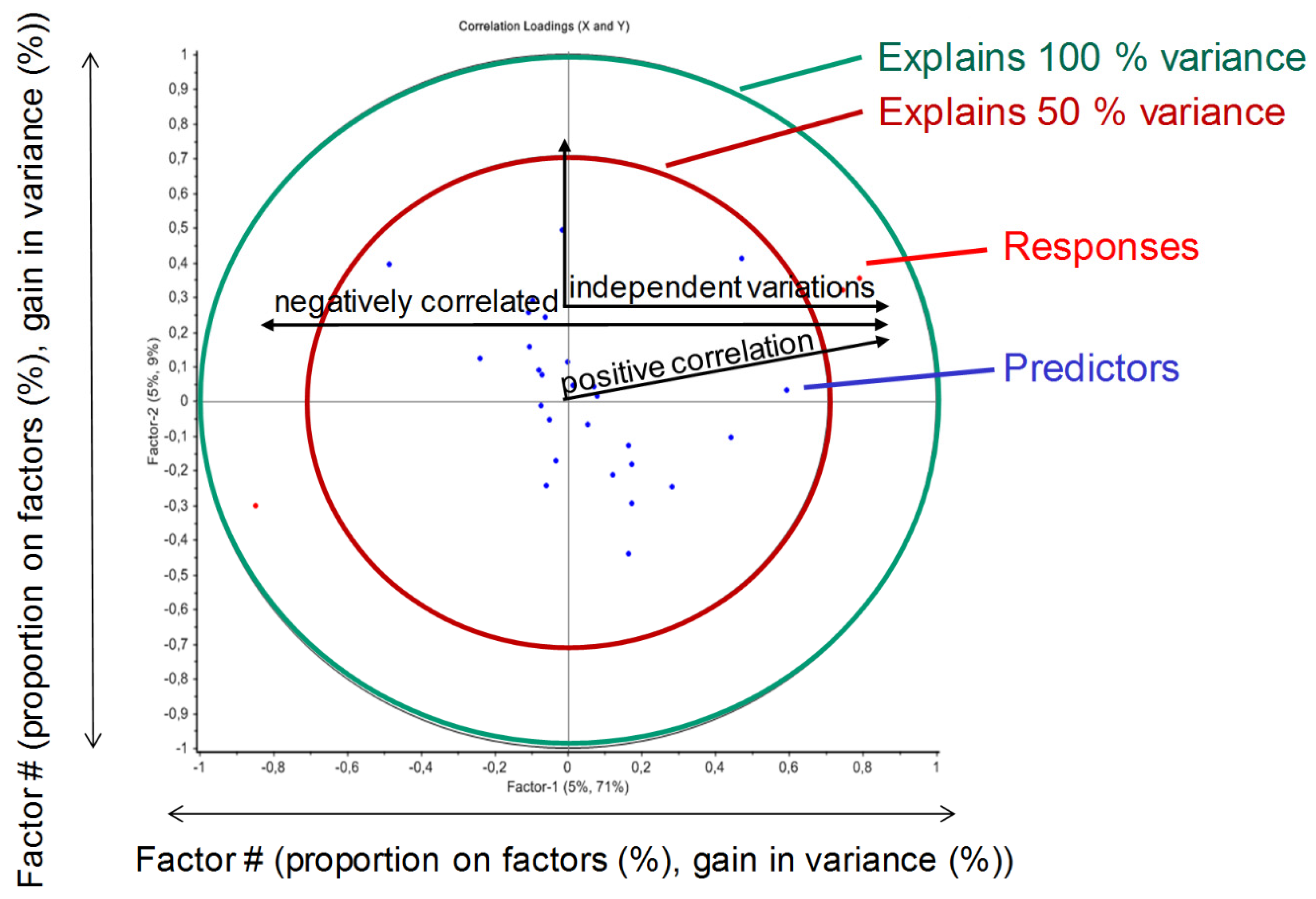
Figure 7 schematically describes the analysis of the correlation loadings based on the PLS regression. If responses and predictors are positive correlated to a specific factor (e.g., factor 1 or principal component 1, PC1), they are in relation to each other. In other words, a variation of the predictor possibly leads to a positive variation of the response. Opposite responses and predictors are negatively correlated, and 90° relationships do not induce a correlation (independent variation permitted), as they are correlated with different principal components. Higher orders of principal components would possibly be able to describe more variance, but are more affected by noise (i.e., PLS model is too detailed). Together, Table 3 and Figure 7 show the general principle of the implementation of PLS models to statistically evaluate Monte Carlo simulation results, as seen in Figure 8.

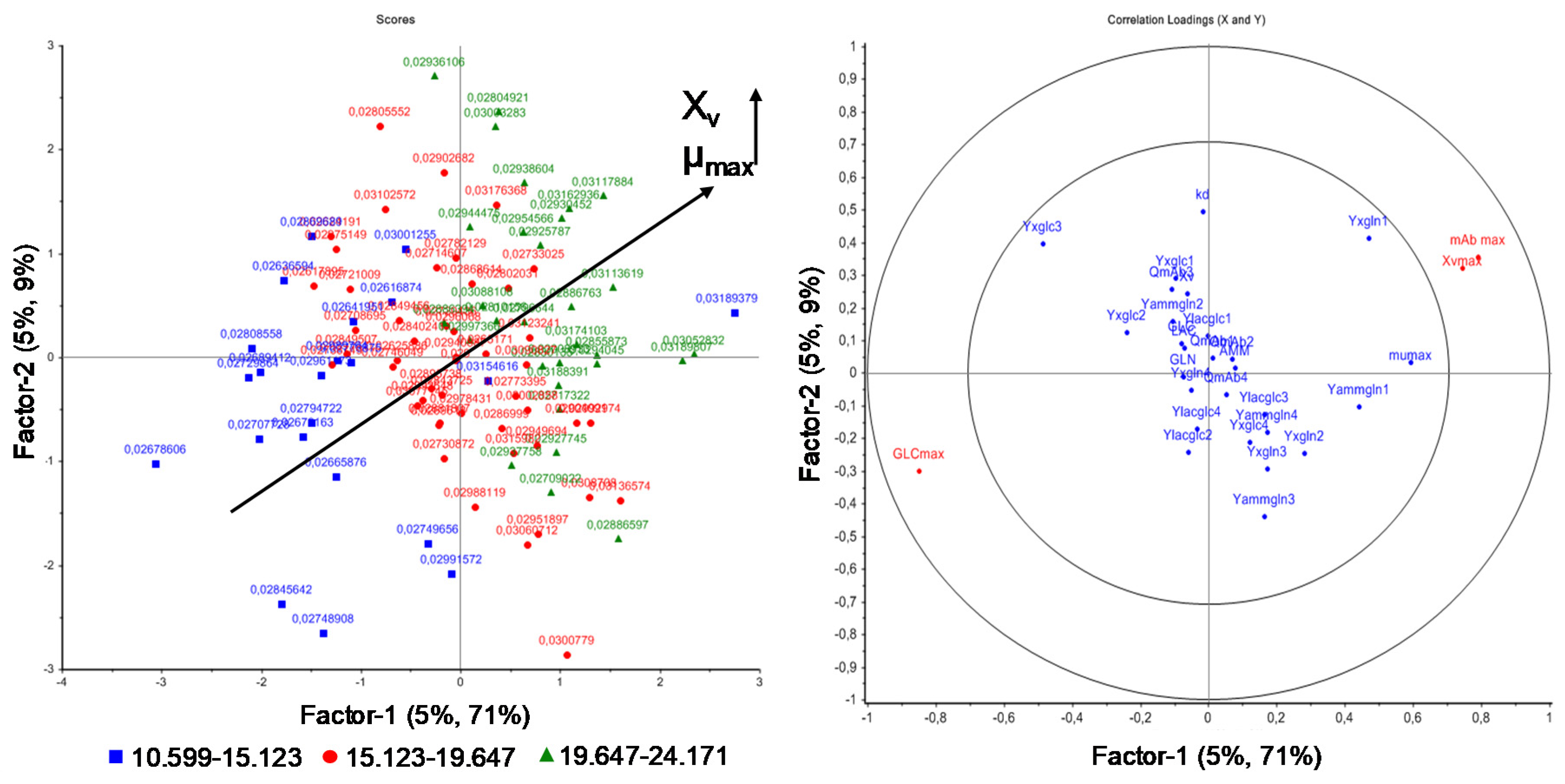
Figure 8 depicts the PLS regression of the influence of model parameter variation on the maximum viable cell, glucose, and antibody concentration. As can be seen, the maximum growth rate µ_max is strongly positive correlated with the maximum viable cell concentration X_V,max and negatively correlated with GLC_max (maximum glucose concentration). As already shown by one-parameter-at-a-time and DoE studies (Figure 2 and Figure 3), the higher µ_max, the higher X_V,max.

Additionally, Figure 8 depicts the influence of model parameter variation on the process variable GLC_max (maximum glucose concentration). The maximum growth rate µ_max is negatively correlated with GLC_max, as a higher growth rate results in an increased substrate uptake and consumption, as already seen in Figure 2.

The positive correlation of µ_max on the maximum viable cell concentration (X_V max) based on PLS analysis is shown in the score plot (Figure 8 left). The score plot identifies patterns in the samples, for example, by grouping responses and labeling predictors. The higher µ_max, the higher the maximum viable cell concentration, yielding higher antibody concentrations, as seen in Figure 2 and Equations (1) and (9). Interestingly, the cell specific antibody production rate Q_mAb can be independently varied. This may be the result of low variations of this process model parameter.

Concluding, as can be seen during one-parameter-at-a-time, DoE, and PLS studies, the maximum growth rate µ_max may be the key parameter of this macroscopic kinetic model based on Monod equations. A variation of µ_max exhibits a significant impact on growth, substrate consumption, and metabolite and product formation. This is mainly because of the dependency of each process variable on the viable cell concentration X_V, as seen in Equations (4) to (9). This dependency can also be seen during experimental cultivations. The strong dependency on cellular growth rate is, however, not surprising, but clearly shows the importance of a valid model parameter determination concept. The experimental determination of the maximum growth rate µ_max can be conducted by offline samples or, more preferably, by in situ probes such as turbidity or Raman spectroscopy [11], where data density, gain in information, and thus model accuracy and precision are increased.

4. Conclusions

The presented general valid model validation workflow is based on four criteria (verification, accuracy, precision, equality). On the basis of a literature review, a macroscopic model for the simulation of mammalian cell culture could be developed. The macroscopic model consists of Monod kinetic approaches for the simulation of time-dependent variations of substrate, metabolite, cellular, and product variables. A coefficient of determination of at least 0.97 (glucose concentration) could be achieved (verification). The accuracy was addressed by one-parameter-at-a-time and design of experiments studies in order to develop a Pareto plot to statistically determine significant parameters (accuracy). Therefore, a valid model parameter determination concept was generated to determine the effect of parameter determination error on the process model based on Monte Carlo simulations by equally distributing parameter determination errors (precision). PLS regressions were conducted to statistically evaluate the correlations between model parameters and variables, as well as correlations among model parameters themselves. PAT approaches to demonstrate the usability of this kinetic model were already applied (equality) [11]. Concluding, following the model validation workflow, process model understanding was increased by identifying key parameters (Figure 3), the impact of experimental parameter determination (Figure 6), as well as the correlation of model parameters between themselves and model variables (Figure 8).

References

- Hinz, D.C. Process analytical technologies in the pharmaceutical industry: The FDA’s PAT initiative. Anal. Bioanal. Chem. 2006, 384, 1036–1042. [Google Scholar] [CrossRef]
- Kornecki, M.; Schmidt, A.; Strube, J. Pat as Key-Enabling Technology for Qbd in Pharmaceutical Manufacturing—A Conceptual Review on Upstream and Downstream Processing. Chem. Today 2018, 36, 44–48. [Google Scholar]
- Krull, I.S.; Rakesh, M.; Anurag, S.R. Tools for Enabling Process Analytical Technology Applications in Biotechnology. BioPharm. Int. 2012. Available online: http://www.biopharminternational.com/tools-enabling-process-analytical-technology-applications-biotechnology-0?id=&pageID=1&sk=&date= (accessed on 20 March 2019).
- Sommerfeld, S.; Strube, J. Challenges in biotechnology production—Generic processes and process optimization for monoclonal antibodies. Chem. Eng. Process. Process Intensif. 2005, 44, 1123–1137. [Google Scholar] [CrossRef]
- Bechmann, J.; Rudolph, F.; Gebert, L.; Schaub, J.; Greulich, B.; Dieterle, M.; Bradl, H. Process parameters impacting product quality. BMC Proc. 2015, 9, O7. [Google Scholar] [CrossRef]
- FDA. Guidance for Industry. PAT—A Framework for Innovative Pharmaceutical Development, Manufacturing, and Quality Assurance. Available online: https://www.fda.gov/downloads/drugs/guidances/ucm070305.pdf (accessed on 19 February 2018).
- FDA; CDER; CBER; USDHHS. Pharmaceutical Development Q8(R2). 2009. Available online: https://www.ich.org/fileadmin/Public_Web_Site/ICH_Products/Guidelines/Quality/Q8_R1/Step4/Q8_R2_Guideline.pdf (accessed on 19 February 2018).
- Oyeleye, O.; Ogundeji, S.T.; Ola, S.I.; Omitogun, O.G. Basics of animal cell culture: Foundation for modern science. BMBR 2016, 11, 6–16. [Google Scholar] [CrossRef]
- Präve, P. (Ed.) Handbook of Biotechnology, 4th ed.; Oldenbourg: Munich, Germany, 1994. [Google Scholar]
- Musmann, C.; Joeris, K.; Markert, S.; Solle, D.; Scheper, T. Spectroscopic methods and their applicability for high-throughput characterization of mammalian cell cultures in automated cell culture systems. Eng. Life Sci. 2016, 16, 405–416. [Google Scholar] [CrossRef]
- Kornecki, M.; Strube, J. Process Analytical Technology for Advanced Process Control in Biologics Manufacturing with the Aid of Macroscopic Kinetic Modeling. Bioengineering 2018, 5, 25. [Google Scholar] [CrossRef] [PubMed]
- Uhlenbrock, L.; Sixt, M.; Strube, J. Quality-by-Design (QbD) process evaluation for phytopharmaceuticals on the example of 10-deacetylbaccatin III from yew. Resour. Eff. Technol. 2017, 3, 137–143. [Google Scholar] [CrossRef]
- Zobel-Roos, S.; Schmidt, A.; Mestmäcker, F.; Mouellef, M.; Huter, M.; Uhlenbrock, L.; Kornecki, M.; Lohmann, L.; Ditz, R.; Strube, J. Accelerating Biologics Manufacturing by Modelling OR: Is approval under the QbD- and PAT-approach demanded by authorities still appropriate without a digital-twin? Processes 2019, 7, 94. [Google Scholar] [CrossRef]
- Ben Yahia, B.; Malphettes, L.; Heinzle, E. Macroscopic modeling of mammalian cell growth and metabolism. Appl. Microbiol. Biotechnol. 2015, 99, 7009–7024. [Google Scholar] [CrossRef]
- Goudar, C.T. Computer programs for modeling mammalian cell batch and fed-batch cultures using logistic equations. Cytotechnology 2012, 64, 465–475. [Google Scholar] [CrossRef] [PubMed]
- Goudar, C.T.; Joeris, K.; Konstantinov, K.B.; Piret, J.M. Logistic equations effectively model mammalian cell batch and fed-batch kinetics by logically constraining the fit. Biotechnol. Prog. 2005, 21, 1109–1118. [Google Scholar] [CrossRef]
- Goudar, C.T.; Konstantinov, K.B.; Piret, J.M. Robust parameter estimation during logistic modeling of batch and fed-batch culture kinetics. Biotechnol. Prog. 2009, 25, 801–806. [Google Scholar] [CrossRef] [PubMed]
- Jang, J.D.; Barford, J.P. An unstructured kinetic model of macromolecular metabolism in batch and fed-batch cultures of hybridoma cells producing monoclonal antibody. Biochem. Eng. J. 2000, 4, 153–168. [Google Scholar] [CrossRef]
- Sidoli, F.R.; Mantalaris, A.; Asprey, S.P. Modelling of Mammalian Cells and Cell Culture Processes. Cytotechnology 2004, 44, 27–46. [Google Scholar] [CrossRef]
- Hefzi, H.; Ang, K.S.; Hanscho, M.; Bordbar, A.; Ruckerbauer, D.; Lakshmanan, M.; Orellana, C.A.; Baycin-Hizal, D.; Huang, Y.; Ley, D.; et al. A Consensus Genome-scale Reconstruction of Chinese Hamster Ovary Cell Metabolism. Cell Syst. 2016, 3, 434–443. [Google Scholar] [CrossRef] [PubMed]
- Selişteanu, D.; Șendrescu, D.; Georgeanu, V.; Roman, M. Mammalian Cell Culture Process for Monoclonal Antibody Production: Nonlinear Modelling and Parameter Estimation. BioMed Res. Int. 2015, 2015. [Google Scholar] [CrossRef]
- Chen, N.; Bennett, M.H.; Kontoravdi, C. Analysis of Chinese hamster ovary cell metabolism through a combined computational and experimental approach. Cytotechnology 2014, 66, 945–966. [Google Scholar] [CrossRef] [PubMed]
- Nicolae, A.; Wahrheit, J.; Bahnemann, J.; Zeng, A.-P.; Heinzle, E. Non-stationary 13C metabolic flux analysis of Chinese hamster ovary cells in batch culture using extracellular labeling highlights metabolic reversibility and compartmentation. BMC Syst. Biol. 2014, 8, 50. [Google Scholar] [CrossRef]
- Wahrheit, J.; Nicolae, A.; Heinzle, E. Dynamics of growth and metabolism controlled by glutamine availability in Chinese hamster ovary cells. Appl. Microbiol. Biotechnol. 2014, 98, 1771–1783. [Google Scholar] [CrossRef] [PubMed]
- Borchers, S.; Freund, S.; Rath, A.; Streif, S.; Reichl, U.; Findeisen, R. Identification of growth phases and influencing factors in cultivations with AGE1.HN cells using set-based methods. PLoS ONE 2013, 8, e68124. [Google Scholar] [CrossRef] [PubMed]
- Ahn, W.S.; Antoniewicz, M.R. Parallel labeling experiments with 1,2-(13)Cglucose and U-(13)Cglutamine provide new insights into CHO cell metabolism. Metab. Eng. 2013, 15, 34–47. [Google Scholar] [CrossRef]
- Ghorbaniaghdam, A.; Henry, O.; Jolicoeur, M. A kinetic-metabolic model based on cell energetic state: Study of CHO cell behavior under Na-butyrate stimulation. Bioprocess Biosyst. Eng. 2013, 36, 469–487. [Google Scholar] [CrossRef] [PubMed]
- Martinez, V.S.; Dietmair, S.; Quek, L.-E.; Hodson, M.P.; Gray, P.; Nielsen, L.K. Flux balance analysis of CHO cells before and after a metabolic switch from lactate production to consumption. Biotechnol. Bioeng. 2013, 110, 660–666. [Google Scholar] [CrossRef] [PubMed]
- Templeton, N.; Dean, J.; Reddy, P.; Young, J.D. Peak antibody production is associated with increased oxidative metabolism in an industrially relevant fed-batch CHO cell culture. Biotechnol. Bioeng. 2013, 110, 2013–2024. [Google Scholar] [CrossRef] [PubMed]
- Zamorano, F.; Vande Wouwer, A.; Jungers, R.M.; Bastin, G. Dynamic metabolic models of CHO cell cultures through minimal sets of elementary flux modes. J. Biotechnol. 2013, 164, 409–422. [Google Scholar] [CrossRef] [PubMed]
- Ahn, W.S.; Antoniewicz, M.R. Metabolic flux analysis of CHO cells at growth and non-growth phases using isotopic tracers and mass spectrometry. Metab. Eng. 2011, 13, 598–609. [Google Scholar] [CrossRef] [PubMed]
- Naderi, S.; Meshram, M.; Wei, C.; McConkey, B.; Ingalls, B.; Budman, H.; Scharer, J. Development of a mathematical model for evaluating the dynamics of normal and apoptotic Chinese hamster ovary cells. Biotechnol. Prog. 2011, 27, 1197–1205. [Google Scholar] [CrossRef]
- Nolan, R.P.; Lee, K. Dynamic model of CHO cell metabolism. Metab. Eng. 2011, 13, 108–124. [Google Scholar] [CrossRef]
- Xing, Z.; Bishop, N.; Leister, K.; Li, Z.J. Modeling kinetics of a large-scale fed-batch CHO cell culture by markov chain monte carlo method. Biotechnol. Prog. 2010, 26, 208–219. [Google Scholar] [CrossRef] [PubMed]
- Xing, Z.; Li, Z.; Chow, V.; Lee, S.S. Identifying inhibitory threshold values of repressing metabolites in CHO cell culture using multivariate analysis methods. Biotechnol. Prog. 2008, 24, 675–683. [Google Scholar] [CrossRef]
- Gao, J.; Gorenflo, V.M.; Scharer, J.M.; Budman, H.M. Dynamic metabolic modeling for a MAB bioprocess. Biotechnol. Prog. 2007, 23, 168–181. [Google Scholar] [CrossRef]
- Kontoravdi, C.; Asprey, S.P.; Pistikopoulos, E.N.; Mantalaris, A. Development of a dynamic model of monoclonal antibody production and glycosylation for product quality monitoring. Comput. Chem. Eng. 2007, 31, 392–400. [Google Scholar] [CrossRef]
- Teixeira, A.P.; Alves, C.; Alves, P.M.; Carrondo, M.J.T.; Oliveira, R. Hybrid elementary flux analysis/nonparametric modeling: Application for bioprocess control. BMC Bioinform. 2007, 8, 30. [Google Scholar] [CrossRef]
- Provost, A.; Bastin, G.; Agathos, S.N.; Schneider, Y.J. Metabolic design of macroscopic bioreaction models: Application to Chinese hamster ovary cells. Bioprocess Biosyst. Eng. 2006, 29, 349–366. [Google Scholar] [CrossRef]
- Oliveira, R. Combining first principles modelling and artificial neural networks: A general framework. Comput. Chem. Eng. 2004, 28, 755–766. [Google Scholar] [CrossRef]
- Vande Wouwer, A.; Renotte, C.; Bogaerts, P. Biological reaction modeling using radial basis function networks. Comput. Chem. Eng. 2004, 28, 2157–2164. [Google Scholar] [CrossRef]
- Sainz, J.; Pizarro, F.; Perez-Correa, J.R.; Agosin, E. Modeling of yeast metabolism and process dynamics in batch fermentation. Biotechnol. Bioeng. 2003, 81, 818–828. [Google Scholar] [CrossRef]
- Altamirano, C.; Illanes, A.; Casablancas, A.; Gamez, X.; Cairo, J.J.; Godia, C. Analysis of CHO cells metabolic redistribution in a glutamate-based defined medium in continuous culture. Biotechnol. Progress 2001, 17, 1032–1041. [Google Scholar] [CrossRef]
- Nyberg, G.B.; Balcarcel, R.R.; Follstad, B.D.; Stephanopoulos, G.; Wang, D.I.C. Metabolism of peptide amino acids by Chinese hamster ovary cells grown in a complex medium. Biotechnol. Bioeng. 1999, 62, 324–335. [Google Scholar] [CrossRef]
- Kornecki, M.; Mestmäcker, F.; Zobel-Roos, S.; Heikaus de Figueiredo, L.; Schlüter, H.; Strube, J. Host Cell Proteins in Biologics Manufacturing: The Good, the Bad, and the Ugly. Antibodies 2017, 6, 13. [Google Scholar] [CrossRef]
- Subramanian, G. (Ed.) Continuous Biomanufacturing//Continuous Biomanufacturing. Innovative Technologies and Methods; Wiley-VCH: Weinheim, Germany, 2017. [Google Scholar]
Figure 1.
General valid model validation workflow [13]. Macroscopic kinetic models simulating the dynamic state of a cell culture can gather essential information about cellular conditions (e.g., lag, exponential, stationary, decline phase), substrate uptake, metabolite, and productivity, as well as possible feeding adjustments [14,15,16,17,18,19]. A combination of online turbidity data resembling the cell concentration and a macroscopic kinetic model was already applied to estimate substrate and metabolite concentrations [11]. A general overview of several working groups focusing on upstream process modelling is presented in Table 1. DoE, design of experiments; MC, Monte Carlo.
Figure 2.
Correlation (left) between experimental and model-derived viable cell (R2 ≥ 0.98), glucose (R2 ≥ 0.97), and antibody concentration (R2 ≥ 0.99) with a maximum growth rate of 0.029 h−1. One-parameter-at-a-time studies (right) of the macroscopic model exemplified by varying the maximum growth rate ±10% of the experimental determined value.
Figure 3.
Pareto diagram of standardized effects for the determination of significant model parameters on the response of maximum viable cell concentration XV,max (left) and maximum antibody concentration mAbmax (right). The vertical red line depicts the reference line for statistical significance, which is 1.98 for both model variables. The level of significance α was 0.05 for both model variables. Numbers indicate model parameter used in respective phase: 1, lag; 2, exponential; 3, stationary; 4, decline.
Figure 4.
Schematic workflow overview for the model parameter determination concept in upstream process modelling. Detailed description can be found in the literature [2,11,13,14,45,46]. Red-marked parameters (volumetric mass transfer coefficient kLa, mixing time θ95, as well as residence time) lead to the characterization of the equipment. Kinetic (green-marked) and equilibrium (blue-marked) parameters can be obtained by cultivations. For validation, similar experiments can be used. Efforts for the generation of this data are commonly 2 to 3 weeks for two to three simultaneously run cultivations in 1 to 2 L and their respective analysis. GLC, glucose, GLN, glutamine; LAC, lactate; AMM, ammonium, PAT, process analytical technology.
Figure 5.
Example of the distribution of model parameters, resulting from 100 Monte Carlo simulations, varying each parameter equally distributed based on their experimental error. The horizontal line depicts the arithmetic mean of each parameter.
Figure 6.
Enveloped curves of each process variable resulting from 100 model parameter error-based Monte Carlo simulations. Xv, viable cell concentration; mAb, monoclonal antibody. Black square dots represent experimental data. Error bars comprise the standard deviation of three cultivations. For better clarity and visualization, the enveloping curves for glucose after 72 h show the starting concentrations before respective feed addition. The detailed course of glucose between feed additions can be seen in Figure 2.
Figure 7.
Schematic presentation of a loadings plot resulting from a partial least squares (PLS) regression.
Figure 8.
PLS regression loadings (right) for the maximum viable cell concentration XV,max, maximum glucose concentration (GLCmax), and maximum antibody concentration (mAbmax) as response, depending on model parameters (predictors) as well as PLS regression scores (left) grouped into the correlation between maximum growth rate µmax and XV.