Modeling of Parallel Movement for Deep-Lane Unit Load Autonomous Shuttle and Stacker Crane Warehousing Systems

1
School of Control Science and Engineering, Shandong University, Jinan 250061, Shandong, China
2
School of Mechanical Engineering, Shandong University, Jinan 250061, Shandong, China
3
School of Software, Shandong University, Jinan 250061, Shandong, China
*
Authors to whom correspondence should be addressed.
Processes 2020, 8(1), 80; https://0-doi-org.brum.beds.ac.uk/10.3390/pr8010080
Submission received: 7 November 2019
/
Revised: 29 December 2019
/
Accepted: 4 January 2020
/
Published: 7 January 2020
(This article belongs to the Special Issue Synergies in Combined Development of Processes and Models)
Abstract
:The autonomous shuttle and stacker crane (AC/SC) warehousing system, as a new automated deep-lane unit load storage/retrieval system, has been becoming more popular, especially for batch order fulfilment because of its high flexibility, low operational cost and improved storage capacity. This system consists of a shuttle sub-system that controls motion along the x-axis and a stacker crane sub-system that controls motion along the y-axis and z-axis. The combination of shuttles and a stacker crane performs storage and retrieval tasks. Modelling the parallel motion is an important design tool that can be used to calculate the optimal number of shuttles for a given configuration of the warehousing system. In this study, shuttle movements from one lane to another are inserted into the stock-keeping unit (SKU) task queue, and convert such that they are consistent with the retrieval tasks. The tasks are then grouped according to their starting lane, and converted to an assembly-line parallel job problem by analysing the operating mode with the objectives of minimising the total working time of the stacker crane and the wasted shuttle time. A time sequence mathematical model based on the motion of the shuttles and stacker crane is proposed, and an improved Pareto-optimal elitist non-dominated sorting genetic algorithm is used to solve this multi-objective optimization problem. The model is validated via a simulation study, and via a real-world warehousing case study. We go on to describe guidelines for the layout and configuration of AS/SC warehousing systems, including the optimal number of shuttles and number of x-axis storage cells of lanes, which can improve efficiency and minimise both capital investment and operating costs.
1. Introduction
The autonomous shuttles and stacker crane (AS/SC) warehousing system is a recently introduced automated warehousing technique for storage and retrieval tasks. Compared with a conventional automated storage and retrieval system (AS/RS), it exhibits superior space utilization because of the presence of multiple unit-load storage locations in each lane (in the depth direction). With conventional AS/RS, each storage or retrieval task is fulfilled using an aisle-captive stacker crane that exhibits horizontal and vertical movement, and which may retrieve at most two load units in the depth direction. By contrast, with an AS/SC warehousing system, the shuttles can move unit loads in the depth direction, and the stacker crane moves the unit loads directly. Thus, AS/SC is more flexible and is characterized by low operating costs.
Such deep-lane unit load storage systems are characterized by high space-usage efficiency, and are suitable for storing products with relatively low variation but large quantity in unit-load demand [1,2]. The AS/SC warehousing system is a compact storage system, and has recently attracted much attention of logistics companies. The AS/SC warehousing system has become increasingly popular, and researches on its applications can be found in many studies [3,4]. It’s very widely used in some production industries, including refrigerated warehousing, where it is shown to reduce the required refrigerated space and hence the cooling costs, as well as in distribution centers connected to production lines, and distribution centers where the flexible bulk storage system could feed into the forward pick areas [5,6,7]. Some examples include drinks production systems for mineral water and soft drink products. With these systems, as with a generic production line, batches of unit load with the same SKU are created, and the batch production planning and material handling system supplies the end-of-line unit-load warehouses. Because the quantity is high, AS/SC can provide high storage density and reduce the transport time via shuttles working simultaneously in different lanes. To maximize throughput, when unit loads are outbound, the tasks for a given item should continue as far as possible, and the first outbound in the lane should be that with the nearest aisle of tasks.
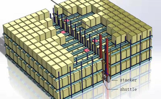
As shown in Figure 1, this new application inherits the merits of the AS/RS, and improves space utilization and storage capacity, as well as flexibility. AS/SC warehousing systems represent an improvement of AS/RS in terms of batch production and order processing, whereby shuttles can move between lanes via the stacker crane [8,9]. AS/SC warehousing systems have a stacker crane in each aisle and several shuttles. Motion in the y-axis and z-axis is enabled by the stacker crane. The shuttles move back and forth along the x-axis and deliver unit loads to the first storage cell of each lane. The unit loads are stored along the lane according to a last-in-first-out (LIFO) policy. The shuttle stops in the default dwell unit of the last previously inserted palletized lane, and performs the next retrieving or stocking action applied to that batch SKU. If a shuttle is required to switch to another lane, it must first move to the first storage unit of the current lane. Although each shuttle can execute all storage and retrieval tasks, the inbound shuttle and outbound shuttle will be located in different aisles if the storage and retrieval tasks are executed at the same time. In general, the number of shuttles in each aisle is determined by the number of different SKUs for simultaneous storage or retrieval tasks. For example, if there are two production lines that produce different SKUs, or there are two outbound loading stations, at least two shuttles would usually be required, one for each SKU. However, in some scenarios, there may be too few shuttles to cope with variations in demand. Moreover, the size of the warehouse can significantly affect the system efficiency. Determining the required number of shuttles based on scheduling of tasks in order to minimize the total operating time is not straightforward, but is a problem that should be resolved as part of the design of an AS/SC system.
AS/SC warehousing systems can only implement a LIFO policy in each x-axis lane for storage and retrieval activities, and the lane containing unit loads stores the same SKU and production batch. Different batches are dynamically assigned to different lanes. A new batch may require several empty lanes that had previously been assigned to other items or batches. The required number of empty lanes therefore depends on the size of the incoming batch.
AS/SC warehousing systems are similar to the drive-in racks and flown-rack systems, so the adoption of AS/SC may significantly increase the storage area utilization. The aim and the main contributions of this paper are as follows:
- The time operating model based on AS/SC system is established physical structure and scheduling methods.
- A method to solve AS/SC system shuttle vehicle configuration by optimizing time model was proposed.
- Simulation results show the effectiveness of the model.
This paper is organized as follows: Section 2 provides a review of AS/SC warehousing systems. Section 3 analyses the expected operational cycle length when retrieving a unit load. Section 4 describes the multi-objective optimization model. Section 5 proposes a detailed solution to group scheduling problem using a variant of the GA, and we validate the model and algorithm using a practical engineering example in Section 6. Section 7 presents the conclusions and some insights for future study.
2. Literature Review
Many reports have been published in the field of compact storage systems; however, they typically focus on shuttle-based compact storage systems, which use lifts rather than a stacker crane. These kinds of papers can be divided into those on conveyor and stacker crane compact storage systems and those on autonomous vehicle storage and retrieval systems (AVS/RS). Park and Webster were the first to describe a compact storage system [10,11]. They proposed a conceptual framework for warehouse planning and design of a compact storage system considering control procedures, vertical and horizontal movement, and storage rack structure. They also described a storage structure layout method called cubic-in-time, which minimizes the travel time of selected handling equipment in a three-dimensional palletized storage system. De Koster et al. investigated the optimal storage rack of a conveyor mechanism, and reported an approximate travel time expression for dual command cycles, which was used to optimize the system dimensions [2]. Malmborg was the first scholar to evaluate the AVS/RS and propose analytical tools based on the features of autonomous vehicle systems to model the expected performance as functions of key system attributes, including the storage capacity, rack configuration and fleet size [12]. He extended with the number of pending transactions in the state space description. However, the state equation method is less efficient in solving large-scale problems [13]. In addition, EKren reported a simulation regression analysis of the rack configuration of an AVS/RS, and described mathematical functions for the rack configuration that reflected the relationship between the outputs (responses) and the input variables (factors) of the system under various scenarios [14]. Furthermore, Zaerpour proposed a mathematical model for a shared storage policy that minimized the total retrieval time [15].
A number of papers have reported analytical models using a queueing network approach to describe the system performance of AVS/RS [16]. Fukunari reported a model of a lift service process as an M/G/L queue nested within an M/G/V queue, modelling the vehicle service considering both single- and dual-command cycles [17]. In addition, Kuo used a semi-open queueing network to model an AVS/RS, solving the network using a matrix-geometric method [18]. Heragu modelled variations of AVS/RS using an open queueing network, and analyzed performance using the manufacturing system performance analyzer (MPA). Experimental results shown that the MPA may be a better choice than simulation studies to evaluate alternative configurations quickly [19]. Recently, Roy et al. reported a model of a single-time AVS/RS using a multi-class semi-open queueing network with class switching, and developed a decomposition-based approach to evaluate system performance. Their results suggest that the best system performance can be found when the depth-to-width ratio is 2 for an AVS/RS system with the middle lift [20]. In another study, Roy et al. modeled the system as an integrated queuing network and estimated the cycle time and resource utilization of the system [21]. They modeled each layer as a semi-open queuing network and the vertical transfer unit as a multi-class queuing network, with each vertical transfer segment corresponding to G/G/1 queue. They addressed the integration model by capturing the connections between arrival and departure points in the tier subsystem and the vertical transfer unit. Marchet et al. optimize the shape of the system by simulating an AVS/RS system with a tier-captive configuration [22]. In their results, the impact of rack configuration on throughput performance was illustrated. Manzini used a simulation approach to investigate analytical models for different layout configurations, distinguishing the location of input/output points and the so-called shape ratio [23]. To validate these models, researchers adopted simulation that includes cycle time and distance and turned out to be a useful tool to evaluate the performance of warehousing systems and can provide practical guidance for storage system design. In another study, Wang discussed multi-tier shuttle warehousing systems, and created a retrieval task model that was solved by Pareto optimization using an elitist non-dominated sorting GA [8]. Their results show the optimization solution can reduce the total idle time of lift and shuttle. Furthermore, Tappia developed novel queueing network models to describe the performance of single-tier and multi-tier shuttle-based compact systems [7]. Finally, Zou proposed a parallel policy for tier-captive AVS/RSs, and formulated a fork-join queueing network to analyze system performance [16].
As for travel time model, Lerher et al. developed travel time models for single-deep AVS/RS and double-deep AVS/RS respectively. They proposed a closed expression of cycle time and consider the effects of shuttle acceleration and deceleration [24,25]. Fukunari and Malmborg developed an efficient cycle time model, but they also considered single or double deep racks, not deep-lane unit-load systems [26]. Manzini et al. developed an efficient analytical model for the travel time and distance in single and dual-command cycles and give a layout configuration [23]. D’Antonio et al. proposed an analytical model which is used to calculate the cycle time and evaluate its deviation [27]. Guerrazzi et al. developed a simulator able to emulate the operation of the warehouse, considering travel-time and energy model [28]. The number of research articles on AS/SC warehouse systems is limited. Because the operating strategy of AVS/RS is similar to that of an AS/SC warehousing system, some of the corresponding methods can be applied. Most studies have focused on conceptual analytical methods. To improve the efficiency of the warehousing system, it is essential to consider the optimal configuration of the devices to operate simultaneously. In this work, we model the AS/SC warehousing system to optimize the configuration, and optimize task scheduling to increase efficiency.
3. System Description
AS/SC warehousing systems have a unique structure, as shown in Figure 1. Shuttles perform storage and retrieval tasks in each lane (x-axis). A stacker crane is located at the center of each aisle, and controls vertical (z-axis) and horizontal motion (y-axis). All storage and retrieval tasks are completed using both a shuttle and a stacker crane. Although this combination requires more time for a single task than conventional AS/RS, the parallel performance of multi-tier shuttles can result in significant improvements in operational efficiency and space utilization.
To analyze the system performance and model the parallel motion of shuttles and the stacker crane, we make a number of assumptions that have been widely used in previous papers, and also take practical operating characteristics into account. The assumptions are illustrated as follows:
- (1)
- Simple operating mode. Storage and retrieval customer orders are fulfilled in different time windows. We consider only retrieval tasks as an example in the analysis.
- (2)
- Transaction requests vehicle based on first-come-first-serve (FCFS). Both shuttles and the stacker crane conform to this principle. Each order shares the same priority level.
- (3)
- All tasks are grouped according to the outbound lane.
- (4)
- The rack is considered to be continuous and rectangular, and the stacker crane can reach any location in the aisle. This assumption makes problem analysis much easier, and the results are usually close enough to the real world [29].
- (5)
- The length of the rack is significantly greater than the height. This is one widely used principle in warehouse design.
- (6)
- Dwell point policy. The stacker crane remains where it is after completing a storage and retrieval operation. Shuttles return to the handover station of current lane upon finishing a job.
- (7)
- Random storage. Any location is equally likely for storage or retrieval of a unit load [30].
- (8)
- The loading and unloading times at the destination position for a given load or shuttle are known and constant. Each unit load has a standard pallet, and requires a fixed time for loading or unloading.
- (9)
- The job sequence is continuous and there is no prior information for a specific retrieval task [31].
- (10)
- Each lane has the same depth on both sides of the main cross aisle.
- (11)
- The acceleration and deceleration of the stacker crane in the horizontal and vertical directions are constant and equal. Each task will undergo an acceleration and a deceleration period. Each storage or retrieval operation therefore has a specific kinematics model, which includes acceleration, deceleration and the maximum velocity restrictions.
- (12)
- The shuttle in charge of orthogonal depth motion is assumed to move at a constant velocity.
- (13)
- The inventory is sufficient for retrieval SKUs.
Retrieval tasks are critical to system performance, and here we consider retrieval tasks with the abovementioned assumptions. In addition to a few tasks whose starting position is the first unit storage location in the lane, the shuttles and stacker crane jointly complete most of the retrieval tasks, as shown in Figure 2. When the warehouse control system (WCS) assigns a retrieval task to the relevant lane and there is an available shuttle in that lane, if it is idle, the shuttle approaches the retrieval position of the task. The shuttle loads the pallet and carries it to the first storage cell of the lane where the shuttle can transfer the pallet to the stacker crane, and then returns to the default dwell point to await handover. If there are no shuttles in the retrieval task lane, the WCS sends the nearest idle shuttle to the first storage cell. As soon as the shuttle responsible for carrying the pallet moves to the dwell point or arrives at the first storage cell for preparation to move to the next task lane, it sends a stacker crane delivery request (SCDR) to the monitoring system. All SCDR tasks are executed based on the FCFS principle. Once the stacker crane arrives at the dwell point in the corresponding lane, the pallet or shuttle is transferred to the stacker crane. If the stacker crane is carrying a pallet, the WCS releases the shuttle for the subsequent retrieval task in the corresponding lane. The stacker crane continues to the destination position, carrying the pallet or shuttle. Finally, the stacker crane is released when the pallet or shuttle is unloaded at the destination position. When a shuttle carried by a stacker crane is unloaded, that shuttle should approach the dwell position for the new retrieval task.
When a series of retrieval tasks arrive at the AS/SC warehousing system, some may be executed in parallel by multi-lane shuttles. Each required pallet or shuttle is then transferred to the destination by the stacker crane in sequence. The operation of an AS/SC warehousing system can be characterized as parallel retrieval and sequential transfer (PRST). This PRST-based operation differs significantly from the traveling salesman problem model, which is commonly used to model AS/RS [32].
4. System Modeling
In the previous section, Figure 2 shows the PRST operating process of an AS/SC warehousing system. Every retrieval transaction of shuttles or stacker crane depends on the finishing time of the previous movement, the location of the storage position, and the dwell point policy. Firstly, some basic notations are shown as follows:
| The number of shuttles | The time to traverse the width of a storage cell | ||
| Q | The number of tasks | The time for the shuttle to load or unload a unit load | |
| D | The width of the storage rack | H | The height of the storage rack |
| N | The number of different lanes for all tasks | The time for the stacker crane to pick up or release the pallet or a shuttle | |
| The number of storage cells in the x-axis (lane depth) | The dwell point of a shuttle in a lane | ||
| p | The length of a single storage cell in the x-axis | The x-axis starting position of task i | |
| The width of a single storage cell in the y-axis | The y-axis starting position of task i | ||
| The height of a single storage cell in the z-axis | The z-axis starting position of task i | ||
| The acceleration/deceleration of the stacker crane in the y-axis | The x-axis end position of task i | ||
| The acceleration/deceleration of the stacker crane in the z-axis | The y-axis end position of task i | ||
| The maximum velocity of the stacker crane in the y-axis | The z-axis end position of task i | ||
| The maximum velocity of the stacker crane in the z-axis |
First, we define the array variable , which describes the relation between the task group and retrieval task in each lane [33]. The value of is a unique task ID assigned to the group , and when the number of tasks in this group is less than , . The last element of each group is reserved for transferring shuttle tasks. Any members of the group has the following constraints:
S.t
where is the number of all tasks described by . In the same group one task’s start position could be less than next task’s, and the number of tasks must be less than .
When the tasks in group are finished and there are tasks in other lane waiting to be executed, motion to transfer a shuttle is necessary. The number of shuttle transfer tasks depends on the number of lanes and the number of shuttles . The sum of all tasks , including the outbound task and shuttle transfer tasks, is derived as follows:
When the shuttle is to transfer from one lane to another lane, it approaches to the first storage position where the stacker crane can pick it. The stacker crane loads the shuttle and carries it to the destination lane. The shuttle then moves to the dwell point of the new lane. The process includes horizontal movement of the shuttle, stacker crane movement, and the shuttle returning to the default dwell point . The process of transferring a shuttle is therefore equivalent to the process of retrieving a unit load, and the starting position in the coordinate system of this type of transfer task for the stacker crane is as follows:
where are the y-axis and z-axis position of the present task for the stacker crane respectively.
Generally, the end location of transferring tasks is depending on the next group where there is no available shuttle in the lane:
where are the y-axis and z-axis position of the transferring task for the shuttle respectively. And is the new group dwell point for the shuttle.
Shuttle transfer tasks are inserted into the task group and placed at the end of group , and may be considered as an outbound task. We consider all task queues covering the outbound and shuttle transfer tasks.
To obtain the total time for an operation, we analyze the times for individual task, as shown in Figure 3.
Here is the time for finished task , and sequential superscripts are used to represent critical timing throughout the cycle period; respectively, represents the time when the shuttle begins a retrieval task, is the time when the shuttle places a unit load into the first storage cell and sends an SCDR until it returns to the dwell point, corresponds to the time when the stacker crane begins to respond to the SCDR of task , and indicates the time when the unit load or shuttle has been transferred to the stacker crane.
Several shuttles may execute tasks simultaneously; however, their finishing times may be different. According to the FCFS principle, there may be two types of stagnation period during the task execution period, as shown in Figure 4. These stagnation periods are critical for operational efficiency, as well as overall system performance. The first type of stagnation period is stacker crane idle time (SCIT), which is denoted , and occurs when an SCDR has not been made after the stacker crane finished the previous task. The second type of stagnation period is shuttle wasting time (SWT), and is induced when a shuttle sends an SCDR while the stacker crane is fulfilling a previous task, and is indicated by .
Thus, the following two situations may occur during each retrieval task period.
In general, all shuttles operate in parallel, and most tasks will be characterized by , where except where two simultaneous tasks originate from the same lane and there is no other task currently being executed.
If SCIT occurs, there is no SWT; then, , .
If SWT occurs, there is no SCIT; then, , .
In the two both cases, is defined for the first type of stagnation period is stacker crane idle time (SCIT), and is defined for the second type of stagnation period is shuttle wasting time (SWT).
The variables and represent the probabilities of SCIT and SWT, respectively, and are defined as follows:
Thus, the accumulative and of SCIT and SWT for all tasks can be determined using Equations (2), (5) and (6):
where is defined for the total stacker crane working time (SCWT) for retrieval task .
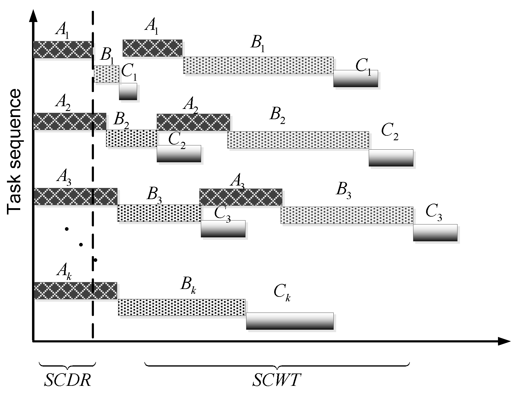
While the shuttle executes task or , the stacker crane may implement task or task . Although shuttles can execute different tasks in parallel, and the shuttle operating time may differ, SCIT and SWT occur frequently in a single retrieval task and the horizontal movement of unit loads in the lane may be implemented by a different shuttle. Eventually, all tasks should be fulfilled by the stacker crane, including shuttle transfer from one lane to another. Therefore, the total SCWT can be regarded as the main control time line, and used to calculate the total outbound time (TOT). As shown in Figure 5, warehousing operations can be divided into three stages, based on the stacker crane operating process.
- Stage A: The shuttle retrieves a unit load. The shuttle travels forward to retrieve the required unit load from the default dwell point to the storage position, carries it to the first storage cell of the lane, returns to the default dwell point and sends an SCDR to the stacker crane. If the unit load is stored in the first location of the lane, this time for this stage is zero. If the task is shuttle transfer, the shuttle should approach the first storage cell and send an SCDR.
- Stage B: The shuttle transfers the unit load to the stacker crane. The stacker crane responds to the SCDR, travels to the retrieval lane, and then completes transfer to the required unit load or shuttle. The AS/SC warehousing system releases the shuttle at the end of this stage. SCIT is included in this stage.
- Stage C: Operation of the stacker crane. The stacker crane travels to the destination position and unloads the required SKU or shuttle. The AS/SC warehousing system releases the stacker crane at the end of this stage.
The entire warehousing operation process can be regarded as an assembly line production mode; i.e., the TOT is the sum of the time of the first SCDR and the total SCWT.
The time for the shuttle to execute retrieval task in the first stage, represented by , is as follows:
When the SKU is located at the start of the lane (i.e., ), the task time for the shuttle is zero.
The time required by the stacker crane for stages B and C is then as follows:
where is the SCIT for task , whose minimum value is zero; is the time for the stacker crane to travel from its current position to the lane for a particular task ; and is the time for the stacker crane to travel from the lane for task to the destination position. The time is influenced by the acceleration and deceleration of the stacker crane, and can be calculated based on one of four cases.
First, the velocity of the stacker crane may not reach its maximum in either direction (i.e., the velocity components and in the horizontal and vertical directions, respectively):
S.t
S.t
where in Equation (11) which is founded according to velocity formula, the stacker crane is accelerating and may not the maximum in both y and z directions. is the distance traveled by acceleration. Equation (12) has the same meaning as Equation (11). and can be found in Equation (10).
Second, the horizontal velocity of the stacker crane can reach the maximum speed , but this cannot be achieved in the vertical direction:
S.t
S.t
In this case, reaches its maximum and not. is the time for the stacker crane to accelerate to the maximum speed in the y-axis direction. is the time for the stacker to travel to the target position at a constant maximum speed in the direction of y-axis. represents the driving distance of the stacker must be greater than the maximum acceleration distance. Equation (14) has the same meaning as Equation (13).
Third, the stacker crane does not reach in the horizontal direction, but does reach in the vertical direction:
S.t
S.t
This case is the opposite of the second, reaches its maximum and not.
The final scenario is that the stacker crane can reach the max velocity both in horizontal direction and vertical direction:
S.t
S.t
In this case, and reaches its maximum respectively.
From Equations (1), (4) and (7), the total SCWT can be obtained iteratively as follows:
where the variable can be found in Equation (7) and Equations (11)–(18).
We calculate the total TOT as the sum of the operating times for the stacking crane and the first SCDR time:
where is the time for the shuttle to execute retrieval task in Equation (9).
We calculate the total TOT as the sum of the operating times for the stacking crane and the first SCDR time. The sequence of tasks can affect the total time, so the task scheduling problem of the automated warehousing system in part involves adjusting and re-scheduling the task execution sequence in a given time window under given constraints in order to minimize the total time for the tasks. The above discussion suggests that the two stagnation points can influence the performance of an AS/SC warehousing system. A longer SCIT will reduce the stacker crane utilization rate, increasing TOT. A longer SWT will not influence the TOT, instead generating a queue of retrieval tasks waiting in storage lanes, which negatively influences the shuttle utilization rate and results in a waste of equipment time. Therefore, the objective model for an AS/SC warehousing system should consider the shortest TOT, SCIT and SWT for a series of retrieval tasks, as well as shuttle transfer tasks, within a given time window. The objective used is as follows:
S.t
In the objective function (21), which is equal to the Equation (19), represents to minimize the TOT, the sum of the time of the first SCDR and the total SCWT. Equation (2) minimizes the shuttle wasting time. The variables can be found using Equations (11)–(18). Condition is the maximum idle time of the stacker crane, and is the maximum waste time for each shuttle. and can be set in advance, depending on the specific requirements. Constraints represents the initial position. The terms are used to record the current position of shuttle .
5. Model Solution
The task sequencing problem of 2D system with the DC mode is proved to be NP-hard [34]. Even though we only focus on retrieval tasks in a 3D AS/SC with the SC mode, the problems will not become easier because of the following reasons: (1) The units in a 3D system is greater than in a 2D system. (2) In this system, we have to transfer shuttles across lanes. (3) The problem can be much more difficult if there are different types of SKUs in one lane.
The operating mode of an AS/SC warehousing system is similar to that of a flexible multi-machine scheduling problem based on makespan. It is an NP-complete problem, which is a classic problem in the field of workshop manufacturing systems, and has been studied extensively. In recent years, genetic algorithms have been widely used to solve these problems. A large number of studies have proposed methods of solving parallel multi-machine problems using simple GAs, adaptive GAs, parallel GAs, hybrid GAs and GAs based on the combination rule. When the results of the objective functions are more than one, the problem is transformed into a multi-objective optimization problem. Solving the scheduling model essentially involves all permutations and combinations of tasks; however, in practice, there may be a large number of tasks within a single window time, and hence it may not be feasible to explore all task sequences. To solve this multi-objective optimization problem (MOOP), we use the operating characteristics of the AS/SC warehousing system and the improved elitist non-dominated sorting GA (NSGA-II) to minimize the total outbound operating time. Since it was first proposed by Deb [35], the NSGA-II algorithm has been widely used to solve MOOP problems [23,32]. The algorithm is also widely used in multi-objective optimization of automatic warehouse model [8,36,37]. In a multi-criteria decision-making theory, pareto optimality decision rationality is the necessary condition. So, the problem of MOOP “reasonable” solutions should be pareto optimality, while NSGA-II is a method used to solve the problem of MOOP, so the optimal solution of NSGA-II for any problem should be pareto optimality. In this problem, any solution of the pareto optimal front forms an optimal solution with tradeoff between two objectives. It is left to the decision maker for choice of the solution among the pareto optimal solutions. The key steps in the solution process are as follows.
5.1. Encodings
Based on the grouping characteristics and the definition of , we use a natural number coding system for the candidate solutions of practical engineering problems to describe the execution sequence of group tasks in the same lane. Once the group sequence is determined, the tasks can be executed in order, which, if not zero-valued, can be described by an array of columns such as , , . Because the scale N of the chromosome is determined by the number of groups, the chromosome is indicated by , where represents the determined working sequence of the group task. In group , one possibility of the sequences of group task could be or .
5.2. Fitness Function
The fitness function is based on the TOT and SWT, and used to evaluate the adaptability of the chromosome in the entire population. Generally speaking, the optimization goal is the maximum value, which is more acceptable and understandable. To evaluate the solution, the minimized objectives should be transferred to a maximization problem as follows:
where , are the maximum values we set and , are their transformed fitness values.
5.3. Non-Dominated Sort
The critical factor of the MOOP is how to determine the Pareto optimal solution set of the objective function. In each generation, the population is sorted based on non-dominated Pareto optimality. First, the initial-tier Pareto set is determined based on the multi-objective function value. We then remove the initial Pareto set from the population. The subsequent Pareto front set in the remaining population is then found from the non-dominated set as the second-tier Pareto set . The process is repeated until all individuals (chromosomes) are sorted. The individuals in the identical-tier Pareto set have equal virtual fitness. Individuals in the small-tier rank are selected as high-priority elitists.
5.4. Crowding Distance
Once non-dominated sorting is completed, the crowding distance for individuals in each Pareto front set is calculated. This is indicated by the rectangle that covers individual , but no others. The calculation of the crowding distance in the improved elitist non-dominated sorting GA is an important step that ensures the diversity of the population, and proceeds as follows:
- (a)
- The crowding distance is set to zero.
- (b)
- For each objective, the population is sorted and the crowding distance between pairs of border individual chromosomes is set to infinity.
- (c)
- This distance is recalculated as the accumulated sum of the fitness values of the two chromosomes and :where M is the number of optimization goals, and are the fitness values of the optimization goal m for chromosomes and , and and are the maximum and minimum fitness values, respectively.
- (d)
- During population maintenance, each individual is removed and the crowding distance between the remaining individuals in the population is recalculated based on the concept of the dynamic crowding distance introduced by Yu. et al. [38]. The variance of the clustering distance from each individual i is used to indicate the difference in crowding distances for each objective, so that individuals with larger differences have greater chance to remain:We then convert to , which is the dynamic crowding distance:
5.5. Elitism Strategy
Screening of parents and offspring is carried out according to an elite strategy. In generation t, the virtual fitness value and crowding distance matrix for tiers of individuals are merged with a parent set , yielding an offspring set , which depends on the virtual fitness value and crowding distance of population G. Then, fills in population until the size of population n reaches the number of setting N.
5.6. Selection, and Genetic Operators
The genetic operator is similar to that of a simple GA. The offspring set is reproduced for the individual set that removes the retained elite strategy individuals via a tournament selection operator, a single-point crossover operator and a tentative gene mutation operator. The parent elite set and offspring set compose the population of the next generation .
5.7. Termination Condition
With NSGA-II, the termination criterion is typically a fixed number of generations (maximum iteration).
6. Case Study and Model Validation
To verify the objective model, we chose the data from the logistics distribution center of a pharmaceutical enterprise. This distribution center contains an automated warehousing system with several autonomous shuttles, one stacker crane and a matched conveyor system. The warehouse management system (WMS) automatically gathers all the required customer orders in a single time window, with reference to this AS/SC warehousing system, and then generates retrieval tasks. Subsequently, the warehouse control system (WCS) groups the tasks according to their starting lane, and then reshuffles task groups using our scheduling model. The WCS dispatches jobs to relevant shuttles ordered by the shuttle numbers and x-axis locations. Each unit load is transferred to the I/O station via shuttle and the stacker crane. The equipment operating parameters are as bellows: , , , , , and . Other system configurations are .
The number of storage cells in the x-axis is k, where k > 7 and k can be regarded as a variable. To simulate this scenario, we assume that the x-axis position of each task varies with the number of storage cells. For example, if the number of storage cells is 7, then = 5; however, when there are 8 storage cells, = 6. The number of storage cells in the y-axis is 74, and there are 6 storage cells in the z-axis.
The WMS gathers 60 retrieval unit load requests in a single time window, the number of lanes is N = 28, and the initial number of storage cells is k = 7. These requests are listed in Table 1.
The WCS determines the optimal execution sequence based on the objective model using NSGA-II. The initial population size is 28, based on the initial parameters, and the maximum number of generations is 3000. The crossover rate is 0.9 and the mutation rate 0.1.
After some simulation experiments, we obtained a set of Pareto optimal solutions and found the optimal number of shuttles with various unit depths. We obtained TOT and SWT with varying numbers of shuttles and depths, as shown in Figure 6 and Figure 7.
Where there are only 1 shuttle, according to Figure 6, the TOT is obviously far more than any other number of shuttles. The unit number of x direction influence TOT significantly. The reason is that it is easy to schedule a shuttle, but a shuttle does not move in parallel when it runs. And the stacker crane’s waiting time becomes longer distinctly, when k is large, the time became worse, thus reducing the efficiency of outbound. In this situation, SWT is short because this shuttle may be work longer than others.
When there are three or four shuttles, TOT and SWT are optimized. If there is only a single shuttle, the change of depth k influenced TOT significantly; however, when there are three or four shuttles, k had little effect. When there are more than four shuttles, TOT is acceptable but SWT increased rapidly. This is because there are too many shuttles, but only one stacker crane. The stacker crane has limited capacity and can only release or load a limited number of shuttles or pallet per operating cycle. Therefore, in a certain period of time, multiple shuttle vehicles will be idle. When we used a general stacker crane with fewer than 30 storage cells in the x-axis, the optimal number of shuttles for the warehousing system is 4.
The case shows that time model established by this design of the AS/SC system can solve the warehouse problem better, and NSGA-II is used to obtain the experimental results. Model can also be used to optimize the configuration of warehouse layout and shuttle task. Other researches of similar system time models, most of which assume that the number of shuttles is a constant, often study the optimal configuration of rack or layout [7,20,23]. Roy et al. builds a queuing model to accommodate a wide variety of design configurations that differ in terms of D/W ratio, vehicle assignment rules, and number of zones, but as the number of zones increases, system performance degrades due to increased transaction waiting time due to increased waiting time for vehicles. In this paper, the model constraints and objective functions are simple and it is easy to implement and apply.
7. Conclusions
This paper proposed a model for the operating time of an AS/SC warehousing system. By grouping tasks, the task scheduling problem is transformed into a set of group scheduling problems. The operation time for a single task is divided into the pickup time of the shuttle, the transfer times for the shuttle and the stacker crane, the total operating time for the stacker crane, and waiting times of shuttles and the stacker crane. Several shuttles are considered working in parallel with a single stacker crane, so the problem is converted into an assembly line production model according to the operating mode. Generally, the stacker crane is the bottleneck of an AC/SC warehousing system, so the total SCWT should be regarded as the main objective if we wish to minimize the total time. The model has two optimization objectives: the minimum TOT of the stacker crane, and the SWT for a given time window. The improved NSGA-II is used to solve this multi-objective group scheduling model and convert to group arrays as the basis of the task queue. A case study is carried out to verify the model and obtain optimized number of shuttles for various numbers of different storage cells in the x-axis.
In this study, we make several assumptions that may be studied in future research. For example, in this paper we consider only randomized storage strategy. Therefore, other storage policies (e.g., class-based or dedicated storage) can be considered as well. Meanwhile, our further research can also focus on a variable shuttle velocity or insufficient inventory in each lane. This topic provides an interesting direction for future research, and the improvement of the model and the enhancement of algorithms may be used to obtain precise results.
Author Contributions
Conceptualization, Y.W.; Data curation, R.M.; Formal analysis, X.Z.; Funding acquisition, Y.W.; Investigation, R.M.; Methodology, X.Z.; Project administration, H.L.; Resources, H.L.; Supervision, X.Z.; Validation, H.L.; Writing—original draft, Y.W.; Writing—review & editing, R.M. All authors have read and agreed to the published version of the manuscript.
Funding
This research was funded by the Fundamental Research Funds for Shandong University, grant number 2018JC035.
Conflicts of Interest
The authors declare no conflict of interests.
References
- Hu, Y.H.; Huang, S.Y.; Chen, C.; Hsu, W.J.; Toh, A.C.; Loh, C.K.; Song, T. Travel time analysis of a new automated storage and retrieval system. Comput. Oper. Res. 2005, 32, 1515–1544. [Google Scholar] [CrossRef]
- De Koster, R.; Le-Duc, T.; Yu, Y. Optimal storage rack design for a 3-dimensional compact AS/RS. Int. J. Prod. Res. 2008, 46, 1495–1514. [Google Scholar] [CrossRef] [Green Version]
- Gue, K.R. Very high-density storage systems. IISE Trans. 2006, 38, 79–90. [Google Scholar] [CrossRef]
- Yu, Y.; De Koster, M. Designing an optimal turnover-based storage rack for a 3D compact automated storage and retrieval system. Int. J. Prod. Res. 2009, 47, 1551–1571. [Google Scholar] [CrossRef]
- Westfalia. High Density, Multiple Deep AS/RS. Available online: https://www.westfaliausa.com/products/automated-storage-retrieval-systems/storage-density (accessed on 6 December 2019).
- Abelwomack. Deep Lane High Density Pallet Storage: Unique Storage Technology that Maximizes Warehouse Space. Available online: https://www.abelwomack.com/deep-lane-high-density-pallet-storage (accessed on 6 December 2019).
- Tappia, E.; Roy, D.; Koster, R.D.; Melacini, M. Modeling, analysis, and design insights for shuttle-based compact storage systems. Soc. Sci. Electron. Publ. 2017, 51, 269–295. [Google Scholar] [CrossRef] [Green Version]
- Wang, Y.; Mou, S.; Wu, Y. Task scheduling for multi-tier shuttle warehousing systems. Int. J. Prod. Res. 2015, 53, 5884–5895. [Google Scholar] [CrossRef]
- Wang, Y.; Mou, S.; Wu, Y. Storage assignment optimization in a multi-tier shuttle warehousing system. Chin. J. Mech. Eng. 2016, 29, 421–429. [Google Scholar] [CrossRef]
- Park, Y.H.; Webster, D.B. Modeling of three-dimensional warehouse systems. Int. J. Prod. Res. 1989, 27, 985–1003. [Google Scholar] [CrossRef]
- Park, Y.H.; Webster, D.B. Design of class-based storage racks for minimizing travel time in a three-dimensional storage system. Int. J. Prod. Res. 1989, 27, 1589–1601. [Google Scholar] [CrossRef]
- Malmborg, C.J. Conceptualizing tools for autonomous vehicle storage and retrieval systems. Int. J. Prod. Res. 2002, 40, 1807–1822. [Google Scholar] [CrossRef]
- Malmborg, C.J. Interleaving dynamics in autonomous vehicle storage and retrieval systems. Int. J. Prod. Res. 2003, 41, 1057–1069. [Google Scholar] [CrossRef]
- Ekren, B.Y.; Heragu, S.S. Simulation-based regression analysis for the rack configuration of an autonomous vehicle storage and retrieval system. Int. J. Prod. Res. 2010, 48, 6257–6274. [Google Scholar] [CrossRef]
- Zaerpour, N.; Yu, Y.G.; De Koster, R.B.M. Storing Fresh Produce for Fast Retrieval in an Automated Compact Cross-Dock System. Prod. Oper. Manag. 2015, 24, 1266–1284. [Google Scholar] [CrossRef] [Green Version]
- Zou, B.; Xu, X.; Gong, Y.M.; De Koster, R. Modeling parallel movement of lifts and vehicles in tier-captive vehicle-based warehousing systems. Eur. J. Oper. Res. 2016, 254, 51–67. [Google Scholar] [CrossRef] [Green Version]
- Fukunari, M.; Malmborg, C.J. A network queuing approach for evaluation of performance measures in autonomous vehicle storage and retrieval systems. Eur. J. Oper. Res. 2009, 193, 152–167. [Google Scholar] [CrossRef]
- Kuo, P.H.; Krishnamurthy, A.; Malmborg, C.J. Design models for unit load storage and retrieval systems using autonomous vehicle technology and resource conserving storage and dwell point policies. Appl. Math. Model. 2007, 31, 2332–2346. [Google Scholar] [CrossRef]
- Heragu, S.S.; Cai, X.; Krishnamurthy, A.; Malmborg, C. Analytical models for analysis of automated warehouse material handling systems. Int. J. Prod. Res. 2011, 49, 6833–6861. [Google Scholar] [CrossRef]
- Roy, D.; Krishnamurthy, A.; Heragu, S.S.; Malmborg, C. Performance analysis and design trade-offs in warehouses with autonomous vehicle technology. IIE Trans. 2012, 44, 1045–1060. [Google Scholar] [CrossRef]
- Roy, D.; Krishnamurthy, A.; Heragu, S.S.; Malmborg, C. A multi-tier linking approach to analyze performance of autonomous vehicle-based storage and retrieval systems. Comput. Oper. Res. 2017, 83, 173–188. [Google Scholar] [CrossRef] [Green Version]
- Marchet, G.; Melacini, M.; Perotti, S.; Tappia, E. Development of a framework for the design of autonomous vehicle storage and retrieval systems. Int. J. Prod. Res. 2013, 51, 4365–4387. [Google Scholar] [CrossRef]
- Manzini, R.; Accorsi, R.; Baruffaldi, G.; Cennerazzo, T.; Gamberi, M. Travel time models for deep-lane unit-load autonomous vehicle storage and retrieval system. Int. J. Prod. Res. 2016, 54, 4286–4304. [Google Scholar] [CrossRef]
- Lerher, T. Travel time model for double-deep shuttle-based storage and retrieval systems. Int. J. Prod. Res. 2016, 54, 2519–2540. [Google Scholar] [CrossRef]
- Lerher, T.; Ekren, B.Y.; Dukic, G.; Rosi, B. Travel time model for shuttle-based storage and retrieval systems. Int. J. Adv. Manuf. Technol. 2015, 78, 1705–1725. [Google Scholar] [CrossRef]
- Fukunari, M.; Malmborg, C. An efficient cycle time model for autonomous vehicle storage and retrieval systems. Int. J. Prod. Res. 2008, 46, 3167–3184. [Google Scholar] [CrossRef]
- D’Antonio, G.; Maddis, M.D.; Bedolla, J.S.; Chiabert, P.; Lombardi, F. Analytical models for the evaluation of deep-lane autonomous vehicle storage and retrieval system performance. Int. J. Adv. Manuf. Technol. 2018, 94, 1811–1824. [Google Scholar] [CrossRef]
- Guerrazzi, E.; Mininno, V.; Aloini, D.; Dulmin, R.; Scarpelli, C.; Sabatini, M. Energy Evaluation of Deep-Lane Autonomous Vehicle Storage and Retrieval System. Sustainability 2019, 11, 3817. [Google Scholar] [CrossRef] [Green Version]
- Hausman, W.H.; Schwarz, L.B.; Graves, S.C. Optimal storage assignment in automatic warehousing systems. Manag. Sci. 1976, 22, 629–638. [Google Scholar] [CrossRef]
- Warehouse Science. Warehouse and Distribution Science. Available online: http://www.warehouse-science.com (accessed on 6 December 2019).
- Bozer, Y.A.; White, J.A. Travel-time models for automated storage/retrieval systems. IIE Trans. 1984, 16, 329–338. [Google Scholar] [CrossRef]
- Wang, Y.; Zhou, Y.; Shen, C.; Wu, Y. Applicability Selection Method of Two Parts-to-picker Order Picking Systems. J. Mech. Eng. 2015, 51, 206–212. [Google Scholar] [CrossRef]
- Yi, Y.; Wang, D. Scheduling Grouped Jobs on Parallel Machines with Setups. Comput. Integr. Manuf. Syst. 2001, 7, 7–11. [Google Scholar]
- Han, M.H.; McGinnis, L.F.; Shieh, J.S.; White, J.A. On sequencing retrievals in an automated storage/retrieval system. IISE Trans. 1987, 19, 56–66. [Google Scholar] [CrossRef]
- Deb, K.; Pratap, A.; Agarwal, S. A fast and elitist multiobjective genetic algorithm: NSGA-II Evolutionary Computation. IEEE Trans. 2002, 6, 182–197. [Google Scholar]
- Diao, X.; Li, H.; Zeng, S.; Tam, V.W.; Guo, H. A Pareto multi-objective optimization approach for solving time-cost-quality tradeoff problems. Technol. Econ. Dev. Econ. 2011, 17, 22–41. [Google Scholar] [CrossRef]
- Rajković, M.; Zrnić, N.; Kosanić, N.; Borovinšek, M.; Lerher, T. A multi-objective optimization model for minimizing investment expenses, cycle times and CO2 footprint of an automated storage and retrieval systems. Transport 2019, 34, 275–286. [Google Scholar] [CrossRef] [Green Version]
- Yu, T.F.; Wang, B.; Peng, C.H. Improved non-dominated sorting genetical algorithm applied in multi-objective optimization of coal fired boiler combustion. Appl. Res. Comput. 2013, 301, 180–182. [Google Scholar]
Figure 1.
Layout of an AC/SC warehousing system.


Figure 2.
Flow diagram for retrieval tasks in an AS/SC warehousing system.

Figure 3.
Cycle time analysis for the task.

Figure 4.
Analysis of the stagnation period.

Figure 5.
Analysis of working time of shuttles and stacker crane.

Figure 6.
Total TOT.

Figure 7.
Total SWT.


Table 1.
All retrieval tasks and their original retrieval positions.
| Sequence | X | Y | Z | Task Number |
|---|---|---|---|---|
| 1 | 5 | 3 | 1 | 2 |
| 2 | 5 | 4 | 2 | 1 |
| 3 | 4 | 4 | 3 | 2 |
| 4 | 3 | 5 | 4 | 1 |
| 5 | 2 | 6 | 5 | 4 |
| 6 | 3 | 7 | 1 | 3 |
| 7 | 3 | 10 | 5 | 3 |
| 8 | 4 | 10 | 1 | 2 |
| 9 | 3 | 11 | 2 | 2 |
| 10 | 3 | 13 | 3 | 2 |
| 11 | 3 | 14 | 4 | 1 |
| 12 | 5 | 15 | 5 | 1 |
| 13 | 4 | 20 | 2 | 2 |
| 14 | 4 | 22 | 3 | 3 |
| 15 | 4 | 24 | 5 | 1 |
| 16 | 3 | 24 | 1 | 3 |
| 17 | 4 | 30 | 5 | 1 |
| 18 | 4 | 31 | 1 | 3 |
| 19 | 3 | 32 | 2 | 2 |
| 20 | 3 | 34 | 3 | 4 |
| 21 | 3 | 35 | 4 | 4 |
| 22 | 5 | 37 | 5 | 2 |
| 23 | 1 | 43 | 2 | 1 |
| 24 | 5 | 44 | 3 | 2 |
| 25 | 4 | 47 | 4 | 1 |
| 26 | 6 | 51 | 1 | 1 |
| 27 | 4 | 54 | 2 | 2 |
| 28 | 2 | 55 | 3 | 4 |
© 2020 by the authors. Licensee MDPI, Basel, Switzerland. This article is an open access article distributed under the terms and conditions of the Creative Commons Attribution (CC BY) license (http://creativecommons.org/licenses/by/4.0/).
Share and Cite
MDPI and ACS Style
Wang, Y.; Man, R.; Zhao, X.; Liu, H. Modeling of Parallel Movement for Deep-Lane Unit Load Autonomous Shuttle and Stacker Crane Warehousing Systems. Processes 2020, 8, 80. https://0-doi-org.brum.beds.ac.uk/10.3390/pr8010080
AMA Style
Wang Y, Man R, Zhao X, Liu H. Modeling of Parallel Movement for Deep-Lane Unit Load Autonomous Shuttle and Stacker Crane Warehousing Systems. Processes. 2020; 8(1):80. https://0-doi-org.brum.beds.ac.uk/10.3390/pr8010080
Chicago/Turabian StyleWang, Yanyan, Rongjun Man, Xiaofeng Zhao, and Hui Liu. 2020. "Modeling of Parallel Movement for Deep-Lane Unit Load Autonomous Shuttle and Stacker Crane Warehousing Systems" Processes 8, no. 1: 80. https://0-doi-org.brum.beds.ac.uk/10.3390/pr8010080
Note that from the first issue of 2016, this journal uses article numbers instead of page numbers. See further details here.