A Joint Optimization Strategy of Coverage Planning and Energy Scheduling for Wireless Rechargeable Sensor Networks

Abstract

Wireless Sensor Networks (WSNs) have the characteristics of large-scale deployment, flexible networking, and many applications. They are important parts of wireless communication networks. However, due to limited energy supply, the development of WSNs is greatly restricted. Wireless rechargeable sensor networks (WRSNs) transform the distributed energy around the environment into usable electricity through energy collection technology. In this work, a two-phase scheme is proposed to improve the energy management efficiency for WRSNs. In the first phase, we designed an annulus virtual force based particle swarm optimization (AVFPSO) algorithm for area coverage. It adopts the multi-parameter joint optimization method to improve the efficiency of the algorithm. In the second phase, a queuing game-based energy supply (QGES) algorithm was designed. It converts energy supply and consumption into network service. By solving the game equilibrium of the model, the optimal energy distribution strategy can be obtained. The simulation results show that our scheme improves the efficiency of coverage and energy supply, and then extends the lifetime of WSN.

1. Introduction

5G networks support more devices, ushering in a new era of ubiquitous connectivity. As important parts of 5G networks, wireless sensor networks (WSNs) will be used more widely based on the original network architecture [1] and bring more convenient services for mobile Internet users [2]. Due to the large scale of deployment, diverse functions, and complex terrain in most target areas in WSNs, the traditional battery power supply mode struggles to maintain the long-term operation of the network. In order to charge sensor network nodes, distributed energy around the environment, such as solar energy, thermal energy, vibrations, and electromagnetic waves, can be collected and converted into usable electrical energy. Wireless rechargeable sensor networks (WRSNs) use those energy harvesting technologies to increase the lifetime of WSN nodes, and have attracted much attention. In practice, microwave power transmission (MPT) has relatively high efficiency, and energy supply is realized by transmitting and receiving electromagnetic waves with antennas [3]. Changes in hydro-meteorological conditions, such as cloudy and rainy weather, will affect the charging of solar equipment, and too-low temperatures will lead to the acceleration of battery discharge speed. In order to simplify the system model, the influence of hydro-meteorological conditions is not considered in this paper. To efficiently supplement the energy of WSN nodes, the fixed platforms, mobile air platforms, or unmanned aerial vehicles (UAVs) can be set up over the target area for network coverage.

The coverage effect of WSNs affects the range and transmission quality of information within the target area. It can be changed by adjusting the antenna’s azimuth, tilt, transmitting power, and other parameters. Coverage optimization mainly focuses on the supplementary coverage blind area, the reduction of repeatability of the overlapping area, and the improvement of the effectiveness and rapid convergence of the optimization algorithm [4]. As the adjustable parameters show a non-linear sharp increase with the growth of network size, how to achieve the optimization of the coverage algorithm under the premise of saving network resources is an important challenge [5]. After coverage, the design of the energy supply scheme, to a large degree, determines the performance and lifetime of WRSNs. If the power supply node (PSN) continues to charge the sensor nodes, the energy supplied may exceed the node demand, resulting in a waste of resources. However, periodic energy supply may cause the nodes with high loads to fall into dormancy or death due to their fast energy consumption. Therefore, it is necessary to design a reasonable energy supply scheme according to the different energy demands of nodes.

The optimization problems of area coverage and energy distribution are relatively complex. In consideration of limited resources, such as computing power and energy, for WSNs, a two-phase algorithm was designed to optimize the coverage of the region first and then optimize the energy distribution on this basis. In this paper, a power supply node with multiple antennas is configured on a platform with a certain height to carry out network coverage to the ground. Considering the interaction between multiple isomorphic antennas on a node, an annulus virtual force based particle swarm optimization (AVFPSO) algorithm is proposed to improve the performance of coverage. Then, a queuing game-based energy supply (QGES) algorithm is designed. It divides the energy provided by the nodes into energy packets with the same size, and establishes the system model of sending energy packets to multiple nodes in the covered area. Each energy packet wants to be used more efficiently, creating a competitive relationship. In the process of energy packets entering the storage of sensor nodes and being consumed, the nodes need to pay a price, such as reduced life of power components and waiting for network task transformation. The optimal strategy of node energy supply is obtained by minimizing the cost and solving the Nash equilibrium. By combining the two algorithms, a two-phase energy management (TPEM) scheme for WRSNs is obtained. The main contributions can be summarized as follows.

• By introducing virtual force (VF) and combining it with particle swarm optimization (PSO), an efficient energy supply region coverage optimization algorithm is proposed. The joint debugging of antenna azimuth and tilt improves the effectiveness of the algorithm.
• With the queuing game theory, the finite energy supply problem in WRSNs is transformed into a mathematical model of discrete energy packet service. The QGES algorithm provides energy to nodes with different energy consumption rates on demand, thereby improving the optimal allocation of limited resources.
• In the solution of the energy supply system model, the influence of the random distribution of node energy consumption on the social welfare can be obtained. It has theoretical significance for the design of energy saving schemes, such as sensor node sleep strategy.

The remainder of this paper is organized as follows. The related work of the target area coverage optimization and the energy supply scheme are presented in Section 2. The system model and problem formulation of the two-phase energy management in WRSNs are described in Section 3. In Section 4, the AVFPSO algorithm is designed while considering the interaction between multiple antennas at the node. The optimal strategy of node charging is obtained by solving the energy supply system model, and a QGES algorithm for WRSNs is designed. The TPEM scheme is proposed by combining the two algorithms. Section 5 deals with the simulation and comparison results, followed by the conclusion in Section 6.

2. Related Work

The network structure of a WSN changes dynamically with the change of node state. Therefore, the coverage optimization of WSNs has always been important. In traditional sensor networks, the problem of directed sensor coverage is usually solved by an optimization algorithm [6,7,8]. In [6], an optimization strategy based on the genetic algorithm was proposed to achieve full target coverage by adjusting the direction and perception range of the sensors. In [7], nodes in a heterogeneous WSN were processed by clustering. The angle and coverage of nodes were adjusted by a greedy search algorithm, so as to achieve the fence coverage of directed sensor networks. For WRSNs, reference [9] proposed a hybrid integer linear programming method to complete network coverage through heuristic searching. They mainly studied the coverage of two-dimensional scenes under specific circumstances, but the number of parameters used for optimization was not large, and the scale of joint optimization was small. In [10], a differential evolution algorithm was adopted to solve the coverage problem of a directional sensor network in a three-dimensional environment. Reference [11] proposed a multi-objective optimization scheme of a comprehensive, three-dimensional, uncertain coverage model based on the fuzzy ring concept. The problem of three-dimensional environmental optimization conformed to the situation of large-scale joint optimization. However, eliminating the redundancy of solution space was not mentioned in these works, and the computational time would grow significantly with the increase of network size.

The research on wireless charging of sensor networks mainly focuses on cases wherein the sensor node is charged by the mobile charging node [12,13,14,15] and the charging node is fixed [16,17]. In [12], a charging model of the sector search algorithm using directional antenna was proposed. It had a better performance than the golden section search method with the all-directional antenna charging model. Reference [14] proposed HeuristicMaxLifetime and HeuristicMinCost algorithms by solving a partial energy charging model for sensor charging. They maximized the sum of the sensor lifetimes and minimized the travel distance of the charger. In reference [15], an annular charging model was adopted in consideration of different node energy consumption in different regions. Corresponding charging strategies were used for the nodes in and out of the ring. Mobile charging nodes themselves have high energy consumption, and environmental energy harvesting efficiency is random and unstable, which is difficult to be applied in practice. For charging nodes deployed at fixed heights, reference [16] proposed the greedy cone coverage algorithm and the adaptive cone coverage algorithm to deploy as few chargers as possible to make WRSNs sustainable. While focusing on the wireless charging efficiency, reference [17] proposed a fair charging model with radiation constraints in consideration of radiation hazards. These schemes usually did not consider the case of supplying energy simultaneously to multiple sensor nodes with different power consumption capacities. Under the condition of limited energy, the energy supply on demand improves the efficient allocation of resources and thus extends the life of the sensor network.

In recent years, some researchers have used game theory to design charging strategies [18,19]. In reference [18], a game collaborative scheduling algorithm was proposed with the introduction of the unique dynamic warning threshold and sacrifice-charge mechanism. The device that needs to choose the charging node was taken as the player of the game, and non-cooperative game theory was used to build the system model. The overall energy efficiency of the system was improved by solving the Nash equilibrium. Reference [19] adopted the non-cooperative Stackelberg game model and realized a new architecture with better performance than cache architecture and energy recovery architecture. The energy cache strategy, excitation strategy, and energy transfer strategy of the charging node were considered comprehensively. These solutions consider the system from a global perspective, rather than being limited to performance improvements in a particular scenario. Due to limited energy resources in WRSNs, there will be resource competition among node participants. Meanwhile, in order to achieve the common goal of the players in the small set, there will also be a cooperative relationship between players. These specific behaviors correspond to the description of game players’ elements in game theory.

This paper introduces virtual force and queuing game theory [20] to establish the energy management system model of WRSNs. A TPEM scheme is proposed to improve coverage optimization and energy supply efficiency for WRSNs. In the first stage of the TPEM scheme, an AVFPSO algorithm is designed by introducing the interaction force between multiple antennas on the node. In the process of particle optimization, the virtual force is added to pull the particles, so that the algorithm can converge to the global optimal solution faster. In the second phase, the system is modeled based on queuing game theory, with constraints such as limits on the modes and amount of energy supply, and the randomness of nodes’ demand for energy. The arrival rate of energy packets selected to enter different sensor nodes is obtained by solving the minimization cost function, and the QGES algorithm of WRSNs based on the queuing game is designed.

3. System Model and Problem Formulation

MPT technology improves the lifetime of the WSN. The PSNs carried by fixed, aerial platforms or UAVs replenish energy for sensor nodes, which replaces the difficult charging scheme of changing batteries for each node. Fixed and aerial platforms have advantages of geographical location and large scale. In addition to its own large power supply, the PSN converts solar or wind into electric energy through energy harvesting technologies to charge the sensor nodes. Here, we focus on the system modeling for the target coverage optimization and energy supply of WRSNs, and formulate these two problems.

3.1. System Model

It is assumed that there are m PSNs in region R of the WRSNs. The PSNs are installed on fixed or mobile platforms with a certain height and equipped with a large-capacity power system, as shown in Figure 1. The mobile platforms, such as aerial platforms and UAVs, can be returned to recharge after completing the power supply mission and perform the next mission. $B=\{B_1,B_2,\dots ,B_m\}$ represents the set of PSNs, where $B_i$ denotes the $i\mathrm{th}$ PSN. $A=\{A_{11},A_{12},\dots ,A_{1z},A_{21},\dots ,A_{2z},\dots ,A_{m1}\dots ,A_{mz}\}$ represents the set of antennas mounted on a node, where $A_{ik}$ denotes the $k\mathrm{th}$ antenna of the $i\mathrm{th}$ PSN. $P=\{P_1,P_2,\dots ,P_n\}$ represents the set of signal strength sampling points, where $P_j$ denotes the $j\mathrm{th}$ sampling point. There are n sampling points in this region, which are generated at equal intervals after meshing the region. Each antenna charges multiple sensor nodes in the area covered. Remote field charging is realized by using MPT technology with high charge efficiency.

To achieve the target coverage of WRSNs, the azimuth ${\varphi }_{ik}$ and tilt ${\theta }_{ik}$ of antenna $A_{ik}$ of the PSN can be adjusted. The relationship between antenna angle parameters and sampling point position is shown in Figure 2. Assuming that the location of the PSN is known, the problem of node location selection is not considered in this paper.

WRSNs are usually used in areas where maintenance is inconvenient and energy resources of PSNs are limited. In our scheme, the antenna charges all sensor nodes automatically according to the designed QGES algorithm in the area coverage. The energy is divided into multiple energy packets for a fixed duration. In an energy supply cycle, it is assumed that each antenna transfers energy packets in a Poisson distribution with time intervals following parameters $\lambda$ to supply energy to the nodes. The energy packet consumption rates $\mu$ of different sensor nodes in the coverage area of the antenna obey the general distribution. The players in the game are the energy packets. Nodes receive energy packets and store them in the power system, where they wait for consumption, and then convert them into network value to obtain benefit $\epsilon$. During charging and waiting, a sensor node needs to pay corresponding cost C per unit time, which indicates the decline of power life and the energy conversion efficiency of nodes. To maximize the social welfare of the energy supply system, the problem can be transformed into an optimal strategy for energy packets to be allocated to different sensor nodes with minimal cost. As shown in Figure 3, the power supply system model is composed of PSN antennas, sensors, and a power supply strategy based on a queuing game.

3.2. Problem Formulation

Problem 1.

Two-parameter joint optimization of power supply target coverage. Under the constraint of azimuth ϕ and tilt θ of independent variables, the maximum of the coverage function is solved. To describe Problem 1, the following definitions are given.

Definition 1.

Evaluate whether a sampling point meets the coverage requirements according to the value of reference signal receiving power (RSRP). $g_j(\varphi ,\theta )$ represents the coverage at sampling point $P_j$, which can be expressed as:

$$g_j(\varphi ,\theta )=\left\{\begin{array}{cc}1,\hfill & h{r}_j(\varphi ,\theta )>T{h}_{RSRP}\\ 0,\hfill & otherwise\hfill \end{array}\right.$$

(1)

where 1 indicates covered, 0 indicates not covered, and $T{h}_{RSRP}$ denotes the threshold value of RSRP. $h{r}_j(\varphi ,\theta )$ denotes the RSRP of the point $P_j$, which is the maximum power of the RSRP from all antennas at the point. It can be given by

$$h{r}_j(\varphi ,\theta )=max(h{s}_j({\varphi }_{11},{\theta }_{11}),h{s}_j({\varphi }_{12},{\theta }_{12}),\dots ,h{s}_j({\varphi }_{1n},{\theta }_{1n}),\dots ,h{s}_j({\varphi }_{mz},{\theta }_{mz}))$$

(2)

Definition 2.

The function $h{s}_j({\varphi }_{ik},{\theta }_{ik})$ that represents the RSRP from the antenna $A_{ik}$ at the point $P_j$ can be given by

$$h{s}_j({\varphi }_{ik},{\theta }_{ik})=P_T+h{g}_j({\varphi }_{ik},{\theta }_{ik})+G_R-L_{i,j}$$

(3)

where $P_T$ denotes is the transmitting power of the antenna, which is set as a constant; $G_R$ denotes the receiver gain and is set as a constant; $L_{i,j}$ denotes the path loss from the charging node $C_i$ to the sampling point $P_j$. Based on COST231-HATA [21], the path loss $L_{i,j}$ can be obtained as

$$\begin{array}{cc}\hfill L_{i,j}=& 46.3+33.9{log}_{10}\left(f_0\right)-13.82{log}_{10}\left(h_{i,j}\right)-(3.2{\left({log}_{10}\left(11.75h_p\right)\right)}^2+4.97)\hfill \\ \hfill & +(44.9-6.55{log}_{10}\left(h_{i,j}\right)){log}_{10}\left(d_{ij,k}\right)+C_M\hfill \end{array}$$

(4)

where $h_{i,j}$ denotes the height of antenna $A_{ij}$, $h_p$ denotes the height of the sampling point $P_j$, $d_{ij,k}$ denotes the horizontal distance between the antenna $A_{ij}$ and the sampling point $P_j$, and $C_M$ denotes the model correction factor. The directional gain is a function of horizontal and vertical angles. According to the approximate model given by 3GPP [22], it can be expressed as

$$\begin{array}{cc}\hfill G(\varphi ,\theta )& =-min\{-[G_H\left(\varphi \right)+G_V\left(\theta \right)],G_m\}+G_{max}\hfill \\ \hfill G_H\left(\varphi \right)& =-min[12{(\frac{\varphi }{{\varphi }_{3dB}})}^2,G_m]\hfill \\ \hfill G_V\left(\theta \right)& =-min[12{(\frac{\theta }{{\theta }_{3dB}})}^2,SL{A}_V]\hfill \end{array}$$

(5)

where $G_{max}$ denotes the maximum gain of the antenna, ${\varphi }_{3dB}$ denotes the angle of the half power waveform width, $G_m$ denotes the maximum value of the reverse attenuation, and $SL{A}_V$ denotes the attenuation of the lateral lobe. The function $h{g}_j({\varphi }_{ik},{\theta }_{ik})$ that represents the directional gain of the antenna $A_{ik}$ towards the sampling point $P_j$ can be given by

$$h{g}_j({\varphi }_{ik},{\theta }_{ik})=G({\varphi }_{ik,j},{\theta }_{ik,j})$$

(6)

where ${\varphi }_{ik}$ and ${\theta }_{ik}$ denote the azimuth and tilt of the antenna $A_{ij}$ respectively; $a_{ik,j}$ and $b_{ik,j}$ denote the horizontal and vertical angles of the sampling point $P_j$ relative to the antenna $A_{ij}$. ${\varphi }_{ik,j}$ and ${\theta }_{ik,j}$ denote their relative angles respectively, which can be calculated as follows.

If $a_{ik,j}={\varphi }_{ik}$,

$$\begin{array}{cc}\hfill {\varphi }_{ik,j}& =0\hfill \\ \hfill {\theta }_{ik,j}& =b_{ik,j}-{\theta }_{ik}\hfill \end{array}$$

(7)

If $a_{ik,j}\ne {\varphi }_{ik}$,

$$\begin{array}{cc}\hfill & {\varphi }_{ik,j}=arctan{\left(\frac{cos\left({\theta }_{ik}\right)}{tan(a_{ik,j}-{\varphi }_{ik})}+\frac{sin\left({\theta }_{ik}\right)·tan\left(b_{ik,j}\right)}{sin(a_{ik,j}-{\varphi }_{ik})}\right)}^{-1}\hfill \\ \hfill & {\theta }_{ik,j}=arctan\left(sin\left({\varphi }_{ik,j}\right)·\left(\frac{-sin\left({\theta }_{ik}\right)}{tan(a_{ik,j}-{\varphi }_{ik})}+\frac{cos\left({\theta }_{ik}\right)·tan\left(b_{ik,j}\right)}{sin(a_{ik,j}-{\varphi }_{ik})}\right)\right)\hfill \end{array}$$

(8)

The two-parameter joint optimization problem can be described as

$$max\left\{f(\varphi ,\theta )=\frac{1}{N}\sum _{j=1}^N{g}_j(\varphi ,\theta )\right\}$$

(9)

subject to:

$$\begin{array}{c}\hfill {\varphi }_{ik}\in [0,2\pi ],i=1,2,\dots ,m,k=1,2,\dots ,z\\ \hfill {\theta }_{ik}\in [0,2\pi ],i=1,2,\dots ,m,k=1,2,\dots ,z\end{array}$$

(10)

where the function $f(\varphi ,\theta )$ represents the overall coverage in the region. The detailed calculation formula of the coverage calculation function $f(\varphi ,\theta )$ has been given. The corresponding coverage rate can be obtained by modifying the antenna azimuth ϕ and tilt θ. Then, according to the characteristics of the antennas on the PSN, Equation (6) should be changed reasonably to reduce the number of calculations and improve the speed of calculation.

Problem 2.

Energy supply strategy with the minimum cost. The antenna of the PSN provides limited energy packets. The energy packets pay the cost when they enter sensor nodes with different power consumption capacity and are translated into network value. Under the condition of minimum cost, the optimal rate of energy packets being assigned to each sensor node is solved.

It is assumed that each antenna of the PSN covers A sensor nodes and provides energy packets in a Poisson distribution with rate $\Lambda \left(\Lambda >0\right)$. Energy packets are sent from the antennas of the PSN, allocated to different sensor nodes, received and stored in the power system of the node through electromagnetic transformation, waiting to provide energy for network tasks. The process of energy packet allocation to sensor nodes follows the Poisson distribution with parameter ${\lambda }_a$, and satisfies ${\sum }_{a=1}^A{\lambda }_a=\Lambda$. The time interval $T_a$ of the energy packets consumed by sensor node a follows the general distribution. It satisfies $E\left(T_a\right)=\frac{1}{{\mu }_a}$, $E\left(T_a^2\right)=\frac{q}{{\mu }_a^2}$, and ${\sum }_{a=1}^A{\mu }_a>\Lambda$. Each energy packet that enters the sensor node obtains a fixed benefit $\epsilon$. Each energy packet a needs to pay a waiting cost $c_a$ per unit time in the node. Sort the sensor nodes and get $\frac{c_1}{{\mu }_1}\le \frac{c_2}{{\mu }_2}\le \frac{c_a}{{\mu }_a}$.

The solution to the optimal problem of the system is to find an allocation strategy $\left({\lambda }_1^{*},{\lambda }_2^{*},\cdots ,{\lambda }_A^{*}\right)$ of energy packets to the sensor node with the minimum cost of the entire energy supply system. According to the assumption, the queuing model of each sensor node is $M/G/1$. ${\Gamma }_a\left({\lambda }_a\right)$ represents the average number of energy packets in the node queue. The average cost function of the system can be given by

$$\psi \left(\stackrel{\rightharpoonup }{\lambda }\right)={\sum }_{a=1}^A{c}_a{\Gamma }_a\left({\lambda }_a\right)$$

(11)

subject to:

$${\sum }_{a=1}^A{\lambda }_a=\Lambda$$

(12)

In equilibrium, the average cost of the system reaches a minimum, and each energy packet cannot reduce the system cost by entering any other node. Problem 2 can be described as a minimization cost function $\psi \left(\overrightarrow{\lambda }\right)$ and the optimal strategy of energy supply allocation is obtained by solving $\psi \left(\overrightarrow{\lambda }\right)$.

4. A Two-Phase Energy Management Scheme for WRSNs

To solve Problems 1 and 2, we designed AVFPSO algorithm and QGES algorithm respectively. In the first phase, the PSN uses AVFPSO algorithm to jointly debug azimuth and tilt for full coverage of the target area. In the second phase, QGES algorithm is applied to realize energy supply on demand for sensor nodes with different energy consumption capacities under the condition of limited energy. The two-phase algorithms are integrated to form an efficient energy management scheme for WRSNs.

4.1. AVFPSO Algorithm for Problem 1

4.1.1. Annulus Virtual Force Algorithm

The virtual force algorithm was originally applied to the deployment of sensor nodes [23,24,25]. After the sensor node random position is initialized, the final position is changed through the interaction of virtual forces to achieve the enhancing effect of coverage. Each node makes a strategy selection based on the position relationship with other nodes. When the distance is less than a threshold, repulsive forces appear between nodes. On the contrary, when the distance is greater than the threshold, there is an attractive force between nodes. When the distance is exactly equal to the threshold, the interaction force between nodes is zero, and the nodes appear to be static.

There are l sensor nodes $S=\{s_1,s_2,\dots ,s_l\}$ in the area, where the coordinates of the $u\mathrm{th}$ and $v\mathrm{th}$ nodes are $s_u(x_u,y_u)$ and $s_v(x_v,y_v)$ respectively. The distance $d_{u,v}$ between the two nodes is defined by

$$d_{u,v}=\sqrt{{(x_u-x_v)}^2+{(y_u-y_v)}^2}$$

(13)

The force ${\overrightarrow{F}}_{u,v}$ between node $s_u$ and node $s_v$ is defined as

$${\overrightarrow{F}}_{u,v}=\left\{\begin{array}{cc}({\omega }_A(d_{u,v}-d_{th}),{\alpha }_{u,v}),\hfill & \hfill if{d}_{u,v}>d_{th}\\ 0,\hfill & \hfill if{d}_{u,v}=d_{th}\\ ({\omega }_R/d_{u,v},{\alpha }_{u,v}+\pi ),\hfill & \hfill if{d}_{u,v}<d_{th}\end{array}\right.$$

(14)

where $d_{th}$ denotes the threshold value of the distance between nodes, which is responsible for controlling the distance between nodes. ${\omega }_A$ denotes the coefficient of attraction between nodes, ${\omega }_R$ denotes the coefficient of repulsion between nodes, and $\alpha {}_{u,v}$ denotes the angle between the line between nodes and the horizontal direction. A node may be acted upon by multiple nodes, and ${\overrightarrow{F}}_u={\overrightarrow{F}}_{u,1}+{\overrightarrow{F}}_{u,2}+\dots {\overrightarrow{F}}_{u,l}$ means that node u is acted upon by all other nodes.

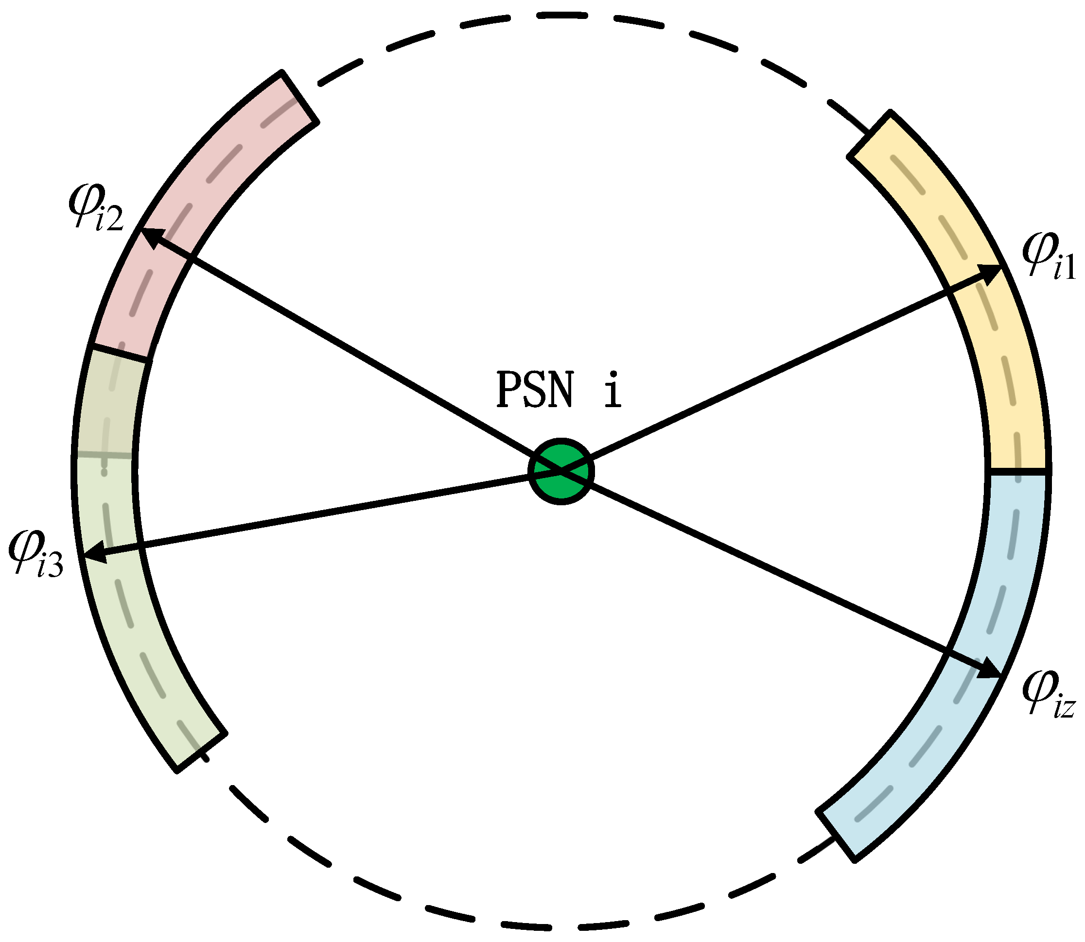
The traditional virtual force algorithm considers the interaction forces between nodes in Euclidean space. Differently from the traditional virtual force algorithm, we consider the interaction force between isomorphic antennas on the charging nodes. Assume that the azimuth distribution of the antenna on the $B_i\mathrm{th}$ charging node is shown in Figure 4, which are ${\phi }_{i,1},{\phi }_{i,2},\dots ,{\phi }_{i,z}$ respectively. Their distribution is not the coordinates in the Euclidean space, but the angle distribution on the ring structure and can be circulated.

The dotted line in the Figure 4 represents the circle with an azimuth, the position pointed at by the arrow represents a different azimuth, and the band interval near the azimuth represents the threshold limit range of azimuth. Then, the distance $d_i^{u,v}$ between azimuth ${\phi }_{i,u}$ and azimuth ${\phi }_{i,v}$ is defined as

$$d_i^{u,v}=\left|{\phi }_{i,u}-{\phi }_{i,v}\right|$$

(15)

The force ${\overrightarrow{F}}_i^{u,v}$ between azimuth ${\phi }_{i,u}$ and azimuth ${\phi }_{i,v}$ is defined as

$${\overrightarrow{F}}_i^{u,v}=\left\{\begin{array}{cc}{\omega }_A(d_i^{u,v}-d_i^{th}),\hfill & \hfill if{d}_i^{u,v}>d_i^{th}\\ 0,\hfill & \hfill if{d}_i^{u,v}=d_i^{th}\\ {\omega }_R/d_i^{u,v},\hfill & \hfill if{d}_i^{u,v}<d_i^{th}\end{array}\right.$$

(16)

where ${\omega }_A$ and ${\omega }_R$ have the same meaning as Equation (14), and $d_i^{th}$ represents the virtual force threshold of the antenna on the PSN. By observing the overlap of the limited threshold range of each azimuth in Figure 4, the type of force between the azimuths can be judged. There is no coincidence area between azimuth ${\phi }_{i,1}$ and azimuth ${\phi }_{i,2}$, so there is attraction between them. Azimuth ${\phi }_{i,2}$ and azimuth ${\phi }_{i,3}$ overlap in some regions; i.e., there is repulsion between them. As a result, there is a tendency for the two azimuths to be adjusted to non-coincident states. Azimuth ${\phi }_{i,z}$ and azimuth ${\phi }_{i,1}$ are just in adjacent states, so there is no interacting force between them.

The other difference between the ring virtual force algorithm and the traditional virtual force algorithm is that only the adjacent azimuths interact with each other, while the non-adjacent azimuth angles do not interact with each other. For example, there is no force between azimuth ${\phi }_{i,1}$ and azimuth ${\phi }_{i,3}$, and the coincidence problem of their limited threshold range is not taken into account.

4.1.2. AVFPSO Algorithm

Particle swarm optimization is an algorithm developed by simulating the unpredictable motion of a flock of birds. It evolves around the advantages of sharing information in groups. The initial PSO algorithm was formed by adding the nearest neighbor speed match and adding the multidimensional search, in addition to considering the accelerated search based on distance. Then the PSO algorithm was optimized by introducing parameters such as inertia weight ${\omega }_P$. Suppose the $q\mathrm{th}$ particle in the population is denoted as $X_q=(x_{q,1},x_{q,2},\dots ,x_{q,W})$. The best position it has ever experienced, the value with the best fit, is represented by $pbes{t}_q=(p_{q,1},p_{q,2},\dots ,p_{q,W})$, where W denotes the dimension of the particle. The best adaptive value is given by

$$gbest=argmax\left(f\left(X_q\right)\right),q\in (1,2,\dots ,W)$$

(17)

The moving velocity of particle is denoted by $V_q(v_{q,1},v_{q,2},\dots ,v_{q,W})$. The updating formula of velocity and position is given by

$$V_{q,w}(t+1)={\omega }_P{V}_{q,w}\left(t\right)+c_1{r}_1(pbes{t}_{q,w}-x_{q,w}\left(t\right))+c_2{r}_2(gbes{t}_w-x_{q,w}\left(t\right))$$

(18)

and

$$x_{q,w}(t+1)=x_{q,w}\left(t\right)+V_{q,w}\left(t\right)$$

(19)

where $c_1$ and $c_2$ denote acceleration constants, and $r_1$ and $r_2$ denote random values within the range of [0,1].

When the PSO algorithm and ring virtual force algorithm are combined to solve the coverage problem, $f\left(X_q\right)$ in Equation (17) is replaced by $f(\varphi ,\theta )$ in Equation (9) to calculate the optimal fitness value $pbes{t}_q^{*}$ as follows:

$$pbes{t}_q^{*}=argmax\left(f(\varphi ,\theta )\right)$$

(20)

After completing the speed update, when updating the positions of particles, the azimuths of the antennas on the same PSN are adjusted by virtual force according to Equation (16).

4.2. QGES Algorithm for Problem 2

4.2.1. Solution of the Model

For the solution of the multi-node energy supply system model, the situation of the single-sensor node energy supply system is first considered. Similarly, each energy packet entering the sensor node receives fixed benefit $\epsilon$, and the waiting cost per unit time is c. The ultimate goal is to select the appropriate energy packet delivery rate, so as to minimize the total cost. Since the energy packet emission rate obeys the Poisson distribution with parameter $\lambda$, and the energy packet consumption of sensor nodes obeys the general distribution with parameter $\mu$, the queuing model of the energy supply system of the single-sensor node can be described as $M/G/1$. Assume that:

• $X_b$: represents the number of energy packets left in the node when the $b\mathrm{th}$ energy packet is consumed, and the consumed energy packet is numbered as b.
• $T_b$: represents the elapsed time (from the time when the $b\mathrm{th}$ energy packet is consumed) of the next ($\left(b+1\right)\mathrm{th}$) energy packet when the $b\mathrm{th}$ energy packet is consumed. $E\left(T_b\right)=\frac{1}{\mu }$, $E\left(T_b^2\right)=\frac{q}{{\mu }^2}$.
• $Y_b$: represents the number of new energy packets entering the node during the period when the $\left(b+1\right)\mathrm{th}$ energy packet is being consumed.

According to the queuing situation,

$$X_{b+1}=\left\{\begin{array}{cc}{Y}_b,\hfill & \hfill X_b=0,\\ X_b+Y_b-1,\hfill & \hfill X_b>0.\end{array}\right.$$

(21)

Let $d_{\beta }=P\left(Y_b=\beta \right)>0$; then, it can be proved that $\left\{X_b\right\}$ forms a Markov chain, which is generally called an embedded Markov chain. If ${p_{\alpha }}_{\beta }=P\left(X_{b+1}=\left.\beta \right|X_b=\alpha \right)$, $p_{0\beta }$ can be given as

$$p_{0\beta }=\left(X_{b+1}=\left.\beta \right|X_b=0\right)=P\left(Y_b=\beta \right)=d_{\beta }\left(\beta \ge 0\right)$$

(22)

When $X_b>0$,

$$p_{\alpha \beta }=P(Y_b=\beta +1-X_b|X_b=\alpha )=\left\{\begin{array}{cc}0,\hfill & \hfill \alpha >\beta +1\\ d_{\beta +1-\alpha },\hfill & \hfill \alpha \le \beta +1\end{array}\right.$$

(23)

Since the time $\left\{T_b,b\ge 1\right\}$ consumed by the energy packet is an independent identically distributed sequence of random variables, its public distribution function is denoted as $G\left(t\right)=P\left(T_b\le t\right)$. Then,

$$d_{\beta }=P\left(Y_b=\beta \right)={\int }_0^{\infty }P\left(\left.Y_b=\beta \right|T_b=t\right)dG\left(t\right)$$

(24)

where $P\left(\left.Y_b=\beta \right|T_b=t\right)$ represents the probability of $\beta$ new energy packets entering the system in time interval $\left(0,t\right)$. Since the energy packet arrives according to Poisson flow, we can get

$$P\left(\left.Y_b=\beta \right|T_b=t\right)=\frac{{\left(\lambda t\right)}^{\beta }}{\beta !}{e}^{-\lambda t}$$

(25)

Substituting Equation (25) into (24),

$$d_{\beta }={\int }_0^{\infty }\frac{{\left(\lambda t\right)}^{\beta }}{\beta !}{e}^{-\lambda t}dG\left(t\right)$$

(26)

Since $d_0=p_{00}>0$ and the states of the Markov chain are interconnected, this Markov chain is periodically irreducible. It satisfies

$$\begin{array}{cc}\hfill E\left(Y_b\right)& ={\sum }_{\beta =0}^{\infty }\beta d_{\beta }={\sum }_{\beta =0}^{\infty }\beta {\int }_0^{\infty }\frac{{\left(\lambda t\right)}^{\beta }}{\beta !}{e}^{-\lambda t}dG\left(t\right)\hfill \\ \hfill & ={\int }_0^{\infty }{\sum }_{\beta =0}^{\infty }\frac{{\left(\lambda t\right)}^{\beta -1}}{\left(\beta -1\right)!}{e}^{-\lambda t}\lambda tdG\left(t\right)={\int }_0^{\infty }\lambda tdG\left(t\right)\hfill \\ \hfill & =\lambda E\left(T_b\right)=\rho \hfill \end{array}$$

(27)

and

$$\begin{array}{cc}\hfill E\left(Y_b^2\right)& ={\sum }_{\beta =0}^{\infty }{\beta }^2{d}_{\beta }={\sum }_{\beta =0}^{\infty }{\beta }^2{\int }_0^{\infty }\frac{{\left(\lambda t\right)}^{\beta }}{\beta !}{e}^{-\lambda t}dG\left(t\right)\hfill \\ \hfill & ={\int }_0^{\infty }\left({\sum }_{\beta =0}^{\infty }\frac{{\left(\lambda t\right)}^{\beta }}{\left(\beta -2\right)!}+{\sum }_{\beta =1}^{\infty }\frac{{\left(\lambda t\right)}^{\beta }}{\left(\beta -1\right)!}\right)e^{-\lambda t}\lambda tdG\left(t\right)\hfill \\ \hfill & ={\int }_0^{\infty }\left[{\left(\lambda t\right)}^2+\lambda t\right]dG\left(t\right)={\lambda }^{2}E\left(T_b^2\right)+\lambda E\left(T_b\right)=q{\rho }^2+\rho \hfill \end{array}$$

(28)

It can be verified that the Markov chain is traversed when $\rho <1$, so there is a stationary distribution $\left\{p_{\beta },\beta \ge 0\right\}$ which satisfies

$$p_{\beta }={\sum }_{\alpha =0}^{\infty }{p}_{\alpha }{p}_{\alpha \beta }\left(\beta \ge 0\right)$$

(29)

Constructing the generating function to solve $p_{\beta }$, let $P\left(x\right)={\sum }_{\beta =0}^{\infty }{p}_{\beta }{x}^{\beta }$ and $D\left(x\right)={\sum }_{\beta =0}^{\infty }{d}_{\beta }{x}^{\beta }$. It can be obtained from Equations (22), (23) and (29) that when $\beta =0$, $x^0{p}_0=\left(p_0{d}_0+p_1{d}_0\right)x^0$; when $\beta =1$, $x{p}_1=\left(p_0{d}_1+p_1{d}_1+p_2{d}_0\right)x$; …; when $\beta =b$, $x^b{p}_b=\left(p_0{d}_b+p_1{d}_b+p_2{d}_{b-1}+\cdots +p_{b+1}{d}_0\right)x^b$. Add up all the equations to get

$$\begin{array}{cc}\hfill P\left(x\right)& =p_{0}D\left(x\right)+p_{1}D\left(x\right)+p_{2}xD\left(x\right)+p_3{x}^{2}D\left(x\right)+\cdots +p_b{x}^{b-1}D\left(x\right)+\cdots \hfill \\ \hfill & =\frac{D\left(x\right)}{x}(p_{0}x+p_{1}x+p_2{x}^2+p_3{x}^3+\cdots +p_b{x}^b+\cdots )\hfill \\ \hfill & =\frac{D\left(x\right)}{x}[p_0(x-1)+P\left(x\right)]\hfill \end{array}$$

(30)

Therefore, the generating function of energy packet quantity distribution in the system can be deduced as

$$P\left(x\right)=\frac{\left(1-x\right)p_{0}D\left(x\right)}{D\left(x\right)-x}$$

(31)

Since $D^{\prime }\left(x\right)={\sum }_{\beta =0}^{\infty }\beta d_{\beta }{x}^{\beta -1}$, $D^{\prime }\left(1\right)={\sum }_{\beta =0}^{\infty }\beta d_{\beta }=E\left(Y_b\right)=\rho$. $P\left(1\right)={\sum }_{\beta =0}^{\infty }{p}_{\beta }=1$ and $D\left(1\right)={\sum }_{\beta =0}^{\infty }{d}_{\beta }=1$. L ’Hopital’s rule is applied to Equation (31),

$$\underset{x\to 1}{lim}P\left(x\right)=\underset{x\to 1}{lim}\frac{\left(1-x\right)p_{0}D\left(x\right)}{D\left(x\right)-x}=\frac{p_0}{1-\rho }\Rightarrow p_0=1-\rho$$

(32)

Substituting Equation (32) into (31),

$$P\left(x\right)=\frac{\left(1-x\right)\left(1-\rho \right)D\left(x\right)}{D\left(x\right)-x}$$

(33)

Combining Equations (27) and (28),

$$D^{″}\left(1\right)={\sum }_{\beta =0}^{\infty }\left({\beta }^2{d}_{\beta }-\beta d_{\beta }\right)=E\left(Y_b^2\right)-E\left(Y_b\right)=q{\rho }^2$$

(34)

With Equations (34) and (31), applying L ’Hopital’s rule twice more, the average number of energy packets in the system can be obtained as

$$\begin{array}{cc}\hfill \Gamma \left(\rho \right)& =E\left(X_b\right)=P^{\prime }\left(1\right)={\left.{\left[\frac{\left(1-x\right)\left(1-\rho \right)D\left(x\right)}{D\left(x\right)-x}\right]}^{\prime }\right|}_{x=1}\hfill \\ \hfill & =\left(1-\rho \right)\frac{-2{\left[D^{\prime }\left(1\right)\right]}^2+2D^{\prime }\left(1\right)+D^{″}\left(1\right)}{2{\left[D^{\prime }\left(1\right)-1\right]}^2}=\rho +\frac{q{\rho }^2}{2\left(1-\rho \right)}\hfill \end{array}$$

(35)

In the single-node power supply system with the queuing model $M/G/1$, the cost minimization problem of a single-node power supply system can be described as

$$min\left[c\Gamma \left(\rho \right)-\epsilon \lambda \right]=min\left[\rho +\frac{q{\rho }^2}{2\left(1-\rho \right)}-\epsilon \lambda \right]$$

(36)

where $\lambda$ satisfies $0\le \lambda <\mu$.

Since Equation (36) is a differentiable strictly convex function, ${\Gamma }^{\prime }\left(\lambda \right)$ represents the first derivative of $\Gamma \left(\rho \right)$ with respect to $\lambda$, which can be given as

$${\Gamma }^{\prime }\left(\lambda \right)=\frac{1}{\mu }+\frac{q\left(2\mu -\lambda \right)\lambda }{2\mu {\left(\mu -\lambda \right)}^2}$$

(37)

Therefore, the optimal arrival rate ${\lambda }^{*}$ satisfies

$$\left\{\begin{array}{cc}c{\Gamma }^{\prime }\left({\lambda }^{*}\right)-\epsilon =0,\hfill & \hfill {\lambda }^{*}>0\\ c{\Gamma }^{\prime }\left({\lambda }^{*}\right)=\frac{c}{\mu },\hfill & \hfill {\lambda }^{*}=0\end{array}\right.$$

(38)

Combining Equations (38) and (37),

$$\frac{1}{\mu }+\frac{q\left(2\mu -{\lambda }^{*}\right){\lambda }^{*}}{2\mu {\left(\mu -{\lambda }^{*}\right)}^2}=\frac{\epsilon }{c}\left({\lambda }^{*}>0\right)$$

(39)

$\epsilon$ is a fixed value satisfying $\epsilon >0$, and ${\lambda }^{*}\left(\epsilon \right)$ is the optimal arrival rate. The solution of Equation (39) can be obtained as

$${\lambda }^{*}\left(\epsilon \right)=\mu -\mu \sqrt{\frac{q}{q+2\mu \epsilon /c-2}}\left({\lambda }^{*}>0\right)$$

(40)

Due to $0\le \lambda <\mu$, the optimal arrival rate of the energy packets is

$${\lambda }^{*}\left(\epsilon \right)=max\left\{0,\mu -\mu \sqrt{\frac{q}{q+2\mu \epsilon /c-2}}\right\}$$

(41)

From the system model of Equations (11) and (12), the problem of minimizing cost for multi-node energy supply system can be described as

$$f^{*}\left(\stackrel{\rightharpoonup }{\lambda }\right)=min{\sum }_{a=1}^A{c}_a{\Gamma }_a\left({\lambda }_a\right)$$

(42)

subject to

$${\sum }_{a=1}^A{\lambda }_a=\Lambda \left(0\le {\lambda }_a<{\mu }_a,a=1,2,\cdots ,A\right)$$

(43)

According to the generalized Lagrangian multiplier method, Equation (42) satisfies Equation (38) for each sensor node a and partial benefit $\epsilon$. Therefore, the optimal arrival rate similar to the single node can be obtained as

$${\lambda }_a^{*}\left(\epsilon \right)=max\left\{0,{\mu }_a-{\mu }_a\sqrt{\frac{q}{q+2{\mu }_a\epsilon /c_a-2}}\right\}$$

(44)

where ${\sum }_{a=1}^A{\lambda }_a^{*}\left(\epsilon \right)=\Lambda$. Since $\Lambda >0$, there is at least one solution ${\lambda }_1^{*}\left(\epsilon \right)>0$. Then, ${\mu }_1-{\mu }_1\sqrt{\frac{q}{q+2{\mu }_1\epsilon /c_1-2}}>0$; that is, $\epsilon >\frac{c_1}{{\mu }_1}$. In this case, ${\sum }_{a=1}^A{\lambda }_a^{*}\left(\epsilon \right)$ is a strictly increasing function of $\epsilon$. Thus, there is one and only one ${\epsilon }^{*}$, such that ${\sum }_{a=1}^A{\lambda }_a^{*}\left({\epsilon }^{*}\right)=\Lambda$. If $\epsilon >\frac{c_a}{{\mu }_a}$, ${\lambda }_a^{*}\left(\epsilon \right)>0$. Therefore, when $h<a$, ${\lambda }_h^{*}\left(\epsilon \right)>0$, which means that under the equilibrium state of the system, the former a sensor nodes obtain energy packets according to the arrival rate of ${\lambda }_a^{*}\left(\epsilon \right)$ to be charged. Other sensor nodes are not selected because of low energy efficiency and insufficient energy. Therefore, in the designed model of multi-node power supply system, $\epsilon >\frac{c_A}{{\mu }_A}$ needs to be set for supplying energy to all active sensors.

In the multi-node energy supply system with queuing model $M/G/1$ of each sensor node, the optimal arrival rate of each node energy packet can be obtained as

$${\lambda }_a^{*}=\left({\mu }_a-{\mu }_a\left.\sqrt{\frac{q}{q+2{\mu }_a{\epsilon }^{*}/c_a-2}}\right|{\sum }_{a=1}^A{\lambda }_a^{*}\left({\epsilon }^{*}\right)=\Lambda \right),{\epsilon }^{*}>\frac{c_A}{{\mu }_A}$$

(45)

In this case, the lowest cost of the energy supply system is

$$f^{*}\left(\stackrel{\rightharpoonup }{\lambda }\right)={\sum }_{a=1}^A{c}_a\left[1-\sqrt{\frac{q}{q+2{\mu }_a{\epsilon }^{*}/c_a-2}}+\frac{q{\left(1-\left.\sqrt{\frac{q}{q+2{\mu }_a{\epsilon }^{*}/c_a-2}}\right|\right)}^2}{2\sqrt{\frac{q}{q+2{\mu }_a{\epsilon }^{*}/c_a-2}}}\right]$$

(46)

where ${\sum }_{a=1}^A{\lambda }_a^{*}\left({\epsilon }^{*}\right)=\Lambda$ and ${\epsilon }^{*}>\frac{c_A}{{\mu }_A}$.

4.2.2. Model Analysis

When building the energy supply system model, it assumes that the energy consumption random process of sensor nodes follows the general distribution with parameter $\mu$. It satisfies $E\left(T_b\right)=\frac{1}{\mu }$ and $E\left(T_b^2\right)=\frac{q}{{\mu }^2}$. When $q=2$, $D\left(T_b\right)=\frac{1}{{\mu }^2}$, which means that the node energy consumption process is simplified to a negative exponential distribution. Then

$${\lambda }_a^{*}\left(\epsilon \right)={\mu }_a-\sqrt{\frac{{\mu }_a{c}_a}{\epsilon }}\left(\epsilon >\frac{c_a}{{\mu }_a}\right)$$

(47)

Combining ${\sum }_{a=1}^A{\lambda }_a^{*}\left(\epsilon \right)=\Lambda$,

$$\sqrt{\epsilon }=\frac{{\sum }_{a=1}^A\sqrt{{\mu }_a{c}_a}}{{\sum }_{a=1}^A{\mu }_a-\Lambda }$$

(48)

In the multi-node power supply system with each sensor node queuing model $M/M/1$, the equilibrium solution can be obtained as

$${\lambda }_a^{*}={\mu }_a-\frac{\sqrt{{\mu }_a{c}_a}}{{\sum }_{a=1}^A\sqrt{{\mu }_a{c}_a}}\left({\sum }_{a=1}^A{\mu }_a-\Lambda \right)$$

(49)

When $q=1$, $D\left(T_b\right)=0$. In this case, the energy consumption time of the sensor node follows the deterministic distribution; when $1<q<2$, it follows the $\frac{1}{q-1}$-order Irish distribution. By analyzing the random process of node energy consumption in WRSNs, the random distribution which minimizes the cost of energy supply system is gotten under the same system parameters. According to this conclusion, the energy consumption time distribution of sensor nodes can be designed by adding a sleep mechanism.

4.3. Realization of the TPEM scheme

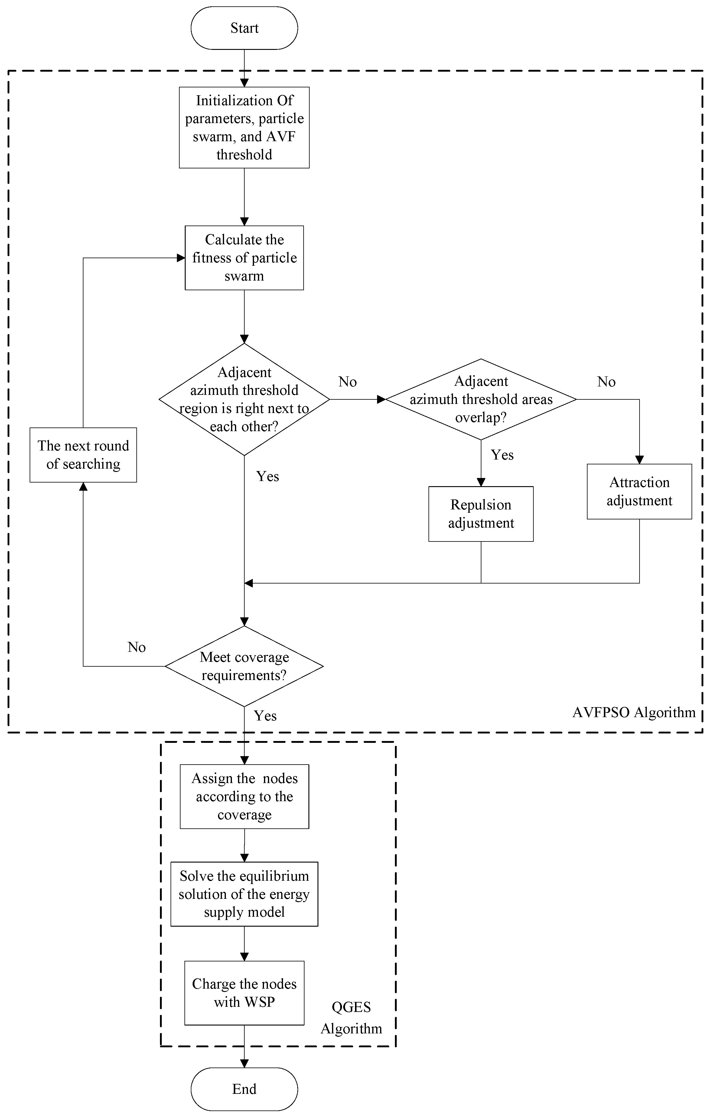
The AVFPSO algorithm and QGES algorithm are combined to realize the TPEM scheme for WRSNs, as shown in Figure 5.

In the first phase of the TPEM scheme, the threshold interval of antenna azimuth on the same PSN is determined by the initialization of AVFPSO algorithm. The initial particle swarm is then generated within the range of each parameter. After that, the fitness of each particle swarm is calculated and iterated. Then we determine the relationship between the position and the threshold. If the adjacent azimuth threshold interval overlaps, the azimuth is adjusted by repulsion. If the adjacent azimuth threshold interval diverges, the azimuth is adjusted by attraction. If the adjacent azimuth threshold intervals happen to be next to each other, the next step is entered. The search for the maximum coverage is completed by the cross-iterative updating of two particle swarms. Finally, the optimal solution of azimuth and tilt is obtained to achieve the area coverage. The pseudocode of AVFPSO algorithm is described in Algorithm 1.

Algorithm 1: AVFPSO algorithm.

After the completion of the first phase, the TPEM scheme executes the QGES algorithm in the second phase to charge sensor nodes. The parameter information of nodes ${\mu }_a$, $c_a$, and q in the coverage area is obtained by the PSN. Random flow of energy packets with arrival rate $\Lambda \left(0<\Lambda <{\sum }_{a=1}^A{\mu }_a\right)$ is generated from the PSN. The arrival rate ${\lambda }_a^{*}$ of energy packets received by each sensor node is calculated according to Equation (45). ${\lambda }_a^{*}$ is taken as the weight of sensor node a, and the PSN adopts the smooth weighted polling (SWP) algorithm to provide energy packets for each sensor node. The pseudocode of QGES algorithm is described in Algorithm 2.

Algorithm 2: QGES algorithm.

5. Simulations and Comparisons

5.1. Parameter Settings

In the validation of the AVFPSO algorithm, COST-231 transmission model [21] was selected to calculate the path loss $L_{i,j}$. The adjustable parameters were antenna azimuth $objective:maxf(\varphi ,\theta )$ and tilt $objective:maxf(\varphi ,\theta )$ with the effective range $[0,2\pi )$. The DSNPSO algorithm [26], a modified PSO algorithm suitable for directed sensor networks, was selected as the comparison algorithm. In the simulation, real data with terrain height in real environment were used to verify the effectiveness of the AVFPSO algorithm. The parameters are described below in

Table 1. Specifications of the parameters of the AVFPSO algorithm.

Parameter Name	Meaning	Value
$f_0$	Antenna operating frequency	2600 MHz
$T{h}_{RSRP}$	Receiving signal strength threshold	−88 dBm
$C_M$	Model correction factor	3 dBm
$G_m$	Antenna reverse radiation	32 dBm
$SL{A}_V$	Lateral lobe attenuation	32 dBm
$G_{max}$	Maximum antenna gain	18 dBm
$N_p$	Particle swarm number	10, 20
$N_t$	Iterations	100
$C_1$	Acceleration factor 1	1.494
$C_2$	Acceleration factor 2	1.494
${\omega }_P$	Inertia weight	0.8
${\omega }_A$	Coefficient of attraction	1
${\omega }_R$	Coefficient of repulsion	600

.

In the validation of the QGES algorithm, the energy packet consumption rate of sensor node determined the operating efficiency of the network element. Parameter $q=\left\{2,\frac{3}{2},1\right\}$ was set to simulate the energy consumption interval obeying negative exponential distribution, 2-order Irish distribution, and deterministic distribution respectively. We set the number of sensor nodes with charging requirements as $A=3$ and the energy consumption rate as $\mu =\left\{10,20,35\right\}$. The energy packet generation rate of the PSN obeyed the Poisson distribution with parameter $\Lambda =50$. Each energy packet was consumed and converted into a network value for data acquisition, storage, or forwarding. The network value return of each energy packet was set as $\epsilon$. After the energy pack is charged into the sensor node, it needs to pay the waiting cost c before it is consumed. c is composed of the node energy storage space occupied by the energy pack and the reduction of power life. The cost of waiting can be translated into the loss of the data service and thus associated with the social welfare.

5.2. Numerical Simulation

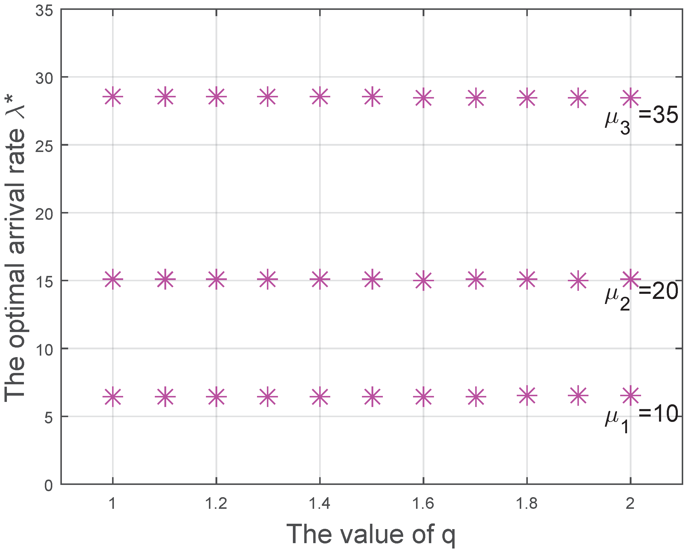
The corresponding parameters of QGES algorithm were put into Equation (45) for numerical calculation in MATLAB, and the results are shown as Figure 6. It depicts the relationship between the optimal energy packet allocation rate ${\lambda }^{*}$, the value of q, and energy consumption rate $\mu =\left\{10,20,35\right\}$ of the sensor node. When q increases from 1 to 2, it basically remains unchanged, indicating that different distribution of energy consumption interval has little influence on the optimal solution of the energy supply system. Obviously, the bigger $\mu$ is, the bigger the corresponding ${\lambda }^{*}$ is. It demonstrates that the nodes with higher energy consumption rate obtain more energy supply, which is consistent with normal rational cognition. However, under the optimal solution condition, the excess of the total energy consumption rate over total demand is not distributed uniformly among the nodes, but in a way that is proportional to the square root of their energy consumption rate. According to this conclusion, the design of energy supply strategy achieves the system cost minimization.

Based on Equation (46), the minimum cost of the energy supply system can be obtained with the energy consumption rate $\mu =\left\{10,20,35\right\}$. Figure 7 depicts the trend of the system minimum cost with the value q. $q=1$ represents the energy consumption time interval of the nodes following the deterministic distribution; $1<q<2$ represents the nodes following the $\frac{1}{q-1}$-order Irish distribution; and $q=2$ represents the nodes following the negative exponential distribution. From Figure 7, the minimum cost of the energy supply system increases with the increase of the value q. In other words, the system cost is the lowest when the node energy consumption time interval follows the deterministic distribution. Therefore, when designing the working scheme of sensor nodes, making the energy dissipation interval obey the random distribution with as small a variance as possible should be considered. Finally, maximize the social welfare of the system.

5.3. System Simulation

Figure 8 shows the actual network deployment map, where the yellow circle represents the location of the PSN. Other colors represent different actual terrain, such as green for forests and blue for rivers. Three directional charging antennas are configured on the yellow PSN nodes. This scenario contains 23 PSNs and the number of covered assessment sampling points is 62,730.

Firstly, the number of particle swarms was set to 10. As shown in Figure 9, the coverage implemented by AVFPSO algorithm was higher than that of DSNPSO algorithm in the whole iteration running interval. The AVFPSO algorithm also converged faster. Then we increased the number of particle swarms to 20. As shown in Figure 10, similarly to the previous results, the AVFPSO algorithm was still better than DSNPSO in terms of overall coverage performance and algorithm convergence. In the case of a larger particle swarm, the gap between the two was slightly larger than before. By comparing the AVFPSO algorithm with 10 particles and the DSNPSO algorithm with 20 particles, it can be observed that the performance of AVFPSO algorithm was still better than that of DSNPSO algorithm, even if the number of particle swarms was small. It means that the AVFPSO algorithm can get a faster search speed with the aid of virtual force algorithm.

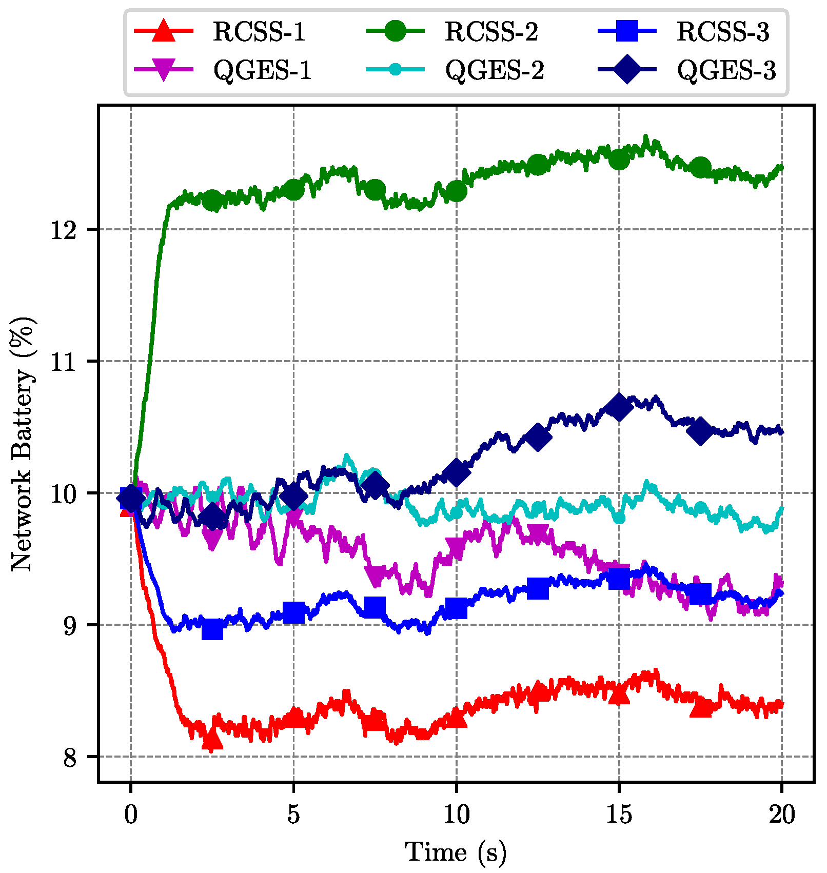
A real-time demand scheduling scheme (RCSS) [26] has been selected for a comparison of QGES algorithms. As shown in Figure 11, the Y-coordinate indicates the total electric quantity of the system. If the power is 0, it means that the system cannot work normally due to the power failure of one or more sensor nodes. Both algorithms start with the same initial electric quantity. The electric quantity obtained by each node is not uniform. When the electric quantity of some nodes is too low, the RCSS algorithm charges them to ensure the normal operation of the system. QGES algorithm is a balanced charging method based on the strategy of each node. The power of the system decreases slowly in a wave mode, indicating that each node in the network can maintain a relatively balanced power. As shown in Figure 12, within a short time after the system is started, the total power of the network charged by the RCSS algorithm decreases significantly. Overall, the QGES algorithm allows the system to maintain a higher power level than RCSS, allowing the network to operate for longer periods with the same amount of power.

6. Conclusions

The laying of 5G networks provides a foundation for future scenarios where things are connected. As the ends and edges of the Internet, WSNs provide massive data for the core network and reduce resource costs, such as manpower and equipment. The main constraint to the applications of WSNs is energy supply. In this paper, a TPEM scheme based on virtual force and the queuing game is proposed to extend the life cycles of WRSNs effectively. In the first phase, according to the position distribution characteristics of multiple antennas on the nodes, the AVFPSO algorithm was designed to achieve the coverage of the target area by solving the optimal azimuth and tilt. By using the virtual force to pull particles and by adjusting the optimal direction, the optimization algorithm can jump out of the local optimal solution and converge to the global optimal solution more quickly. After the coverage is completed, the limited energy is divided into energy packets and the queuing game theory is used to construct the energy supply system model. By solving the optimal energy supply strategy at the minimum cost, the QGES algorithm is designed to realize the optimal resources allocation of WRSNs. The change of system cost was analyzed with different random distributions of the energy consumption interval of nodes. The results show that the smaller the variance of the random distribution is, the lower the cost of the energy supply system—that is, the greater the social welfare that will be obtained. This conclusion can provide theoretical guidance for designing mechanisms such as node sleep scheduling. The system simulation results show that compared with the RCSS algorithm, the TPEM scheme achieves efficient energy management of WRSNs with lower total energy consumption in the same running time.

References

- Chernyshev, M.; Baig, Z.; Bello, O.; Zeadally, S. Internet of Things (IoT): Research, Simulators, and Testbeds. IEEE Internet Things J. 2018, 5, 1637–1647. [Google Scholar] [CrossRef]
- Li, H.; Xu, H.; Zhou, C.; Lü, X.; Han, Z. Joint Optimization Strategy of Computation Offloading and Resource Allocation in Multi-Access Edge Computing Environment. IEEE Trans. Veh. Technol. 2020, 69, 10214–10226. [Google Scholar] [CrossRef]
- Lu, X.; Wang, P.; Niyato, D.; Kim, D.I.; Han, Z. Wireless Charging Technologies: Fundamentals, Standards, and Network Applications. IEEE Commun. Surv. Tutor. 2016, 18, 1413–1452. [Google Scholar] [CrossRef] [Green Version]
- Amutha, J.; Sharma, S.; Nagar, J. WSN Strategies Based on Sensors, Deployment, Sensing Models, Coverage and Energy Efficiency: Review, Approaches and Open Issues. Wirel. Pers. Commun. 2020, 111, 1089–1115. [Google Scholar] [CrossRef]
- Saadi, N.; Bounceur, A.; Euler, R.; Lounis, M.; Bezoui, M.; Kerkar, M.; Pottier, B. Maximum Lifetime Target Coverage in Wireless Sensor Networks. Wirel. Pers. Commun. 2020, 111, 1525–1543. [Google Scholar] [CrossRef] [Green Version]
- Alibeiki, A.; Motameni, H.; Mohamadi, H. A new genetic-based approach for maximizing network lifetime in directional sensor networks with adjustable sensing ranges. Pervasive Mob. Comput. 2019, 52, 1–12. [Google Scholar] [CrossRef]
- Wang, Z.; Cao, Q.; Qi, H.; Chen, H.; Wang, Q. Cost-effective barrier coverage formation in heterogeneous wireless sensor networks. Ad Hoc Netw. 2017, 64, 65–79. [Google Scholar] [CrossRef]
- Sharmin, S.; Nur, F.N.; Islam, M.; Razzaque, M.A.; Hassan, M.M.; Alelaiwi, A. Target Coverage-Aware Clustering in Directional Sensor Networks: A Distributed Approach. IEEE Access 2019, 7, 64005–64014. [Google Scholar] [CrossRef]
- Zhu, X.; Li, J.; Zhou, M.; Chen, X. Optimal Deployment of Energy-Harvesting Directional Sensor Networks for Target Coverage. IEEE Syst. J. 2019, 13, 377–388. [Google Scholar] [CrossRef]
- Zhang, L.; Liu, T.T.; Wen, F.Q.; Hu, L.; Hei, C.; Wang, K. Differential Evolution Based Regional Coverage-Enhancing Algorithm for Directional 3D Wireless Sensor Networks. IEEE Access 2019, 7, 93690–93700. [Google Scholar] [CrossRef]
- Cao, B.; Zhao, J.; Lv, Z.; Liu, X. 3D Terrain Multiobjective Deployment Optimization of Heterogeneous Directional Sensor Networks in Security Monitoring. IEEE Trans. Big Data 2019, 5, 495–505. [Google Scholar] [CrossRef]
- Moraes, C.; Myung, S.; Lee, S.; Har, D. Distributed Sensor Nodes Charged by Mobile Charger with Directional Antenna and by Energy Trading for Balancing. Sensors 2017, 17, 122. [Google Scholar] [CrossRef] [PubMed] [Green Version]
- Na, W.; Park, J.; Lee, C.; Park, K.; Kim, J.; Cho, S. Energy-Efficient Mobile Charging for Wireless Power Transfer in Internet of Things Networks. IEEE Internet Things J. 2018, 5, 79–92. [Google Scholar] [CrossRef]
- Xu, W.; Liang, W.; Jia, X.; Xu, Z.; Li, Z.; Liu, Y. Maximizing Sensor Lifetime with the Minimal Service Cost of a Mobile Charger in Wireless Sensor Networks. IEEE Trans. Mob. Comput. 2018, 17, 2564–2577. [Google Scholar] [CrossRef]
- Tian, M.; Jiao, W.; Liu, J. The Charging Strategy of Mobile Charging Vehicles in Wireless Rechargeable Sensor Networks with Heterogeneous Sensors. IEEE Access 2020, 8, 73096–73110. [Google Scholar] [CrossRef]
- Jiang, J.R.; Liao, J.H. Efficient Wireless Charger Deployment for Wireless Rechargeable Sensor Networks. Energies 2016, 9, 696. [Google Scholar] [CrossRef] [Green Version]
- Li, L.; Dai, H.; Chen, G.; Zheng, J.; Dou, W.; Wu, X. Radiation Constrained Fair Charging for Wireless Power Transfer. ACM Trans. Sens. Netw. 2019, 15, 1–33. [Google Scholar] [CrossRef]
- Lin, C.; Wei, S.; Deng, J.; Obaidat, M.S.; Song, H.; Wang, L.; Wu, G. GTCCS: A Game Theoretical Collaborative Charging Scheduling for On-Demand Charging Architecture. IEEE Trans. Veh. Technol. 2018, 67, 12124–12136. [Google Scholar] [CrossRef]
- Yao, J.; Ansari, N. Caching in Energy Harvesting Aided Internet of Things: A Game-Theoretic Approach. IEEE Internet Things J. 2019, 6, 3194–3201. [Google Scholar] [CrossRef]
- Bell, C.; Jr, S. Individual versus Social Optimization in the Allocation of Customers to Alternative Servers. Manag. Sci. 1983, 29, 831–839. [Google Scholar] [CrossRef] [Green Version]
- Abhayawardhana, V.S.; Wassell, I.J.; Crosby, D.; Sellars, M.P.; Brown, M.G. Comparison of empirical propagation path loss models for fixed wireless access systems. In Proceedings of the 2005 IEEE 61st Vehicular Technology Conference, Stockholm, Sweden, 30 May–1 June 2005; Volume 1, pp. 73–77. [Google Scholar] [CrossRef]
- Navarro-Ortiz, J.; Romero-Diaz, P.; Sendra, S.; Ameigeiras, P.; Ramos-Muñoz, J.J.; López-Soler, J.M. A Survey on 5G Usage Scenarios and Traffic Models. IEEE Commun. Surv. Tutorials 2020, 22, 905–929. [Google Scholar] [CrossRef]
- Zou, Y.; Chakrabarty, K. Sensor Deployment and Target Localization Based on Virtual Forces. In Proceedings of the IEEE INFOCOM 2003, the 22nd Annual Joint Conference of the IEEE Computer and Communications Societies, San Franciso, CA, USA, 30 March–3 April 2003; pp. 1293–1303. [Google Scholar] [CrossRef] [Green Version]
- Jia, J.; Chen, J. An energy-balanced self-deployment algorithm based on virtual force for mobile sensor networks. Int. J. Sens. Netw. 2015, 19, 150–160. [Google Scholar] [CrossRef]
- Liu, S.; Zhang, R.; Shi, Y. Design of coverage algorithm for mobile sensor networks based on virtual molecular force. Comput. Commun. 2020, 150, 269–277. [Google Scholar] [CrossRef]
- Peng, S.; Xiong, Y. A New Sensing Direction Rotation Approach to Area Coverage Optimization in Directional Sensor Network. J. Adv. Comput. Intell. Intell. Inform. 2020, 24, 206–213. [Google Scholar] [CrossRef]
Figure 1.
A coverage and power supply system model of WRSNs.
Figure 2.
The relationship between antenna angle parameters and sampling point position.
Figure 3.
Energy supply system model.
Figure 4.
The azimuth distribution of the antenna on a power supply node (PSN).
Figure 5.
The flow of the TPEM scheme.
Figure 6.
The optimal allocation rate with a changing value of q.
Figure 7.
The trend of the system’s minimum cost while the value of q changes.
Figure 8.
The actual network deployment map.
Figure 9.
The coverage rate with 10 particles.
Figure 10.
The coverage rate with 20 particles.
Figure 11.
The electric quantity of the nodes with two algorithms.
Figure 12.
The electric quantity of the system with two algorithms.