Experimental Study of Substrate Limitation and Light Acclimation in Cultures of the Microalgae Scenedesmus obliquus—Parameter Identification and Model Predictive Control

Abstract

In this study, the parameters of a dynamic model of cultures of the microalgae Scenedesmus obliquus are estimated from datasets collected in batch photobioreactors operated with various initial conditions and light illumination conditions. Measurements of biomass, nitrogen quota, bulk substrate concentration, as well as chlorophyll concentration are achieved, which allow the determination of parameters with satisfactory confidence intervals and model cross-validation against independent data. The dynamic model is then used as a predictor in a nonlinear model predictive control strategy where the dilution rate and the incident light intensity are simultaneously manipulated in order to optimize the cumulated algal biomass production.

1. Introduction

Microalgae are often considered as a promising alternative for the production of renewable energy, particularly as a potential source of biofuels, in an attempt to replace fossil fuels with renewable alternatives; and/or as a method of capturing carbon dioxide, towards a more sustainable World [1,2,3]. The biofuels obtained from microalgae can be found in liquid form (bioethanol, biodiesel, vegetal oil) or gaseous form (biohydrogen or biosyngas) [4,5]. Other potentialities reside in providing proteins and other nutrients for animal feed and human food supplements [1,3,6,7] as well as other high-value molecules of pharmaceutical interest [1,7]. In this way, microalgae biomass and oil constitute a promising renewable feedstock for the emerging chemical technology and biotechnology industries. Therefore, there is a strong interest in developing dynamic models to better understand the microalgae-based processes and to develop control schemes that allow the optimal operation of these processes [8,9].

Nonetheless, in the way to continue the exploration of optimal operating conditions, some physiological properties of the microalgae related to their capacity to process light should be considered, using the current understanding of the photosynthetic process, along with our ability to efficiently exploit its properties. To improve culturing systems, the development of mathematical models capable of predicting photosynthetic productivity under dynamic conditions is crucial. Especially important is the adaptation process, due to the light-harvesting capacity of the photon flux, known as photoacclimation. Microalgae cultures can suffer a loss in biomass productivity due to a lack of illumination resulting from the darkening effect in the photobioreactor, or due to photoinhibition in the case of an excessive illumination. However, this loss can be alleviated by regulation of the light irradiance.

Globally speaking, the photosynthetic yield is affected by two key processes, which alter the impact of light conditions and nutrient supply over the culture. Photoinhibition is the first of them, which causes a decrease in the photosynthesis rate due to an excess of light, and later induces damage over some proteins in the photosynthetic apparatus [10]. Photoacclimation is the second, and can be defined as the process by which microalgae adapt their pigment composition to the photon flux density, also altering the photosynthesis rate.

A pioneer work can be found in [11,12,13], where the photoinhibition process is modeled at the level of the photosynthetic units inside the microalgae. The effect of photoinhibition is described through the photo-oxidative inactivation of these units, led by an excess of photon flux over the one required for photosynthesis, which denatures key proteins in the electron transfer chain [14,15]. This concept was used to explain the hysteresis effect found in P-I curves (photosynthesis rate vs. photon flux density), because photosynthetic rates measured with a succession of increasing irradiance levels are often higher than the rates measured with a series of decreasing irradiance.

For the production of microalgae in photobioreactors, the chemostat mode, i.e., equal inlet and outlet flows seems to be more profitable, because it allows prolonged stable operation, possibly at maximum productivity [16]. Microalgae photobioreactors are complex systems, mainly due to their nonlinear and time-varying behavior. In early literature, a model proposed for outdoor cultures [17] simulates biomass production, pH, growth rate, oxygen evolution, and carbon dioxide fixation rate.

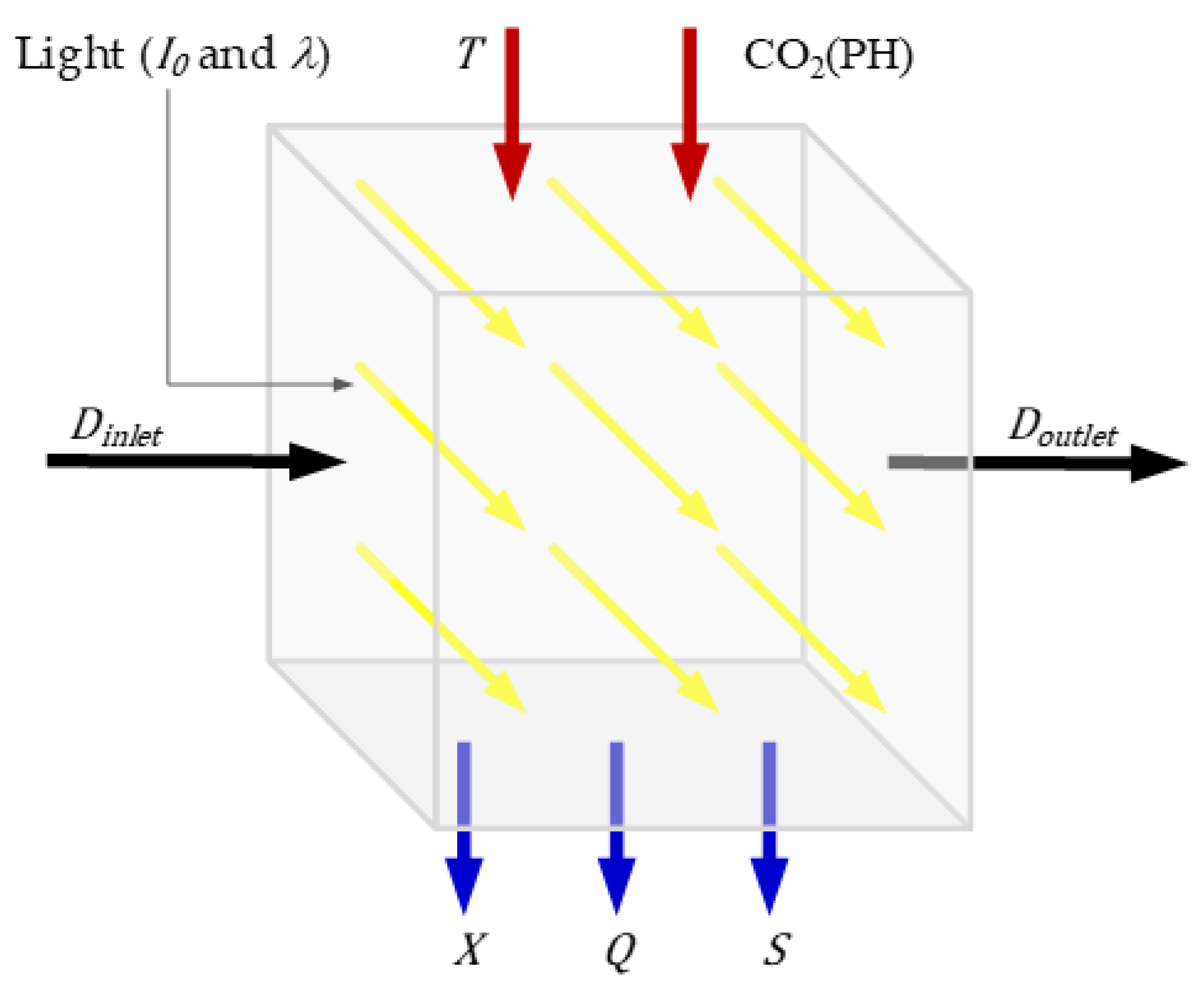
Microalgae modeling usually involves three basic states, accounting for biomass, substrate internal quota, and a substrate external concentration, respectively. Figure 1 illustrates some of the most common variables involved in a microalgae photobioreactor, either as inputs or outputs. An example of this kind of model can be found in [18], where a parameter identification is performed over batch cultures of Dunaliella tertiolecta strain. In addition, modeling of neutral lipids and carbohydrates quotas were introduced in [19] with a five-state model. A more complex mathematical representation considering eight state variables, in view of nitrogen and phosphorus as substrate limited sources, and comprising sugar and lipids concentration quotas was reported by [20]. Moreover, this model was used in an optimization problem to minimize the culture costs accounting for light, aeration, and cooling processes [21]. On the other hand, some research works followed a black-box modeling approach. In [22] an input-output adaptive identification based on artificial neural networks (ANN) was proposed for biomass control by adjusting the photon flux density (In [23], it is recommended to use the term photon flux density instead of light intensity—widely use in the literature, as it is technically more suitable. Further, it is advised to use the units [$\mathsf{\mu }\mathrm{mol}/{\mathrm{m}}^2\mathrm{s}$] for this magnitude, instead of [$\mathsf{\mu }\mathrm{E}/{\mathrm{m}}^2\mathrm{s}$], as the first one belongs to Le Système International (SI) of units). In [24], a Hammerstein–Wiener representation is used to develop an extremum seeking strategy.

One of the most frequently cited models is the one developed in [25], which accounts for the photoinhibition and shading effects inside the cultures. This model describes the dynamics of the three basic states ($X$, $Q$, and $S$), but incorporates a novel approach with a fourth conceptual variable named photoacclimation photon flux density, $I^{*}$, that represents the photon flux density at which the microalgae are currently physiologically acclimated. This model is presented with an analytical integration based on the average growth rate throughout the whole culture in [26]. The model of [25] is in a convenient form to be exploited for process control, particularly when the expression of the photoinhibition phenomenon is simplified and changed for a Haldane-inhibitory formulation. In [10] an equation is introduced to simulate the dynamics of chlorophyll, removing in this way the intermediate variable of photoacclimation photon flux density to represent the photoacclimation state of the culture. Instead, an expression for the chlorophyll concentration is formulated based on the incident light irradiance. Other modeling studies investigate the effect of other variables that affect microalgae growth, especially temperature [27].

In this study, we will focus attention on the model originally proposed in [25,26] and develop a parameter identification study for cultures of the microalgae Scenedesmus obliquus in batch photo-bioreactors. Our motivation is that, even if the models of [25,26] are largely accepted, their validation with experimental data is limited to a few case studies. In the current work, measurements of the biomass, intracellular substrate quota, extracellular substrate, and Chlorophyll concentrations are collected from nine batch experiments differing by their initial conditions and light exposition conditions. The parameters of a dynamic model are then estimated using a weighted least squares approach, and the uncertainty in the parameters is estimated based on the Fisher Information Matrix (FIM). Monte Carlo studies allow the model cross-validation against datasets not used in the identification procedure. Further, the dynamic model is exploited in a simulation study demonstrating the potential benefits of a Nonlinear Model Predictive Control (NMPC) for the optimization of the biomass production in a continuous photo-bioreactor, acting simultaneously on the dilution rate and the light intensity.

2. Model Description

In this section, we discuss a dynamic model describing photo-acclimation and photo-inhibition, originally proposed in [25,26]. This model uses the classical Droop expression [28] for substrate (S) uptake, internal quota (Q) evolution, and biomass (X) growth as basic building block and introduces a state variable called photon flux density of photoacclimation, $I^{*}$, which represents the intensity at which the culture is photoacclimated at a specific physiological level, rather than the actual photon flux density to which it is exposed.

To model the time evolution of this additional variable, expressions based on the Beer–Lambert law for the absorbance of light in the culture medium are proposed. An average light irradiation is computed, which is the photon flux density that affects the culture mass on average, $\overline{I}$. This parameter drives the dynamics of the acclimation phenomenon through a recall factor proportional to $\left(\overline{I}-I^{*}\right)$. A full model development description can be found in [25,26]. This model has been implemented in several occasions [20,21,24,27,29,30,31,32], sometimes including simplifications.

The mass balance model of a photobioreactor for the main species in liquid and gaseous phases (including, substrates, products, and biomass concentration) is given by the general model representation [33].

$$\frac{d\xi }{dt}=K{r}_x(.)+D\left({\xi }_{in}-\xi \right)-Q\left(\xi \right)+F$$

(1)

Taking the mathematical description of photo-acclimation into account and using appropriate kinetic expressions for $\rho$ and $\mu$, the mass balances for $X$, $S$ and $Q$ in a continuous stirred-tank reactor (CSTR) can be described as:

$$\dot{X}=\mu \left(X, Q,I_0\right)X-DX-RX$$

(2)

$$\dot{Q}=\rho \left(Q,S\right)-\stackrel{=}{\mu }\left(X,Q,I_0\right)\left(Q-Q_0\right)$$

(3)

$$\dot{S}=D{S}_{in}-\rho \left(Q,S\right)X-DS$$

(4)

$$\dot{I^{*}}=\mu \left(X, Q,I_0\right)\left[\overline{I}\left(I_0\right)-I^{*}\right]$$

(5)

where $D$ and $R$ denote, respectively, the dilution rate and the respiration rate; and $S_{in}$, the nutrient concentration in the feed. This model assumes Monod kinetics—at low and moderate media concentration, Andrews inhibition kinetics—at high media concentration, Droop model for internal nutrient cell quota, and light-limited/photo-initiated Haldane inhibition kinetics.

The remaining model parameters are calculated according to the following expressions. In Nomenclature,

Table A1. Variable and parameter nomenclature list.

Variable	Definition
$X$	Biomass bulk concentration	$\left[{\mathrm{g}}_{\mathrm{X}}/{\mathrm{m}}^3\right]$
$Q$	Nitrogen quota intracellular concentration	$\left[{\mathrm{g}}_{\mathrm{N}}/{\mathrm{g}}_{\mathrm{X}}\right]$
$S$	Nitrogen substrate bulk concentration	$\left[{\mathrm{g}}_{\mathrm{N}}/{\mathrm{m}}^3\right]$
$I^{*}$	Photon flux density acclimation	$\left[\mathsf{\mu }\mathrm{mol}/{\mathrm{m}}^2\mathrm{s}\right]$
Input	Definition
$I_0$	Photon flux density	$\left[\mathsf{\mu }\mathrm{mol}/{\mathrm{m}}^2\mathrm{s}\right]$
$D$	Dilution rate	$\left[{\mathrm{d}}^{-1}\right]$
$S_{in}$	Nitrogen concentration in the reactor inlet	$\left[{\mathrm{g}}_{\mathrm{N}}/{\mathrm{m}}^3\right]$
Parameter	Definition
Chlorophyll Parameters
$Chl$	Chlorophyll concentration	$\left[{\mathrm{g}}_{\mathrm{X}}/{\mathrm{m}}^3\right]$
$\theta$	Chlorophyll quota	$\left[{\mathrm{g}}_{\mathrm{Chl}}/{\mathrm{g}}_{\mathrm{X}}\right]$
$\delta$	Chlorophyll adaptation rate	$[-]$
$\overline{I}$	Average photon flux density throughout the culture	$\left[\mathsf{\mu }\mathrm{mol}/{\mathrm{m}}^2\mathrm{s}\right]$
Growth Kinetics Parameters
$\mu$	Specific growth rate	$\left[{\mathrm{d}}^{-1}\right]$
$\overline{\mu }$	Maximum specific growth rate	$\left[{\mathrm{d}}^{-1}\right]$
$\stackrel{=}{\mu }$	Average specific growth rate	$\left[{\mathrm{d}}^{-1}\right]$
Light Parameters
$\rho$	Nitrogen intake rate	$\left[{\mathrm{g}}_{\mathrm{N}}/{\mathrm{g}}_{\mathrm{X}}\mathrm{d}\right]$
$\overline{\rho }$	Maximum nitrogen intake rate	$\left[{\mathrm{g}}_{\mathrm{N}}/{\mathrm{g}}_{\mathrm{X}}\mathrm{d}\right]$
$k_s$	Substrate uptake half saturation constant	$\left[{\mathrm{g}}_{\mathrm{N}}/{\mathrm{m}}^3\right]$
$Q_l$	Maximum nitrogen quota	$\left[{\mathrm{g}}_{\mathrm{N}}/{\mathrm{g}}_{\mathrm{X}}\right]$
$Q_0$	Minimum nitrogen quota	$\left[{\mathrm{g}}_{\mathrm{N}}/{\mathrm{g}}_{\mathrm{X}}\right]$
Light Parameters
$I_{opt}$	Optimum photon flux density	$\left[\mathsf{\mu }\mathrm{mol}/{\mathrm{m}}^2\mathrm{s}\right]$
$k_{sI}$	Normalized growth half saturation constant	$\left[\mathsf{\mu }\mathrm{mol}/{\mathrm{m}}^2\mathrm{s}\right]$
$k_{sI}{}^{*}$	Growth half saturation constant	$\left[\mathsf{\mu }\mathrm{mol}/{\mathrm{m}}^2\mathrm{s}\right]$
$k_{iI}$	Photon flux density saturation constant over growth	$\left[\mathsf{\mu }\mathrm{mol}/{\mathrm{m}}^2\mathrm{s}\right]$
$\gamma$	Chlorophyll saturation function	$\left[{\mathrm{g}}_{\mathrm{Chl}}/{\mathrm{g}}_{\mathrm{N}}\right]$
$\overline{\gamma }$	Maximum chlorophyll saturation function	$\left[{\mathrm{g}}_{\mathrm{Chl}}/{\mathrm{g}}_{\mathrm{N}}\right]$
$k_{I^{*}}$	Chlorophyll saturation function constant	$\left[\mathsf{\mu }\mathrm{mol}/{\mathrm{m}}^2\mathrm{s}\right]$
Turbidity Parameters
$\xi$	Light attenuation rate light attenuation coefficient	$[-]$
$\lambda$	Optical depth	$\left[{\mathrm{m}}^{-1}\right]$
$L$	Culture depth	$\left[\mathrm{m}\right]$
$a$	Attenuation coefficient due to chlorophyll	$\left[{\mathrm{m}}^2/{\mathrm{g}}_{\mathrm{Chl}}\right]$
$b$	Attenuation coefficient due to biomass	$\left[{\mathrm{m}}^2/{\mathrm{g}}_{\mathrm{X}}\right]$
$c$	Attenuation coefficient due to background turbidity	$\left[{\mathrm{m}}^{-1}\right]$
$K_g$	Average photon flux density saturation function constant	$[-]$

contains a full description of the model nomenclature.

Specific Growth Rate

$$\mu =\stackrel{=}{\mu }\left(1-\frac{Q_0}{Q}\right)$$

(6)

$$\stackrel{=}{\mu }=\overline{\mu }\frac{\overline{I}}{ k_{sI}+\overline{I}+\left(\frac{{\overline{I}}^2}{ k_{iI}}\right)}$$

(7)

$$I_{opt}=\sqrt{k_{sI} k_{iI}}$$

(8)

$$k_{sI}=\frac{{k_{sI}}^{*}}{\theta } , \theta =\frac{Chl}{X}$$

(9)

$$\lambda =\xi L , \xi =aChl+bX+c$$

(10)

$$Chl = \gamma \left(I^{*}\right)XQ , \gamma \left(I^{*}\right)=\overline{\gamma }\frac{k_{I^{*}}}{k_{I^{*}}+I^{*}}$$

(11)

Nitrogen Uptake

$$\rho =\overline{\rho }\frac{S}{k_s+S}\left(1-\frac{Q}{Q_l}\right)$$

(12)

Average Photon Flux Density

$$\overline{I}=I_0\frac{K_g}{K_g+\lambda }$$

(13)

3. Materials and Methods

The microalgae strain used in this work is Scenedesmus obliquus (also known as Tetradesmus obliquus), a freshwater microalgae, first reported in [34]. The inoculum was obtained from the Culture Collection of Algae and Protozoa (CCAP 276/3A). The microalgae cultures are run into VWR^® 5 L borosilicate beakers, and their variables are monitored by measuring the biomass, nitrogen quota, substrate concentration, and chlorophyll ($Chl$) concentration with the techniques described in the following subsections.

3.1. Variable Measurement

3.1.1. Biomass Measurement

The standard off-line method for quantifying biomass concentration of the culture is the dry weight mass measurement [35]. The procedure requires several steps for cell separation, washing, and drying to a constant weight. The main drawback, however, is the lack of distinction between living and dead cellular material when taking the measurement.

Operation Procedure

• Place cellulose acetate membrane filters (Whatman^® $0.2 \mathsf{\mu }\mathrm{m}$ (Sigma-Aldrich, St. Louis, MI, USA)) inside an oven at 105 °C and leave them overnight.
• Retrieve the dried filters and allow them to cool down in a desiccator for 8 h. Weigh the chosen filter and record the value $W_{start}$.
• Extract a sample from the culture. Filter the sample using a vacuum pump; this leaves the biomass separated on the membrane aside from the medium.
• Dry the filter together with the algal biomass in a furnace at 105 °C until a constant weight is achieved and then cool in a desiccator for 20 min.
• Weight the sample on an analytical balance and record the value $W_{end}$.
• Determine the biomass weight as the difference between $W_{start}$ and $W_{end}$, with the corresponding factor adjustment.

$$DW=\frac{\left(W_{end}-W_{start}\right)}{V \left[mL\right]}$$

(14)

In this study, a Sartorius^® AZ214 M-Power Analytical Balance (Sartorius, Goettingen, Germany) was used, with a readability of ±0.0001 g and a repeatability of ±0.0003 g; while the volume of the samples was taken with a pipet of ±0.01 mL precision.

3.1.2. Quota Measurement

The nitrogen determination was carried out with a Shimadzu^® TOC-VCSN & TNM-1 (Shimadzu, Kyoto, Japan) instrument, which provides measurements over a wide range from 0.1 mg/L to 4000 mg/L of nitrogen.

Operation Procedure

• Take the sample from the medium culture into a 15 mL vial.
• Centrifuge it for 5 min at 5000 rpm. Remove the supernatant and gently shake the vial to dilute biomass. Use demineralized water to fill up to 15 mL.
• Repeat the previous step to wash the biomass and ensure a proper removal of substrate in the medium.
• Process the sample with the equipment to obtain the total nitrogen content ($TN$).

The intracellular quota $Q$ is then derived from total nitrogen measurements and biomass concentration $X$:

$$Q=\frac{TN}{X}$$

(15)

The measurement of nitrogen quota has a ±0.01 mg/L sensitivity.

3.1.3. Substrate Measurement

In order to quantify the nitrate (substrate) concentration in the medium, a spectrophotometry method is used [36]. When dissolved in water, nitrate absorbs UV light under 250 nm. Sample turbidity from organic material disturbs the absorbance measurement. To cope with this interference, two different measurements must be taken at specific wavelengths: 210 nm ($AB{S}_{210}$) and 270 nm ($AB{S}_{270}$). For the first determination, a peak is observed which contains the maximum nitrate absorption plus the so-called interference, whereas for the second one, only the effect of turbidity is considered. Accordingly, one can compute:

$$N_{OD}=AB{S}_{210}-AB{S}_{270}$$

(16)

where $N_{OD}$ corresponds to the nitrate concentration from the optical density measurement.

A Shimadzu^® UVmini-1240 spectrophotometer is used, with a sensitivity of ±0.1 for absorbance measurements. The relationship between absorbance and nitrate concentration is obtained by preparing several dilutions of a nitrate solution. The absorbance difference ($N_{OD}$) is then linearly correlated to the nitrate concentration, $S$:

$$S=C_s N_{OD}$$

(17)

where $C_s$ is a linear correlation coefficient. On-line measurements can also be implemented using a deuterium light source and a spectrometer, connected to a fiber optics probe. The light travels through the probe across the culture medium, where it is absorbed, and eventually reaches the spectrometer.

Operation Procedure

• Collect a 5 mL sample from the reactor.
• Centrifuge the sample over 5 min at 5000 rpm.
• Take out 4 mL of supernatant and introduce it into a spectrophotometer cuvette.
• Measure the absorbance with the spectrophotometer at 210 nm and 270 nm.
• Determine the concentration of the substrate according to the correlation curve.

A centrifugation step is accomplished before the absorbance measurement to eliminate the microalgae so that they do not interfere with the measurement. The volume samples are taken with a pipet of ±0.01 mL sensitivity.

3.1.4. Chlorophyll Measurement

For this propose, the extraction method described in [37] is followed, changing the filtering step for a centrifugation one to generate less turbidity and manage a smaller sample volume. Additionally, a step of mechanical grinding is used in order to improve the chlorophyll extraction from the microalgae, as reported in [38,39].

Operation Procedure

• Collect a 10 mL sample from the reactor in a 15 mL test tube.
• Centrifuge the sample over 5 min at 5000 rpm.
• Take out 9 mL of supernatant, add 3 mL of acetone and mix.
• Transfer the content to a 10 mL capsule of a ball mill.
• Add glass microspheres under 0.50 mm into the capsule, and shake it at 30 Hz for 20 min.
• Remove the capsule and transfer the content to a test tube.
• Fill the tube up to 10 mL of content adding acetone. This way the full content will be 90% acetone and 10% water, with the pigments solved in it.
• Centrifuge over for 5 min at 5000 rpm.
• Take out 4 mL of supernatant and transfer it to a 10 mm glass cuvette for the spectrophotometer.
• Measure the absorption at 630, 647, 664, and 750 nm.

To consider that the extraction is properly executed, the measurement at 750 nm should be less than 0.010, while the absorption peak at 664 nm should not be higher than 1.000. The correlation between the absorbance and the concentration of the pigments is made with the formulas from [40] for extraction with 90% acetone solvent. This sample should be processed just after being taken. Otherwise, after the first centrifugation and supernatant extraction, it can be preserved at −18 °C for up to one month.

3.1.5. Irradiance Measurement

Quantum sensors measure photosynthetically active radiation (PAR)—also named as photosynthetic photon flux density (PPFD)—which is the photon flux density in the spectral range (wave band) of solar radiation from 400–700 nm that photosynthetic organisms are able to use in the process of photosynthesis. An Apogee^® MQ-200 Quantum Sensor (Apogee, Santa Monica, CA, USA) ($\pm 1{ \mathsf{\mu }\mathrm{mol} \mathrm{m}}^{-2}{ \mathrm{s}}^{-1}$) was used to measure the light received by the culture.

3.2. Cell Culture and Medium Preparation

All cultures are maintained in heat-sterilized (121 °C over 20 min) modified Bold’s Basal Medium (BBM, see

Table 1. Bold’s Basal Medium (BBM) modified formula.

Formula	Concentration [g/L]		Concentration [g/L]
$\mathrm{NaCl}$	0.025	micro-nutrients 1
${\mathrm{MgSO}}_4·7{\mathrm{H}}_2\mathrm{O}$	0.075	${\mathrm{ZnSO}}_4·7{\mathrm{H}}_2\mathrm{O}$	8.829
${\mathrm{CaCl}}_2·2{\mathrm{H}}_2\mathrm{O}$	0.025	${\mathrm{MnCl}}_2·4{\mathrm{H}}_2\mathrm{O}$	1.441
${\mathrm{NaNO}}_3$	0.750	${\left({\mathrm{NH}}_4\right)}_6{\mathrm{Mo}}_7{\mathrm{O}}_{24}·4{\mathrm{H}}_2\mathrm{O}$	6.093
${\mathrm{K}}_2{\mathrm{HPO}}_4$	0.075	${\mathrm{CuSO}}_4·5{\mathrm{H}}_2\mathrm{O}$	1.571
${\mathrm{KH}}_2{\mathrm{PO}}_4$	0.176	${\mathrm{CoCl}}_2·6{\mathrm{H}}_2\mathrm{O}$	0.400
micro-nutrients 1	1 mL	${\mathrm{H}}_3{\mathrm{BO}}_3$	11.439
micro-nutrients 2	1 mL	micro-nutrients 2
micro-nutrients 3	1 mL	$\mathrm{EDTA}.{\mathrm{Na}}_2$	63.651
		$\mathrm{KOH}$	31.026
		micro-nutrients 3
		${\mathrm{FeSO}}_4·7{\mathrm{H}}_2\mathrm{O}$	4.976
		${\mathrm{H}}_2{\mathrm{SO}}_4 \mathrm{concentrated}$	10 mL/L
		Vitamins
		Vitamin B1 (thiamine $HCl$)	8.934
		Vitamin H (biotine)	0.025
		Vitamin B12 (cyanocobalamine)	0.018

) at an initial pH value of 6.8 [41]. Prior to photobioreactor inoculation, the cultures were kept in an exponential growth phase for at least one week in Erlenmeyer flasks with constant agitation (250 rpm) and continuous light supply—no dark cycle—with constant photon flux density in the range $100–250{ \mathsf{\mu }\mathrm{mol} \mathrm{m}}^{-2}{ \mathrm{s}}^{-1}$.

3.3. Laboratory Scale Process

The photobioreactors used are cylindrical VWR^® (VWR International, Radnor, PA, USA) borosilicate glass beakers of 5 L with 17 cm in diameter with covers made of acrylic glass. These covers allow access to inoculation, culture sampling, nutrient addition, gas evacuation, and carbon dioxide injection. In all the conducted experiments, the total sample volume extracted was under 10% of the initial culture volume, a condition to be met so as to neglect the volume changes. The temperature was maintained in the range 22–24 °C thanks to a water bath which was adjusted manually at regular time intervals.

In autotrophic conditions, microalgae need light for their photosynthetic growth as an energy source, carbon dioxide as carbon source, as well as mineral nutrients such as nitrogen, phosphate, and sulfate sources. The carbon dioxide transfer, dissolution, and consumption lead to pH changes and, therefore, probes for pH (HAO SHI^® H-101 industrial online pH-meter) (HAO SHI, Taiwan) and carbon dioxide injections are installed to monitor and control the pH in the culture and to provide a carbon source to the microalgae. The pH is set at a constant value of 7.0. For mixing proposes, a magnetic bar of 70 mm long is positioned at the bottom of each reactor and moved by magnetic stirrers placed under the beaker at a constant speed of 250 rpm.

The effect of different wavelengths, especially the one of red/blue light with different ratios comparing against red, blue, and white light is reported in [42]. It is pointed out that light sources with red/blue lights in different ratios improve the growth rates of the microalgae. Other reports such as [43] support the same conclusion, aside from other effects on chlorophyll concentration or protein concentration changes. Hence, it is recommended to provide the microalgae with a wide variety of wavelengths, with emphasis on the red spectrum where the chlorophyll absorbs the light. The light source available for our experiments was a ROLEADRO^® (Shenzhen Houyi Energy Efficiency Co. Ltd., Shenzhen, China) Dual Channel Dimming 600 W full spectrum LED panel, composed of a combination of 7 different wavelengths mainly contained in the visible spectrum between 400–700 nm. (410, 450, 470, 440, 460, 580, 610, 630, 660, and 740 nm; 3000 k, 6500 k). This light source makes emphasis on the red and blue light bands, in an 8:1 ratio. The light panel is capable of generating up to $2000 {\mathsf{\mu }\mathrm{mol} \mathrm{m}}^{-2}{ \mathrm{s}}^{-1}$ from a close distance.

3.4. Experimental Design

The experiments are designed to provide informative datasets for parameter identification. As a first approach, operational ranges are defined for the substrate concentration, the photon flux density, and the biomass concentration inside the bioreactors, so as to observe various phenomena related to substrate uptake, biomass growth, photo-acclimation, and inhibition. Based on previous experimental observations (from literature and our research group expertise), it is known that microalgae cultures can run from very small concentrations of biomass, to a couple of thousands of milligrams per liter, while the substrate concentration can range from as low as zero to around a hundred milligrams per liter. Hence, the substrate concentration is varied in the experiments between high levels where no limitation occurs, to very low levels where microalgae are in a nutrient-limited environment, and where the Droop kinetics is active. Chlorophyll is directly proportional to the level of the nitrogen quota $Q$ and, at the same time, is highly dependent on the substrate concentration $S$. Some runs are therefore conducted with high substrate concentrations, trying to decouple this effect and making $Chl$ more dependent over the acclimation photon flux density, $I^{*}$. Last, the photon flux density operational range is explored at relatively low levels, especially over not so dense cultures, to collect data where microalgae do not express photoinhibition, and through the whole interval up to high levels, where photoinhibition can be detected and, at the same time, light penetration inside the dense culture is still possible.

In some of the culture runs, the operational variables are adjusted in a way that approaches the optimal conditions for biomass growth. As discussed in [44], this strategy tracks a performance path which is one of the ultimate goal of the model, and it is a good approach to excite the different kinetics and mechanisms along this path.

Table 2. Initial conditions, input variables values, and cultivation time for each culture run. (Physical units are defined in Table A1).

		Initial Conditions				Input Variables
Run	${\mathit{t}}_{\mathit{r}\mathit{u}\mathit{n}}$	${\mathit{X}}_0$	${\mathit{Q}}_0$	${\mathit{S}}_0$	${\mathit{I}}_0^{*}$	${\mathit{I}}_0$	$\mathit{D}$
1	14.6	10.1	0.025	33.2	100	100	0
2	14.6	12.3	0.030	36.5	100	150	0
3	15.5	30.7	0.061	41.3	200	200	0
4	15.5	18.7	0.069	39.4	200	250	0
5	13.1	60.3	0.026	44.8	100	220	0
6	13.1	76.7	0.023	47.5	100	350	0
7	11.0	225.0	0.016	49.9	250	520	0
8	11.0	255.0	0.017	52.0	150	600	0
9	13.3	183.8	0.022	42.6	200	750	0

shows the initial values of each state variable, the input variables values, and the cultivation time for each run.

4. Results

The collected experimental data can be used either for parameter identification, e.g., runs 1–4, 6–7, and 9, or for cross validation tests (runs 5 and 8 are therefore not exploited in the identification procedure). As illustrative examples, Figure 2 and Figure 3 display the four measured variables: biomass concentration, nitrogen internal quota, substrate concentration, and chlorophyll concentration, together with their 95% confidence intervals (estimated in the identification procedure as detailed in the next section) for the experimental runs 4 and 9. Moreover, these plots show a comparison with the model prediction based on the identified parameters (see

Table 3. Estimated parameters corresponding to Scenedesmus obliquus (physical units are defined in Table A1).

Parameter	Estimated Value	CV (%)	CI
$\overline{\mu }$	1.69	7.0	0.23
$k_s$	17.69	10.0	3.5
$Q_0$	0.0104	4.0	0.0008
$Q_l$	0.1172	8.2	0.0189
$\overline{\rho }$	0.0573	6.4	0.0072
${k_{sI}}^{*}$	1.36	17.3	0.46
$k_{iI}$	94.3	14.6	27.0
$R$	0.0779	2.1	0.0032
${\gamma }_{max}$	1.158	1.6	0.037
$k_{I^{*}}$	184	7.7	28
$a$	12.6	37.0	9.1
$b$	0.72	23.8	0.34
$c$	15.1	45.9	13.6
$K_g$	10.6	24.5	5.1

).

5. Model Parameter Identification

For the model chosen in this work, parameters can be grouped into two categories: growth parameters ($\overline{\mu }$, $k_S$, $Q_0$, $Q_l$, $\overline{\rho }$,$R$), and light parameters ($k_{sI}$, $k_{iI}$, ${\gamma }_{max}$, $k_{I^{*}}$, $a$, $b$, $c$, $K_g$). The first category actually contains parameters involved in many processes, like nutrient uptake kinetics, nutrient intracellular quota, respiration, and substrate-based growth kinetics, involving both factors, nutrient and light, respectively. The second category includes parameters relative to light absorption and scattering, and light acclimation. Roughly speaking, the identification of parameters in each category is favored by sets of data that excite one the most while diminishing the effects from the other category. Similarly, certain particular growth conditions are better for the determination of a certain parameter, e.g., internal quota lower and upper limits during starvation when nutrients are exhausted and during substrate repletion, respectively. The broad experimental conditions considered in this study contain a rich set of culture scenarios that excite the system in order to avoid potential parameter identifiability problems.

The model represented by Equations (2)–(5), can be expressed in a compact way as:

$$\dot{\xi }=f\left(\xi ,\theta ,t\right)$$

(18)

where $\xi \left(t\right)$ denotes the vector of state variables, and $\theta$ is the vector of the $n_p$ model parameters. Hence, using numerical integration, a solution of these nonlinear model equations provides a time profile of each state, which depends on the parameter set $\theta$.

$$y_{model}\left(t,\theta \right)=g\left(\xi ,\theta ,t\right)$$

(19)

where $y_{model}\left(t,\theta \right):{ℝ}_{+}\times {ℝ}^{n_p}\to {ℝ}^{n_y}$ stands for the output model prediction. Furthermore, the collected data at a time $t_i$ can be represented in a vector form as:

$$y\left(t_i\right)=y_{model}\left(t_i,{\theta }^{*}\right)+{\eta }_i,\hspace{1em}i=1\dots n_t$$

(20)

where ${\theta }^{*}$ represents the true value of the parameter vector, and $n_t$ is the number of observation times or measurements. This last expression links the measured value $y$ with the modeled result $y_{model}$. The idea is to try to match these two values through a multiparameter regression. The measurement errors are assumed to be independent, zero mean, and Gaussian.

$${\eta }_i ~ N\left(0, \mathsf{\Sigma }\right),\hspace{1em}i=1\dots n_t$$

(21)

Then, the identification of model parameters can be performed with a Weighted Least Squares (WLS) criterion, where the cost function $J\left(\theta \right)$ is formulated as:

$$J\left(\theta \right)={\displaystyle \sum }_{i=1}^{n_t}{\left(y\left(t_i\right)-y_{model}\left(t_i,\theta \right)\right)}^T{W}^{-1}\left(y\left(t_i\right)-y_{model}\left(t_i,\theta \right)\right)$$

(22)

and the weighting matrix can be selected as:

$$W=\left[\begin{array}{cccc}max{\left(y_1\right)}^2& 0& \cdots & 0\\ 0& max{\left(y_2\right)}^2& \cdots & 0\\ ⋮& ⋮& \ddots & ⋮\\ 0& 0& \cdots & max{\left(y_{n_y}\right)}^2\end{array}\right]$$

(23)

Note that the matrix $W$ scales each variable for differences in physical units and orders of magnitude. An estimation of the covariance matrix of the measurement noise can be done as

$$\widehat{\Sigma }={\widehat{\mathsf{\epsilon }}}^{2}W$$

(24)

where

$${\widehat{\mathsf{\epsilon }}}^2=\frac{J\left(\widehat{\theta }\right)}{n_y{n}_t-n_p}$$

(25)

with $n_y$ the number of model variables, $n_t$ the number of time samples, and $n_p$ the number of model parameters. The estimation of the parameters is obtained by minimizing the cost function $J\left(\theta \right)$.

$$\widehat{\theta }=\arg mi{n}_{\theta }J\left(\theta \right)$$

(26)

Various methods can be used to solve this minimization problem, which is nonconvex. For instance, a two-step procedure can be used where a genetic algorithm (GA)—i.e., ga in MATLAB^® (MathWorks, Natick, MA, USA)—is executed for the first step. With enough generations it allows locating a global minimum, avoiding falling into local minima. The second step can be achieved with the lsqnonlin function from MATLAB^®. Alternatively, the minimization of the cost function could be carried out using some local minimization method combined with a multi-start strategy which allows locating some of the local minima, and hopefully determining the global one. In this case, it is required to define a restricted parameter space and a set of initial parameter guesses, which can be obtained through a Latin Hypercube Sampling.

The Fisher Information Matrix, $FIM$, is then calculated as follows:

$$FIM={\displaystyle \sum }_{i=1}^{n_t}{\left(\frac{\partial y_{model}}{\partial \theta }\right)}_{\left(t_i,\widehat{\theta }\right)}^T{\widehat{\Sigma }}^{-1}{\left(\frac{\partial y_{model}}{\partial \theta }\right)}_{\left(t_i,\widehat{\theta }\right)}$$

(27)

where $\partial y_{model}/\partial \theta$ are the sensitivity matrices.

The analytical computation of these matrices for the model under consideration in this study is not an easy task. However, the sensitivity matrices can be obtained as a by-product of the lsqnonlin algorithm. The parameter covariance matrix is then approximated—assuming an unbiased estimator, as:

$$C_{\theta }\approx FI{M}^{-1}\left(\widehat{\theta },\widehat{\Sigma }\right)$$

(28)

The standard deviation ${\sigma }_j$ of the parameter estimates ${\widehat{\theta }}_j$ is obtained.

$${\sigma }_j=\sqrt{C_{\theta }{}_{jj}}$$

(29)

The 95% confidence intervals ($CI$) for each parameter can be calculated as $1.96\sigma ({\widehat{\theta }}_i)$. The coefficient of variation ($CV$) is then given by:

$$CV= \frac{\sigma \left({\widehat{\theta }}_i\right)}{{\widehat{\theta }}_i}$$

(30)

The computation of the confidence intervals can be easily achieved with the MATLAB^® command nlparci. An alternative procedure uses the outputs of nlinfit as inputs to nlparci. The parameters and their respective confidence intervals are listed in Table 3.

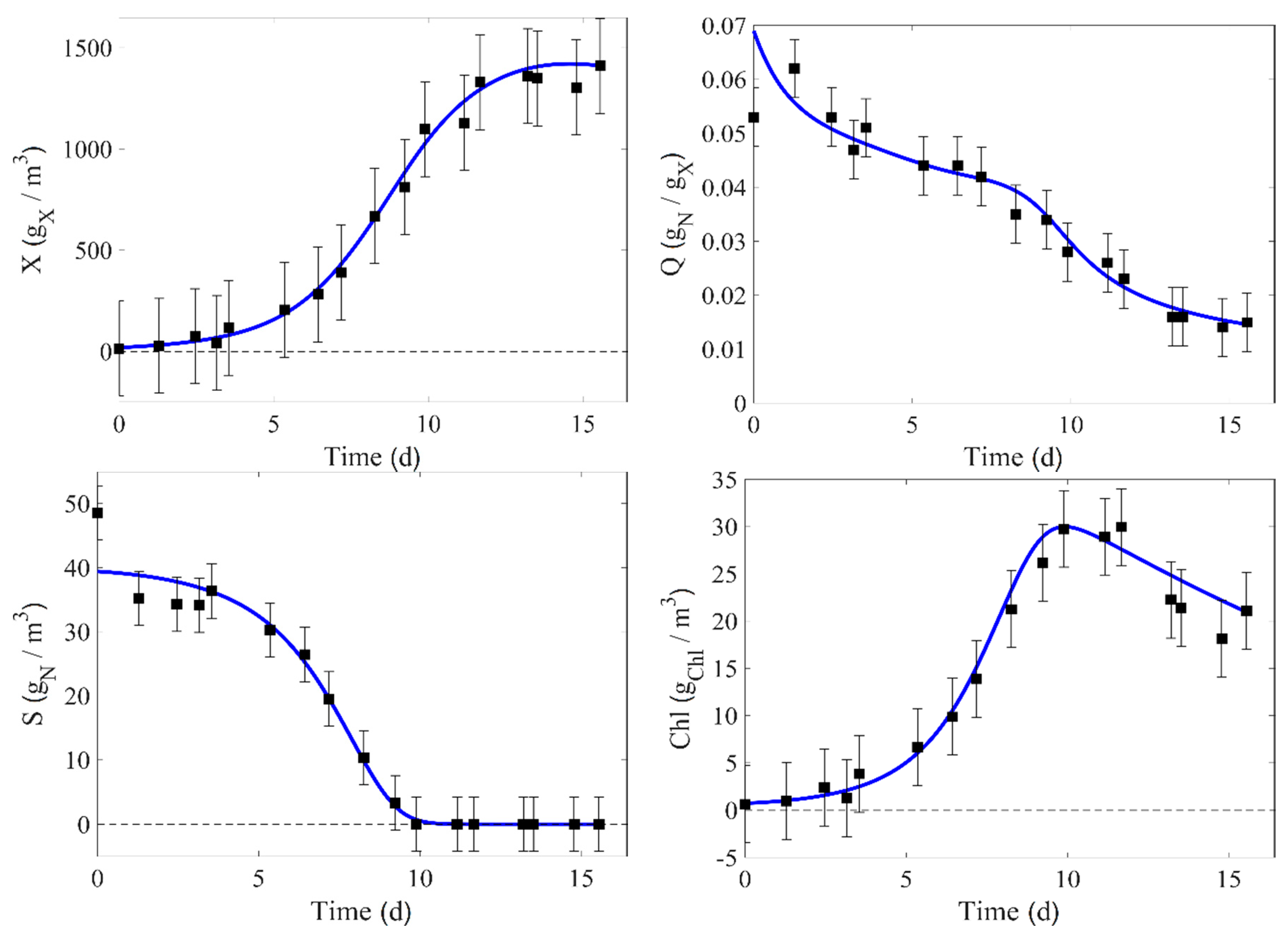
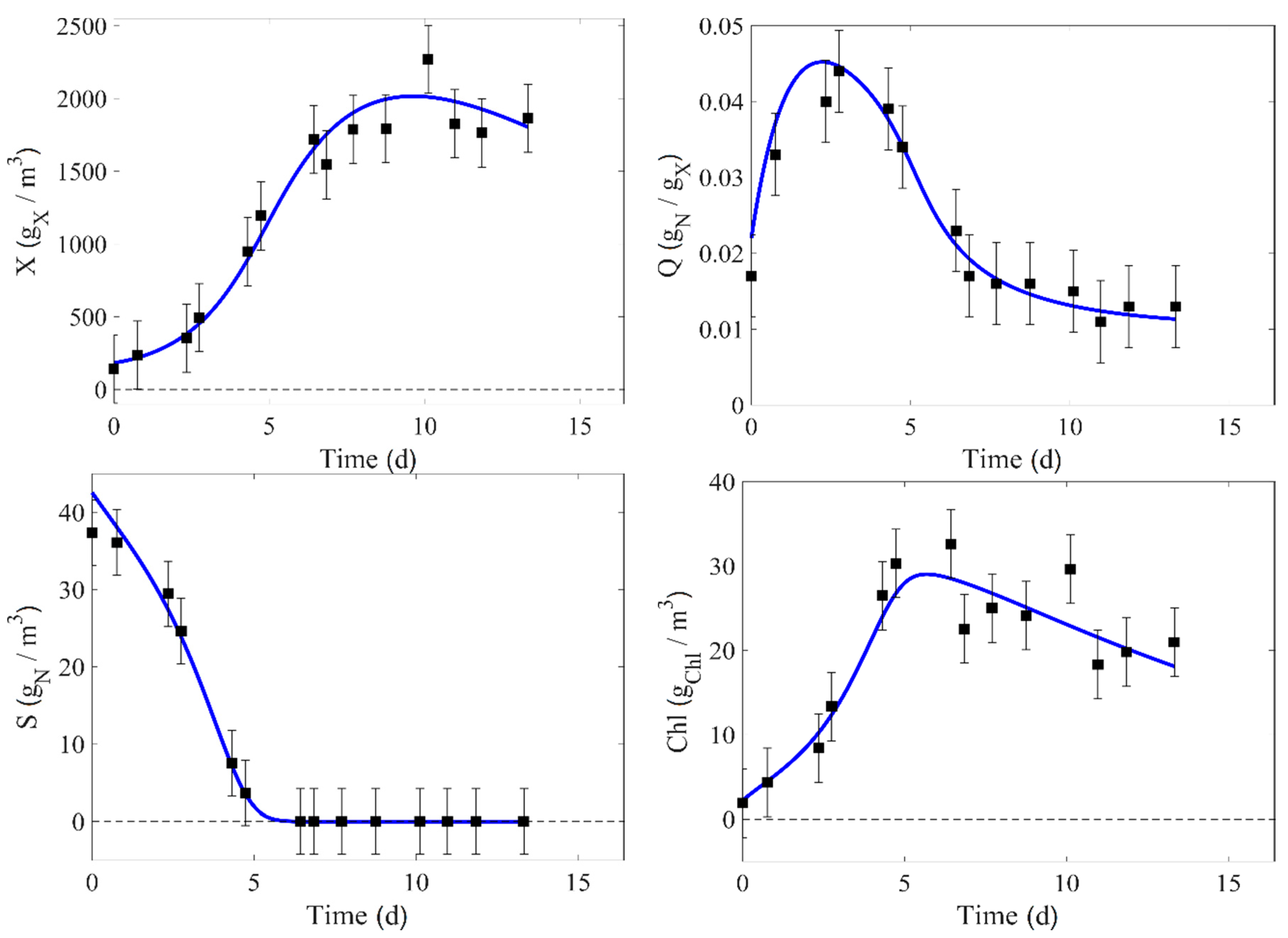
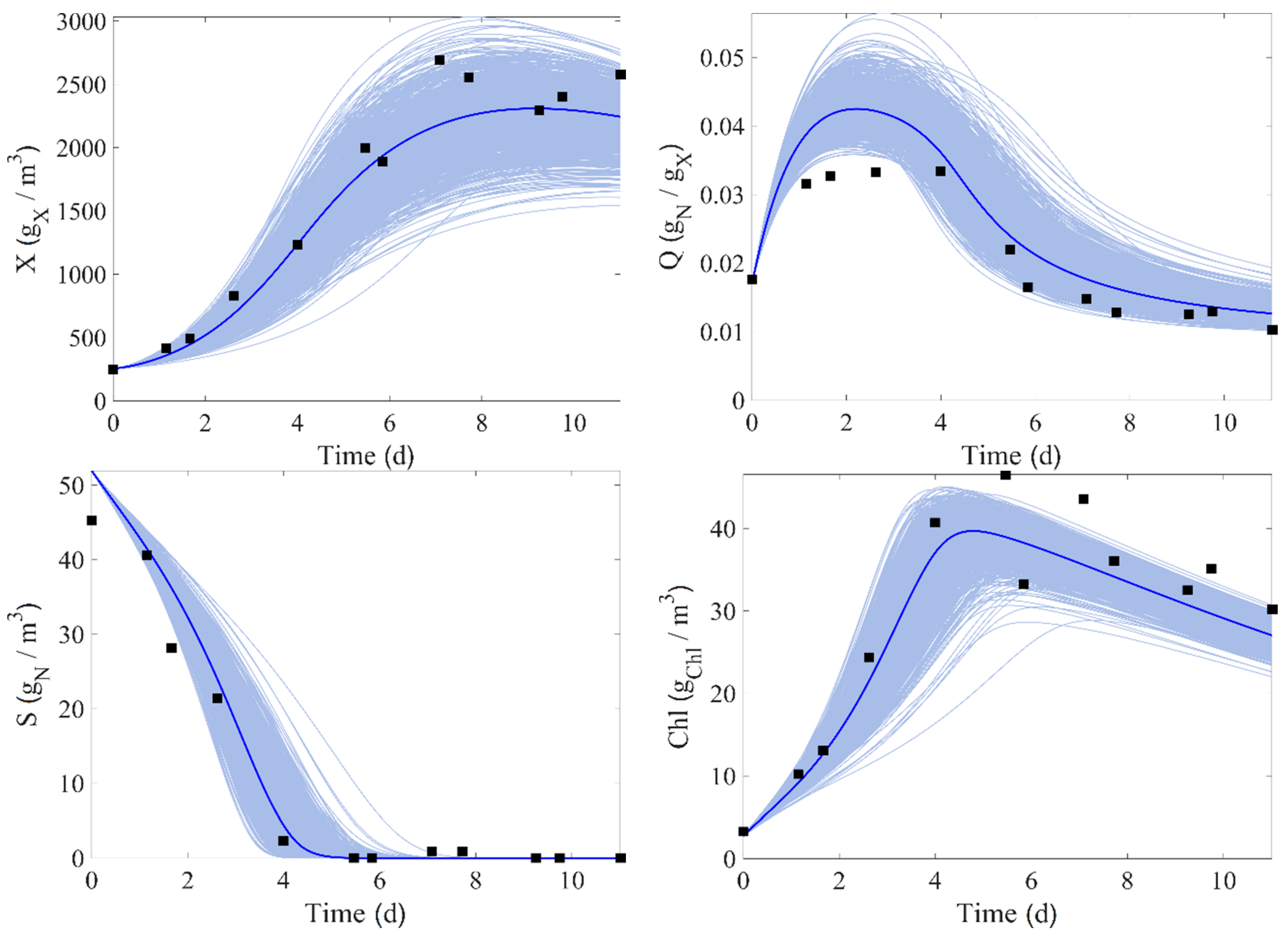
In this work, there is a total of nine experimental runs. Seven of them (runs 1–4, 6–7, and 9) are used for the identification process and direct validation. The experimental data of runs 4 and 9 are compared to the corresponding model prediction in Figure 2 and Figure 3, where the confidence intervals of the measurement at 95% are also displayed (these intervals are estimated from Equation (24)).

An important point is that not only the model parameters are estimated but also the initial conditions of the model state variables. Indeed, these initial values are measured as any other data point and they are therefore uncertain. Nonetheless, they play a critical role in the model integration and a good identification practice is to not completely trust the measured initial conditions as they are corrupted by measurement noise, and thus, to not force the model to exactly start from these points. Hence, initial conditions are estimated as part of the identification procedure. This gives the model more flexibility to fit the datasets. However, the combined identification of the model parameters and initial conditions (of each experiment) leads to a relatively large problem which can be delicate to solve at once. The procedure is therefore subdivided into two steps. It is initially assumed that the errors in the initial conditions are relatively small, and only the model parameters are estimated. In a second step, the model parameters are fixed to their estimated values and the initial conditions are estimated. This two-step process is performed iteratively until there is a convergence—usually achieved in a couple of iterations.

Table 4. Initial conditions for each culture run (Physical units are defined in Table A1).

${\mathit{x}}_0$	$\mathit{X}$	$\mathit{Q}$	$\mathit{S}$	${\mathit{I}}^{*}$
1	8.5	0.019	28.35	104
2	9.8	0.035	28.11	97
3	36.4	0.047	38.08	202
4	14.8	0.053	48.55	209
5	56.3	0.026	36.98	92
6	92.1	0.020	37.19	103
7	249.9	0.019	45.40	261
8	249.0	0.018	45.26	157
9	141.7	0.017	37.38	193

contains the estimated initial conditions.

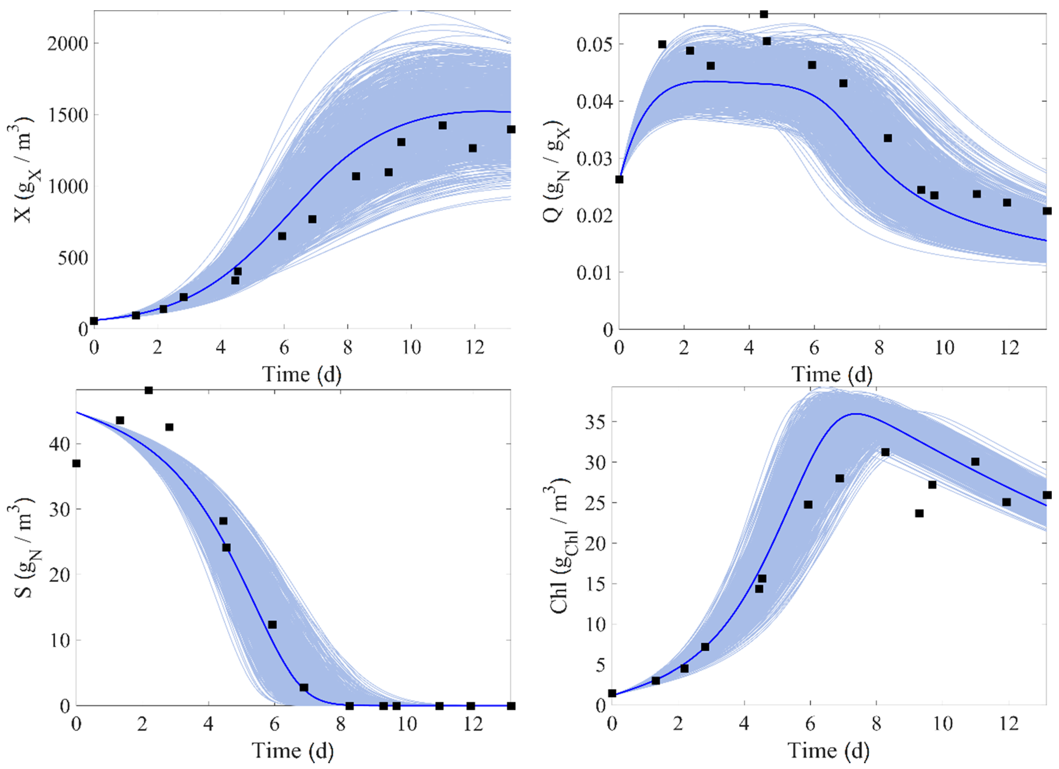
In order to check the model prediction under parameter uncertainty and to compare it in cross-validation, simulations are carried out using a Monte Carlo approach. The parameter set is generated with a Latin Hypercube Sampling (LHS), which can be achieved using the MATLAB^® commands lhsdesign or lhsnorm using the estimated mean and standard deviation of the parameters. For this purpose, runs 5 and 8 are considered and 1000 simulation runs are produced with sampled model parameters (the initial conditions are fixed in this process). Figure 4 and Figure 5 show the results, where the light blue areas represent the range of values taken by each state variables. It can be seen that the trend of the data is well followed by the model, and the experimental data are almost entirely inside the uncertainty intervals.

At this stage, it is interesting to compare our results against the parameters identified in previous works (see

Table 5. Estimated values for model parameters (physical units are defined in Table A1).

Parameter	[26] 1		[29] 2		Current Study 2
	Value	CV (%)	Value	CV (%)	Value	CV (%)
$\overline{\mu }$	1.7	-	1.47	5.9	1.69	7.0
$k_s$	0.0012	-	0.09	39.3	17.69	10.0
$Q_0$	0.050	-	0.011	13.7	0.0104	4.0
$Q_l$	0.25	-	0.099	2.3	0.1172	8.2
$\overline{\rho }$	0.073	-	0.7	15.8	0.0573	6.4
${k_{sI}}^{*}$	1.4	-	0.22	0.1	1.36	17.3
$k_{iI}$	295	-	700	10.5	94.3	14.6
$R$	0.0081	-	0.028	21.8	0.0779	2.1
${\gamma }_{max}$	0.57	-	1.10	3.2	1.158	1.6
$k_{I^{*}}$	63	-	1970	6.0	184	7.7
$a$	16.2	-	17.3	8.8	12.6	37.0
$b$	0.087	-	0.33	10.1	0.72	23.8
$c$	0	-	0.14	19.2	15.1	45.9
$K_g$	-	-	1.22	2.8	10.6	24.5

¹ Parameters for microalgae strain Isochrysis galbana. ² Parameters for microalgae strain Scenedesmus obliquus.

). One of them is [26], where the identification is performed for another strain, Isochrysis galbana and a different version of the model, based on experimental data reported in [45]. Another one is [29], which is based on the model originally reported in [25], with a few simplifications in some physiological variables equations, and experimental data for the same strain, Scenedesmus obliquus cultivated in large cylindrical photobioreactors.

The first study identified the model parameters based on a dataset with a relatively narrow range of conditions corresponding to low biomass concentrations and low photon flux density, as it can be seen in [45]. The second study has achieved the model identification using measurements of biomass, nitrogen quota, and substrate concentration, but chlorophyll was not available at the time, which implies identifiability problems. In this work, our objective was to provide a wider range of operating conditions and to include the measurement of chlorophyll, in an attempt to have a more precise determination of parameters involved in the acclimation and photoinhibition processes.

The reported values of $k_s$ in these previous identification studies are relatively small compared to the actual substrate concentrations, which is not the case in the present study. Considering that it represents the half-saturation coefficient of a Monod law, therefore, the kinetic factor approaches unity, making it irrelevant. The same happens with parameter $K_g$. When comparing the operational values of the optical depth $\lambda$ with $K_g$, the value of $K_g$ is noticeably smaller, which makes the average photon flux density received throughout the reactor almost negligible for most operational conditions, which is probably not realistic. Taking a look at the coefficient $a$, their values are in agreement in the three studies and notably high, which implies that chlorophyll has a strong shading effect in the culture, aside from the biomass darkening effect. The majority of higher impact parameters, like the maximum specific growth rate, $\overline{\mu }$, the maximum nitrogen intake rate, $\overline{\rho }$, the minimum and maximum nitrogen quota, $Q_0$ and $Q_{\mathrm{l}}$, the attenuation coefficient due to chlorophyll, $a$, and the attenuation coefficient due to biomass, $b$, they all have similar values within the same magnitude order.

6. Non-Linear Model Predictive Control (NMPC)

6.1. Background on Model-Based Control of Cultures of Microalgae

The first reported applications of on-line control of microalgae cultures took place in the context of outdoor pounds and used standard feedback controllers to achieve a static optimization criterion [46,47].

Regarding microalgae indoor cultures, several control strategies have been reported, most of them focused on optimizing biomass productivity or following an optimal growth trajectory.

Among them, it can be mentioned a linearizing control approach is performed for the regulation of the biomass density in a closed microalgal photobioreactor [48]. In this application, the photobioreactor system is programmed to operate in a constant biomass density mode, to maintain the culture at the optimal population density and to sustain high biomass production levels. An adaptive control approach can be found in [49], while in [50] a feedback linearization over the light-to-biomass concentration control was proposed, introducing this new variable as the manipulated one. Later, in [51] an optimization of biofuel production through ANN modeling was realized. In [52], a MPC with economic and environmental constraints was implemented. A version of a model-based predictive control relying on an artificial neural network model (ANN) was developed by [22]. In [32], an extremum seeking control was developed based on a block-oriented model for on-line optimization of microalgae productivity, while in [53], the power consumption of the light source was considered within a productivity objective function, and the bioreactor was optimized for manipulating the dilution rate by an extremum seeking control. In [8], optimal values for the dilution rate and the incident photon flux density were provided to maximize the steady-state microalgal surface productivity in a continuous culture.

In practice, the goal is often to maintain the culture conditions in such a way that the productivity of microalgae is close to a maximum. A recent contribution to this subject uses MPC based on a three-state model [52]. In this application, dilution is manipulated for productivity maximization, the influence of light is not modeled, and variation in illumination is conceived as a disturbance to be rejected by the controller.

Most of the control strategies manipulate the dilution rate of the photobioreactor. A different approach can be found in [54] and in [55], where photon flux density is considered for control purposes. Regarding artificial light conditions, the intensity of the incident light can be used to achieve optimal conditions for microalgae growth. Indeed, when light energy is either in excess or too low, the productivity declines. Moreover, to favor an economically competitive production of microalgae, the light energy should be reduced as much as possible, while procuring high efficiency [56].

Nowadays it is well-established that the growth of microalgae cultures depends on two processes: the nutrient uptake and the photoacclimation. In this work, both biological mechanisms are shored up to optimize production. The proposal is based on an MPC scheme that maximizes productivity by means of manipulation of the dilution rate and the light irradiance to the reactor.

6.2. NMPC Setup

The optimization objective is set to maximize the cumulative production of biomass, $P_c$. For such purpose, both inputs are considered as manipulated variables: the dilution rate ($D$) and the light irradiance at the surface ($I_0$). The discrete process model is obtained by integrating the differential equations of the state variables (Equations (2)–(5)) with a sample time $t_{sample}$, while the manipulated variables remain constant along with the sampling interval. At each integration time, the complete set of initial conditions are assumed to be known.

The NMPC considers a prediction horizon of $P$ samples while the objective function (cumulative production) is defined as in [57].

$$J={\displaystyle \sum }_{k=1}^P{P}_c\left(k\right)={\displaystyle \sum }_{k=1}^{P}D\left(k\right)X\left(k\right)$$

(31)

The control horizon is $M$ ($M<P)$, and the control variables are calculated solving the following problem:

$$\underset{D\left(k\right), I_0\left(k\right),k=1, \dots ,M}{\arg \max } J$$

(32)

subject to

$$\dot{\xi }=f\left(\xi , u\right)$$

(33)

$$D^{lower}\le D\left(k\right)\le D^{upper}$$

(34)

$$I_0^{lower}\le I_0\left(k\right)\le I_0^{upper}$$

(35)

Equation (33) stands for the state model described by Equations (2)–(5) and (6)–(13); where $\xi$ and $u$ represent the whole state-vector and the input variables, respectively. The lower and upper bounds on $D$ and $I_0$ considered in Equations (34) and (35) are shown in

Table 6. Manipulated variables bounds.

$D^{lower}$	0.0	$D^{upper}$	1.5
$I_0^{lower}$	0	$I_0^{upper}$	1500

The lower and upper are the boundaries of variables D and I₀.

. Note that the complete set of states is assumed measured at each sampling time.

6.3. NMPC Performance

Figure 6, Figure 7 and Figure 8 depict the time response achieved by the controlled process with $t_{sample}=1 d$, $P=6,$ and $M=3$. These settings provide a good trade-off between productivity and computing time. The optimal photon flux density is established at a level which favors the biomass growth while avoiding inhibitory effects. On the other hand, the dilution rate is relatively low, which allows a sufficient nutrient inlet to maintain the growth rate but alleviates the risk of wash-out. To perform the optimization, the MATLAB^® solver fmincon is used. At each iteration, the objective function is computed by integration of the dynamic model over the prediction horizon. The previous time solution is used as an initial guess for the manipulated variables.

These figures show that the best strategy to enhance productivity is to maximize biomass growth during the first days. The controller initially increases the biomass concentration inside the photobioreactor up to a plateau where the photon flux density and the dilution rate vary more slightly, with changes linked to the adaptation of the culture, mainly due to the chlorophyll concentration. As observed in Figure 8, the profiles of the manipulated variables do not exhibit sudden changes or sustained switches, which is desirable for later implementation. As the controller approaches the end of the production cycle, the prediction and control horizon are reduced. This implies that the controller tries to increase the instantaneous productivity without taking care of the future—beyond the end of batch at 20 days—biomass production any longer. This is not necessarily a desired behavior, but it illustrates well the possible exploitation of the model and the NMPC.

Having a complete phenomenological model and using both variables for control allows avoiding microalgae photoinhibition whose occurrence would drastically diminish biomass growth. This optimization approach was possible due to the detailed model reported in [26], based on a Droop representation supplemented by appropriate kinetics accounting for photoacclimation, photoinhibition, as well as light absorption and diffusion.

An important characteristic of microalgae cultures is the darkening effect that happens with increasing concentration of biomass or chlorophyll. This, coupled with the physiological response to the photon flux density—adaptation of the chlorophyll concentration—makes the optimal light intensity vary at every moment. Microalgae in general tend to have a higher concentration of chlorophyll when they are exposed to a lower light intensity, but as the light intensity increases, the concentration of chlorophyll decreases, and eventually, the growth can even be stopped. In particular, the species of microalgae used, Scenedesmus obliquus, is used to environments with low light intensity. Although the intensity received by the crop surface is relatively high, the controller manages the conditions so that the average photon flux density, $\overline{I}$, through the crop is much lower, close to the optimum photon flux density, $I_{opt}$, which is mathematically required by the culture so as to achieve the best performance (Figure 7).

7. Conclusions

Based on datasets collected from cultures of the microalgae Scenedesmus obliquus in laboratory-scale photo-bioreactors, a dynamic model could be successfully identified. This model is highly nonlinear, and includes a description of the photo-acclimation and photo-inhibition phenomena exhibit by microalgae. A wide range of operational conditions has been explored, including incident light, biomass, and substrate concentrations. The overall identification and further validation of the model were shown to be satisfactory. This model allows studying the behavior and response of the system, especially to characterize the inhibitory effect of light and the impact of the dilution rate, both critical for the photobioreactor performance.

As a prospective application, a NMPC control strategy manipulating both inputs—dilution rate and photon flux density—was then explored. The microalgae biomass production can be significantly enhanced by the correct manipulation of these control variables; this control strategy constitutes a natural and effective approach to the optimization problem.