Optimal Speed Control for a Semi-Autogenous Mill Based on Discrete Element Method

School of Automation, Central South University, Changsha 410083, China
*
Author to whom correspondence should be addressed.
Processes 2020, 8(2), 233; https://0-doi-org.brum.beds.ac.uk/10.3390/pr8020233
Submission received: 9 December 2019
/
Revised: 12 February 2020
/
Accepted: 12 February 2020
/
Published: 18 February 2020
(This article belongs to the Special Issue Process Optimization and Control)
Abstract
:The rotation speed of a mill is an important factor related to its operation and grinding efficiency. Analysis and regulation of the optimal speed under different working conditions can effectively reduce energy loss, improve productivity, and extend the service life of the equipment. However, the relationship between the optimal speed and different operating parameters has not received much attention. In this study, the relationship between the optimal speed and particle size and number was investigated using discrete element method (DEM). An improved exponential approaching law sliding mode control method is proposed to track the optimal speed of the mill. Firstly, a simulation was carried out to investigate the relationship between the optimal speed and different operating parameters under cross-over testing. The model of the relationships between the optimal rotation speed and the size and number of particles was established based on the response surface method. An improved sliding mode control using exponential approaching law is proposed to track the optimal speed, and simulation results show it can improve the stability and speed of sliding mode control near the sliding surface.
1. Introduction
In modern mineral processing, semi-autogenous (SAG) mills are important grinding equipment. A SAG mill has the advantages of high operation rate, large output, and large crushing ratio, which makes SAG mills have the characteristics of short process time, low management cost, and suitability for large-scale production compared to other mills. Therefore, SAG mills are favored by large mines and are becoming more and more widely used in the mineral processing industry [1,2]. A SAG mill has low speed and heavy load, which cause the energy consumption of grinding operation to be very high. It accounts for a large proportion of the electrical consumption across the plant [3].
The rotation speed is an important factor related to the operation and grinding efficiency of the mill. Under the traditional operating procedures, constant speed grinding is usually adopted, which consumes a lot of energy, has a great impact on the equipment, and has a high amount of returned sand, and therefore the output of the process is restricted. However, with the gradual emphasis on energy conservation and emission reduction, higher requirements have been put forward for process stability, grinding optimization, equipment stability, and service life. Therefore, an effective and efficient approach for optimization and control of the SAG mill speed is of great economic significance.
In the actual mineral processing, the SAG mill operates at a constant speed after acceleration from standstill, which may not be the optimal speed [4]. Mill rotational speed may be variable, and in some cases increasing speed can increase grinding capacity [5]. In a SAG mill, operation with variable speed presents significant advantages in terms of productivity and efficiency [6]. However, as the speed increases, the load is partially lifted in the SAG mill [7]. At 100% operating speed, the expected torque with 30% load and 20% of balls reaches an overload trip in the SAG mill [8]. When the mill speed is constantly changing, liners’ and lifters’ wear is affected as operators change the operating speed to maintain the power draw, which causes the liners’ and lifters’ lifting capacity to be reduced [9]. When the SAG mill speed is higher, the particles stay in the mill for short periods of time, and the speed enhances major impacts between particles, which can cause damage to the liners [10]. The ability to make the mill speed reach the optimal speed is critical when it comes to optimizing mill efficiency and overall productivity [11], so the mill optimal speed ensures the highest possible grind for the given ore target [12]. However, adjusting the mill speed to the optimal state presents a very challenging problem. In a SAG mill, the speed control system is a nonlinear and strongly coupled multivariable system. The proportional integral (PI) vector control method is used in the mill control system [13]. The PI vector control method cannot meet the requirements of high-performance control when the mill speed control system is subjected to external disturbance. Hence, many modern control methods, such as neural network, fuzzy control, and sliding mode variable structure control (SMC), have been applied to the mill speed control system in order to improve the stability of the devices at optimal speed [14].
To obtain the optimal rotation speed of the SAG mill, we must calculate the motion of the particles and balls accurately. Discrete element method (DEM), which can provide dynamic information of individual particles and handle multiple particle contacts [15], has become an important tool for conducting research on large scale equipment in mineral processing [16]. This method has been used extensively to improve the efficiency of the comminution devices [17]. Mishra and Rajamani [18] first applied DEM to the simulations of the charge motion in a 2D ball mill. Cleary and Sawley [19] simulated a 3D ball milling as a part of the DEM modeling of the industrial granular flows. Cleary [20,21] is the pioneer in studying semi-autogenous grinding mills using DEM. Weerasekara et al. analyzed the effects of mill size and charged particle size on the energy in grinding using DEM modeling and drew many interesting conclusions [22]. Studying tumbling mills (e.g., ball mills and SAG mills) using DEM has attracted many researchers’ interests as reviewed by Weerasekara et al. [23] in the fields of charge motion and power draw, effects of grinding media shape, breakage of particles, and so on.
The pioneer researchers and scholars have studied the performance of SAG mills by numerical simulation or theoretical research, but the relationship between the optimal speed and different operating parameters is rarely studied. In this study, the relationship between the optimal speed and the size and number of particles in the SAG mill was mainly investigated based on discrete element method. For optimal speed control, an improved sliding mode control of the exponential approaching law is proposed to improve the stability and rapidity of sliding mode control near the sliding surface compared to the traditional exponential approaching law.
The rest of the paper is organized as follows: the working principle of the SAG mill is briefly described, and the effect of the falling point of the grinding medium in the drum on the speed of the mill is analyzed in Section 2. Modeling of the semi-autogenous mill based on discrete element method is outlined in Section 3. In Section 4, sliding mode control of the SAG mill motor is presented. In Section 5, conclusions are drawn.
2. Working Principle of SAG Mill and Energy Analysis
2.1. Working Principle of SAG Mill
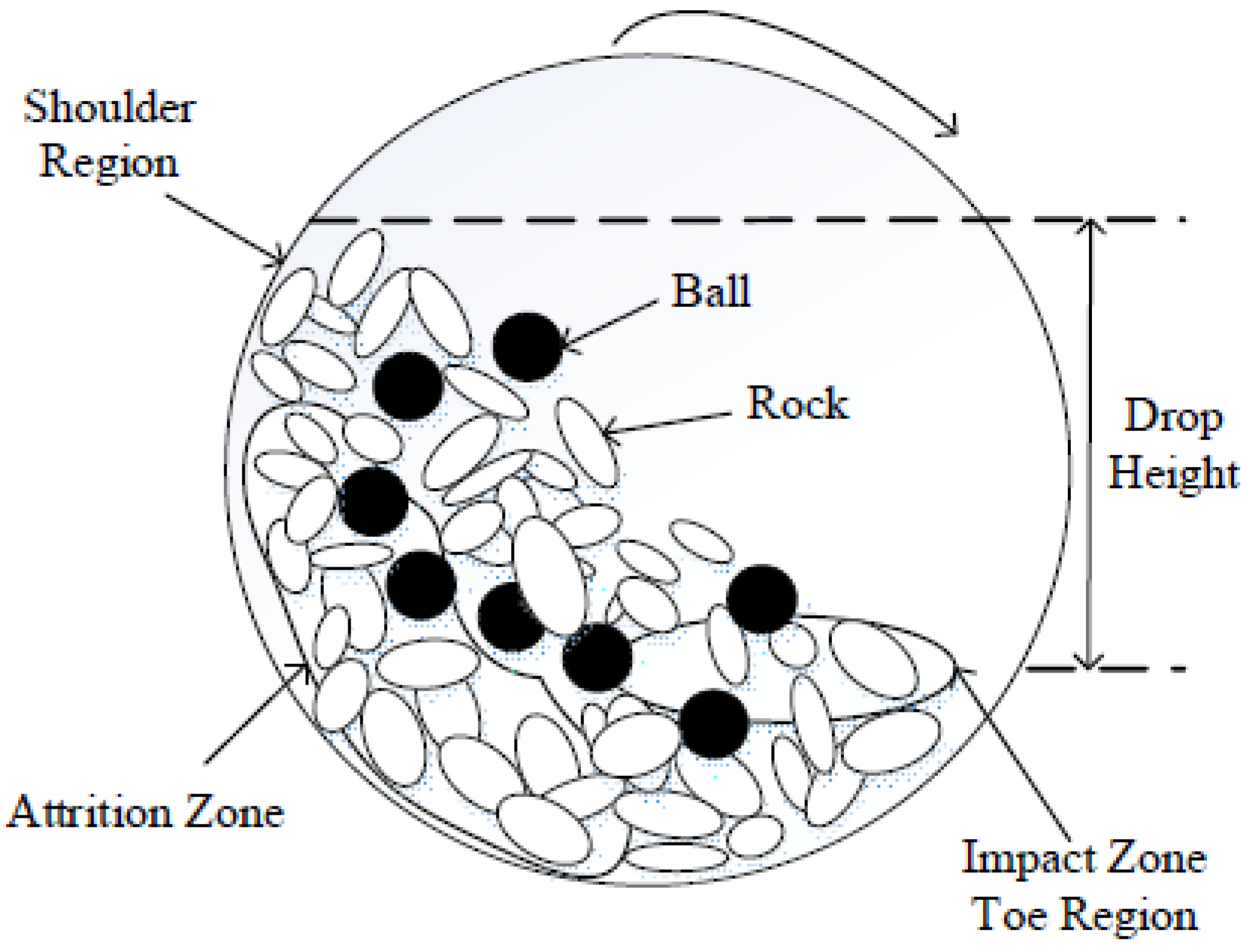
The main components of a SAG mill are transmission structure, roller, slow drive, and feeding and discharging device. The working principle of a SAG mill is as follows: the main motor drives the roller to rotate through the transmission device, and the grinding medium performs the rotary ascending motion under the action of the lifting strip and the friction force between the materials and the centrifugal force. After reaching a certain height, a part of the material and the steel balls with high speed are separated from the roller to make a falling motion, and the material is broken by the impact force generated during the falling process. Another part with a lower speed is separated along with the roller. The roller makes a sloping motion, which causes collision and friction between the material, the steel ball, and the lining plate. Thus, the material is ground and peeled off. The schematic diagram of the working principle of a SAG mill is shown in Figure 1. The shoulder area inside the drum represents the area where the steel balls and the material are separated from the barrel to start throwing after they are lifted to a certain height due to rotation. The toe region refers to the ore toe area, where the grinding medium falls on the ore below to produce impact when it is dropped. The attrition zone refers to the kidney-shaped peristaltic zone, in which the movement of ore is very slow and there is little collision. It can be regarded as “peristalsis”, which has little impact on the grinding effect.
2.2. Energy Analysis of the Grinding Medium
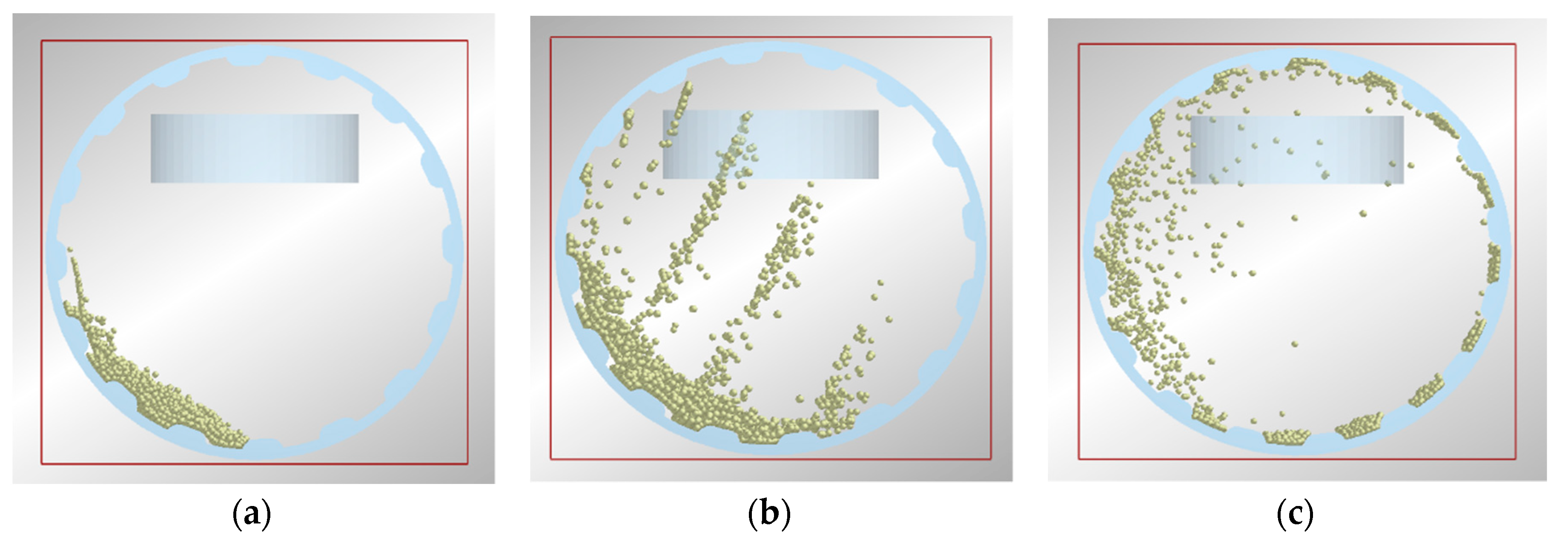
There are roughly three types of grinding balls: cascading type, throwing type, and centrifugal type, as shown in Figure 2. The cascading type grinding ball has little impact on the material, and the grinding efficiency is low. Under the centrifugal motion of the grinding balls, the grinding process is basically stagnant without any grinding effect; the grinding efficiency can be improved only when the grinding balls are thrown as shown in Figure 2b.
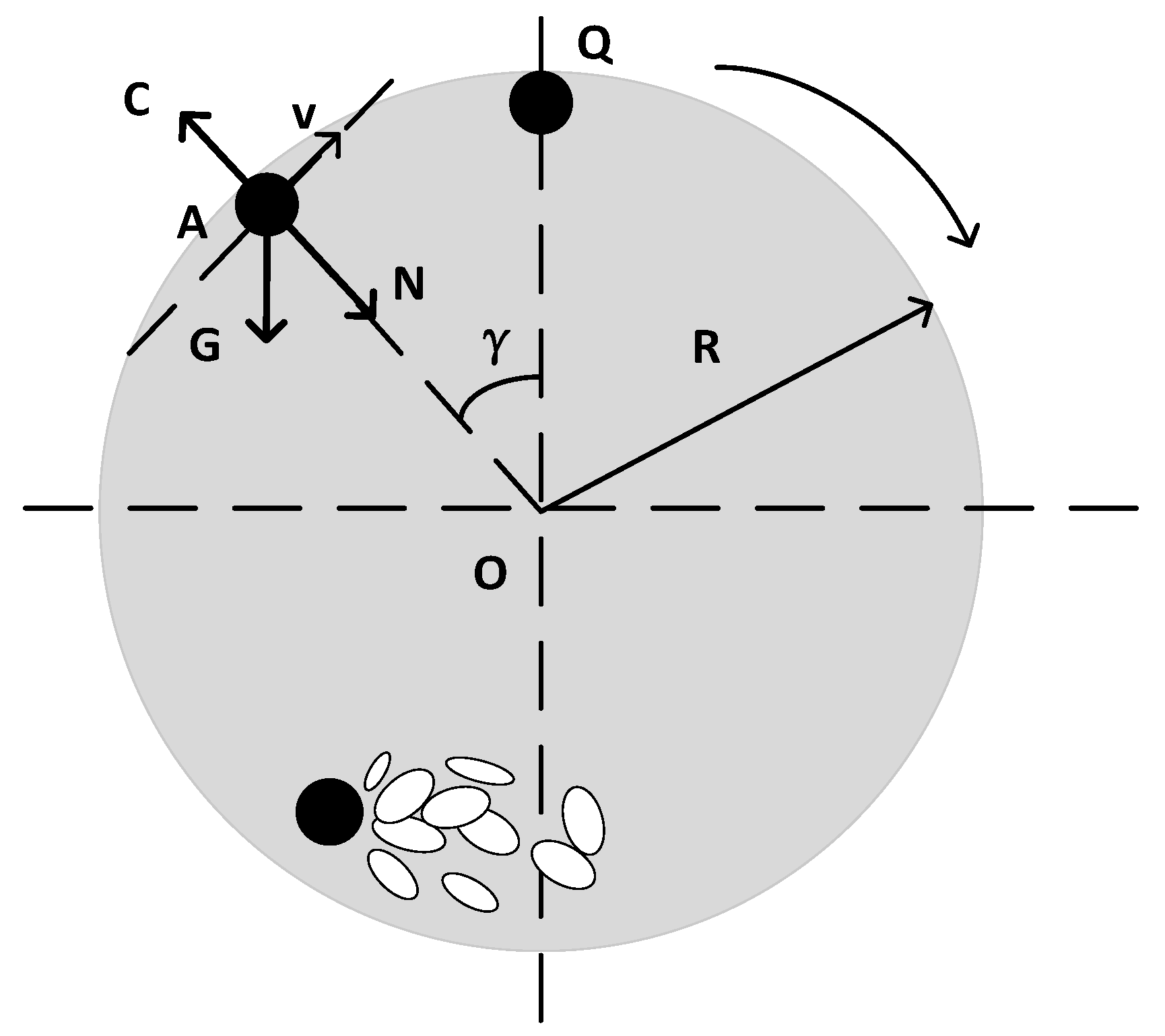
Figure 3 shows the grinding ball is in throwing motion. Point A is the position where the grinding ball is separated from the drum wall of the roller. The linear velocity of the thrown ball at point A is denoted as v. The angle between OA and the vertical direction is denoted by γ. When the rotation speed of the SAG mill increases, the value of γ decreases. When the mill rotation speed is increased so that γ is zero, the grinding ball is in centrifugal motion, and the critical point is denoted by Q as shown in Figure 3. Thus, when the grinding ball is in throwing motion at point A in the shoulder region, γ is greater than zero, and meanwhile it must not be greater than 90°. According to [24], it is assumed that there is no relative sliding between the drum wall and the grinding ball, and meanwhile the volume of the ball and all friction forces are ignored, and the kinematic equation at point A is
where N is the reaction force of the drum wall against the grinding ball; C is the centrifugal force of the grinding ball when it moves with the SAG mill in a circle; and G is the gravity of the grinding ball.
When the grinding ball leaves point A, it has N = 0, and the centrifugal force C of the grinding ball is mv2/R, where m is the mass of the ball and R is the radius of the roller. According to Equation (1), it has
The trajectory of the ball after being thrown from point A is shown in Figure 4. When a coordinate axis is built with O as the center, the coordinate of point A is then (−Rsinα, Rcosα), where α is the angle denoted in Figure 4. In order to study the trajectory of the ball more simply, a coordinate axis is built with A as the center. Then, it has
where x and y are the horizontal coordinate position and the vertical coordinate position, respectively, after the ball is separated from point A. That is, (x, y) is a point on the trajectory by taking point A as the center.
It is noted that under a certain rotation speed of the mill, α is equal to γ and is a constant. Then, from Equation (2) it has cosα = v2/(gR).
Meanwhile, according to the parabolic principle, the trajectory equation of the ball is
Suppose B is the falling point of the dropped grinding ball from separation point A. The falling angle is β, and the coordinates of point B can be obtained by combining equation cosα = v2/(gR) and Equations (3) and (4),
where, xB is the horizontal coordinate position and yB is the vertical coordinate position of the grinding ball at point B.
When the grinding ball is dropped from the highest point D on the trajectory to the falling point B as shown in Figure 4, the falling height H of the grinding ball has the maximum value. Equation (6) is then obtained to solve the falling height H by first order derivation of Equation (4),
Therefore, let the above equation be equal to zero. xD and yD can be obtained by combining equation cosα = v2/(gR) and Equation (4),
where xD is the horizontal coordinate position and yD is the vertical coordinate position after the grinding ball is separated from point A to the highest throwing position point D.
Thus, the falling height of the grinding ball can be obtained by combining Equations (5) and (7). It has
When the grinding ball is dropped from the highest throwing position to the falling point B, because the grinding ball is falling approximately freely, the throwing motion of the grinding ball is decomposed into the approximate free fall movement in the vertical direction and the uniform motion in the horizontal direction. It can be derived from equation cosα = v2/(gR) and Equation (8) to get
Then, the resultant velocity of point B can be expressed as follows:
If the mass of the grinding ball is m, its kinetic energy at the falling point B can be derived from Equations (10) and (11) to get
From Equation (12), the kinetic energy of the ball falling is related to α and the drop velocity v, which in turn depends on the relationship of speed rate (namely speed) and the filling rate. Therefore, changing the falling point of the grinding ball by adjusting speed and filling rate, the purpose of which is to increase the number of grinding balls in the dropping area, can cause more grinding medium to drop to achieve greater impact on ore and better grinding effect. When the number of particles in the throwing movement reaches the maximum, the best grinding effect is achieved. It can be considered that the mill speed at this time is the optimal speed.
3. Optimal Speed Model for SAG Mill Based on Discrete Element Method
DEM has been used by many scholars to study the grinding mechanism and grinding performance of ball mills and SAG mills under different conditions. In this section, a simulation was carried out by using DEM software to investigate the variation of speed with number and size of particles. Two materials were considered, including practice material and steel balls, for DEM simulation. The parameters and conditions for simulation are shown in Table 1.
3.1. Simulation Experiment Design and Simulation Procedure
Based on the detailed analysis of the grinding process of the SAG mill, a three-dimensional simplified model of the SAG mill roller with the specification of Φ 6 × 4 m was established by using software UGNX8.0. The model was then imported into the discrete element software EDEM, and a particle factory was established approaching the roof inside of the roller, and particle movement was simulated in the roller of the SAG mill. Different parameter combinations were used for simulation calculation in this experiment. The parameters were number and size of particles, which were used to reflect the influence of the filling rate of the mill on the optimal speed. The best filling rate of the mill is generally 30%–40%. The range of the number of particles was 5000 to 15,000, with a step of 500 as shown in Table 2. The range of particle sizes was 50 to 100 mm, with a step of 5 mm. The highest filling rate is set approximately at 50%. Speed rate refers to the ratio of the speed of the mill to the critical speed, where the critical speed is . In practice, the speed rate of the SAG mill is generally 65% to 80%. Therefore, in the experiment, the speed was set to vary in 50% and 90% of the critical speed (1.28–1.64 rad/s) for the cross-over test as shown in Table 2.
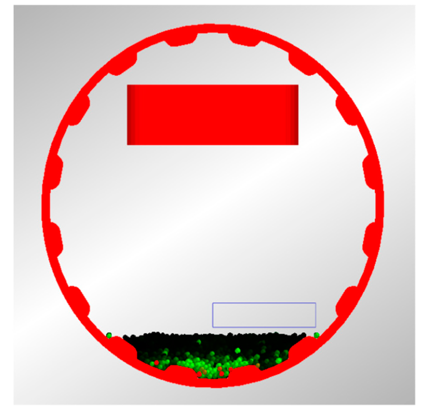
The dropping area was set by using the grid bin group function in the software EDEM and was positioned inside the roller as shown in Figure 5. As the dropping motion of the steel ball is the main role of the SAG mill to grind the ore, when the milling process is stable, the more particles (represented by NZ) fall into the zone, the better the grinding effect is. The number of particles and particle size were set for the cross-over test. Within the parameter ranges, a simulation was carried out with the step of 0.005rad/s for the speed as shown in Table 2. Then, the speed corresponding to the maximum value NZ under each combination of different values of the parameters was approximately the optimal speed. The relationship between the optimal speed and the size and number of particles was then obtained by using the response surface method as , as detailed in the next section.
3.2. Experiment Results and Optimal Speed Modeling
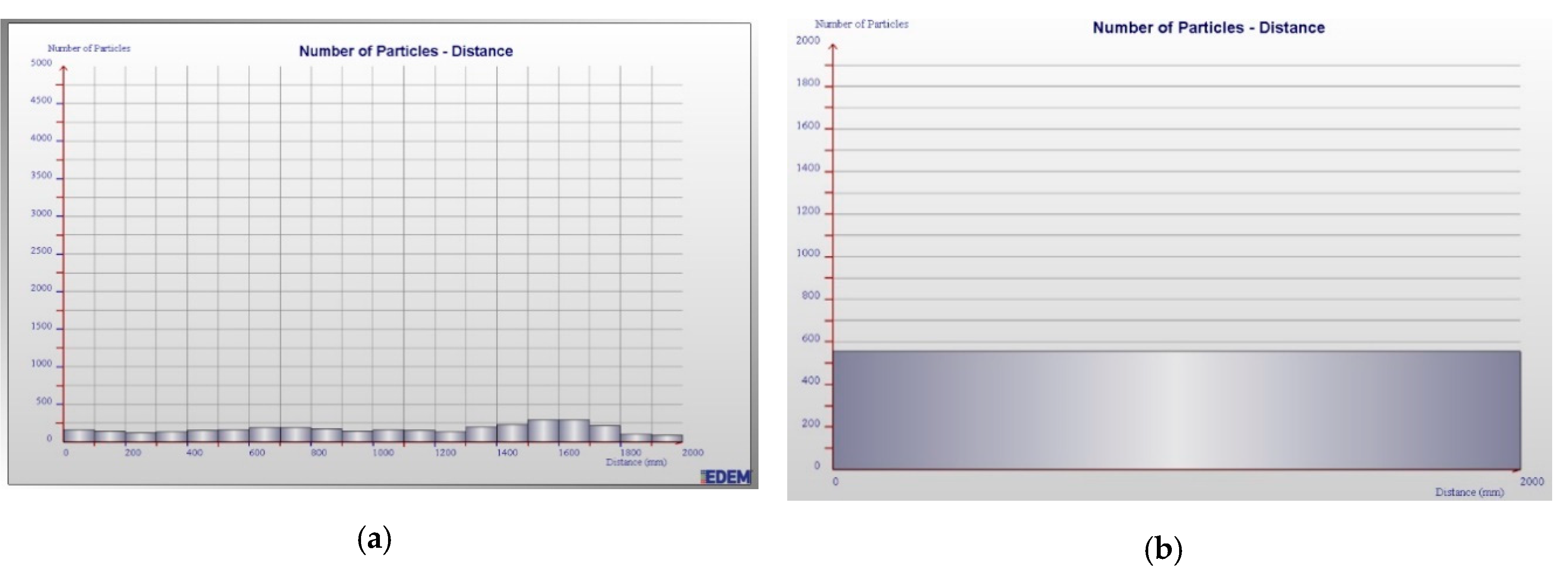
A large number of simulation experiments were carried out. The number of particles falling into the dropping area were recorded under a combination of different values of the parameters. In each run of simulation, the dropping area was divided into several small areas according to the abscissa, and the number of particles dropped in each small area was calculated to analyze the dropping movement of particles in the drum. The results with values of each parameter are shown in Figure 6. Figure 6a shows the number of particles dropped in each small area. Figure 6b shows the number of particles dropped in the whole dropping area, which is the final recorded value of NZ.
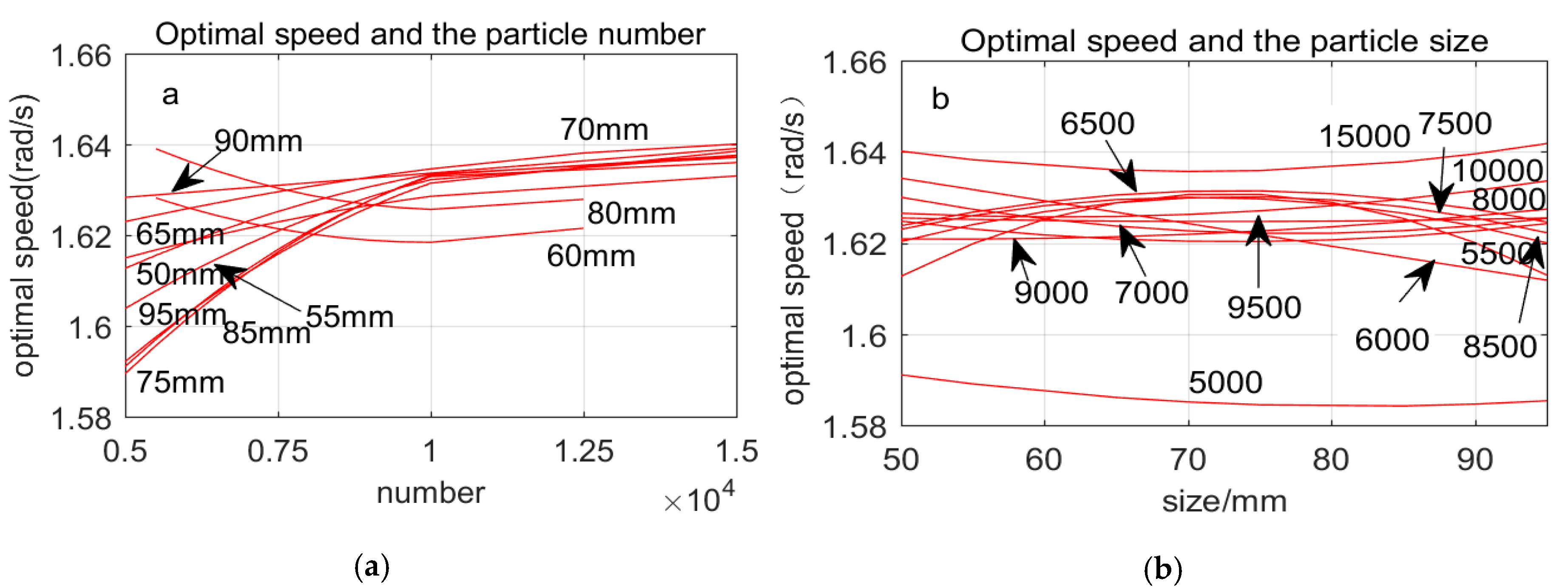
Linear fitting was carried out for the data processing of Figure 7a,b to observe the general trend relationships between the optimal rotation speed and the size and number of particles. Under the same particle size but different number of particles, it corresponds to an optimal rotation speed. The relationship between the optimal rotation speed and the number of particles under different particle sizes is shown in Figure 7a, while the relationship between the optimal speed and different particle sizes under different numbers of particles is shown in Figure 7b.
As shown in Figure 7a, when the particle size is constant, the number of particles increases, and the value of the optimal speed generally shows an upward trend. When the number of particles increases to a certain value, the value of the optimal speed increases slowly. Figure 7b shows that when the number of particles increases, rotation speed generally shows a slow upward trend, but the upward trend is not obvious and is sometimes even downward. This shows that in the case of particle size being too large, increasing the rotation speed of the SAG mill does not necessarily improve the grinding effect.
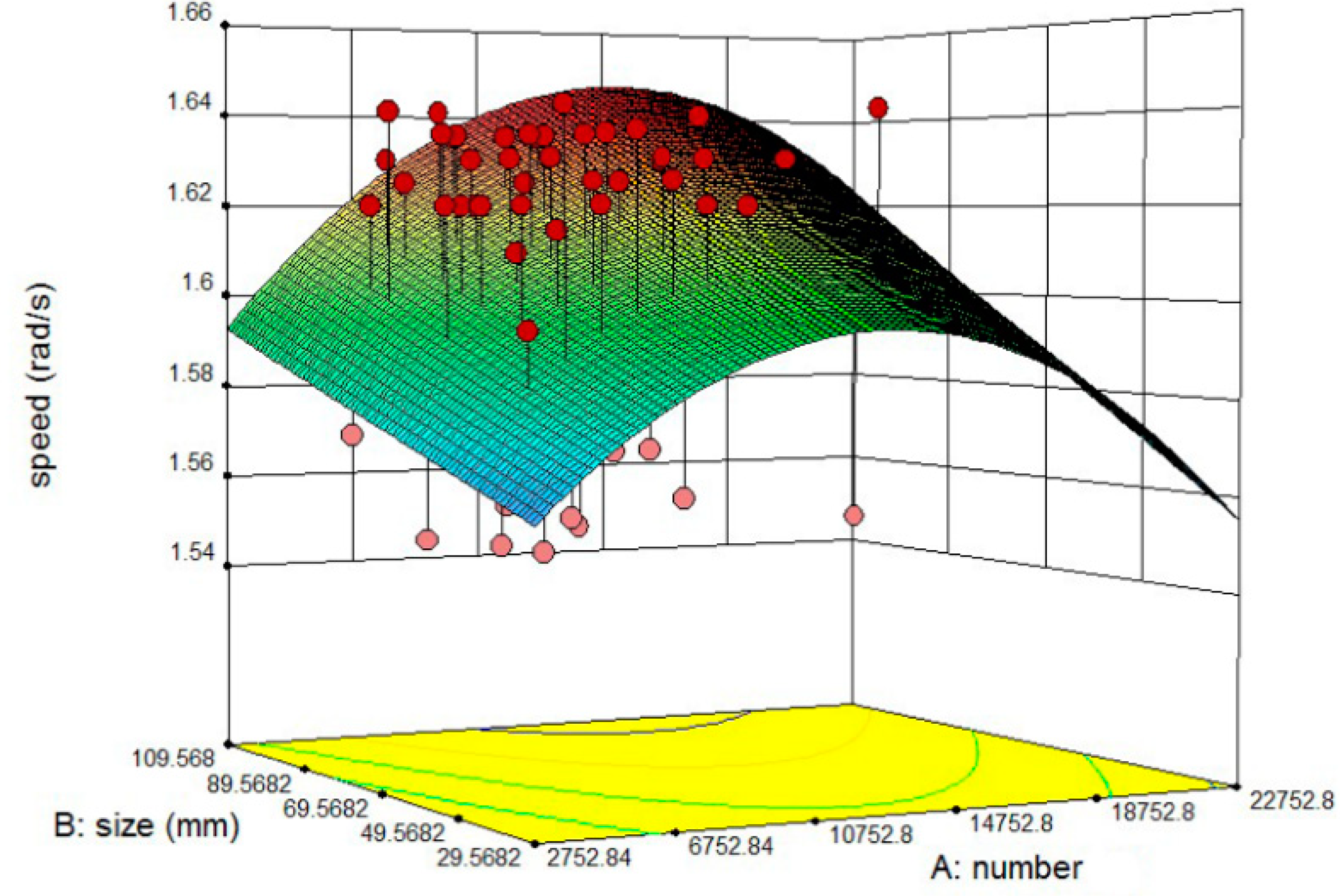
The response surface analysis method was used to analyze the results. The response surface method (RSM) is a statistical method that uses a multiple quadratic regression equation to fit the correlation between the factors and the response values and therefore to seek the optimal process parameters through the analysis of the regression equation. It is suitable for solving multivariable problems.
The correlation was fit by using the corresponding data generated when the particle size was 50, 60, 65, 70, 80, 85, and 90 mm, respectively. In the process of response surface analysis, it can be found that the particle size and the number of particles are two independent variables in the model and influence each other, so there is a large error when the linear model for analysis is adopted. When the order of the model reaches three or higher, there are too many decimal places, which has little impact on the results. Therefore, the quadratic model was used for modeling. The model of the optimal speed is finally obtained as follows:
In order to test the significance of the model, analysis of variance is shown in Table 3, where A represents particle size, and B represents number of particles.
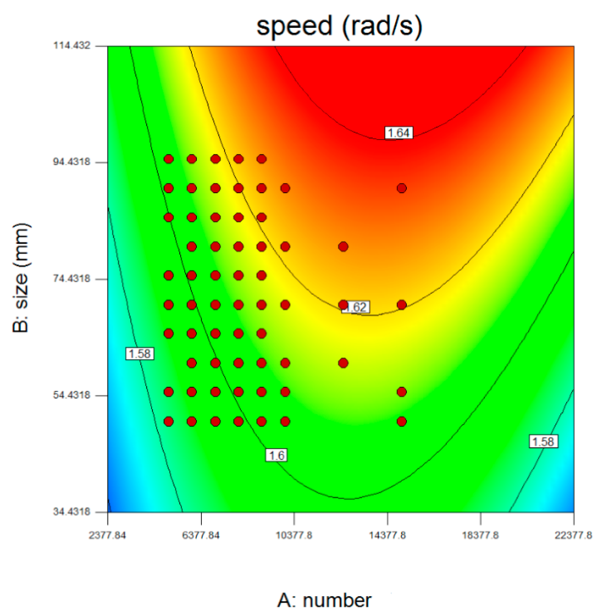
Table 3 shows that the value of “p > F” is 0.0470 < 0.05, which indicates that the quadratic model established has significant performance. The value of primary term “p > F” is B > A, which indicates that the influence of the number of particles on the optimal speed of the SAG mill is greater than that of particle size.
The 3D surface diagram of the response surface is shown in Figure 8. Figure 9 shows the contour map of the response surface. When the particle sizes are 55, 75, and 95 mm, it can be found that the deviation of speed by using the response surface is small. The result can prove the correctness of the response surface to some extent.
4. Sliding Mode Control of the SAG Mill Motor
After the optimal speed under different conditions was determined, the motor needed to be controlled to track the optimal speed. Therefore, the motor model is presented, and a sliding mode control law is proposed to regulate the motor speed.
4.1. Motor Model of SAG Mill
When the gear ratio between the motor pinion and the big gear on the outside of the roller is known, the rotation speed of the mill roller can be controlled by controlling the rotation of the motor. In the actual production, the SAG mill is mostly connected with the AC power grid. A synchronous motor or an asynchronous motor can be used for AC speed regulation. For large capacity AC motor speed regulation, a synchronous motor is usually used. The mathematical model of a synchronous motor [25] can be expressed as
where s represents the stator and d is the rotor; is the vertical axis synchronous inductance coefficient; is the horizontal axis synchronous inductance coefficient; is the mutual inductance when the axis of the stator winding and the excitation winding coincides in the same direction; is the mutual inductance when the axis of the stator winding and the horizontal axis damping winding coincides in the same direction; is the mutual inductance when the axis of the stator winding and the vertical axis damping winding coincides in the same direction; is the excitation current; and are the d-axis and q-axis flux, respectively; and are the d-axis and q-axis equivalent currents, res.ectively; is the electromagnetic torque; is the load torque; P is the number of poles; and J is the total moment of inertia, kg·m2.
For surface mount permanent magnet synchronous motor (SMPMSM), suppose . The torque equation can be expressed as
4.2. Improved Exponential Approaching Law
Many factors affect the optimal speed of the SAG mill. They also affect each other and interfere with each other. Sliding mode control is a special kind of nonlinear control, and it is completely robust to its own parameter perturbations and external disturbances. Therefore, the sliding mode control is adopted to regulate the motor speed of the SAG mill.
According to the experimental design and modeling, particle number and particle size need to be considered in the sliding mode control. The corresponding optimal speed multiplied by the gear ratio is the target speed of the motor. Taking and the gear ratio of the large and small gears as n, the target speed of the motor is
The state variable of the system is
where w0 is the target rotational speed of the motor, and w is the actual speed of the motor.
Then, the expression is derived through Equations (18), (19), and (21).
By defining , the system state space equation is rewritten as
One order sliding surface is selected, and denoting the sliding surface of the system as s,
In order to improve the stability of the system approaching motion, the exponential approaching law is chosen to weaken the chattering of sliding mode control [26]. The exponential approaching law can be written as
where is the isokinetic approach term and is the exponential approach term. When the moving point is far away from the switching surface, the larger the value of k is, the faster the approaching speed is. As the approach point approaches, the switching surface and s decreases and the approaching speed of the law begins to decrease. When the moving point is very close to the switching surface, the approaching speed approaches zero, which is not conducive to the reachability of the sliding mode motion, and the sliding mode motion cannot approach the sliding mode surface quickly. At this time the isokinetic approach term responds. When s approaches zero, the approaching velocity becomes ε, which makes the moving point reach the switching surface in a limited time.
In order to change the approaching speed of the law, the values of k and ε of exponential and isokinetic approaching terms can be adjusted. Generally speaking, if the value of ε is smaller and the value of k is larger, the moving point approaches faster and there is less chattering.
The stability of sliding mode motion should be ensured in sliding model control, choosing the Lyapunov function v(x) = 1/2*s2 [25] as
As , it can be known that
Considering the problem of slow approaching speed of the traditional exponential approaching law, the exponential approaching law sliding mode control is improved here. Introducing the squared term e2 of the error into Equation (25), it yields an improved exponential approaching law as shown in Equation (28):
where e is the error between the system input and output.
In the improved exponential approaching law, when the moving point is far away from the switching surface, since e is large, e2 is also larger. At this time, not only does the constant velocity approaching term k act, but the moving point is also at constant speed. When the moving point reaches the vicinity of the switching surface, the exponential approaching term acts at this time as e2 approaches zero, making the moving point approach the switching surface quickly.
According to Equations (24) and (28), the compensations to the controller can be expressed as
Compared with the traditional exponential approaching law, the improved approaching law can improve the approaching speed of moving points and reduce chattering. Stability of the sliding mode control can be analyzed by using the Lyapunov function v(x) = 1/2*s2 as
As and , it can be known that the stability condition is satisfied.
4.3. Simulation Results
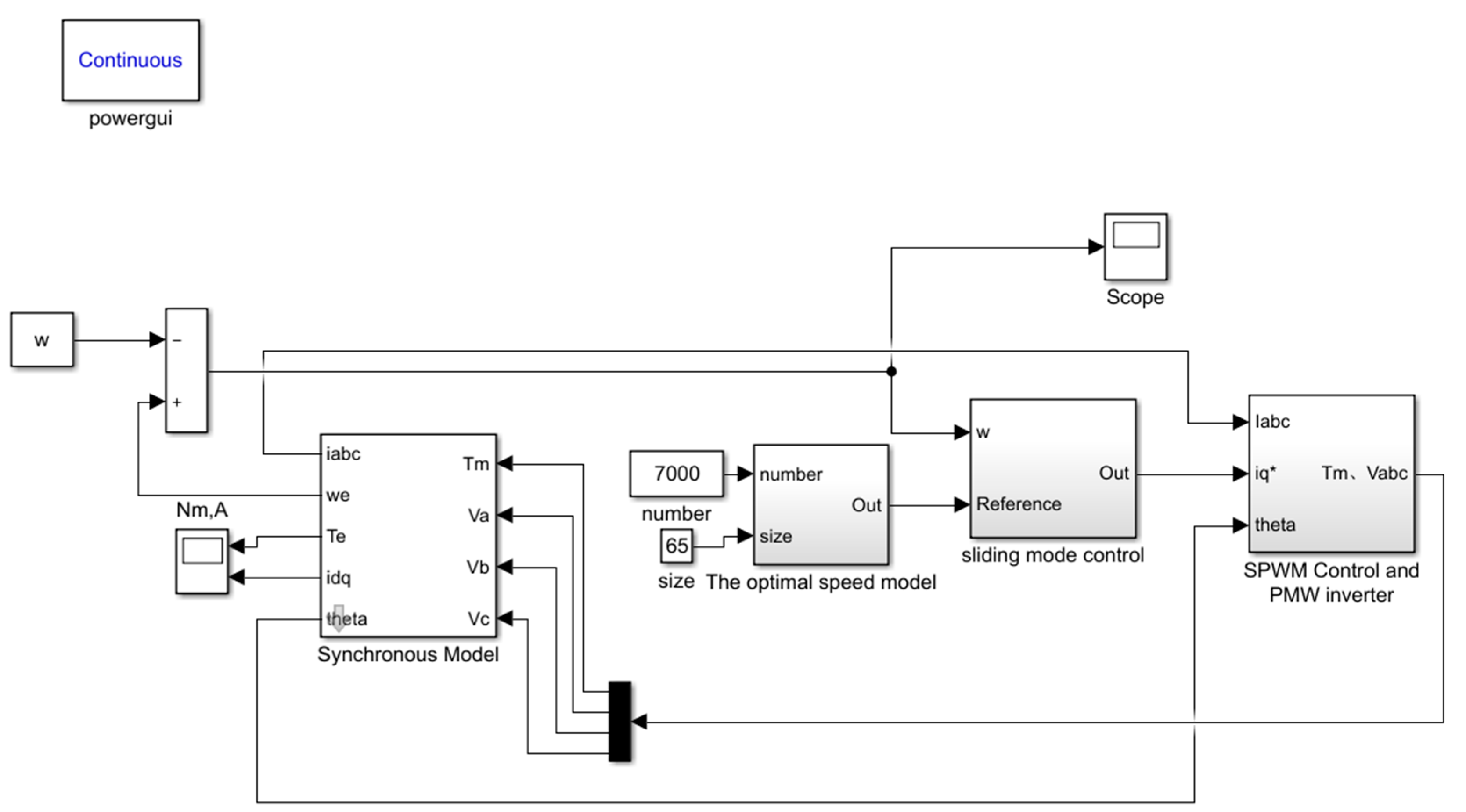
The model of the SAG mill motor and sliding mode control was built in the MATLAB Simulink platform as shown in Figure 10.
The left side of the model is the power system graphical user interface module. In this model, for the convenience of calculation, the motor model is the international system unit, and the input of the motor is rotor speed. The right side of the model is the sliding mode control module.
In this study, k = 5 and ε = 0.1 were used for simulation experiments under different working conditions. In the simulation experiment, it was assumed that the gear ratio of the large and small gears is 30. Meanwhile, it was assumed that
Simulation under different conditions was carried out. The results are as follows:
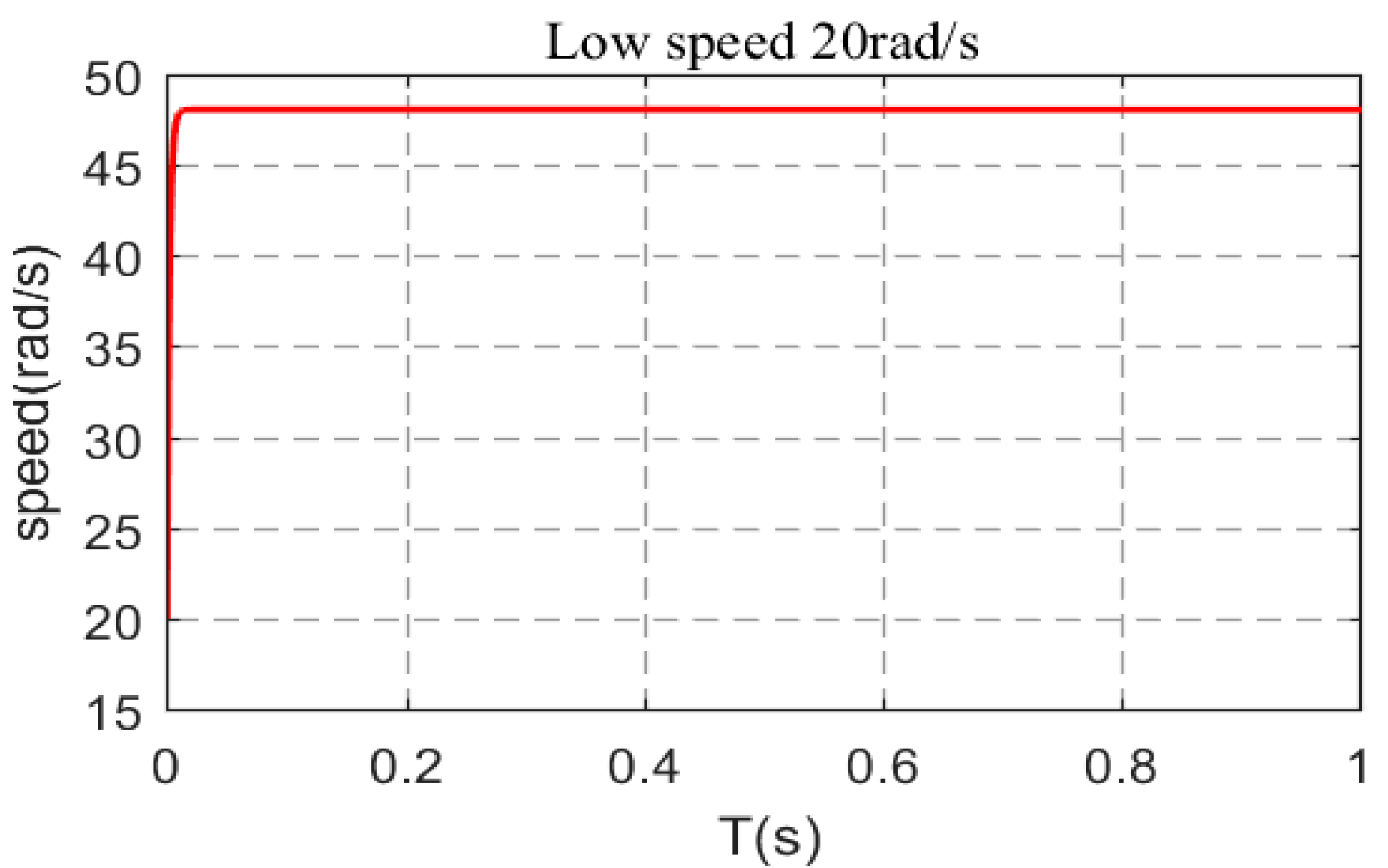
1. Under low speed condition,
The initial rotor speed was set at 20 rad/s, number of particles was 7000, and particle size was 65 mm. At this time, the optimal rotational speed calculated by Equation (13) is 1.582 rad/s. The gear ratio is 30, and the expected speed of the motor is 47.46 rad/s. The simulation result is shown in Figure 11. It shows that when time is zero and the motor speed is 20 rad/s, it reaches the target speed in a short period of time and tends to be stable.
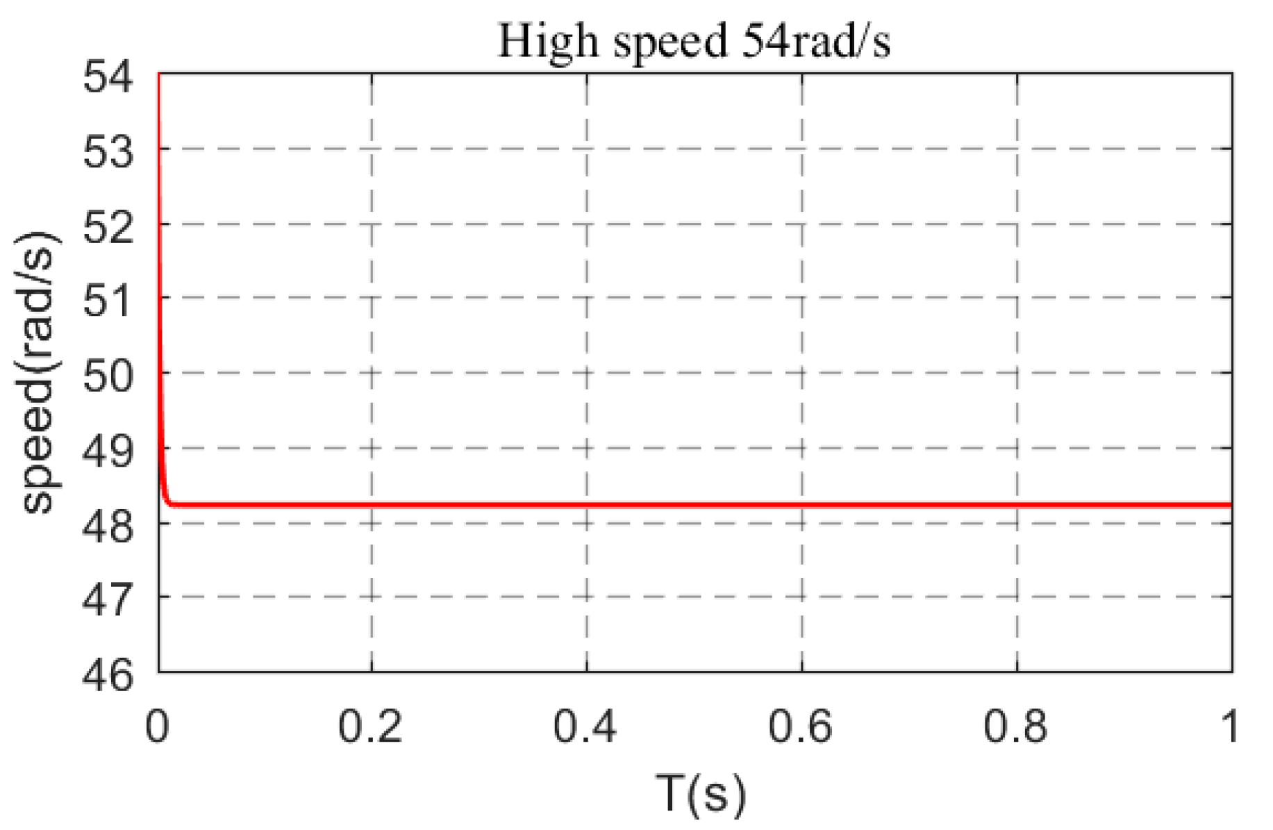
2. Under high speed condition
The initial speed of the rotor was 54 rad/s, number of particles was 9000, and particle size was 60 mm. The optimal rotational speed result calculated by Equation (13) is 1.607 rad/s. The expected speed of the motor is 48.22 rad/s. The simulation result is shown in Figure 12. It shows that the speed reaches the target speed in a short period of time and tends to be stable.
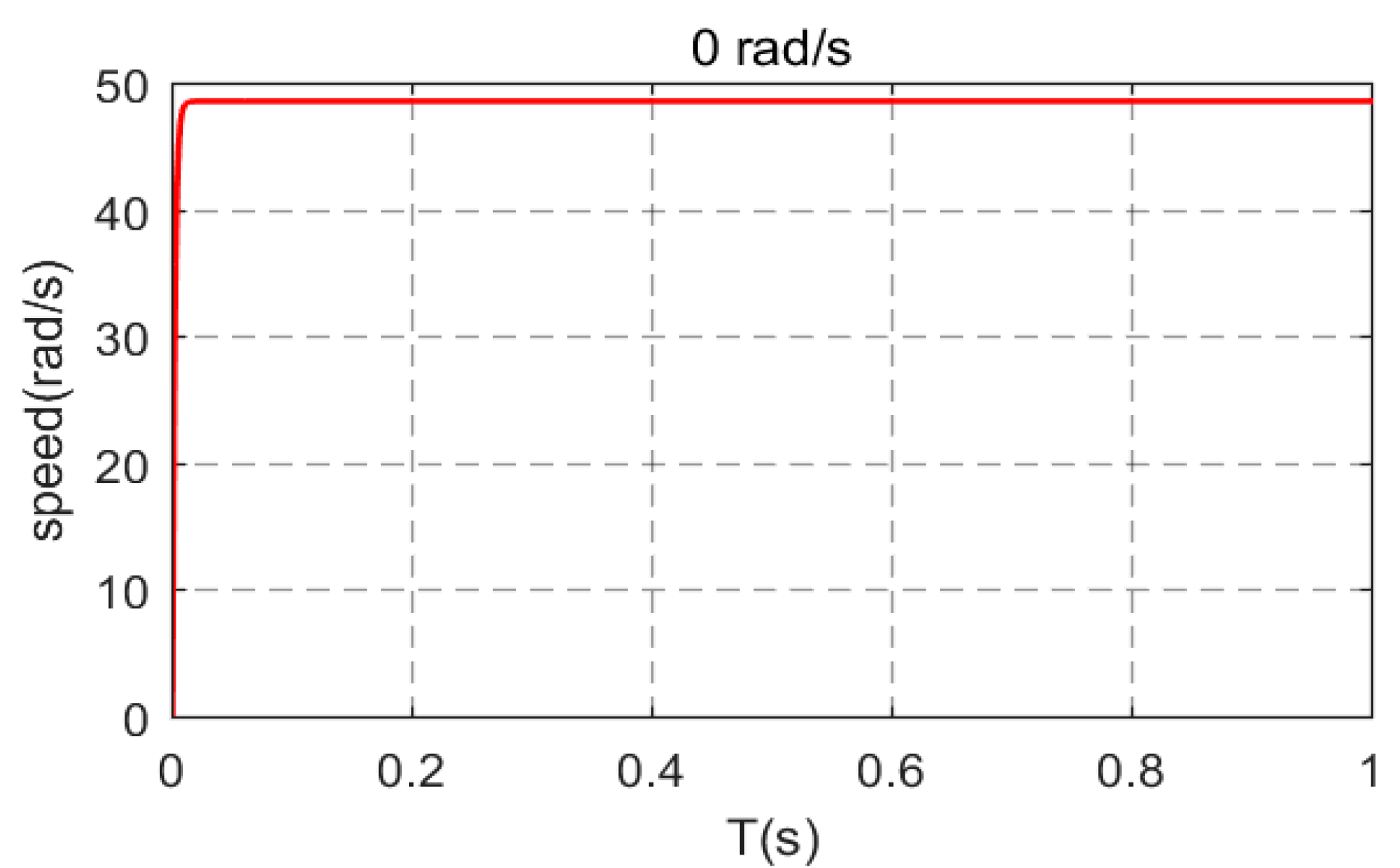
3. The motor starting process
The number of particles was set as 7500, and particle size was 90mm. The optimal speed from Equation (13) is 1.637 rad/s, and the expected speed of the motor is 49.1 rad/s. The simulation results are shown in Figure 13. It shows that when time is zero, the motor speed is zero, then the speed reaches the target speed in a short period of time and tends to be stable.
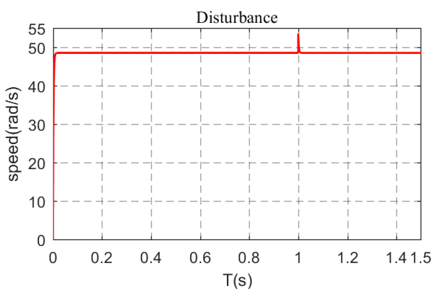
4. Disturbance of motor under stable operation condition
As we know from Figure 11, Figure 12 and Figure 13, the designed sliding mode control begins to converge to the desired speed and tends to be stable in approximately 0.1 s. When the time is 1 s, it gives the motor a step disturbance. The results are shown in Figure 14. They show that under the effect of sliding mode control, the motor speed can still return to the desired speed for movement in a short period of time.
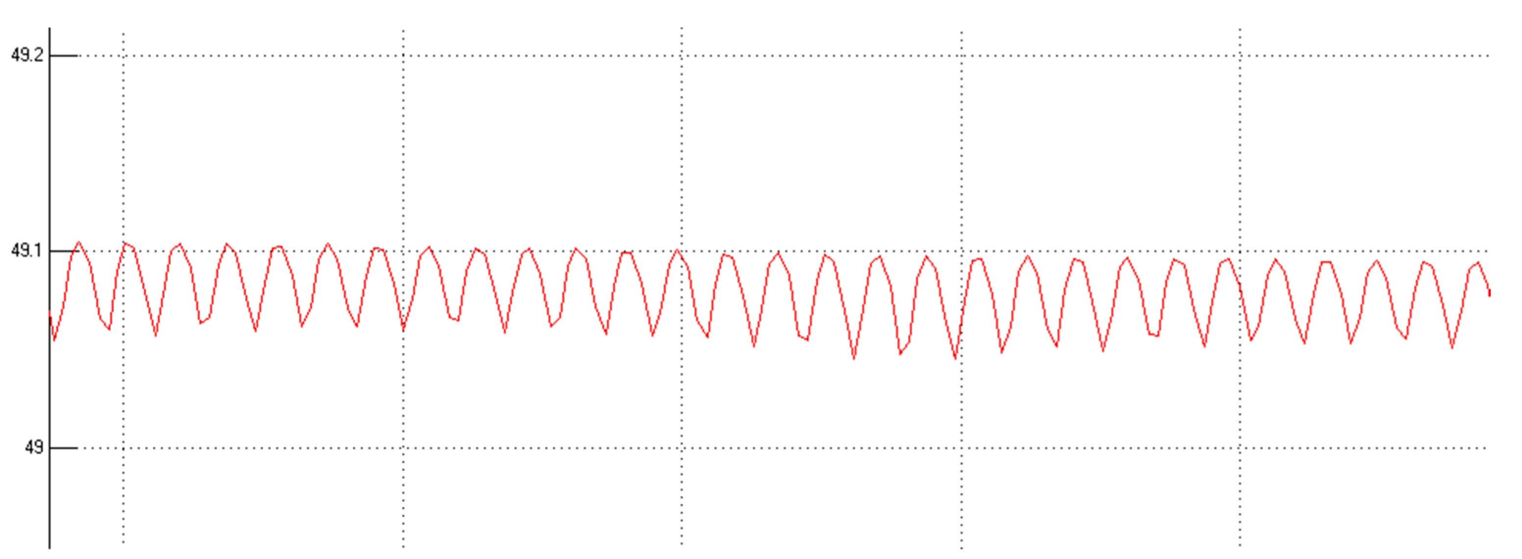
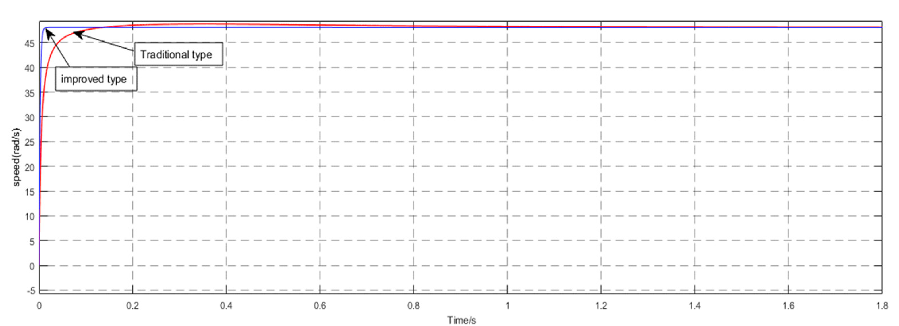
Regardless of whether the initial speed is too high or too low, the target speed can be reached in approximately 0.1 s under the designed sliding mode control as shown in Figure 11, Figure 12, Figure 13 and Figure 14, which show that the sliding mode control designed in this experiment is feasible for the speed control of the SAG mill motor, and the motor can quickly become stable. When the motor runs stably, the chattering is less than 0.1 rad/s as shown in Figure 15, which shows that there is less chattering, and the operation is stable. Finally, the simulation results of the improved exponential approaching law were compared with the traditional exponential approaching law as shown in Figure 16. The comparison shows that the improved exponential approaching law has faster approach speed and less chattering compared with the traditional exponential approaching law.
5. Conclusions
The model of the SAG mill was established by using the discrete element simulation software EDEM. Simulation of internal medium motion at different speeds under different particle numbers and particle sizes was carried out. The following conclusions can be drawn:
- In the case of constant particle size, as the number of particles increases, the optimal speed generally increases slowly.
- In the case of the same number of particles, the optimal rotation speed generally increases slowly with the increase of the particle size but decreases slightly after a certain value, which indicates that when the particle size is too large, increasing the mill speed does not necessarily improve the grinding effect.
- By analyzing the response surface, the effect of the number of particles on the optimal rotation speed is greater than the effect of the particle size.
- The designed, improved sliding mode control enables the motor to run at the target speed quickly with less chattering and stable operation.
In this study, the influence of the number of particles and particle size on the optimal speed in the designed experiment was analyzed. However, there are still some factors that need additional consideration. First of all, in the actual production process, the ore fed into the mill is inconsistent in hardness, shape size, metal content, and water content, which is related to the composition and structure of the ore and is difficult to change by artificial means. These factors are not reflected in the experiment. Secondly, the height and shape of the liner in the mill, as well as the wear that exists during the grinding process, also have an effect on the grinding. However, these factors were not taken into consideration.
Author Contributions
Formal analysis, J.Y.; investigation, X.W., Z.Z.; methodology, Z.Z., X.W. and C.Y.; resources, X.W., C.Y. and Z.Z.; supervision, X.W.; Writing—Original draft, J.Y.; Writing—Review and editing, J.Y, X.W. All authors read and approved the final version of the manuscript.
Funding
This research was supported by the National Natural Science Foundation of China (No. 61673401) and the 111 projects (No. B17048).
Conflicts of Interest
The authors declare no conflict of interest.
References
- Salazar, J.; Valdés-González, H.; Vyhmesiter, E.; Cubillos, F. Model predictive controlof semi-autogenous mills(sag). Miner. Eng. 2014, 64, 92–96. [Google Scholar] [CrossRef]
- Hasankhoeia, A.R.; Maleki-Moghaddamb, M.; Haji-Zadehc, A.; Barzgard, M.E.; Banisi, S. On dry SAG mills end liners: Physical modeling, DEM-based characterization and industrial outcomes of a new design. Miner. Eng. 2019, 141, 1–17. [Google Scholar] [CrossRef]
- Gaipin, C.; Buchun, Q.; Xianhuang, X. Numerical Simulation and Experimental Study on Grinding Effect of SAG. Master’s Thesis, Henan Polytechnic University, Henan, China, 2017. [Google Scholar]
- Joachim, H. Control of Large Salient-Pole Synchronous Machines Using Synchronous Optimal Pulse width Modulation. IEEE Trans. Ind. Appl. 2015, 62, 3372–3379. [Google Scholar]
- Cleary, P.; Owen, P. Effect of operating condition changes on the collisional environment in a SAG mill. Miner. Eng. 2019, 132, 297–315. [Google Scholar] [CrossRef]
- Rodríguez, J.R.; Pontt, J. Technical Evaluation and Practical Experience of High-Power Grinding Mill Drives in Mining Applications. IEEE Trans. Ind. Appl. 2005, 41, 866–874. [Google Scholar] [CrossRef]
- Hadizadeh, M.; Farzanegan, A.; Noaparast, M. A plant-scale validated MATLAB-based fuzzy expert system to control SAG mill circuits. J. Process Control 2018, 70, 1–11. [Google Scholar] [CrossRef]
- Palavicino, P.C.; Valenzuela, M.A. Modeling and Evaluation of Cycloconverter-Fed, Two-Stator Windings SAG Mill Drive. Part II: Starting Evaluation. IEEE Trans. Ind. Appl. 2014, 51, 2582–2589. [Google Scholar] [CrossRef]
- Castro, P.P.; Valenzuela, M.A. Space Vector Modeling of a SAG Mill Drive and Evaluation during Mill Shutdowns. In Proceedings of the IEEE Industry Application Society Annual Meeting, Addison, TX, USA, 18–22 October 2015. [Google Scholar]
- José, G.H.; Benjamin, R.; Villalobos, E.; JoséOlivares, F. Robust Multivariable Predictive Control Strategy on SAG Mills; Codelco Chile—Division El Teniente. IFAC 2009, 42, 49–54. [Google Scholar]
- Fayez, F.M. Adaptive dynamic sliding-mode control system using recurrent RBFN for high-performance induction motor servo drive. IEEE Trans. Ind. Inform. 2013, 9, 1922–1936. [Google Scholar]
- Steyn, C.W.; Sandrock, C. Benefits of optimisation and model predictive control on a fully autogenous mill with variable speed. Miner. Eng. 2013, 53, 113–123. [Google Scholar] [CrossRef] [Green Version]
- Lai, C.K.; Shyu, K.K. A novel motor drive design for incremental motion system via sliding-mode control method. IEEE Trans. Ind. Electron. 2005, 52, 499–507. [Google Scholar] [CrossRef]
- Boiko, L.M. Chattering in sliding mode control systems with boundary layer approximation of discontinuous control. Int. J. Syst. Sci. 2013, 44, 1–8. [Google Scholar] [CrossRef]
- Wu, C.Y. Discrete Element Modelling of Particulate Media; Royal Society of Chemistry: Cambridge, UK, 2012. [Google Scholar]
- Cleary, P.W.; Cohen, R.C.Z.; Harrison, S.M.; Sinnott, M.D.; Prakash, M.; Mead, S. Prediction of industrial, biophysical and extreme geophysical flows using particle methods. Eng. Comput. 2013, 30, 157–196. [Google Scholar]
- Zhu, H.P.; Zhou, R.Y.; Yang, Z.Y.; Yu, A.B. Discrete particle simulation of particulate systems: A review of major applications and findings. Chem. Eng. Sci 2008, 63, 5728–5770. [Google Scholar] [CrossRef]
- Mishra, B.K.; Rajamani, R.K. The discrete element method for the simulation of ball mills. Appl. Math. Model 1992, 16, 598–604. [Google Scholar] [CrossRef]
- Cleary, P.W.; Sawley, M.L. DEM modelling of industrial granular flows: 3D case studies and the effect of particle shape on hopper discharge. Appl. Math. Model 2002, 26, 89–111. [Google Scholar] [CrossRef]
- Cleary, P.W. Modelling comminution devices using DEM. Int. J. Numer. Anal. Methods Geomech. 2001, 25, 83–105. [Google Scholar] [CrossRef]
- Cleary, P.W. Recent advances in DEM modelling of tumbling mills. Miner. Eng. 2001, 14, 1295–1319. [Google Scholar] [CrossRef]
- Weerasekara, N.S.; Liu, L.X.; Powell, M.S. Estimating energy in grinding using DEM modelling. Miner. Eng. 2016, 85, 23–33. [Google Scholar] [CrossRef] [Green Version]
- Weerasekara, N.S.; Powell, M.S.; Cleary, P.W. The contribution of DEM to the science of comminution. Powder Technol. 2013, 248, 3–24. [Google Scholar] [CrossRef]
- Savkoor, A.R.; Briggs, G. The effect of tangential force on contact of elastic solids in adhesion. Proc. R. Soc. Lond. A 1971, 365, 103–114. [Google Scholar]
- Zhang, X.G.; Sun, L.; Zhao, K. Sliding mode control of PMSM based on a novel load torque sliding mode observer. Proc. CSEE 2012, 32, 111–116. [Google Scholar]
- Dong, G.; Venkata, D. Sliding Mode High Speed Control of PMSM for Electric Vehicle Based on Flux-weakening Control Strategy. In Proceedings of the 36th Chinese Control Conference, Dalian, China, 26–28 July 2017. [Google Scholar]
Figure 1.
The schematic diagram of the working principle of a semi-autogenous (SAG) mill.

Figure 2.
Three types of grinding balls: (a) cascading type; (b) throwing type; (c) centrifugal type.
Figure 2.
Three types of grinding balls: (a) cascading type; (b) throwing type; (c) centrifugal type.

Figure 3.
Force equilibrium of the grinding medium.

Figure 4.
Trajectory of the grinding medium.

Figure 5.
Model of the roller.

Figure 6.
NZ value recorded: (a) number of particles in each small area of the dropping area; (b) the number of particles dropped in the whole dropping area.
Figure 6.
NZ value recorded: (a) number of particles in each small area of the dropping area; (b) the number of particles dropped in the whole dropping area.

Figure 7.
Relationship between the optimal speed and different parameters: (a) the optimal speed and the number of particles; (b) the optimal speed and particle size.
Figure 7.
Relationship between the optimal speed and different parameters: (a) the optimal speed and the number of particles; (b) the optimal speed and particle size.

Figure 8.
Three-dimensional surface diagram of the response surface.

Figure 9.
The contour map of the response surface.

Figure 10.
Motor model of the SAG mill and sliding mode control.

Figure 11.
Results of sliding mode control under low speed.

Figure 12.
Results of sliding mode control under high speed.

Figure 13.
Results of sliding mode control under starting process.

Figure 14.
Results of speed response in the case of sudden disturbance.

Figure 15.
Stability of motor speed under sliding mode control.

Figure 16.
Comparison of the response of improved and traditional exponential approaching law.


Table 1.
Simulation conditions of discrete element method (DEM).
| Simulation Parameters | Particle Materials | Steel Balls |
|---|---|---|
| Poisson’s ratio | 0.3 | 0.3 |
| Shear Modulus | 2.3 × 10⁷ Pa | 1 × 10¹⁰ Pa |
| Density | 2678 kg/m3 | 7850 kg/m3 |
Table 2.
Values of parameters for cross-over test.
| Size(mm) | Number | Speed (rad/s) |
|---|---|---|
| 50 | 5000 | 1.28 (50%nc) |
| 55 | 5500 | 1.285 |
| 60 | 6000 | 1.29 |
| … | … | … |
| 90 | 9500 | 1.64 (90%nc) |
| 95 | 10,000 | none |
| 100 | 12,500 | none |
| none | 15,000 | none |
Table 3.
Variance analysis.
| Cause of Variance | Sum of Squares | Degrees of Freedom | Standard Deviation | Value of F | p > F |
|---|---|---|---|---|---|
| Model | 1.449 × 10⁻³ | 5 | 2.897 × 10⁻⁴ | 3.40 | 0.0470 |
| A | 8.091 × 10⁻⁴ | 1 | 8.091 × 10⁻⁴ | 9.50 | 0.0116 |
| B | 4.005 × 10⁻⁴ | 1 | 4.005 × 10⁻⁴ | 4.70 | 0.0453 |
| AB | 1.622 × 10⁻⁴ | 1 | 1.622 × 10⁻⁴ | 1.91 | 0.0475 |
| A2 | 8.377 × 10⁻⁷ | 1 | 8.377 × 10⁻⁷ | 9.838 × 10⁻³ | 0.0922 |
| B2 | 1.092 × 10⁻⁵ | 1 | 1.092 × 10⁻⁵ | 0.13 | 0.0277 |
| Residual | 8.514 × 10⁻³ | 1 | 8.514 × 10⁻³ | none | none |
| Lack of fit | 2.300 × 10⁻³ | 1 | none | none | none |
© 2020 by the authors. Licensee MDPI, Basel, Switzerland. This article is an open access article distributed under the terms and conditions of the Creative Commons Attribution (CC BY) license (http://creativecommons.org/licenses/by/4.0/).
Share and Cite
MDPI and ACS Style
Wang, X.; Yi, J.; Zhou, Z.; Yang, C. Optimal Speed Control for a Semi-Autogenous Mill Based on Discrete Element Method. Processes 2020, 8, 233. https://0-doi-org.brum.beds.ac.uk/10.3390/pr8020233
AMA Style
Wang X, Yi J, Zhou Z, Yang C. Optimal Speed Control for a Semi-Autogenous Mill Based on Discrete Element Method. Processes. 2020; 8(2):233. https://0-doi-org.brum.beds.ac.uk/10.3390/pr8020233
Chicago/Turabian StyleWang, Xiaoli, Jie Yi, Ziyu Zhou, and Chunhua Yang. 2020. "Optimal Speed Control for a Semi-Autogenous Mill Based on Discrete Element Method" Processes 8, no. 2: 233. https://0-doi-org.brum.beds.ac.uk/10.3390/pr8020233
Note that from the first issue of 2016, this journal uses article numbers instead of page numbers. See further details here.