Considering the Diffusive Effects of Cavitation in a Homogeneous Mixture Model

Abstract

Homogeneous mixture models are widely used to predict the hydrodynamic cavitation. In this study, the constant-transfer coefficient model is implemented into a homogeneous cavitation model to predict the heat and mass diffusion. Modifications are made to the average bubble temperature and the Peclet number for thermal diffusivity in the constant-transfer coefficient model. The evolutions of a spherical bubble triggered by negative pressure pulse are simulated to evaluate the prediction of heat and mass diffusion by the homogeneous model. The evolutions of three bubbles inside a rectangular tube are simulated, which show good accuracy of the homogeneous model for multibubbles in stationary liquid.

1. Introduction

Cavitation is usually caused by pressure decrease, leading to the growth of bubbles and followed by their rapid collapse. During the bubble growth, the temperature inside the bubble decreases and heat transfer occurs. Meanwhile, evaporation occurs at the bubble wall and vapor diffuses into the bubble. The heat and mass transfer make it complex to accurately predict the bubble dynamics [1,2,3]. Interface capturing methods, such as VOF and level set, can accurately predict the dynamics of pure gas bubbles [4]. However, they are inapplicable when there are huge number of bubbles. Instead, homogeneous models are widely used to simulate the hydrodynamic cavitation.

Homogeneous models usually use the Rayleigh–Plesset-type equations to predict the bubble dynamics [5,6,7,8,9,10,11,12,13]. Usually, only the local pressure but not the far-field pressure is known for numerical simulations. Ye et al. [14] proposed a homogeneous mixture model based on the bounded Rayleigh–Plesset equation [15]. This model solves the bubble dynamics using the local pressure, and can accurately predict the bubble dynamics of an isothermal gas bubble before bubble rebound. As some other homogeneous models [16,17,18], the heat transfer is simply treated by setting the polytropic index to be a constant and the mass transfer is simply treated by assuming the vapor pressure to be constant. Different working conditions need different constants. It is almost impossible to accurately predict the heat and mass transfer by estimating proper constants. These treatments of heat and mass transfer need to be improved.

Preston et al. [19] proposed a theoretical model named constant-transfer coefficient model, which can capture the effect of heat and mass transfer efficiently for a spherical bubble. In this model, two transport equations are used to, respectively, record the pressure (p_GV) and the mass of vapor (m_V) inside the bubble, and two constant-transfer coefficients are used to estimate the heat and mass flux at the bubble wall. In this study, this model is implemented into the homogeneous mixture model proposed by Ye et al. [14], and the calculations of the average bubble temperature and the Peclet number for thermal diffusivity in the constant-transfer model are modified. In the validation part, the evolutions of a spherical bubble triggered by pressure pulse are simulated and the evolutions of three bubbles in a regular arrangement are simulated to evaluate the accuracy for multibubbles. Comparisons with the predictions by the VOF method and the full computation (uses six equations to predict the heat and mass transfer) are made.

2. Mathematical Model

2.1. Homogeneous Mixture Cavitation Model

The homogeneous mixture model proposed by Ye et al. [14] is based on the bounded Rayleigh–Plesset equation [15] as follows:

$$R\left(1-\frac{R}{R_e}\right)\ddot{R}+\left(1.5-\frac{2R}{R_e}+\frac{R^4}{2R_e^4}\right)\dot{R^2}=\frac{p_b-p_e}{{\rho }_{\mathrm{L}}}$$

(1)

where R is the bubble radius, the over dot denotes the derivative in time, p_b is the liquid pressure at the bubble surface, p_e is the pressure at r = R_e, and ρ_L is the liquid density. $\ddot{R}$ of a 3D spherical bubble is predicted by [14]:

$$\ddot{R}=\frac{\raisebox{1ex}{$p_b-p$}\!\left/ \!\raisebox{-1ex}{${\rho }_{\mathrm{L}}$}\right.+\left(0.4{\alpha }^{7/3}-1.3{\alpha }^{4/3}+2.4{\alpha }^{1/3}-1.5\right){\dot{R}}^2}{\left(1+0.2{\alpha }^{4/3}-1.2{\alpha }^{1/3}\right)R}$$

(2)

where p is the local pressure and α is the volume fraction of gas–vapor mixture. In order to improve the numerical stability, a minimum collapse rate ${\dot{R}}_{\min }$= −30 m/s is given, below which the collapse rate will not decrease any more, by the modification of $\ddot{R}$ as:

$${\ddot{R}}_{\mathrm{m}}=\{\begin{array}{c}\ddot{R} \mathrm{when} \dot{R}\ge {\dot{R}}_{\min }\\ \max \left(\ddot{R},0\right) \mathrm{when} \dot{R}<{\dot{R}}_{\min }\end{array}$$

(3)

p_b can be determined by:

$$p_b=p_{\mathrm{V}}+\left(p_0+\frac{2S}{R_0}-p_{s0}\right){\left(\frac{R_0}{R}\right)}^{3\gamma }-\frac{2S}{R}-\frac{4{\mu }_{\mathrm{L}}\dot{R}}{R}$$

(4)

where the subscripts V and 0, respectively, denote the vapor and the initial value, p₀ is the initial pressure outside the bubble, p_s0 is the initial vapor saturation pressure, R₀ is the initial bubble radius, γ is the polytropic index, S denotes the surface tension coefficient, and μ_L is the dynamic viscosity of liquid. γ = 1 for an isothermal process while γ =$\kappa$ (adiabatic exponent) for an adiabatic process. Usually, p_V is simply supposed to be equal to p_s0, and γ is set to be a constant between 1 and $\kappa$. In this study, the pressure inside the bubble p_GV (the subscript G denotes the noncondensable gas) will be predicted by the constant-transfer coefficient model [19].

2.2. Constant-Transfer Coefficient Model

The constant-transfer coefficient model [19] is a theoretical model for spherical bubble dynamics that considers the effects of heat and mass transfer. Several assumptions were made: (1) the gas–vapor mixture was a perfect gas, (2) constant transport properties and surface tension coefficient, (3) thermal equilibrium and vapor-pressure equilibrium at the gas–liquid interface, (4) p_GV was spatially uniform, (5) the liquid temperature was uniform, (6) no diffusion of noncondensable gas in the liquid, and (7) the liquid was “cold.”

Two transport equations are used to, respectively, predict p_GV and m_V. All variables were non-dimensionalized in Ref. [19], which are converted into dimensional form in this study. The initial p_GV is determined as:

$$p_{\mathrm{GV}0}=p_0+\frac{2S}{R_0}$$

(5)

The source term of the transport equation of p_GV is determined by:

$$\frac{d{p}_{\mathrm{GV}}}{dt}=-\frac{3{\kappa }_{\mathrm{w}}}{R}(p_{\mathrm{GV}}\dot{R}-\frac{{ℛ}_0{k}_{\mathrm{w}}}{c_{p0}R}{\frac{\partial T}{\partial y}|}_{y=1}-\frac{{ℛ}_{\mathrm{V}}{D}_0{p}_{\mathrm{GV}}}{ℛ\left(1-C_{\mathrm{w}}\right)R}{\frac{\partial C}{\partial y}|}_{y=1})$$

(6)

where T is the temperature, C is the mass fraction of vapor, the subscript w denotes the value at the bubble wall, ${\kappa }_{\mathrm{w}}=C_{\mathrm{w}}{\kappa }_{\mathrm{V}}+\left(1-C_{\mathrm{w}}\right){\kappa }_{\mathrm{G}}$ $\left({\kappa }_{\mathrm{V}}=4/3,{\kappa }_{\mathrm{G}}=1.4\right)$, k_w = $C_{\mathrm{w}}{k}_{\mathrm{V}}$ + $\left(1-C_{\mathrm{w}}\right)k_{\mathrm{G}}$, and $ℛ$ = $C_{\mathrm{w}}{ℛ}_{\mathrm{V}}$ + $\left(1-C_{\mathrm{w}}\right){ℛ}_{\mathrm{G}}$ are, respectively, the adiabatic exponent, thermal conductivity, and perfect gas constant of the gas–vapor mixture at the bubble wall, and c_p0 and D₀ are, respectively, the specific heat and the diffusivity of initial gas–vapor mixture. Since the vapor pressure at the bubble wall is assumed to be in equilibrium, C_w can be obtained by:

$$C_{\mathrm{w}}=\frac{p_{s0}{M}_{\mathrm{V}}}{p_{s0}{M}_{\mathrm{V}}+\left(p_{\mathrm{GV}}-p_{s0}\right)M_{\mathrm{G}}}$$

(7)

where M is the molecular weight. The gradients of C and T at the bubble wall are modeled using constant-transfer coefficients β_C and β_T as [19]:

$${\frac{\partial C}{\partial y}|}_{y=1}\approx {\beta }_C\left(C_{\mathrm{w}}-\overline{C}\right)$$

(8)

$${\frac{\partial T}{\partial y}|}_{y=1}\approx {\beta }_T\left(T_0-\overline{T}\right)$$

(9)

where $\overline{C}\approx m_{\mathrm{V}}/\left(m_{\mathrm{G}0}+m_{\mathrm{V}}\right)$ is the average vapor mass fraction, T₀ is the initial temperature, and $\overline{T}$ is the average bubble temperature estimated by Preston et al. [19] as:

$$\overline{T}\approx \frac{p_{\mathrm{GV}}{R}^3{T}_0}{p_{\mathrm{GV}0}{R}_0^3}\frac{m_{\mathrm{G}0}+m_{\mathrm{V}0}}{m_{\mathrm{G}0}+m_{\mathrm{V}}}$$

(10)

According to the perfect gas law, it is modified to:

$$\overline{T}\approx \frac{p_{\mathrm{GV}}{R}^3{T}_0}{p_{\mathrm{GV}0}{R}_0^3}\frac{m_{\mathrm{G}0}{ℛ}_{\mathrm{G}}+m_{\mathrm{V}0}{ℛ}_{\mathrm{V}}}{m_{\mathrm{G}0}{ℛ}_{\mathrm{G}}+m_{\mathrm{V}}{ℛ}_{\mathrm{V}}}$$

(11)

β_C and β_T are obtained by linear analysis as [19]:

$${\beta }_C=\mathsf{ℛ}\left\{\mathsf{\Psi }\left(P{e}_G\right)\right\}$$

(12)

$$P{e}_G=R_0^2{\mathsf{\Omega }}_0/D_0$$

(13)

$${\beta }_T=\mathsf{ℛ}\left\{\mathsf{\Psi }\left(P{e}_T\right)\right\}$$

(14)

$$P{e}_T={\rho }_{\mathrm{GV}0}{c}_{p0}{R}_0^2{\mathsf{\Omega }}_0/k_{\mathrm{GV}0}$$

(15)

$$\mathsf{\Psi }\left(Pe\right)={\left(\frac{1}{\sqrt{Pe·i}\coth \sqrt{Pe·i}-1}-\frac{3}{Pe·i}\right)}^{-1}$$

(16)

where Pe_G and Pe_T are, respectively, the Peclet numbers for mass and thermal diffusivity, ρ_GV0 is the initial density of gas–vapor mixture, and Ω₀ is the bubble natural frequency determined by:

$${\mathsf{\Omega }}_0=\sqrt{\frac{3\left(p_0-p_{s0}\right)+4S/R_0}{{\rho }_{\mathrm{L}}{R}_0^2}}$$

(17)

m_V is predicted by another transport equation, whose source term is as follows:

$$\frac{{dm}_{\mathrm{V}}}{dt}=4\pi R\frac{D_0{p}_{\mathrm{GV}}}{ℛ\left({1-C}_{\mathrm{w}}\right)T_0}{\frac{\partial C}{\partial y}|}_{y=1}$$

(18)

The initial m_V and m_G are determined as:

$$m_{\mathrm{V}0}=\frac{4}{3}\pi R_0^3{\rho }_{\mathrm{V}0}$$

(19)

$$m_{\mathrm{G}0}=\frac{4}{3}\pi R_0^3{\rho }_{\mathrm{G}0}$$

(20)

When p_GV is obtained, p_b is determined as follows instead of Equation (4):

$$p_{\mathrm{b}}=p_{\mathrm{GV}}-\frac{2S}{R}-\frac{4{\mu }_{\mathrm{L}}\dot{R}}{R}$$

(21)

3. Validation

The validation cases are similar to those in [19]. A spherical bubble is triggered by a negative pressure pulse. The gravity is neglected and the flows are assumed to be laminar. T₀ is 298 K and the negative pressure pulse takes the following form:

$$p=p_0\left(1-{\mathrm{A}}_p·e^{-{\left(t/t_{\mathrm{w}}-3\right)}^2}\right)$$

(22)

Table 1. Parameters for the validation cases of the spherical bubble triggered by the negative pressure pulse in Equation (22) at the distance of R_e.

Case	R0 (μm)	Re (mm)	p0 (kPa)	ps0 (Pa)	S (N/m)	Ω0 (kHz)	βT	βC	Ap	tw (s)
A	10	5	101.325	0	0	1746	5.15	-	1	10−4
B	40	5	20	0	0	193.9	5.02	-	1	10−4
C	40	5	50	0	0	306.6	5.28	-	1	10−4
D	40	5	101.325	0	0	436.5	6.46	-	1	10−4
E	40	5	200	0	0	613.3	9.03	-	1	10−4
F	40	5	500	0	0	969.7	15.7	-	1	10−4
G	40	5	800	0	0	1227	21.4	-	1	10−4
H	100	5	101.325	0	0	174.6	8.69	-	1	10−4
I	40	1000	101.325	3142	0.072	434.9	6.56	6.21	0.985	10−4
J	40	1000	101.325	3142	0.072	434.9	6.56	6.21	0.97	10−3

shows the parameters of these validation cases. Cases A to H simulate the evolutions of a pure gas bubble to evaluate the prediction of heat transfer. The negative pressure pulse is employed at the distance of R_e = 5 mm away from the bubble (Figure 1). Comparisons are made with the predictions by the VOF method since it can accurately predict the heat transfer. For better comparison, the surface tension is neglected. Before the comparison, all these cases are simulated under the isothermal assumption to validate the accuracy of the VOF method and homogeneous model without heat transfer, by comparing with the theoretical results predicted by Equation (1). Results show that the relative differences between the predicted maximum bubble radius by the VOF method and Equation (1) are less than 0.1%, and those between the homogeneous model and Equation (1) are less than 0.22%. After the comparisons of one bubble, the validation case of three bubbles [14] is simulated to evaluate the homogeneous model for multibubbles.

Cases I and J simulate the evolution of a gas–vapor bubble to include the mass transfer. Since it is complex to consider the phase change for the VOF method, comparisons are made with the theoretical results by the full computation [19] and constant-transfer coefficient model. It should be clarified that R_e = ∞ in the prediction by the full computation, while R_e = 1 m in the prediction by the constant-transfer coefficient model and homogeneous model. In order to prove the independency of R_e, the dynamics of a pure gas bubble with R_e = 1 m and ∞ are simulated by Equation (1) under the isothermal assumption; the relative difference of R_max between them is only 0.001%.

3.1. Gas Bubbles

Figure 1 shows the 2D computational grid for the homogeneous mixture model, which contains 1718 quadrilateral meshes. R_max decreases by 0.11% for case D when the grid number is increased to 5087. The bubble is located at the lower-left corner of the computational domain. Since there is only one bubble, a virtual initial bubble number density (n₀) of 10⁹ m⁻³ is given inside the region with the radius of ${\left(4\pi n_0/3\right)}^{-1/3}$ (marked in red in Figure 1). Additionally, the initial gas volume fraction inside this region is $4\pi n_0{R}_0^3/3$, which makes the total gas volume equal to $4\pi R_0^3/3$. When using the VOF method, special contractions of the mesh are applied around the bubble, and the grid number is about eight times larger. R_max only increases by 0.019% for case D when the grid size around the bubble is further decreased by 33%.

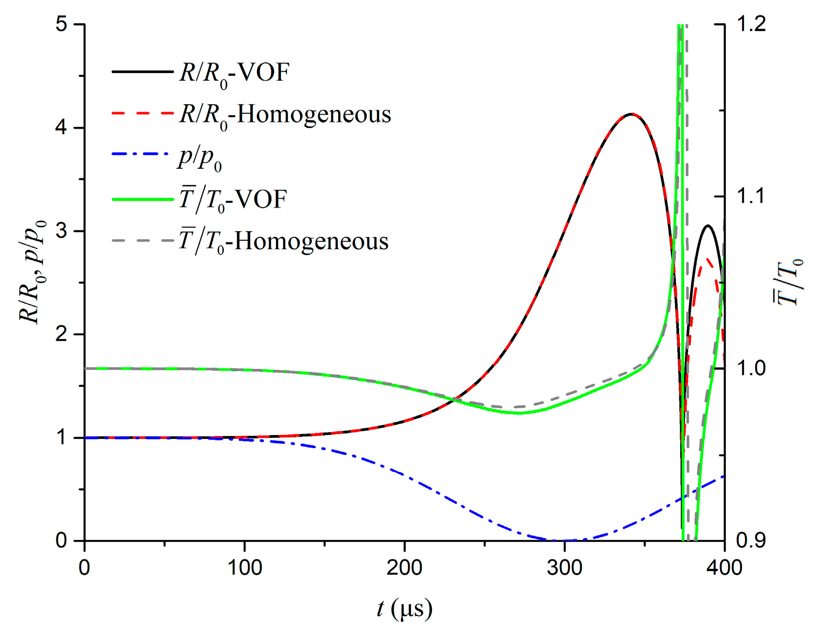
Figure 2 compares R and $\overline{T}$ of case D predicted by the VOF method and homogeneous model. Both R and $\overline{T}$ are a little overpredicted by the homogeneous model before bubble rebound, and ${\delta }_{R\max }$ (the relative difference of R_max predicted by the homogeneous model and VOF method) is only 0.18%. The dependences of ${\delta }_{R\max }$ on R₀, t_w, and p₀ are analyzed based on case D, which are shown in Figure 3. Cases A, D, and H are used to analyze the influence of R₀, while cases B to G are used to analyze the influence of p₀. It can be seen from Figure 3a that ${\delta }_{R\max }$ increases with R₀, and ${\delta }_{R\max }$ < 1% when R₀ ≤ 100 μm (the nucleus radius is usually smaller than 100 μm). It can be seen from Figure 3b that ${\delta }_{R\max }$ also increases with p₀, and it reaches 4.1% at 800 kPa, which means the heat transfer is obviously overpredicted. In order to reduce the heat transfer at large p₀, the calculation of Pe_T (Equation (15)) is modified by fixing p₀ to the atmospheric pressure. After this modification, ${\delta }_{R\max }$ at 800 kPa decreases to 1.1%, much smaller than the original value. It can be seen from Figure 3c that ${\delta }_{R\max }$ is small in a wide range of t_w and it is negative at small t_w. Figure 3b,c also show the relative difference of R_max between the constant-transfer model and VOF method; the results are quite close to the corresponding ${\delta }_{R\max }$, which means that the predictions by the constant-transfer model and homogeneous model are quite close to each other. After the modification to Pe_T, the heat transfer is well predicted by the homogeneous model in wide ranges of R₀, p₀, and t_w; the absolute value of ${\delta }_{R\max }$ is below 1.5%.

Then the homogeneous model is used to simulate three gas bubbles trigged by the pressure pulse in Equation (22), which was simulated by Ye et al. [14] under the isothermal assumption. The parameters are as follows: R₀ = 50 μm, T₀ = 298 K, S = 0, n₀ = 10⁹ m⁻³, p₀ = 101325 Pa, β_T = 6.82, and A_p = 1.4; two cases are simulated with t_w = 20 and 200 μs. The computational domain and boundary conditions are shown in Figure 4. The size of the computational domain is 0.5 mm × 0.5 mm × 50 mm. The pressure pulse is specified at the right face, whereas p₀ is specified at the left face, and the rest four are symmetry planes. Three bubbles are placed inside the computational domain in a regular arrangement at the interval of 1 mm. The computational grids are the same as that in Ref. [14]. Briefly, 1.23 million elements are employed for the VOF method while 500 elements are employed for the homogeneous model. Figure 5 compares the total bubble volume predicted by the VOF method and homogeneous model. It can be seen that the bubble volume is well predicted by the homogeneous model with the consideration of heat transfer. The maximum bubble volume of the two cases predicted by the homogeneous model are, respectively, 1.5% (t_w = 20 μs) and 0.63% smaller than the corresponding values predicted by the VOF method. The underestimate of the bubble volume is more obvious at smaller t_w, since the bubble radius is underestimated by the constant-transfer model at small t_w, as shown in Figure 3c.

3.2. Gas–Vapor Bubbles

The computational grid for cases I and J is similar to Figure 1, with R_e be increased to 1 m and the grid number be increased to 34,000. Figure 6 compares R, $\overline{T}$, $\overline{C}$, and C_w of case I predicted by the full computation [19], constant-transfer model, and homogeneous model. R is a little overpredicted and $\overline{T}$ is underestimated by the homogeneous model and constant-transfer model, which might be due to the overprediction of evaporation. Figure 7 compares R of case J predicted by the full computation, constant-transfer model, and homogeneous model. The prediction by the homogeneous model shows good agreement with that by the constant-transfer model; the relative difference of R_max between these two methods is below 0.26%. It can be seen from Figure 3c that the bubble radius can be well predicted if the evaporation of case J is neglected, thus the overprediction of R_max of case J is mainly due to the overprediction of evaporation.

4. Conclusions and Prospects

The constant-transfer coefficient model is implemented into a homogeneous cavitation model to consider the heat and mass transfer inside the bubble. Two transport equations are added to, respectively, record the pressure and the mass of vapor inside the bubble. The calculations of the average bubble temperature and the Peclet number for thermal diffusivity in the constant-transfer coefficient model are modified. According to the validation cases of pure gas and gas–vapor bubbles, the numerical predictions by the homogeneous model match well with the theoretical predictions by the constant-transfer coefficient model: the relative difference of R_max between these two methods is below 0.26%; the prediction of heat transfer at large initial pressure is obviously improved after the modification to the Peclet number for thermal diffusivity: the relative error of R_max at p₀ = 800 kPa decreases from 4.1% to 1.1%. According to the validation cases of three gas bubbles, the cavitation of multibubbles in stationary liquid can be well predicted by the homogeneous model.

This paper focuses on the bubble dynamics in stationary liquid; the influences of nucleation and turbulence-cavitation interaction need to be considered in future, which are important for hydrodynamic cavitation.

References

- Lauer, E.; Hu, X.Y.; Hickel, S.; Adams, N.A. Numerical modelling and investigation of symmetric and asymmetric cavitation bubble dynamics. Comput. Fluids 2012, 69, 1–19. [Google Scholar] [CrossRef]
- Tiwari, A.; Freund, J.B.; Pantano, C. A diffuse interface model with immiscibility preservation. J. Comput. Phys. 2013, 252, 290–309. [Google Scholar] [CrossRef] [PubMed] [Green Version]
- Ding, S.T.; Luo, B.; Guo, L. A volume of fluid based method for vapor-liquid phase change simulation with numerical oscillation suppression. Int. J. Heat Mass Transf. 2017, 110, 348–359. [Google Scholar] [CrossRef]
- Singh, N.K.; Premachandran, B. A coupled level set and volume of fluid method on unstructured grids for the direct numerical simulations of two-phase flows including phase change. Int. J. Heat Mass Transf. 2018, 122, 182–203. [Google Scholar] [CrossRef]
- Plesset, M.S.; Prosperetti, A. Bubble dynamics and cavitation. Annu. Rev. Fluid Mech. 1977, 9, 145–185. [Google Scholar] [CrossRef]
- Wu, Q.; Huang, B.; Wang, G.; Gao, Y. Experimental and numerical investigation of hydroelastic response of a flexible hydrofoil in cavitating flow. Int. J. Multiphase Flow 2015, 74, 19–33. [Google Scholar] [CrossRef]
- Ye, Y.; Li, G. Modeling of hydrodynamic cavitating flows considering the bubble-bubble interaction. Int. J. Multiphase Flow 2016, 84, 155–164. [Google Scholar] [CrossRef]
- Chen, Y.; Li, J.; Gong, Z.; Chen, X.; Lu, C. Large eddy simulation and investigation on the laminar-turbulent transition and turbulence-cavitation interaction in the cavitating flow around hydrofoil. Int. J. Multiphase Flow 2019, 112, 300–322. [Google Scholar] [CrossRef]
- Liu, Y.; Lu, L.; Zhu, K. Numerical Analysis of the Diaphragm Valve Throttling Characteristics. Processes 2019, 7, 671. [Google Scholar] [CrossRef] [Green Version]
- Jiao, W.; Cheng, L.; Xu, J.; Wang, C. Numerical Analysis of Two-Phase Flow in the Cavitation Process of a Waterjet Propulsion Pump System. Processes 2019, 7, 690. [Google Scholar] [CrossRef] [Green Version]
- Li, H.; Li, H.; Huang, X.; Han, Q.; Yuan, Y.; Qi, B. Numerical and Experimental Study on the Internal Flow of the Venturi Injector. Processes 2020, 8, 64. [Google Scholar] [CrossRef] [Green Version]
- Jing, T.; Cheng, Y.; Wang, F.; Bao, W.; Zhou, L. Numerical Investigation of Centrifugal Blood Pump Cavitation Characteristics with Variable Speed. Processes 2020, 8, 293. [Google Scholar] [CrossRef] [Green Version]
- Li, W.; Li, E.; Shi, W.; Li, W.; Xu, X. Numerical Simulation of Cavitation Performance in Engine Cooling Water Pump Based on a Corrected Cavitation Model. Processes 2020, 8, 278. [Google Scholar] [CrossRef] [Green Version]
- Ye, Y.; Dong, C.; Zhang, Z.; Liang, Y. Modeling acoustic cavitation in homogeneous mixture framework. Int. J. Multiphase Flow 2020, 122, 103142. [Google Scholar] [CrossRef]
- Wang, Q.X. Oscillation of a bubble in a liquid confined in an elastic solid. Phys. Fluids 2017, 29, 072101. [Google Scholar] [CrossRef] [Green Version]
- Delale, C.F.; Schnerr, G.H.; Sauer, J. Quasi-one-dimensional steady-state cavitating nozzle flows. J. Fluid Mech. 2001, 427, 167–204. [Google Scholar] [CrossRef]
- Alehossein, H.; Qin, Z. Numerical analysis of Rayleigh-Plesset equation for cavitating water jets. Int. J. Numer. Meth. Eng. 2007, 72, 780–807. [Google Scholar] [CrossRef]
- Shams, E.; Finn, J.; Apte, S.V. A numerical scheme for Euler-Lagrange simulation of bubbly flows in complex systems. Int. J. Numer. Methods Fluids 2011, 67, 1865–1898. [Google Scholar] [CrossRef]
- Preston, A.T.; Colonius, T.; Brennen, C.E. A reduced-order model of diffusive effects on the dynamics of bubbles. Phys. Fluids 2007, 19, 502. [Google Scholar] [CrossRef] [Green Version]
Figure 1.
Computational grid for the cavitation of a spherical bubble using the homogeneous mixture model. The gas phase distributes inside the region marked in red.
Figure 2.
Bubble radius and average temperature of case D predicted by the VOF method and homogeneous model. The dash dot line denotes the negative pressure pulse.
Figure 3.
Dependences of on (a) R0, (b) p0, and (c) tw based on case D. The differences of Rmax between the predictions by the homogeneous model and VOF method are small except at large p0, and this difference is obviously reduced using modified PeT.
Figure 4.
Computational domain and boundary conditions for three gas bubbles.
Figure 5.
Volume of three gas bubbles predicted by the VOF method and homogeneous model. R0 = 50 μm, T0 = 298 K, S = 0, n0 = 109 m−3, p0 = 101325 Pa, βT = 6.82, Ap = 1.4, and tw = (a) 20 μs and (b) 200 μs.
Figure 6.
(a) Bubble radius, average temperature, and (b) concentrations of case I predicted by the full computation [19], constant-transfer model, and homogeneous model. The prediction by the homogeneous model matches well with that by the constant-transfer model before bubble rebound.
Figure 7.
Bubble radius of case J predicted by the full computation [19], constant-transfer model, and homogeneous model. Rmax is overpredicted by around 2.5% by the constant-transfer model and homogeneous model.