A Two-Patch Mathematical Model for Temperature-Dependent Dengue Transmission Dynamics


1
Department of Mathematical Sciences, Ulsan National Institute of Science and Technology (UNIST), Ulsan 44919, Korea
2
Department of Applied Mathematics, Kyung Hee University, Yongin 17104, Korea
*
Author to whom correspondence should be addressed.
†
These authors contributed equally to this work.
Processes 2020, 8(7), 781; https://0-doi-org.brum.beds.ac.uk/10.3390/pr8070781
Submission received: 1 June 2020
/
Revised: 30 June 2020
/
Accepted: 1 July 2020
/
Published: 3 July 2020
(This article belongs to the Section Biological Processes and Systems)
Abstract
:Dengue fever has been a threat to public health not only in tropical regions but non-tropical regions due to recent climate change. Motivated by a recent dengue outbreak in Japan, we develop a two-patch model for dengue transmission associated with temperature-dependent parameters. The two patches represent a park area where mosquitoes prevail and a residential area where people live. Based on climate change scenarios, we investigate the dengue transmission dynamics between the patches. We employ an optimal control method to implement proper control measures in the two-patch model. We find that blockage between two patches for a short-term period is effective in a certain degree for the disease control, but to obtain a significant control effect of the disease, a long-term blockage should be implemented. Moreover, the control strategies such as vector control and transmission control are very effective, if they are implemented right before the summer outbreak. We also investigate the cost-effectiveness of control strategies such as vaccination, vector control and virus transmission control. We find that vector control and virus transmission control are more cost-effective than vaccination in case of Korea.
1. Introduction
Dengue fever is a vector-borne disease spread by Aedes type mosquitoes such as Aedes aegypti and Aedes albopictus. Since Aedes mosquitoes were generally found in tropical regions, dengue fever has been known as a tropical disease [1]. However, recent dengue outbreaks are expanding beyond the tropic regions by climate change due to global warming [2]. It has been reported that dengue transmission is affected by the climate environment [3,4,5] and in particular, the temperature strongly affects the dengue dynamics [6,7].
Recently, 160 cases of confirmed autochthonous dengue fever were reported in Tokyo, Japan, and most of the confirmed cases have been exposed to mosquito bites at Yoyogi Park in the city [8,9]. In case of Korea, a neighboring country of Japan, although there is no autochthonous dengue case yet, the dengue fever has been predicted to be one of the most probable major threats to public health in the near future [10], and it has been shown that the frequency of the imported dengue cases in Korea and Japan has a similar pattern [11]. Moreover, the number of the imported dengue cases have been increasing recently in Korea [12]. In particular, Seoul, the most populated capital city of Korea, has several big parks where mosquitoes prevail like Tokyo, and the city would be at a risk from dengue transmission in the future [13].
In this paper, we develop a mathematical model associated with temperature-dependent parameters for describing dengue transmission between two patches which represent a park area where the dengue vector inhabits and an urban area where humans reside. Based on the Representative Concentration Pathway (RCP) climate change scenarios, we investigate the effect of control strategies for the dengue transmission in the two-patch model using the optimal control method and cost-effectiveness analysis.
2. Materials and Methods
2.1. Two-Patch Dengue Transmission Model
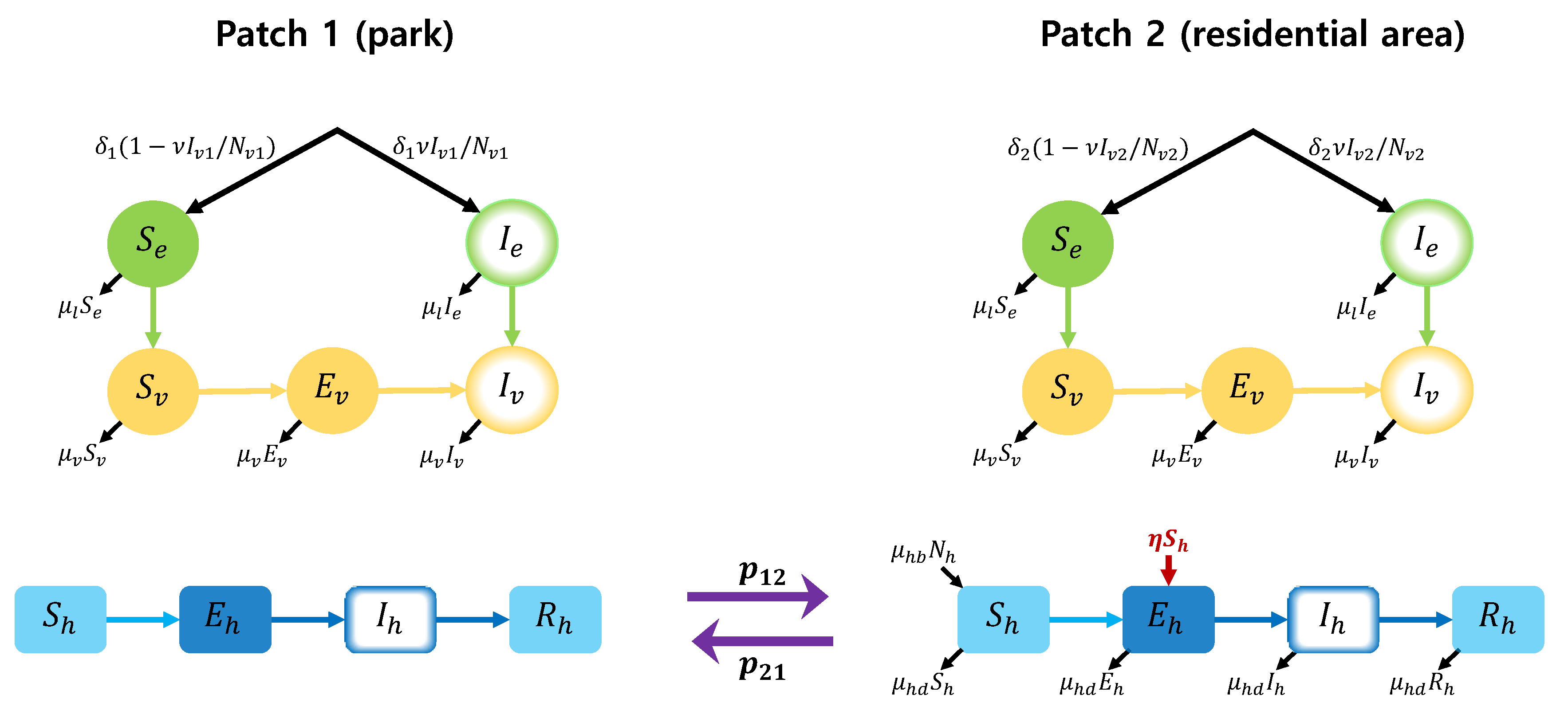
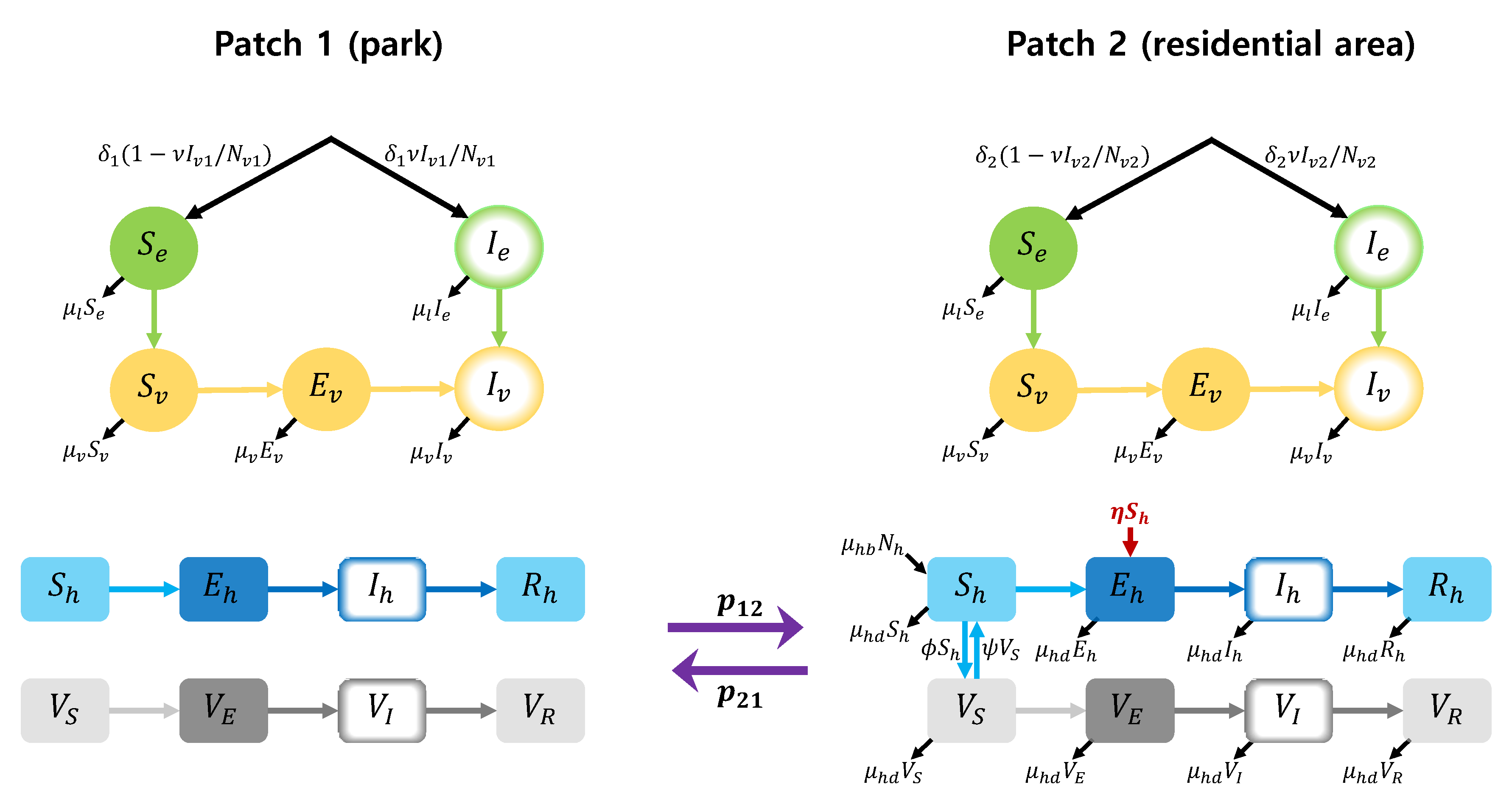
In this section, we develop a two-patch dengue transmission model by applying differential equation approach. It is assumed that patch 1 is a park area where mosquitoes prevail, and patch 2 is a residential area where people live. The focus area for the model is Seoul Forest Park (patch 1) and the residential area (patch 2) around the park in Seoul, Korea. A schematic diagram of the full two-patch model is shown in Figure 1. The model considers the states of mosquito larvae (susceptible () and infectious () by vertical infection), female adult mosquitoes (susceptible (), exposed () and infectious ()) and humans (susceptible (), exposed (), infectious () and recovered ()), for patch . We denote the total larvae population, female adult mosquito population and human population by , and for patch . That is, , and . To describe the transmission dynamics in patch 2, we use the dengue model in [14]. In our two-patch model, we assume that humans can move between patches, but mosquitoes cannot.
We write the governing equations of the model as follows:
In the governing Equation (1), the parameters relevant to larvae and mosquitoes are described as follows: is the maturation rate of pre-adult mosquitoes, and and are the mortality rate of adult mosquitoes and larvae, respectively. and denote the rate of vertical infection from infected mosquitoes to eggs and the extrinsic incubation period, respectively, and is the number of new recruits in the larva stage for patch . The parameters and are the transmissible rates from mosquito to human and from human to mosquito, respectively, where b is the daily biting rate of a mosquito and and are the probability of infection from human to mosquito per bite and the probability of infection from mosquito to human per bite, respectively [14]. The parameters and represent the human birth rate and death rate, respectively, and the two rates are assumed to be equal. The parameters and are the latent period and infectious period for humans, respectively. The inflow rate of infection due to international travelers is defined by [14]. refers to the human movement rate from patch i to j, where and for . Since there are about 7,500,000 visitors to Seoul Forest Park each year [15], approximately 20,550 people visit the park daily. Hence, assuming , i.e., the total human population of both patches is , we compute . Moreover, we assume that , which represents that a small number of people such as park keepers and homeless people stay in the park, and .
2.2. Parameter Estimation
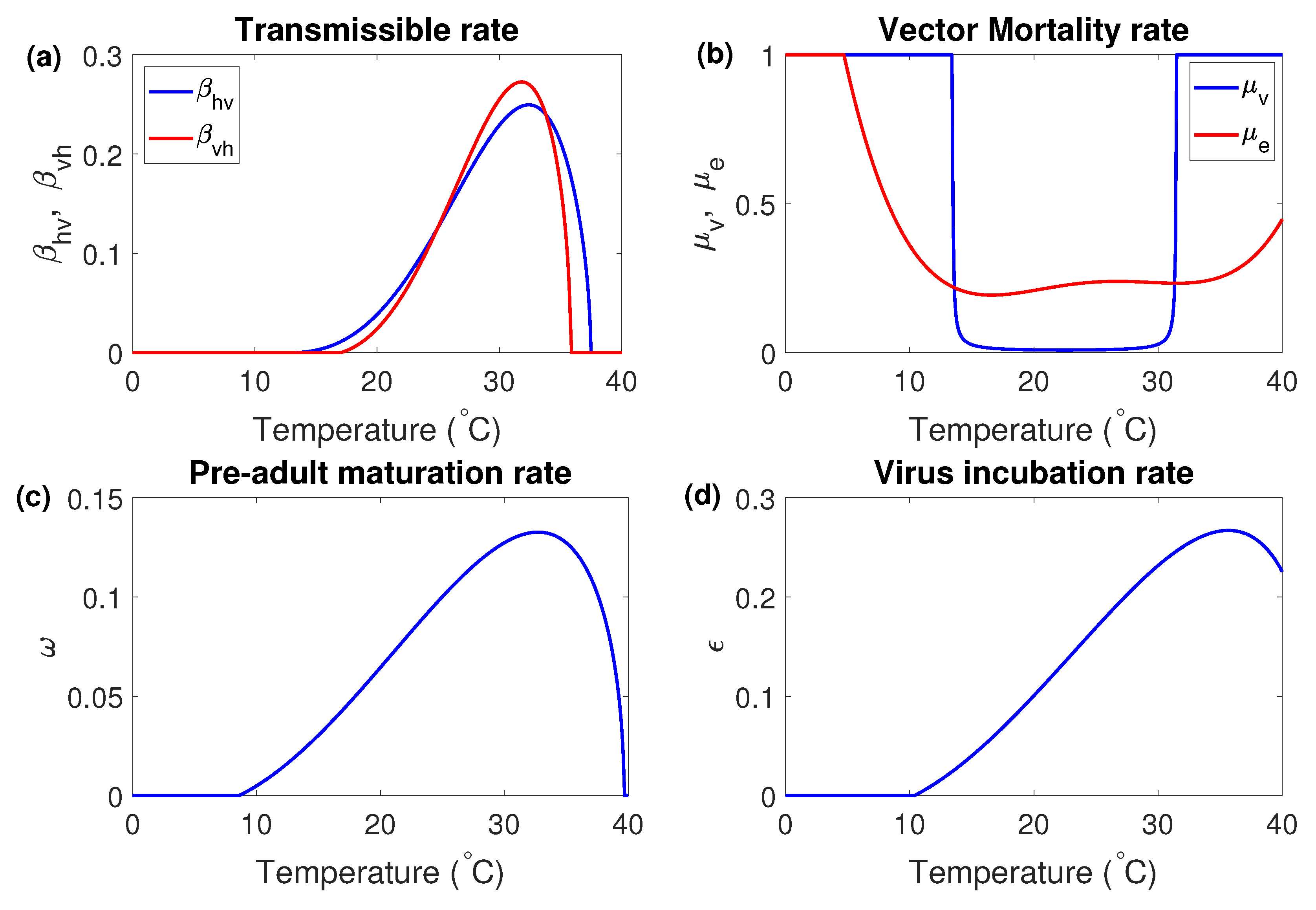
The temperature-sensitive parameters for the dengue mosquitoes have been studied in previous researches [14,16,21,22,23,24,25]. Using the previous results, we describe the parameters sensitive to the temperature as the following temperature-dependent functions.
- (1)
- (2)
- The probability of infection from mosquito to human per bite is [21]
- (3)
- The probability of infection from human to mosquito per bite is [21]
- (4)
- The mortality rate of the adult mosquito is [21]
- (5)
- Pre-adult maturation rate is [21]
- (6)
- Virus incubation rate is [21]
- (7)
- The mortality rate of larva (aquatic phase mortality rate) is [24]
- (8)
- The number of new recruits in the larvae stage for patch is computed as [14]
Figure 2 illustrates the the graph of the temperature-dependent parameters.
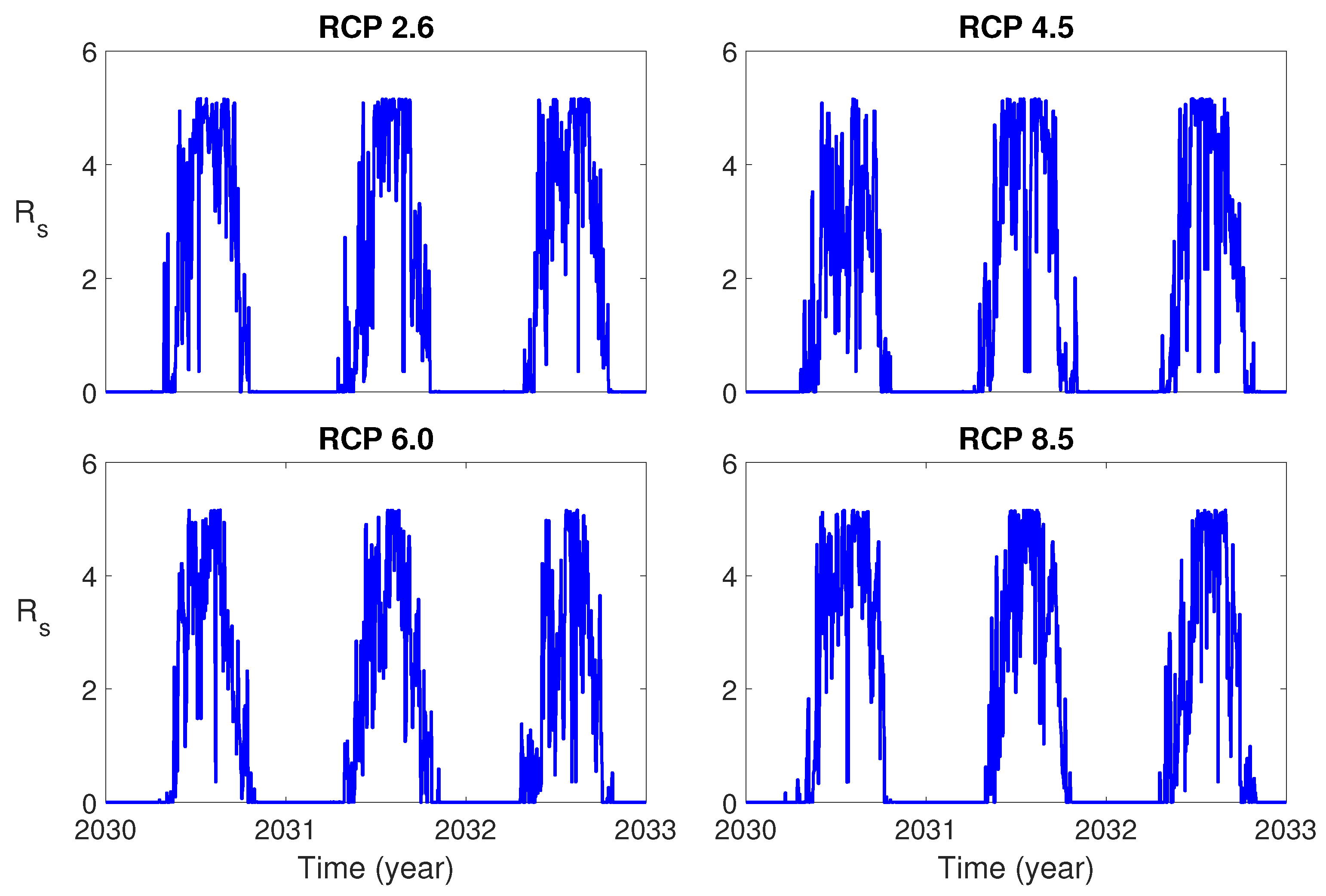
For the temperature data, we utilize RCP scenarios, which provide four representative scenarios such as the low level scenario (RCP 2.6), the two medium level scenarios (RCP 4.5/6.0) and the high level scenario (RCP 8.5) [27]. Since patch 1, Seoul Forest Park, is located in Seongdong-gu, Seoul, the RCP temperature data for Seongdong-gu is used in the simulation. One can see the tendency of the temperature rise between 2030 and 2100 according to the RCP scenarios (refer to Appendix A).
2.3. The Seasonal Reproduction Number
The basic reproduction number is important in epidemiology since it measures the expected number of infectious cases directly caused by one infectious case in a susceptible population. It is known that if , the system has a locally asymptotically stable disease-free equilibrium, but if , it has an unstable disease-free equilibrium [28]. However, when some model parameters are time-dependent as in Table 1, one has to use the seasonal reproduction number instead of the basic reproduction number [29].
Theorem 1.
The seasonal reproduction number corresponding to a single patch model with only patch 2 without the inflow rate η is computed as
Proof.
The proof of the theorem can be found in Appendix B. ☐
Theorem 2.
The seasonal reproduction number in the two-patch model (1) is the spectral radius ρ of the matrix G, i.e.,
where
and
Proof.
The proof of the theorem can be found in Appendix B. ☐
Figure 3 shows the seasonal reproduction number for three years from 1 January 2030 for each RCP scenario. It is observed that the value of is much higher than 1 in the summer season for all RCP scenarios. This implies that it is very likely that the dengue outbreak will occur during the summer.
3. Results
3.1. Dengue Transmission Dynamics Based on Rcp Scenarios
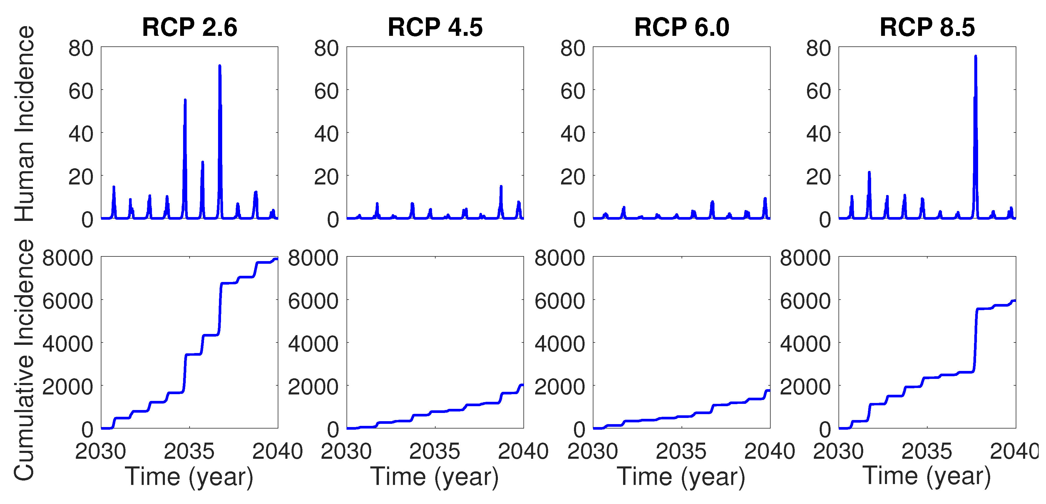
In this section, we perform numerical simulations for the two patch model based on RCP scenarios. For each simulation, we assume the initial condition as where . Moreover, we assume that there are no infected mosquitoes and humans initially, that is, and for , so that the first infection in the model is initiated by the inflow of infected international travelers. Figure 4 shows the time evolution of human incidence and cumulative human incidence from January 1 in 2030 for 10 years in the model without control for each RCP scenario. One can see that there will be more dengue incidences for RCP 2.6 and 8.5 than RCP 4.5 and 6.0, which implies that the two extreme level RCP scenarios might provide more favorable temperature environment for dengue virus transmission than the two medium level RCP scenarios.
3.2. The Effects of Human and Vector Controls
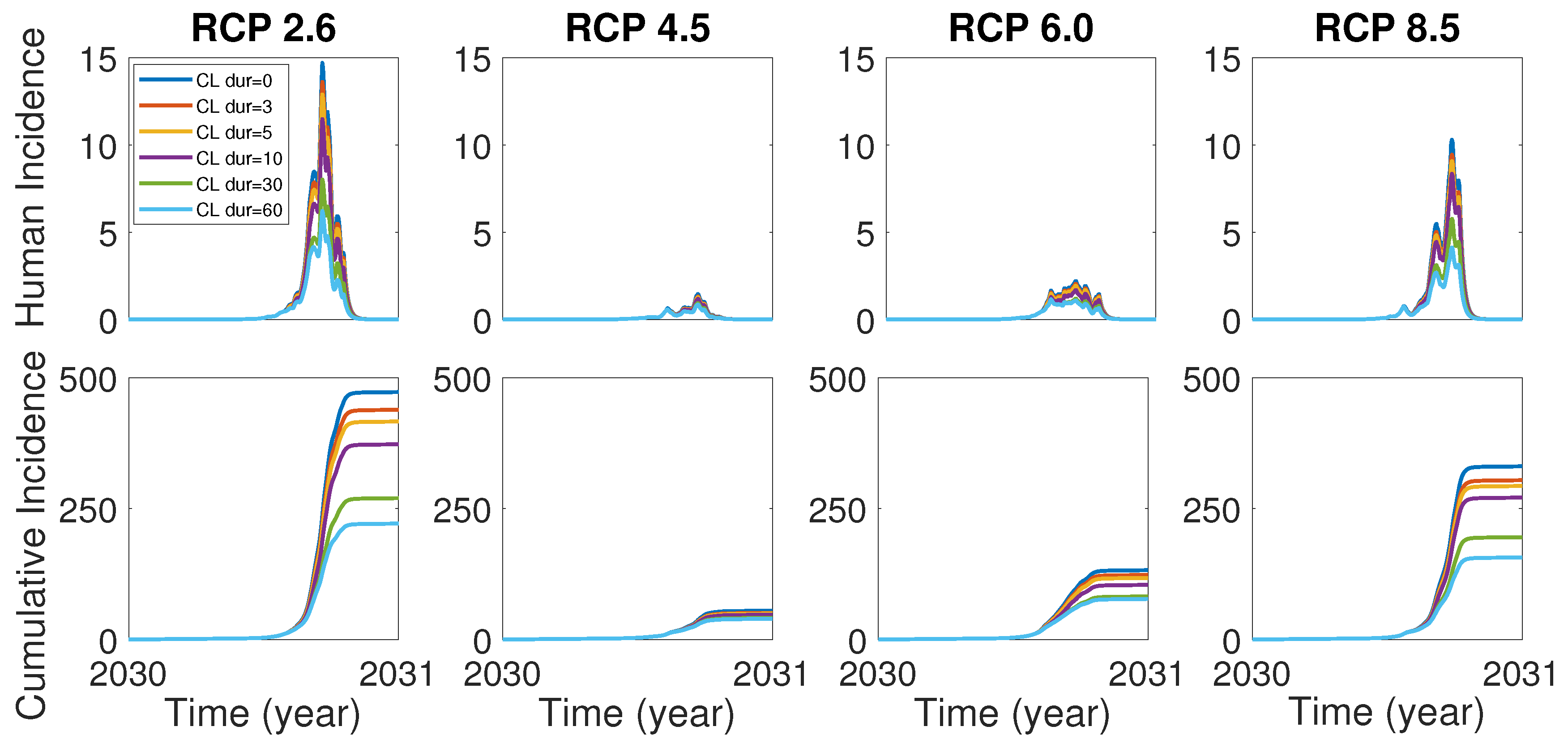
In the case of the dengue outbreak in Tokyo, Yoyogi park in the city was known as an infection hub and the closure of the park turned out to be very effective control strategies [8]. In accordance with the case in Tokyo, it is worth investigating the effects of the control strategies including the park closure as well as vector and human controls for our model (1). We assume that the park closure begins when the cumulative incidence is over 10. In order to see the control effect of the park closure, we set , and all human population stays in the city area (patch 2). Figure 5 shows the effect of park closure for duration 3, 5, 10, 30, 60 days. It is observed that the park closure for a short-term period such as 3 and 5 days would be effective in a certain degree and the closure for a long-term period such as 30 and 60 days would make a significant control effect for all RCP scenarios.
Concerning the control for mosquitoes and humans, it was estimated that the current level of control for mosquitoes in Korea is about increase of mosquito death rate and decrease of transmissible rate between mosquitoes and humans, respectively, and these control measures were implemented between May and October in each year [29].
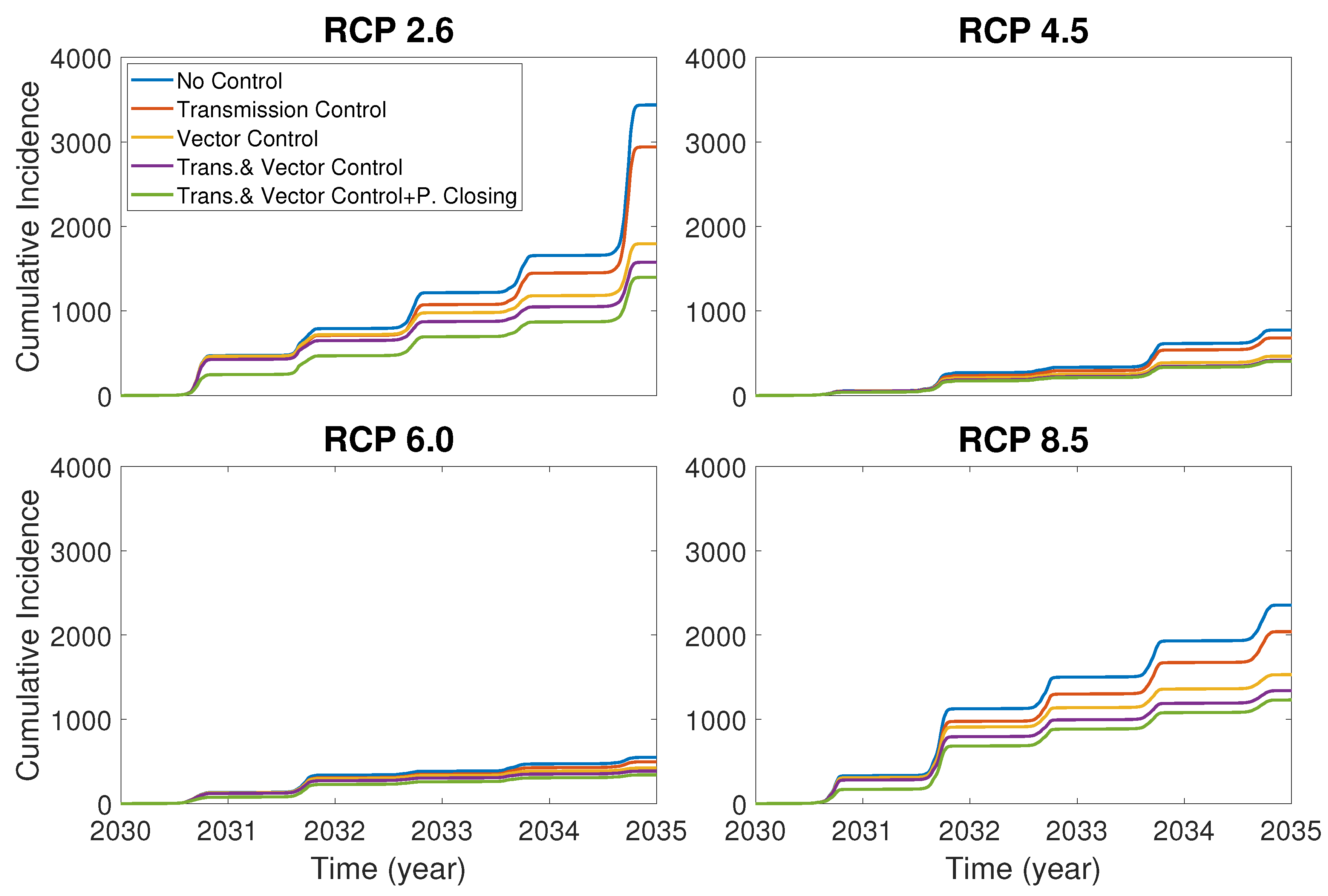
Now we compare the control effects of the vector death rate, dengue transmissible rate and park closure. In Figure 6, it is assumed that the controls of the vector death rate and dengue transmissible rate are implemented as a increase and a decrease of the rates, respectively, and the park closure is made for only 30 days in the year 2030 at the early stage of the dengue outbreak. Figure 6 shows that the vector control is more effective than the transmission control, and the combination of the park closure and vector and human control is most effective.
3.3. Optimal Control
In this section, we implement effective control measures by formulating an optimal control problem for the two-patch dengue model. By incorporating the control functions and into the transmissible rate between the vector and human and the mortality rate of the vector in each patch, respectively, in the model Equation (1), we obtain the controlled two-patch system (2) as follows:
Now we set up an optimal control problem for the two-patch model in order to minimize the proportions of infected vectors and humans in both patches for a finite time interval at a minimal cost of implementation. We first define the classical objective functional [30,31]
where and denote the weight constants on the infected humans and vectors and the total vectors, respectively, and and denote the weight constants that are the relative costs of the implementation of the preventive controls for decreasing the transmissible rate between vector and human and increasing the mortality rate of the vector, respectively.
Then, we find an optimal solution that satisfies
where subject to the state equations with and . It is known that the standard results of optimal control theory guarantees the existence of optimal controls, and the necessary conditions of optimal solutions can be derived from Pontryagin maximum principle [31,32]. The Pontryagin maximum principle converts the system (2) into the problem of minimizing the Hamiltonian given by
Using the Hamiltonian H and the Pontryagin maximum principle, we obtain the theorem.
Theorem 3.
There exist optimal controls and state solutions which minimize over Ω in (3). In order for the above statement to be true, it is necessary that there exist continuous functions such that
with the transversality conditions for and the optimality conditions
Proof.
The proof of the theorem can be found in Appendix B. ☐
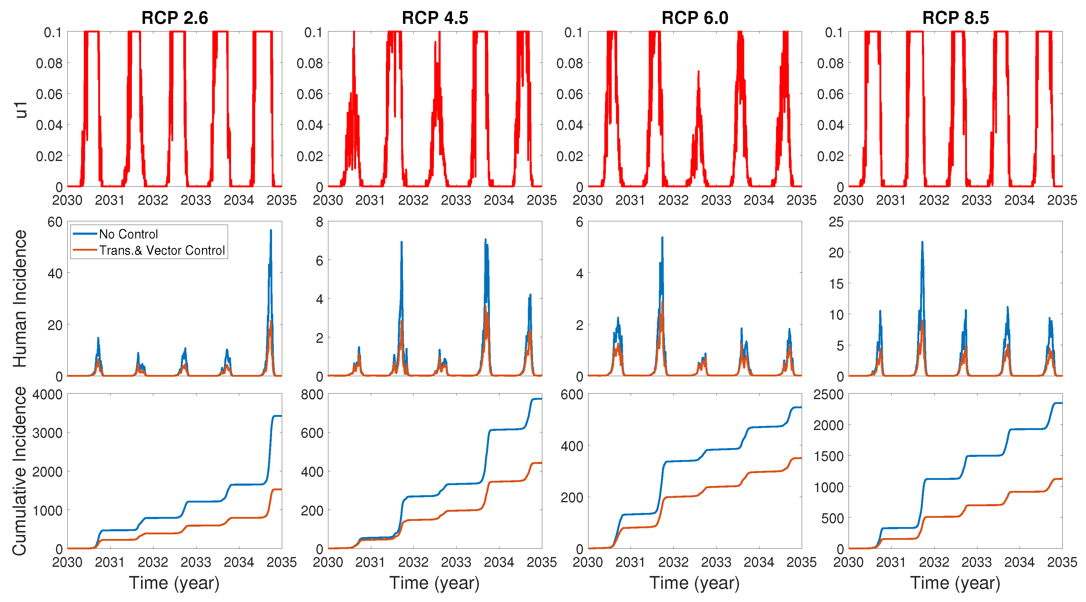
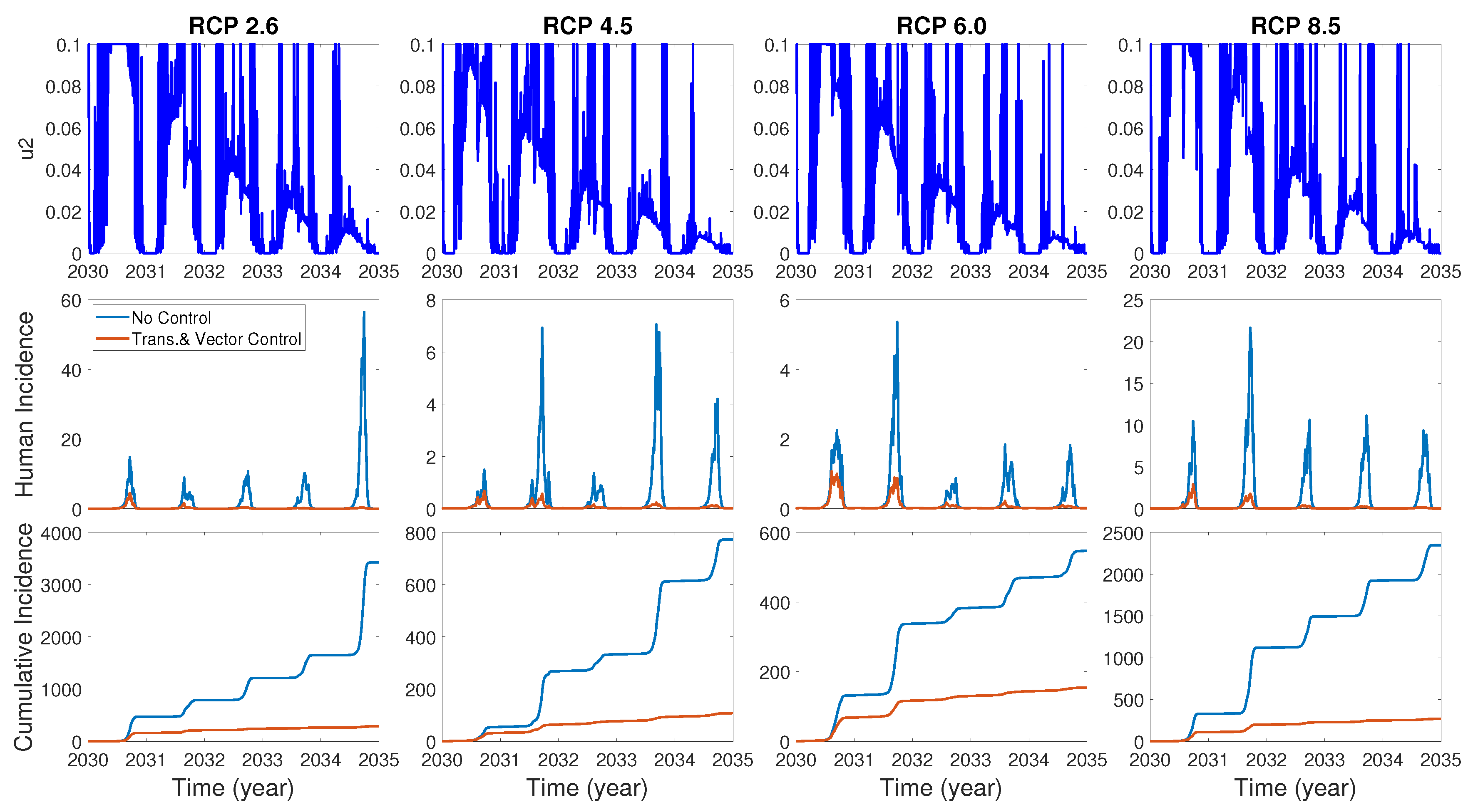
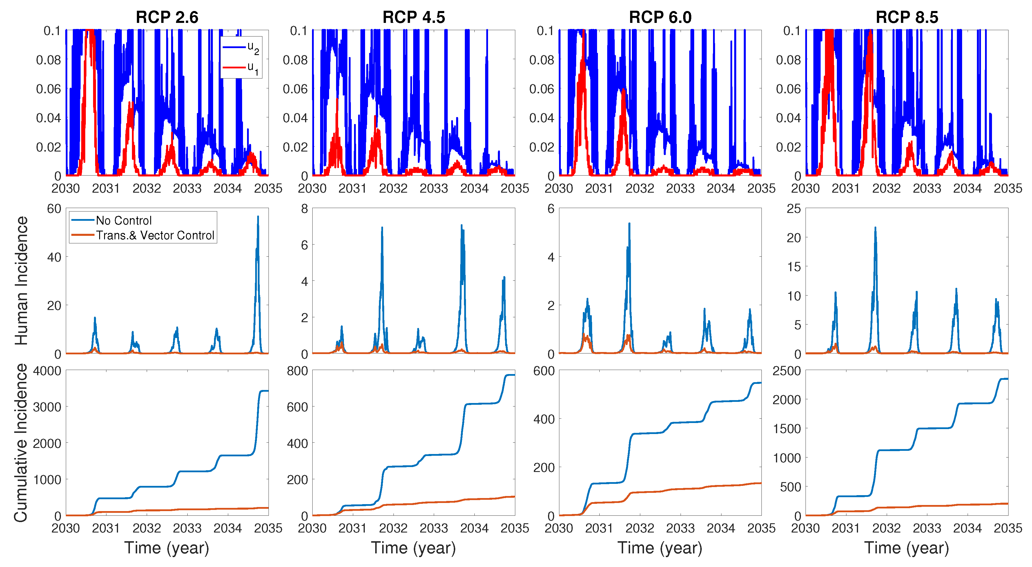
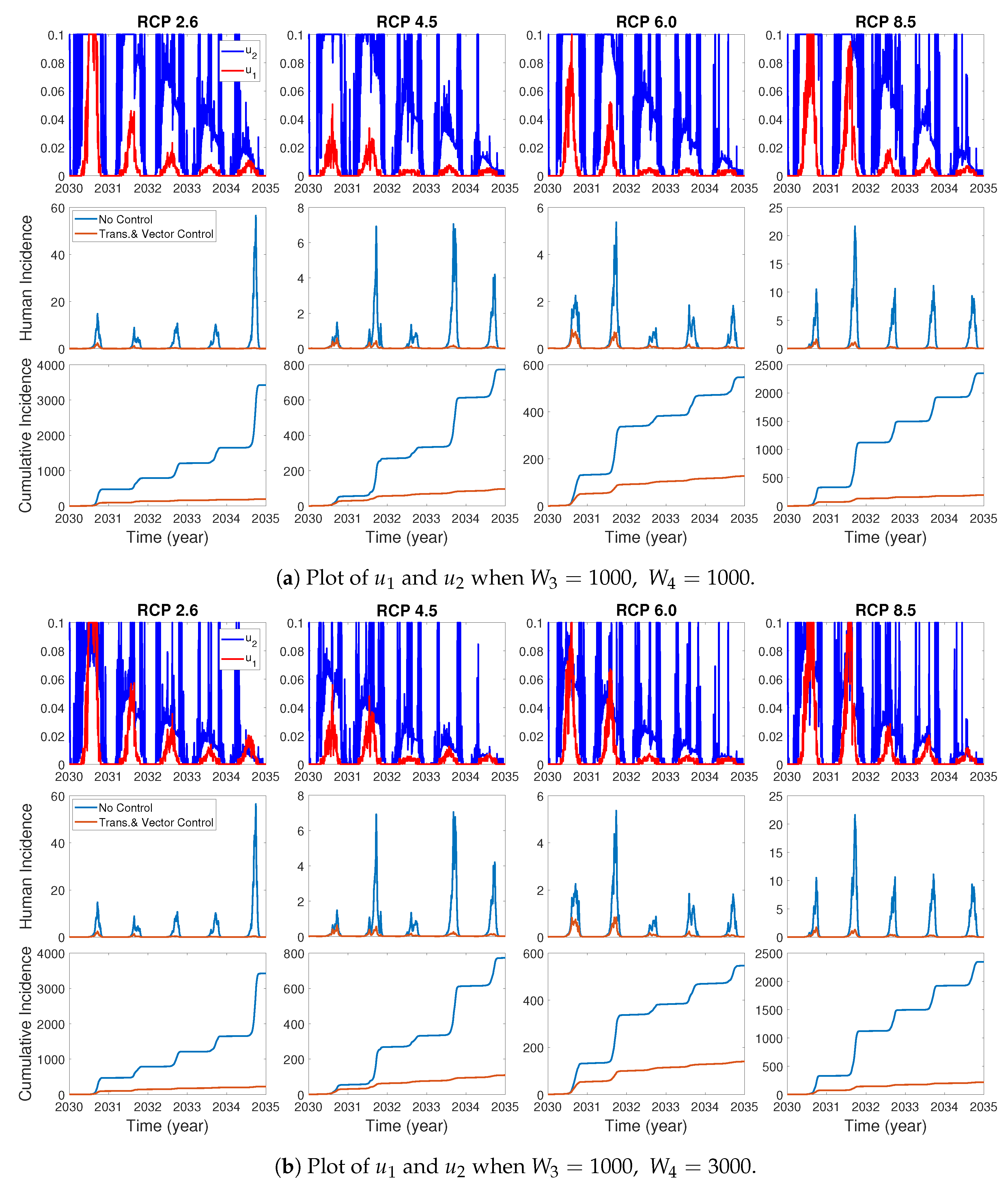
We assume the control duration as 5 years throughout the simulations, and the upper bound for is 0.1, since the control resources are limited. In Figure 7, Figure 8 and Figure 9, we simulate the effects on incidence and optimal control functions from different control strategies when only the transmissible rates are controlled, only the mortality rate is controlled and both the transmissible rates and the mortality rate are controlled, respectively. Considering the ratio of the number of infected vectors and humans to the total number of vectors, we use the weight constants , , and for Figure 7, Figure 8 and Figure 9. Figure 7 suggests that when the transmission control is considered, it is effective to focus on the control during the summer. Moreover, Figure 8 shows that the peaks of occasionally occurred, and Figure 9 implies that when all , and are controlled, the control period of is longer than and . These results imply that it is more effective if the controls are concentrated right before the summer outbreak, since seasonal patterns are observed in all cases. For more cases with different weight constants, refer to Appendix C.
3.4. Vaccination Model and Cost-Effectiveness of Control Strategies
Recently the vaccine for dengue such as Dengvaxia has been used to prevent dengue transmission in the dengue-endemic countries including Mexico, Philippines, Indonesia and Brazil [33]. A recent research investigated the cost-effectiveness of dengue vaccination in Mexico [20], which concluded that a proper dengue vaccination program would be very cost-effective and also highly reduce the dengue cases and casualties. Thus, it is worth investigating the cost-effectiveness of control strategies including vaccination in our two-patch model. We assume that the vaccination will begin at the year 2030 and any susceptible individual, either seropositive or seronegative, can be vaccinated.
In order to consider the effect of the vaccination, we first construct a two-patch dengue transmission model with vaccination by modifying the model (1). The model with vaccination includes the new compartments such as and which denote the vaccinated susceptible, exposed, infected and recovered human class in patch , respectively. The schematic diagram for the model is shown in Figure 10.
The governing equation for the model is written as follows:
where the parameter denotes the rate at which vaccine wanes off and the vaccination rate followed by antibody formation is computed by , where a is the proportion of the vaccinated humans and b is the vaccination period. Here, we assume and days between June and September. The parameters relevant to vaccination are described in Table 2.
We evaluate the cost-effectiveness of the control measures such as vector control, dengue virus transmission control, and vaccination by using the incremental cost-effectiveness ratio (ICER) in terms of dollars per quality-adjusted life year (QALY) gained for a range of control costs. The cost-effectiveness of a control strategy is related to the costs per disability-adjusted life years (DALY) and gross domestic product (GDP) per capita; (i) a control strategy is very cost-effective if the costs per DALY are less than GDP per capita, (ii) cost-effective if the costs per DALY are between GDP per capita and GDP per capita and (iii) not cost-effective if the costs per DALY are greater than GDP per capita [20,36]. The QALY function Q is computed as follows [20,37]:
where D is the disability weight for dengue fever(DF), dengue hemorrhagic fever(DHF) and death, which are denoted by , and , respectively, C is the age-weighting correction constant, h is the parameter from the age-weighting function, a is the average age, L is the duration of the disability or the years of life lost due to premature death expressed in years such as , or and r is the social discount rate [37]. The total QALYs lost (TQL) is computed as follows [20]:
where the rates of new DF, DHF and death cases for the vector and transmission control are
and the rates for the vaccination case are
The total cost is obtained by the sum of the cost for direct control along the control strategies and the cost associated with dengue infection under the observation period . The direct controls we consider are vector control, transmission control and vaccination where the costs of each direct control are , and , respectively. The costs associated with dengue infection DF and DHF are and , respectively, where each cost is estimated from [20]. The total cost (TC) for each control strategy is computed as follows:
(i) Total costs for vector control:
(ii) Total costs for transmissible rate control:
(iii) Total costs for vaccination:
The parameters relevant to cost-effectiveness are described in Table 3.
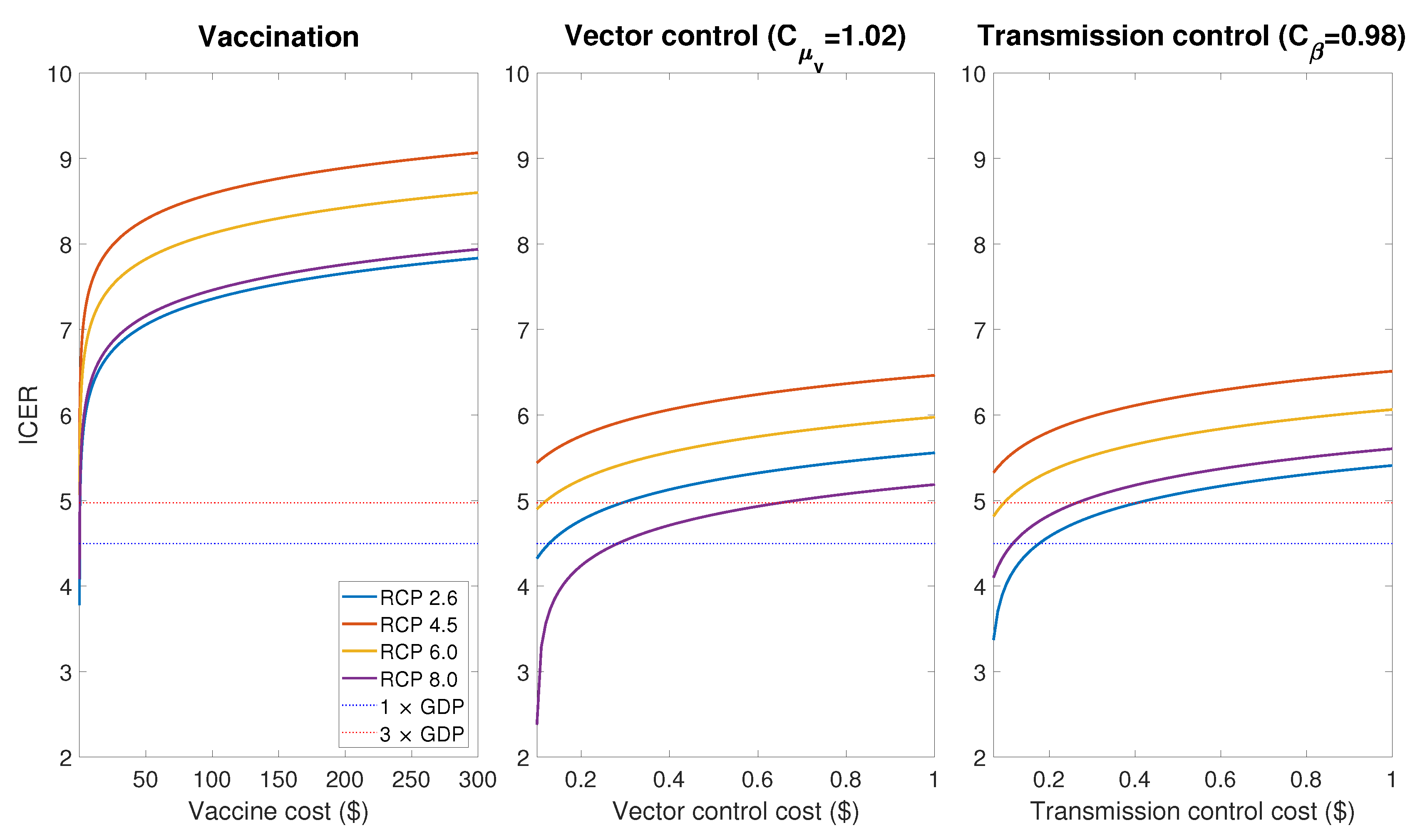
In order to evaluate the cost-effectiveness of controls, we use the incremental cost-effectiveness ratio (ICER) which is calculated by dividing the difference in total costs (incremental cost) by the difference in the QALY with and without control cases. Figure 11 shows ICER per DALY averted for the vaccination, vector control and transmission control cases. Here we assume, as in Section 3.2, that the vector control and transmission control are implemented as a increase of mosquito death rate and a decrease of transmissible rate between May and October, respectively. According to recent researches, it was estimated that the cost of vaccination per capita is hundreds of USD [20,43], while the cost per capita of the vector control and the transmission control ranges from tens of cents to a few dollars in USD [44,45]. Thus, the results of Figure 11 imply that vector control and transmission control are relatively more cost-effective than vaccination, and vaccination is not a suitable control strategy in Korea in terms of cost-effectiveness.
4. Discussion and Conclusions
In this paper, we developed the two-patch dengue transmission model associated with temperature-dependent parameters. The focus area for the model was Seoul Forest Park (patch 1) and the residential area (patch 2) around the park in Seoul, the most populated city in Korea. In the model, we represented the parameters sensitive to temperature as the temperature-dependent nonlinear functions using the previous literatures. Using the temperature data under RCP climate change scenarios, we investigated the dengue transmission dynamics within and between patches. The simulation results for the model showed that if a dengue infection is initiated by the inflow of infected international travelers into the focus area, there will be thousands of infected humans within 10 years in the case of no controls for the dengue disease.
We derived the formulas for the seasonal reproduction number for the single-patch (patch 2) and the two-patch model by using the next generation matrix. The simulation results (Figure 3) for showed that the value of is much bigger than 1 in the summer season for all RCP scenarios. This implies that it is very likely that the dengue outbreak will occur during the summer in the near future, if there is no proper control strategy. To reduce the potential of the dengue outbreak, proper control strategies should be implemented.
We studied optimal control strategies by using an optimal control framework under different scenarios. We found that the control strategies are effective if they are implemented right before the summer outbreak. Concerning the park closure, we found that the closure for a short-term period such as 3 and 5 days would be effective in a certain degree, but the closure for a long-term period such as 30 and 60 days would make a substantial control effect.
By incorporating the vaccination policy into the two-patch model, we constructed the two-patch dengue transmission model (5) with vaccination. Concerning the vaccination, currently Dengvaxia is vaccinated for seropositive cases and also other vaccines are now in clinical development [46,47]. Since our model simulation begins at the year 2030, there is a possibility of the development of other vaccines which can be used for any susceptible cases, either seropositive or seronegative. In light of this aspect, in the vaccination model (5), we assume that any susceptible individual, seropositive or seronegative, can be vaccinated. We investigated the cost-effectiveness of the control policies such as vaccination, vector control, and transmission control, using the incremental cost-effectiveness ratio (ICER) in terms of dollars per quality-adjusted life year (QALY). We found that the transmissible rate control and the vector control are cost-effective while the vaccination is less cost-effective. This result is not compatible with the result in Mexico [20] because there are not a sufficient number of infective humans in Korea, compared to the case of Mexico.
Since there have been no autochthonous dengue cases in Korea yet, the parameters relevant to the cost of the dengue vaccination were adapted from the previous studies in dengue-endemic regions [20,39,40]. Moreover, to the best of our knowledge, there have been no studies about the relation between the cost and effectiveness of the dengue control in Korea. Although these factors may result in a limitation in the accurate estimation of the cost-effectiveness for the control strategies, the simulation results (Figure 11) clearly show the difference in cost-effectiveness between different strategies; when the control resources are limited, it is more effective to implement vector control and transmission control rather than vaccination.
In this research, we used the regional data such as temperature and human movement rate for Seoul, Korea. Thus, most of the results presented in this paper may not be applied directly to the area with different environment for mosquitoes and humans, but we expect that the modeling approach presented in this work will be applied to other cases, especially when the temperature-dependent transmission dynamics between endemic and non-endemic regions are investigated.
Author Contributions
Conceptualization, J.E.K., S.L. and C.H.L.; methodology, J.E.K., Y.C. and C.H.L.; software, J.E.K. and Y.C.; validation, J.E.K., Y.C., J.S.K., S.L. and C.H.L.; formal analysis, J.E.K., Y.C. and C.H.L.; investigation, J.E.K., Y.C., J.S.K. and C.H.L.; data curation, J.E.K. and Y.C.; writing—original draft preparation, J.E.K., Y.C. and C.H.L.; writing—review and editing, J.S.K., S.L. and C.H.L.; visualization, J.E.K. and Y.C.; supervision, S.L. and C.H.L.; All authors have read and agreed to the published version of the manuscript.
Funding
J.E.K. was supported by Basic Science Research Program through the National Research Foundation of Korea (NRF) funded by the Ministry of Education (2018R1D1A1B07047163). C.H.L. was supported by the National Research Foundation of Korea(NRF) grant funded by the Korea government(MSIT)(2019R1F1A1040756). S.L. was supported by a National Research Foundation of Korea (NRF) grant funded by the Korean government (MSIP) (NRF-2018R1A2B6007668).
Conflicts of Interest
The authors declare no conflict of interest. The funders had no role in the design of the study; in the collection, analyses, or interpretation of data; in the writing of the manuscript, or in the decision to publish the results.
Appendix A. Temperature Data under RCP Scenarios
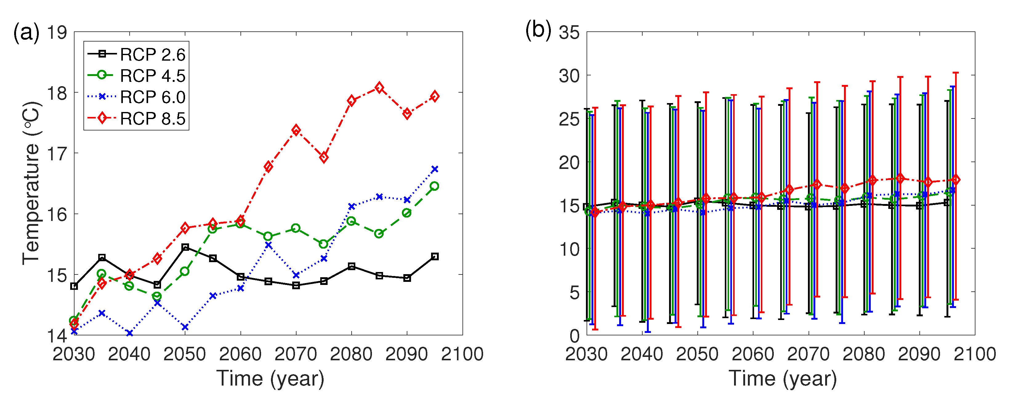
The Intergovernmental Panel on Climate Change has developed RCP scenarios in 2014, and four representative scenarios are the lowest-level scenario (RCP 2.6), the two medium level scenarios (RCP 4.5/6.0) and the high-level scenario (RCP 8.5) [27]. In this paper, we use the daily climate data estimated by the Korea Meteorological Administration under the four RCP scenarios. Figure A1 illustrates the 5-year averages of daily temperature and the ranges from the mean temperature in the summer (June to August) to the mean temperature in the winter (December to February) for five years in Seongdong-gu, Seoul from year 2030 to 2099.
Figure A1.
(a) Daily mean temperature for five years. (b) Range from the mean temperature in the summer (June to August) to the mean temperature in the winter (December to February) for five years.
Figure A1.
(a) Daily mean temperature for five years. (b) Range from the mean temperature in the summer (June to August) to the mean temperature in the winter (December to February) for five years.

Appendix B. Proofs of Theorems 1, 2 and 3
Proof of Theorem 1.
The system for the single-patch model with only patch 2 has the disease-free state with . Let ,
and
Here denotes all of the new infections and denotes the net transition rates of the corresponding compartment. F and V are 5 × 5 matrices at given by
Hence, the next generation matrix G is computed as
Since the seasonal reproduction number for the single-patch model is the dominant eigenvalue of the matrix G, is obtained as
☐
Proof of Theorem 2.
The system (1) has the disease-free state with . Let for . If and denote the functions for all of the new infections and the net transition rates of the corresponding compartment, respectively, then one can obtain
and
Thus, F and V are 10 × 10 matrices at given by
and
Hence, one can obtain the next generation matrix G as
where
and
Finally, the seasonal reproduction number for the two-patch model is computed as the spectral radius of the next generation matrix G, i.e., . ☐
Proof of Theorem 3.
Since the integrand of J is a convex function of and the state system satisfies the Lipschitz condition, the existence of the optimal controls can be proved by Corollary 4.1 of [32]. Moreover, using the system (5) and the Pontryagin Maximum Principle, one can obtain the following:
with for and evaluating the above system at the optimal controls and corresponding states, one can obtain the adjoint system. Since the Hamiltonian is minimized with respect to the controls, we differentiate with respect to on the set , and obtain the following optimality conditions:
Solving for , one can obtain
By using the standard argument for bounds for , we have the optimality conditions. ☐
Appendix C. Optimal Control Result with Different Weight Constants
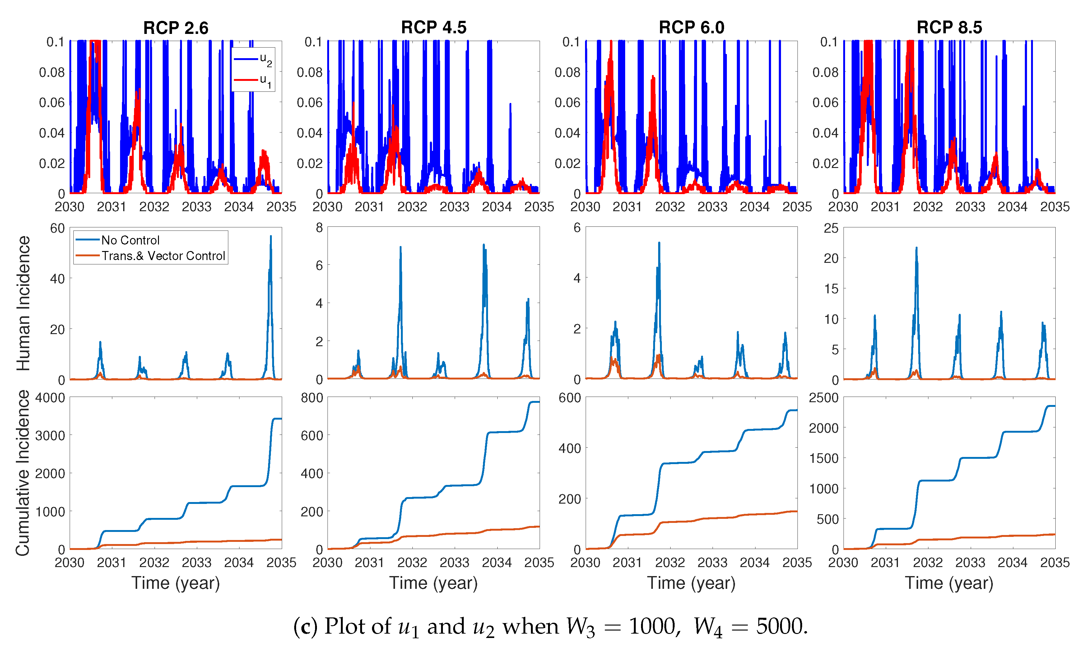
We consider various weight constants for the case that all of , and are controlled. Figure A2a–c show the plots of and for , when are fixed. One can see the similar results as in Section 3.3.
Figure A2.
The effect of different weight constant values on the optimal control functions.


References
- Cook, G.C.; Zumla, A. Manson’s Tropical Diseases; Elsevier Health Sciences: Amsterdam, The Netherlands, 2008. [Google Scholar]
- Martens, P. Health and Climate Change: Modelling the Impacts of Global Warming and Ozone Depletion; Routledge: Abingdon-on-Thames, UK, 2013. [Google Scholar]
- Teixeira, M.G.; Siqueira, J.B.; Germano, L., Jr.; Bricks, L.; Joint, G. Epidemiological trends of dengue disease in brazil (2000–2010): A systematic literature search and analysis. PLoS Negl. Trop. Dis. 2013, 7, e2520. [Google Scholar] [CrossRef] [PubMed] [Green Version]
- Morin, C.W.; Comrie, A.C.; Ernst, K. Climate and dengue transmission: Evidence and implications. Environ. Health Perspect. 2013, 121, 1264–1272. [Google Scholar] [CrossRef] [PubMed]
- Naish, S.; Dale, P.; Mackenzie, J.S.; McBride, J.; Mengersen, K.; Tong, S. Climate change and dengue: A critical and systematic review of quantitative modelling approaches. BMC Infect. Dis. 2014, 14, 167. [Google Scholar] [CrossRef] [Green Version]
- Liu-Helmersson, J.; Stenlund, H.; Wilder-Smith, A.; Rocklöv, J. Vectorial capacity of aedes aegypti: Effects of temperature and implications for global dengue epidemic potential. PLoS ONE 2014, 9, e89783. [Google Scholar] [CrossRef] [Green Version]
- Chen, S.-C.; Hsieh, M.-H. Modeling the transmission dynamics of dengue fever: Implications of temperature effects. Sci. Total Environ. 2012, 431, 385–391. [Google Scholar] [CrossRef] [PubMed]
- Kutsuna, S.; Kato, Y.; Moi, M.L.; Kotaki, A.; Ota, M.; Shinohara, K.; Kobayashi, T.; Yamamoto, K.; Fujiya, Y.; Mawatari, M.; et al. Autochthonous dengue fever, Tokyo, Japan, 2014. Emerg. Infect. Dis. 2015, 21, 517. [Google Scholar] [CrossRef] [Green Version]
- Yuan, B.; Lee, H.; Nishiura, H. Assessing dengue control in Tokyo, 2014. PLoS Negl. Trop. Dis. 2019, 13, e0007468. [Google Scholar] [CrossRef] [Green Version]
- Cho, H.-W.; Chu, C. A disease around the corner. Osong Public Health Res. Perspect. 2016, 7, 1–2. [Google Scholar] [CrossRef] [Green Version]
- Jeong, Y.E.; Lee, W.-C.; Cho, J.E.; Han, M.-G.; Lee, W.-J. Comparison of the epidemiological aspects of imported dengue cases between korea and japan, 2006–2010. Osong Public Health Res. Perspect. 2016, 7, 71–74. [Google Scholar] [CrossRef] [Green Version]
- Lim, S.-K.; Lee, Y.S.; Namkung, S.; Lim, J.K.; Yoon, I.-K. Prospects for dengue vaccines for travelers. Clin. Exp. Vaccine Res. 2016, 5, 89–100. [Google Scholar] [CrossRef] [Green Version]
- Lee, J.-S.; Farlow, A. The threat of climate change to non-dengue-endemic countries: Increasing risk of dengue transmission potential using climate and non-climate datasets. BMC Public Health 2019, 19, 934. [Google Scholar] [CrossRef] [PubMed]
- Lee, H.; Kim, J.E.; Lee, S.; Lee, C.H. Potential effects of climate change on dengue transmission dynamics in Korea. PLoS ONE 2018, 13, e0199205. [Google Scholar] [CrossRef]
- Landscape Architecture Korea (LAK). 2019. Available online: https://www.lak.co.kr/m/news/view.php?id=7248 (accessed on 20 June 2020).
- Adams, B.; Boots, M. How important is vertical transmission in mosquitoes for the persistence of dengue? insights from a mathematical model. Epidemics 2010, 2, 1–10. [Google Scholar] [CrossRef]
- Wearing, H.J.; Rohani, P. Ecological and immunological determinants of dengue epidemics. Proc. Natl. Acad. Sci. USA 2016, 103, 11802–11807. [Google Scholar] [CrossRef] [PubMed] [Green Version]
- Janreung, S.; Chinviriyasit, W. Dengue fever with two strains in thailand. Int. J. Appl. Phys. Math. 2014, 4, 55. [Google Scholar]
- Korean Statistical Information Service(KOSIS), Population Projections and Summary Indicators (Province). 2017. Available online: http://kosis.kr/eng/ (accessed on 29 May 2020).
- Shim, E. Cost-effectiveness of dengue vaccination in yucatán, mexico using a dynamic dengue transmission model. PLoS ONE 2017, 12, e0175020. [Google Scholar] [CrossRef]
- Mordecai, E.A.; Cohen, J.M.; Evans, M.V.; Gudapati, P.; Johnson, L.R.; Lippi, C.A.; Miazgowicz, K.; Murdock, C.C.; Rohr, J.R.; Ryan, S.J.; et al. Detecting the impact of temperature on transmission of zika, dengue, and chikungunya using mechanistic models. PLoS Negl. Trop. Dis. 2017, 11, e0005568. [Google Scholar] [CrossRef] [PubMed] [Green Version]
- Derouich, M.; Boutayeb, A.; Twizell, E. A model of dengue fever. BioMed. Eng. OnLine 2003, 2, 1. [Google Scholar] [CrossRef] [PubMed] [Green Version]
- Tran, A.; L’Ambert, G.; Lacour, G.; Benoît, R.; Demarchi, M.; Cros, M.; Cailly, P.; Aubry-Kientz, M.; Balenghien, T.; Ezanno, P. A rainfall-and temperature-driven abundance model for aedes albopictus populations. Int. J. Environ. Res. Public Health 2013, 10, 1698–1719. [Google Scholar] [CrossRef] [Green Version]
- Yang, H.; Macoris, M.d.L.d.G.; Galvani, K.; Andrighetti, M.; Wanderley, D. Assessing the effects of temperature on the population of aedes aegypti, the vector of dengue. Epidemiol. Infect. 2009, 137, 1188–1202. [Google Scholar] [CrossRef] [Green Version]
- Tjaden, N.B.; Thomas, S.M.; Fischer, D.; Beierkuhnlein, C. Extrinsic incubation period of dengue: Knowledge, backlog, and applications of temperature dependence. PLoS Negl. Trop. Dis. 2013, 7, e2207. [Google Scholar] [CrossRef] [PubMed] [Green Version]
- Korea Centers for Disease Control and Prevention (KCDC), Mathematical Modelling on p.vivax Malaria Transmission and Development of Its Application Program. 2009. Available online: http://www.cdc.go.kr/cdc_eng/ (accessed on 29 May 2020).
- Intergovernmental Panel on Climate Change (IPCC), Fifth Assessment Report. 2014. Available online: https://www.ipcc.ch/assessment-report/ar5/ (accessed on 29 May 2020).
- Brauer, F.; Castillo-Chavez, C. Mathematical Models in Population Biology and Epidemiology; Springer: New York, NY, USA, 2012; Volume 1. [Google Scholar]
- Kim, J.E.; Choi, Y.; Lee, C.H. Effects of climate change on plasmodium vivax malaria transmission dynamics: A mathematical modeling approach. Appl. Math. Comput. 2019, 347, 616–630. [Google Scholar] [CrossRef]
- Kim, J.E.; Lee, H.; Lee, C.H.; Lee, S. Assessment of optimal strategies in a two-patch dengue transmission model with seasonality. PLoS ONE 2017, 12, e0173673. [Google Scholar] [CrossRef] [PubMed] [Green Version]
- Pontryagin, L.S. Mathematical Theory of Optimal Processes; Routledge: Abingdon-on-Thames, UK, 2018. [Google Scholar]
- Fleming, W.H.; Rishel, R.W. Deterministic and Stochastic Optimal Control; Springer Science & Business Media: Berlin/Heidelberg, Germany, 2012; Volume 1. [Google Scholar]
- Thomas, S.J.; Yoon, I.-K. A review of dengvaxia®: Development to deployment. Hum. Vaccines Immunother. 2019, 15, 2295–2314. [Google Scholar] [CrossRef] [Green Version]
- Hadinegoro, S.R.; Arredondo-García, J.L.; Capeding, M.R.; Deseda, C.; Chotpitayasunondh, T.; Dietze, R.; Ismail, H.H.M.; Reynales, H.; Limkittikul, K.; Rivera-Medina, D.M.; et al. Efficacy and long-term safety of a dengue vaccine in regions of endemic disease. N. Engl. J. Med. 2015, 373, 1195–1206. [Google Scholar] [CrossRef] [Green Version]
- Ferguson, N.M.; Rodríguez-Barraquer, I.; Dorigatti, I.; Teran-Romero, L.M.; Laydon, D.J.; Cummings, D.A. Benefits and risks of the sanofi-pasteur dengue vaccine: Modeling optimal deployment. Science 2016, 353, 1033–1036. [Google Scholar] [CrossRef] [Green Version]
- Sachs, J. Macroeconomics and Health: Investing in Health for Economic Development: Report of the Commission on Macroeconomics and Health; World Health Organization: Geneva, Switzerland, 2001. [Google Scholar]
- Murray, C.J. Quantifying the burden of disease: The technical basis for disability-adjusted life years. Bull. World Health Organ. 1994, 72, 429. [Google Scholar]
- Carrasco, L.R.; Lee, L.K.; Lee, V.J.; Ooi, E.E.; Shepard, D.S.; Thein, T.L.; Gan, V.; Cook, A.R.; Lye, D.; Ng, L.C.; et al. Economic impact of dengue illness and the cost-effectiveness of future vaccination programs in singapore. PLoS Negl. Trop. Dis. 2011, 5, e1426. [Google Scholar] [CrossRef]
- World Health Organization. The Global Burden of Disease: 2004 Update; World Health Organization: Geneva, Switzerland, 2008. [Google Scholar]
- Durham, D.P.; Mbah, M.L.N.; Medlock, J.; Luz, P.M.; Meyers, L.A.; Paltiel, A.D.; Galvani, A.P. Dengue dynamics and vaccine cost-effectiveness in brazil. Vaccine 2013, 31, 3957–3961. [Google Scholar] [CrossRef]
- Korea Centers for Disease Control and Prevention (KCDC), Infectious Disease Statistics System. 2020. Available online: https://www.cdc.go.kr/npt/biz/npp/nppMain.do (accessed on 29 May 2020).
- Gubler, D.J. Dengue and dengue hemorrhagic fever. Clin. Microbiol. Rev. 1998, 11, 480–496. [Google Scholar] [CrossRef] [Green Version]
- Joob, B.; Wiwanitkit, V. Cost and effectiveness of dengue vaccine: A report from endemic area, thailand. J. Med. Soc. 2018, 32, 163. [Google Scholar] [CrossRef]
- Darbro, J.; Halasa, Y.; Montgomery, B.; Muller, M.; Shepard, D.; Devine, G.; Mwebaze, P. An economic analysis of the threats posed by the establishment of aedes albopictus in brisbane, queensland. Ecol. Econ. 2017, 142, 203–213. [Google Scholar] [CrossRef]
- Packierisamy, P.R.; Ng, C.-W.; Dahlui, M.; Inbaraj, J.; Balan, V.K.; Halasa, Y.A.; Shepard, D.S. Cost of dengue vector control activities in malaysia. Am. J. Trop. Med. Hyg. 2015, 93, 1020–1027. [Google Scholar] [CrossRef] [PubMed] [Green Version]
- Centers for Disease Control and Prevention, Dengue Vaccine. 2019. Available online: https://www.cdc.gov/dengue/prevention/dengue-vaccine.html (accessed on 20 June 2020).
- World Health Organization. Questions and Answers on Dengue Vaccines. 2018. Available online: https://www.who.int/immunization/research/development/dengue_q_and_a/en/ (accessed on 20 June 2020).
Figure 1.
Two-patch dengue transmission model.

Figure 2.
Plots of the temperature-dependent parameters; (a) transmissible rates and , (b) vector mortality rates and , (c) pre-adult maturation rate and (d) virus incubation rate .
Figure 2.
Plots of the temperature-dependent parameters; (a) transmissible rates and , (b) vector mortality rates and , (c) pre-adult maturation rate and (d) virus incubation rate .

Figure 3.
Plots of the seasonal reproduction number for Representative Concentration Pathways (RCPs) 2.6, 4.5, 6.0 and 8.5 during three years.
Figure 3.
Plots of the seasonal reproduction number for Representative Concentration Pathways (RCPs) 2.6, 4.5, 6.0 and 8.5 during three years.

Figure 4.
Human incidence (top) and cumulative human incidence (bottom) for 10 years from 2030 without control.
Figure 4.
Human incidence (top) and cumulative human incidence (bottom) for 10 years from 2030 without control.

Figure 5.
The effect of the park closure (CL) for duration 0, 3, 5, 10, 30 and 60 days on human incidence (top) and cumulative human incidence (bottom). Park closure for duration 0 means there is no park closure.
Figure 5.
The effect of the park closure (CL) for duration 0, 3, 5, 10, 30 and 60 days on human incidence (top) and cumulative human incidence (bottom). Park closure for duration 0 means there is no park closure.

Figure 6.
Comparison of cumulative incidences under different control strategies: no control, transmission control, vector (mosquito death) control, combination of transmission and vector controls and combination of transmission control, vector control and park closure.
Figure 6.
Comparison of cumulative incidences under different control strategies: no control, transmission control, vector (mosquito death) control, combination of transmission and vector controls and combination of transmission control, vector control and park closure.

Figure 7.
The effect of control of transmissible rates on the incidences and the optimal control function .
Figure 7.
The effect of control of transmissible rates on the incidences and the optimal control function .

Figure 8.
The effect of control of the mortality rate on the incidences and the optimal control function .
Figure 8.
The effect of control of the mortality rate on the incidences and the optimal control function .

Figure 9.
The effect of control of and on the incidences and the optimal control functions .

Figure 10.
Two-patch dengue transmission model with vaccination.

Figure 11.
Incremental cost-effectiveness ratio (ICER) in scale for the vaccinate, vector control and transmission control cases.
Figure 11.
Incremental cost-effectiveness ratio (ICER) in scale for the vaccinate, vector control and transmission control cases.


Table 1.
Descriptions and values of parameters.
| Symbol | Description | Value | Reference |
|---|---|---|---|
| Vertical infection rate of Aedes albopictus mosquitoes | 0.004 | [16] | |
| Latent period for human (day) | 5 | [17] | |
| Infectious period for human (day) | 7 | [7,16,18] | |
| Human birth rate (day) | 0.000022 | [19] | |
| Human death rate (day) | 0.000022 | Assumed | |
| Human movement rate from patch 2 to 1 (day) | 0.0411 | Estimated | |
| Human movement rate from patch 1 to 2 (day) | 0.999 | Assumed | |
| g | Proportion of dengue infections symptomatic in | 0.45 | [20] |
| b | Biting rate (day) | ** | [21] |
| Probability of infection per bite (v→h) | ** | [22] | |
| Probability of infection per bite (h→v) | ** | [22] | |
| Mortality rates of the larvae (day) | ** | [23] | |
| Mortality rates of the mosquitoes (day) | ** | [24] | |
| Pre-adult maturation rate (day) | ** | [24] | |
| Virus incubation rate (day) | ** | [25] | |
| Transmissible rate (v→h) (day) | [22] | ||
| Transmissible rate (h→v) (day) | [22] | ||
| Number of new recruits in the larvae stage | [16] | ||
| for patch (day) | |||
| Inflow rate of infection by international travelers (day) | ** | [14,26] |
** denotes the temperature-dependent parameters described in Section 2.2.
Table 2.
Descriptions and values of parameters used in the model (5).
Table 2.
Descriptions and values of parameters used in the model (5).
| Symbol | Description | Value | Reference |
|---|---|---|---|
| Vaccine efficacy against infection | 0.616 | [34] | |
| Latent period for vaccinated human | 5 | Assumed | |
| Infectious period for vaccinated human | 7 | Assumed | |
| Proportion of symptomatic infection | 0.8 | [35] | |
| in the vaccinated class | |||
| Vaccination rate | 0.0030 | Estimated | |
| Immunity reduction rate | 0.0019 | Estimated |
Table 3.
Descriptions and values of parameters for cost-effectiveness.
| Symbol | Description | Value | Reference |
|---|---|---|---|
| r | Social discount rate for DALYs calculations | 0.03 | [37,38] |
| b | Parameter of the age-weighting function | 0.04 | [37,38] |
| h | Probability of developing DHF/DSS * | 0.045 × 0.25 | [20,35] |
| after symptomatic infection without vaccine | |||
| Probability of developing DHF/DSS | 0.045 | [35] | |
| after symptomatic infection with vaccine | |||
| C | Age-weighting correction constant | 0.16243 | [37,38] |
| Direct medical cost for DF | 293 | [20] | |
| Direct medical cost for DHF | 1171 | [20] | |
| Disability weight for death | 1 | [20] | |
| Disability weight for DF | 0.197 | [39,40] | |
| Disability weight for DHF | 0.545 | [39,40] | |
| Years of life lost due to death | 42 | [20] | |
| Time lost due to DF (years) | 0.019 | [40] | |
| Time lost due to DHF/DSS (years) | 0.0325 | [40] | |
| a | Average age of dengue exposure | 28 | [41] |
| Risk of death from DHF/DSS | 0.01 | [20,42] |
* DSS = dengue shock syndrome.
© 2020 by the authors. Licensee MDPI, Basel, Switzerland. This article is an open access article distributed under the terms and conditions of the Creative Commons Attribution (CC BY) license (http://creativecommons.org/licenses/by/4.0/).
Share and Cite
MDPI and ACS Style
Kim, J.E.; Choi, Y.; Kim, J.S.; Lee, S.; Lee, C.H. A Two-Patch Mathematical Model for Temperature-Dependent Dengue Transmission Dynamics. Processes 2020, 8, 781. https://0-doi-org.brum.beds.ac.uk/10.3390/pr8070781
AMA Style
Kim JE, Choi Y, Kim JS, Lee S, Lee CH. A Two-Patch Mathematical Model for Temperature-Dependent Dengue Transmission Dynamics. Processes. 2020; 8(7):781. https://0-doi-org.brum.beds.ac.uk/10.3390/pr8070781
Chicago/Turabian StyleKim, Jung Eun, Yongin Choi, James Slghee Kim, Sunmi Lee, and Chang Hyeong Lee. 2020. "A Two-Patch Mathematical Model for Temperature-Dependent Dengue Transmission Dynamics" Processes 8, no. 7: 781. https://0-doi-org.brum.beds.ac.uk/10.3390/pr8070781
Note that from the first issue of 2016, this journal uses article numbers instead of page numbers. See further details here.