Prediction Model of Suspension Density in the Dense Medium Separation System Based on LSTM


1
Key Laboratory of Coal Processing and Efficient Utilization, Ministry of Education, School of Chemical Engineering and Technology, China University of Mining & Technology, Xuzhou 221116, China
2
CCTEG Changzhou Research Institute, Tiandi (Changzhou) Automation Co., Ltd., Changzhou 213015, China
*
Authors to whom correspondence should be addressed.
Processes 2020, 8(8), 976; https://0-doi-org.brum.beds.ac.uk/10.3390/pr8080976
Submission received: 6 July 2020
/
Revised: 8 August 2020
/
Accepted: 10 August 2020
/
Published: 12 August 2020
(This article belongs to the Section Chemical Processes and Systems)
Abstract
:In the dense medium separation system of coal preparation plant, the fluctuation of raw coal ash and lag of suspension density adjustment often causes the instability of product quality. To solve this problem, this study established a suspension density prediction model for the dense medium separation system based on Long Short-Term Memory (LSTM). First, the historical data in the dense medium separation system of a coal preparation plant were collected and preprocessed. Moving average and cubic exponential smoothing methods were used to replace abnormal data and to fill in the missing data, respectively. Second, a LSTM network was used to construct the density prediction model, and the optimal number of time steps, hidden layers, and nodes was determined. Finally, the model was employed on a testing set for prediction, and a Back-Propagation (BP) network without a time series was used for comparison. Root Mean Squared Error (RMSE) were the minimum when the number of the hidden layers, nodes, and time steps was 6, 12, and 5, respectively. In this case, the RMSE and Mean Absolute Percent Error (MAPE) of the LSTM method were 0.009 and 0.007, respectively, while those of the BP method were 0.019 and 0.015, respectively. Therefore, the model established using LSTM can be used to accurately predict the suspension density of the dense medium separation system.
1. Introduction
Dense medium separation is one of the most crucial coal separation methods because of its high separation accuracy, strong adaptability to raw coal, and especially it is easy for automatic control [1,2,3]. The proportion of a dense medium, also known as suspension density, should be between the proportion of light and heavy minerals in an ore. Mineral particles with low density float up and those with high density sink during separation. Therefore, the setting, adjustment, and control of suspension density directly affect the separation efficiency in the overall separation process. This study used a dense medium shallow slot separator, which is a dynamic separator, as the research object. Raw coal and the suspension separately enter into the separator, high-density gangue sinks to the bottom of the slot and is scraped out by using a scraper. Low-density coal floats on the suspension and flows out through an overflow port, and clean coal is obtained after dehydration.
Currently, mostly operators set the setting value of suspension density according to the results of a burning ash test. The use of product ash data obtained approximately one or two hours prior provides uncertainty and lag. Moreover, because the dense medium separation is a flow process, the simultaneously collected real-time raw coal information, product information, and suspension density data are not correlated with each other, and a large time-lag exists [4,5,6,7].
Recent studies about the dense medium separation have focused on the flow characteristics in the separator, especially on the influence of operating parameters, structural parameters, and flow field on the separation efficiency [8,9,10,11,12]. In terms of suspension density prediction, some scholars have studied the relationship between raw coal ash and suspension density to predict real-time density [10,11,12,13]. Other parameters such as viscosity, yield stress, and particle size, have a crucial influence on dense medium separation, too. However, this study used the data that can be collected online to control the dense medium separation. Thus, parameters could not be measured online in real-time were not considered.
This study proposed a suspension density prediction method based on Long Short-Term Memory (LSTM) to solve the time-lag problem. By applying the historical data of raw coal ash, clean coal(product) ash, and suspension density, a model based on the LSTM method was established for predicting the suspension density of the dense medium suspension system.
2. Methodology
2.1. Process
When the dense medium separation system is put into production for the first time, the suspension density is calculated using raw coal ash and expected product ash [14]. Subsequently, raw coal is separated at this density, and the ash content of the obtained clean coal is tested by performing a manual burning ash test. The ash content of clean coal is compared with expected ash content, and suspension density is adjusted accordingly. This causes the formation of a closed-loop control system with feedforward and feedback.
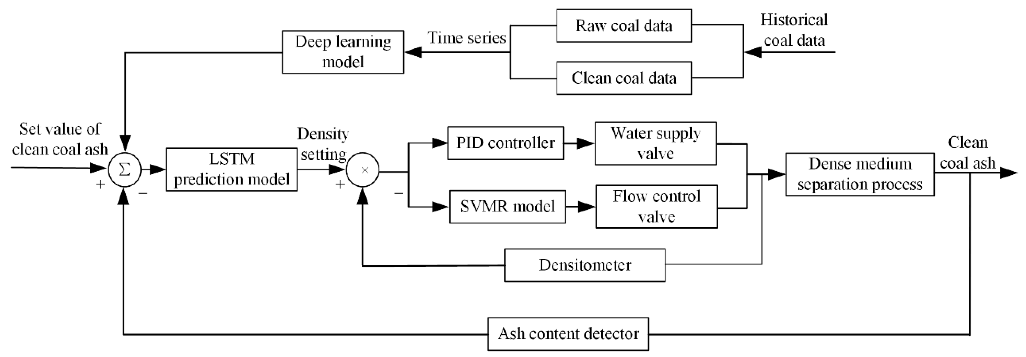
Figure 1 illustrates the control system, which is a two-layer nested closed-loop control system, of dense medium separation. The outer ring is the feedback control of clean coal ash, which is used to control the quality of clean coal products; the inner ring is the feedback control of suspension density. In a traditional dense medium separation process, feedback is adjusted through manual operations, thus, a substantial time lag exists in all the operational aspects such as production and detection [15,16,17]. Therefore, the dense medium separation control system is divided into three parts: clean coal ash feedback, suspension density prediction, and suspension density control. In clean coal ash feedback, a clean coal ash analyzer is used to detect the ash content in real time and to feed it back to the control system. The suspension density prediction part employs the LSTM method to predict suspension density in real time. Simultaneously, according to the online ash content data, the predicted density value is finetuned to enhance system robustness. The suspension density control part is composed of water supply and flow control valves controlled by ta Proportion Integration Differentiation (PID) controller and Support Vector Machine Regression (SVMR) prediction model, respectively. By using the feedback of a densitometer, the openings of water supply and flow control valves are finetuned to increase system stability. These three parts interact with and influence each other.
Assume that at time T, the measured ash content of raw coal and clean coal, suspension density are Adi(T), Adj(T), d(T), respectively. First, the raw coal is mixed with the suspension after it passes through a conveyor belt, and then it is sent to a separation sorting system. After separation and dewatering, the ash content of the product is measured using an ash content detector on a clean coal conveyor. Therefore, a change of in raw coal ash at time T affects product ash at time (T + t1), and a change in suspension density at time T influences product ash at time (T + t2), where t1 and t2 are the lag time of raw coal ash and suspension density affecting clean coal ash, respectively.
To eliminate the influence of the lag time on the density control system, an LSTM method that can solve the problems related to the short-term time series was employed to establish a relation between the ash content and suspension density. The relationship between density and ash is expressed as follows:
where ρ is the suspension density, and Adi(T) and Adj(T) are the raw and clean coal ash corresponding to time T, respectively.
2.2. LSTM Prediction Method
2.2.1. Dataset Preparation
The data used were obtained from the historical production data of the dense medium separation system of a coal preparation plant in Inner Mongolia, China. Due to many factors (such as sensor failure, network interruption, server failure) that influenced data storage and collection processes, the collected data was inevitably abnormal and presented missing cases. For these data, as time series requires equal time gaps between data samples, it could not be eliminated directly as in other networks, therefore, the data must be replaced and filled reasonably.
The moving average method was used to resolve abnormal data problems, and the calculation formula used is as follows:
where the abnormal data at time T are replaced by XT, and b is the initial calculation sequence point.
The cubic exponential smoothing method was employed to fill in the missing data. Exponential smoothing can be divided into single, second, and cubic exponential smoothing methods based on smoothing numbers. The single exponential smoothing method is relatively simple; however, it cannot reflect the time series trend. The second exponential smoothing method can be employed to adjust the predicted value with the parabolic growth of the time series, but when the quadratic curve trend appears during the changing of the time series, the cubic exponential smoothing method must be used. The cubic exponential smoothing method, which can ensure the smoothness of missing values and inherit the trend of the original time series, is almost suitable for analyzing all application problems of the time series, to prevent the training results from being influenced because of the missing data [18,19]. The calculation formula is as follows:
where Xt+L is the replacement value of a missing point, L is the length of a smoothing step, and at, bt and ct are the parameters of cubic exponential smoothing respectively, which can be obtained from the following formula:
where α is the weight parameter and its value is in between 0 and 1, and the first, second, and third derivatives of St are the first, second, and third exponential smoothing values at time t, respectively. The calculation formula is as follows:
After the preprocessing of data, the time series data for model training were obtained.
2.2.2. LSTM Method
With the rapid development of neural networks, LSTM network are widely used in the deep learning field. Compared with basic neural networks, the LSTM network establishes weight connections not only between different layers but also in the same layer. The LSTM network is a type of Recurrent Neural Network (RNN) that relies on the time series. RNN recurses in the direction of sequence evolution and links all nodes in a chain. The nature of this chain-link reveals the close relationship between sequences. Because LSTM is used to solve the gradient disappearance problem when RNN is employed to process the long-sequence data, LSTM is suitable for processing events with relatively long intervals and delays, such as speech recognition, machine translation, and time series prediction, in the time series [20,21,22].
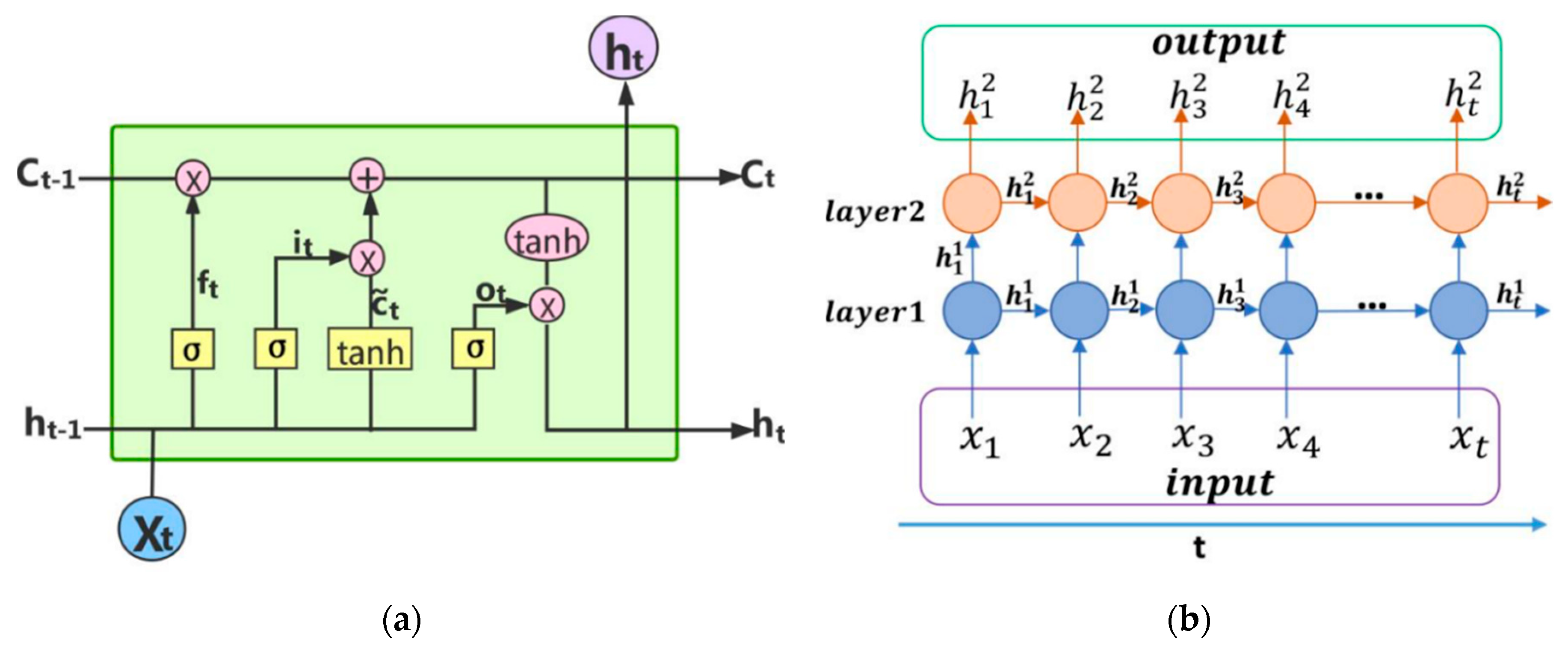
Figure 2a presents the internal work unit of the LSTM network. The unit receives input information xt of the current moment and hidden state ht−1 and unit state Ct−1 of the previous moment. The information is transmitted and suppressed by three gates, namely forget, gate, and output gates. The forget gate determines the amount of ‘forgotten’ information about the hidden state ht−1 of the previous moment through a sigmoid activation function. The input gate has two functions: (1) select values to reserve by using the sigmoid function(σ), (2) generate candidate vector values by using the tanh activation function(tanh). The product of the reserved value and candidate vector is considered a part of the state quantity. The sum of this state quantity and the product of ft generated in the forget gate and the state quantity of the previous time is used as the current unit state Ct. Finally, the output gate generates candidate vectors through tanh, selects the retained information through the sigmoid function, and simultaneously transmits result ht as the current hidden state to the next unit and the unit in the previous layer. The complete calculation process of LSTM is as follows:
Forget gate:
Input gate:
Cell:
Output gate:
where Wf, Wi, Wc, and Wo represent the weight vectors of the forget gate, input gate, cell state, and output gate respectively; bf, bi, bc, and bo represent the bias vectors of the forget gate, input gate, cell state, and output gate respectively; and σ is the sigmoid activation function.
Figure 2b presents the working principle of the LSTM network, which is a structure with t time steps and two network layers. x1, x2, x3, x4, …, xt are the preprocessed time series data. After receiving input data x1, the first work unit of the first layer calculates the current response with the initialized unit and hidden states and transmits response to the second and first units in the previous layer. The second work unit of the first layer receives input data x2 and the state quantity of previous unit at the next moment, and then transmits the result to the third and the second units in the second layer, and so on. The unit of the second layer receives the output of the first layer as an input, it transmits the calculation result in the same manner as the first layer does, and it provides the hidden state of each unit as the output at each time step.
2.2.3. Modelling Methods
The experimental program was written in Python 3.5 and used deep learning library Keras 2.2.4 and deep learning framework Tensorflow 2.0.
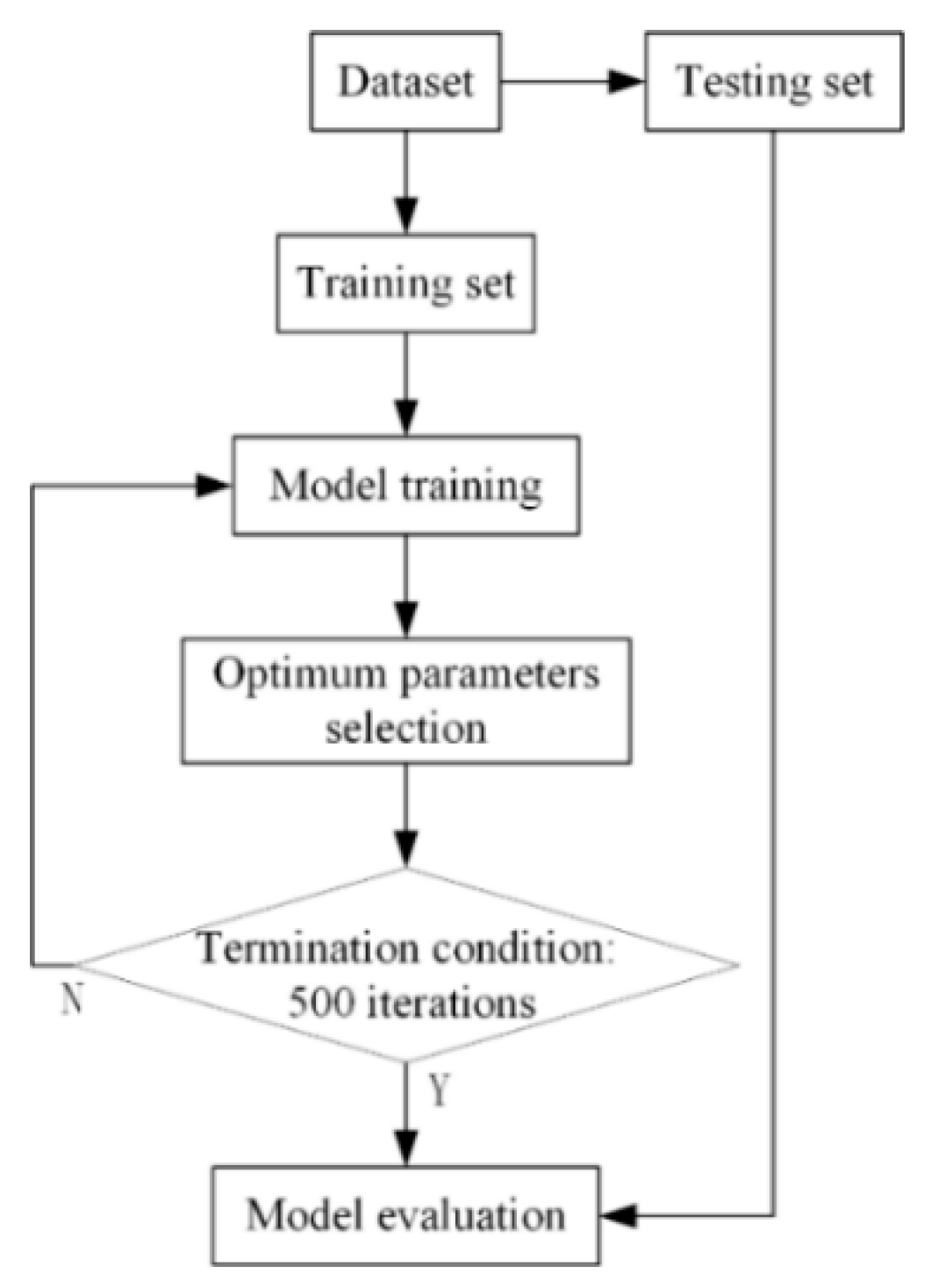
Figure 3 shows the process of LSTM prediction. First, the preprocessed data were divided into training set and testing sets, and the training set was used to train the model. Subsequently, model parameters were adjusted to select the optimum parameters. After the selection the optimum parameters, the model was trained for 500 iterations. Finally, the model performed evaluation by using the testing set data.
2.2.4. Comparison Algorithm
To verify that the model provides satisfactory prediction, the LSTM prediction method was compared with the widely used BP prediction method. The BP neural network is a multilayer feedforward neural network trained according to the error back propagation algorithm. Its basic algorithm includes two processes: forward propagation of signals and back propagation of errors. The basic idea of BP neural network is the gradient descent method, which uses gradient search to minimize the mean square error between the actual and expected output values [23,24].
2.2.5. Prediction Performance Indicators
To validate and compare model performance, different validation criteria, such as RMSE and MAPE, were employed. They were used to evaluate the errors of the trained models, MAPE was used to calculate the average percentage difference between the measured and predicted values without consideration of their weight and direction, and RMSE is defined as the square median root the squared difference between measured and predicted values [25,26,27]. The calculations of RMSE and MAPE are based on the following Equations:
where m is the total number of the data samples, yt indicates the actual value of the sample, and yp indicates the predicted value of the sample.
3. Results and Discussion
3.1. Data Preprocessing
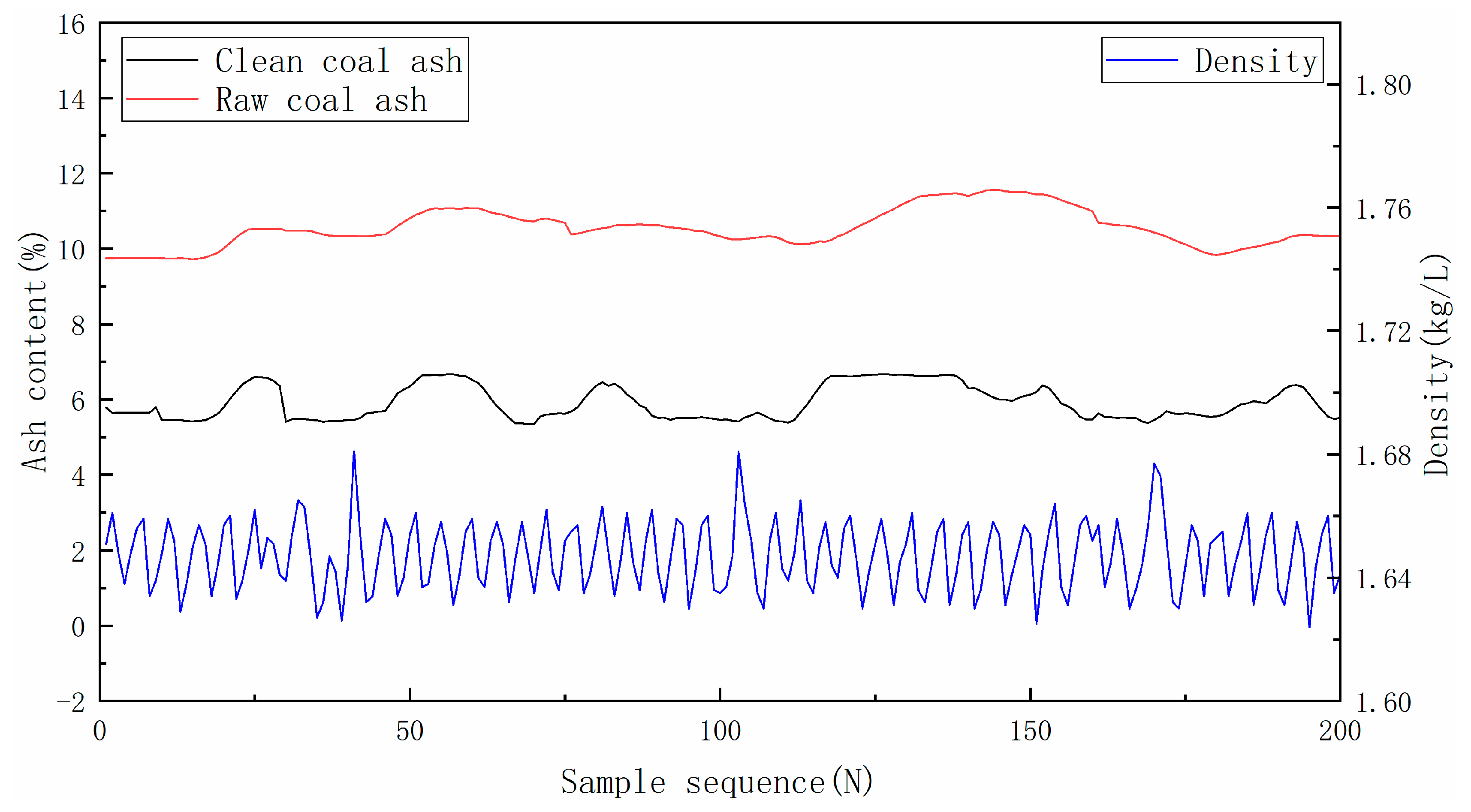
This study used 200 data samples, of which the first 160 were the training set (80%), and the last 40 were the testing set (20%). Figure 4 presents raw coal ash, clean coal ash, and suspension density data obtained after replacing the abnormal data with the moving average method and filling the missing data with the cubic exponential smoothing method. Table 1 the maximum, minimum and mean values of the sample data.
3.2. Optimum Parameter Selection
Parameters that must be adjusted in the LSTM network include the number of input layer nodes, output layer nodes, hidden layer nodes, hidden layers, time steps, and learning rate. The input layer is a two-dimensional time series composed of raw and clean coal ash, and the output layer is the one-dimensional data for predicting suspension density. Because the values of the suspension density were small, the learning rate parameter was set to 0.0001. Therefore, the parameters adjusted were the number of hidden layers, hidden layer nodes, and time steps.
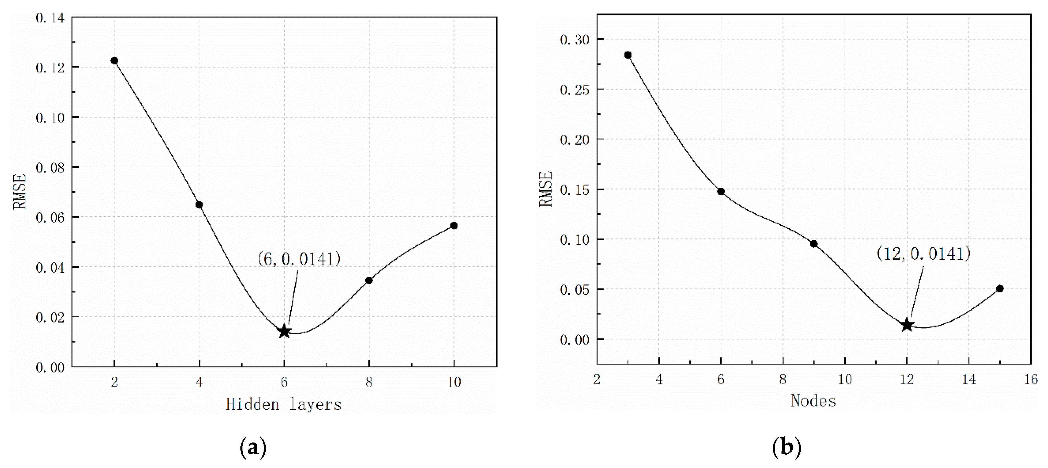
To select the optimal number of hidden layers and nodes, 25 LSTM network combinations with 3, 6, 9, 12, and 15 nodes and 2, 4, 6, 8, and 10 hidden layers were designed. The number of time steps was set to the default value of none. Table 2 presents the RMSE of different combinations. Figure 5 shows how RMSE changes with different hidden layers and nodes. When the number of hidden layers and nodes was 6 and 12, respectively, RMSE reached a minimum value of 0.0141. A large number of hidden layers and nodes increases the model complexity and training time, and the accuracy does not improve. Therefore, the LSTM network structure with 6 hidden layers and 12 nodes was selected.
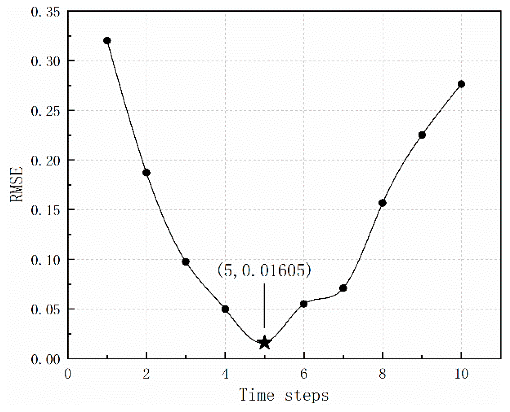
Another parameter that must be determined is the number of time steps (i.e., delay time). Figure 6 shows the effect of time steps on the model accuracy for 6 hidden layers and 12 nodes. The prediction accuracy was the highest when the number of time steps was 5, and the corresponding RMSE was 0.01605 (Figure 6).
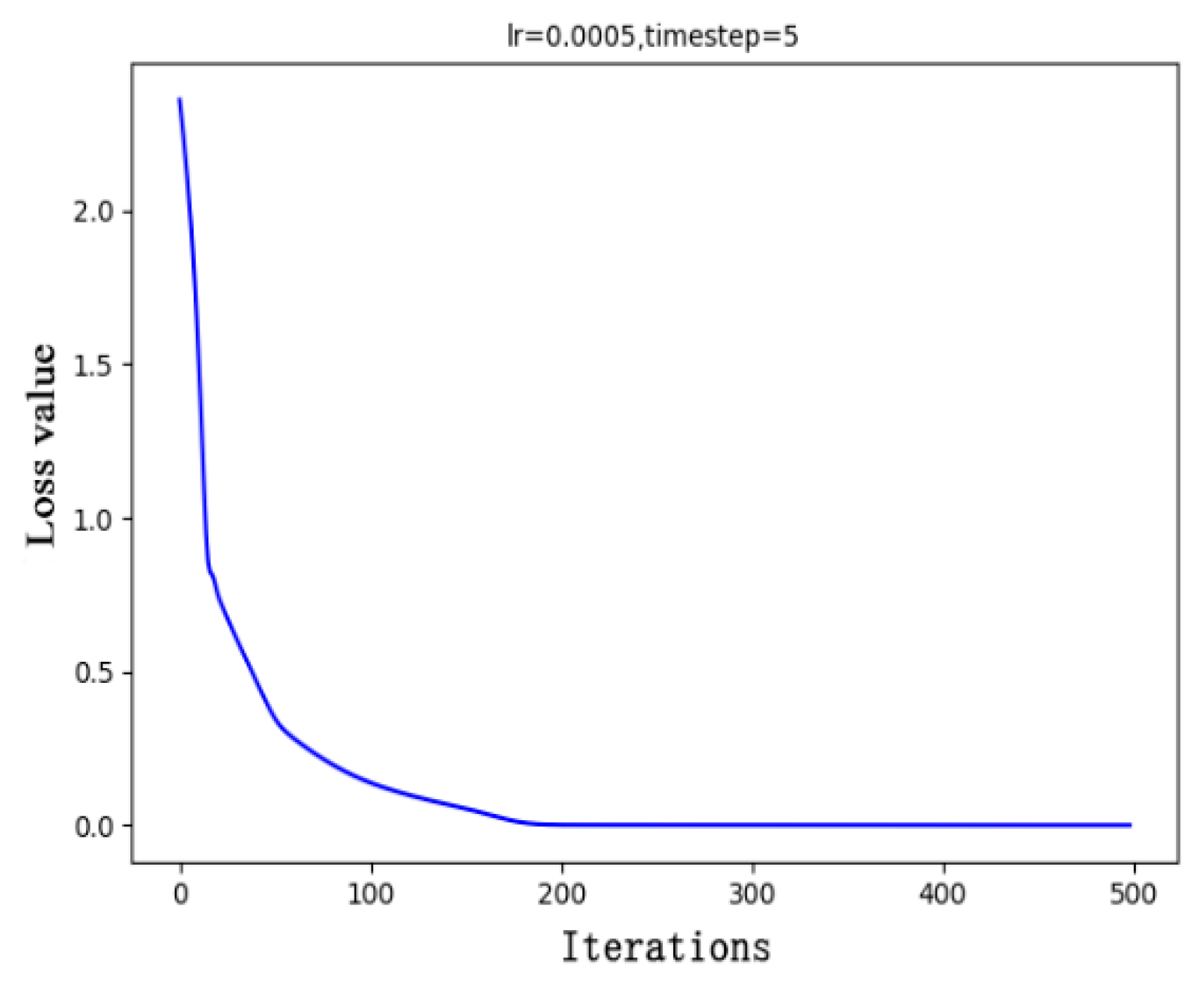
The model weight was initialized using the Xavier method. The dropout layer was added to prevent overfitting. The Adam adaptive learning rate algorithm was used to optimize the gradient descent process, and a session training model was constructed. The model was iterated 500 times, and Figure 7 presents the change in the loss values. The model converged after approximately 200 iterations.
3.3. Modelling Performance
The trained LSTM prediction model was evaluated according to the testing set and compared with the BP method without the time series. After the test, the optimal structure of the BP prediction model comprised 5 hidden layers, each of which contained 10 neurons. The same training and testing sets were used in the BP method as in LSTM.
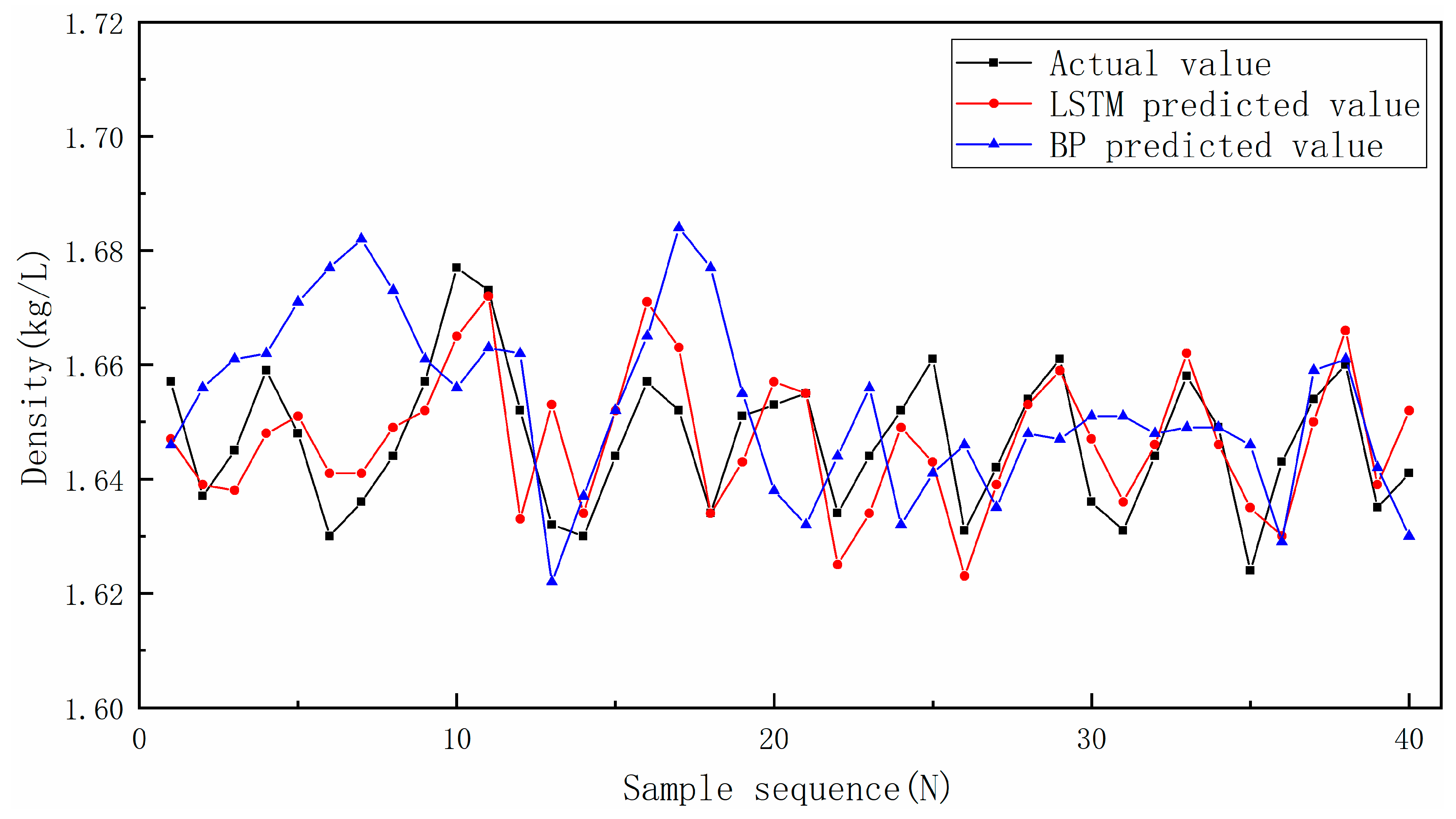
Figure 8 shows the performance of LSTM and BP methods on the testing set. Compared with the BP method, the predicted value and tendency of the LSTM method were highly consistent with the actual value and trend of the actual value, respectively. The performance of the BP method was unsatisfactory.
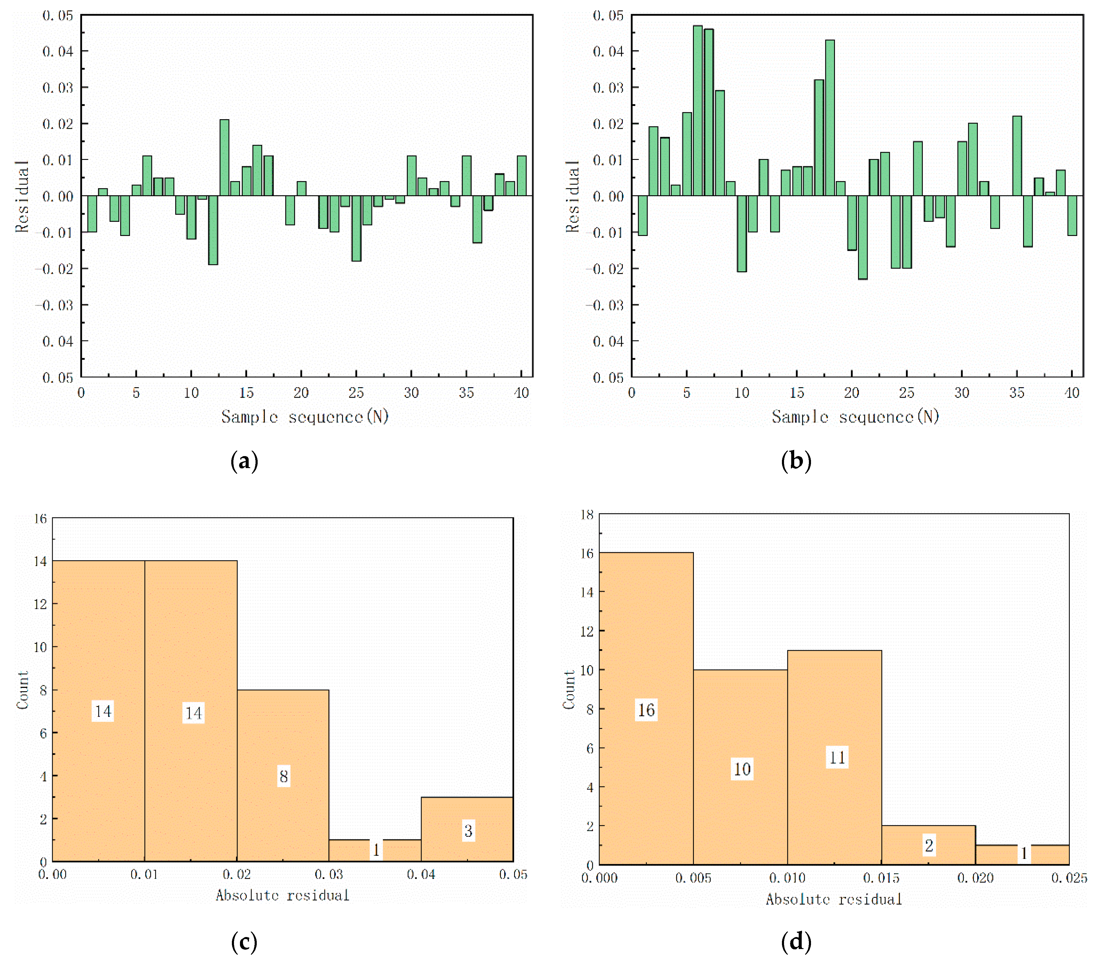
Figure 9 shows the residual values (predicted values minus actual values) of the two models. The maximum and minimum residual values of the LSTM method were 0.021 and −0.019, respectively (Figure 9a). However, only a few samples received relatively large prediction errors, and most residual values were between −0.015 and 0.015. Figure 9c shows the distribution of absolute residual values, which can further elucidate this phenomenon. The absolute residual values of the most samples (82.2%) in the testing set were approximately or below 0.015, which indicated that the model provides considerably satisfactory prediction for most samples (Figure 9c). However, the maximum and minimum residual values of the BP method were 0.023 and −0.047, respectively (Figure 9b). Furthermore, 30% absolute residual values remained higher than 0.02 (Figure 9d). Although most residual values can be controlled within ±0.02, its tendency did not fit well to the actual trend.
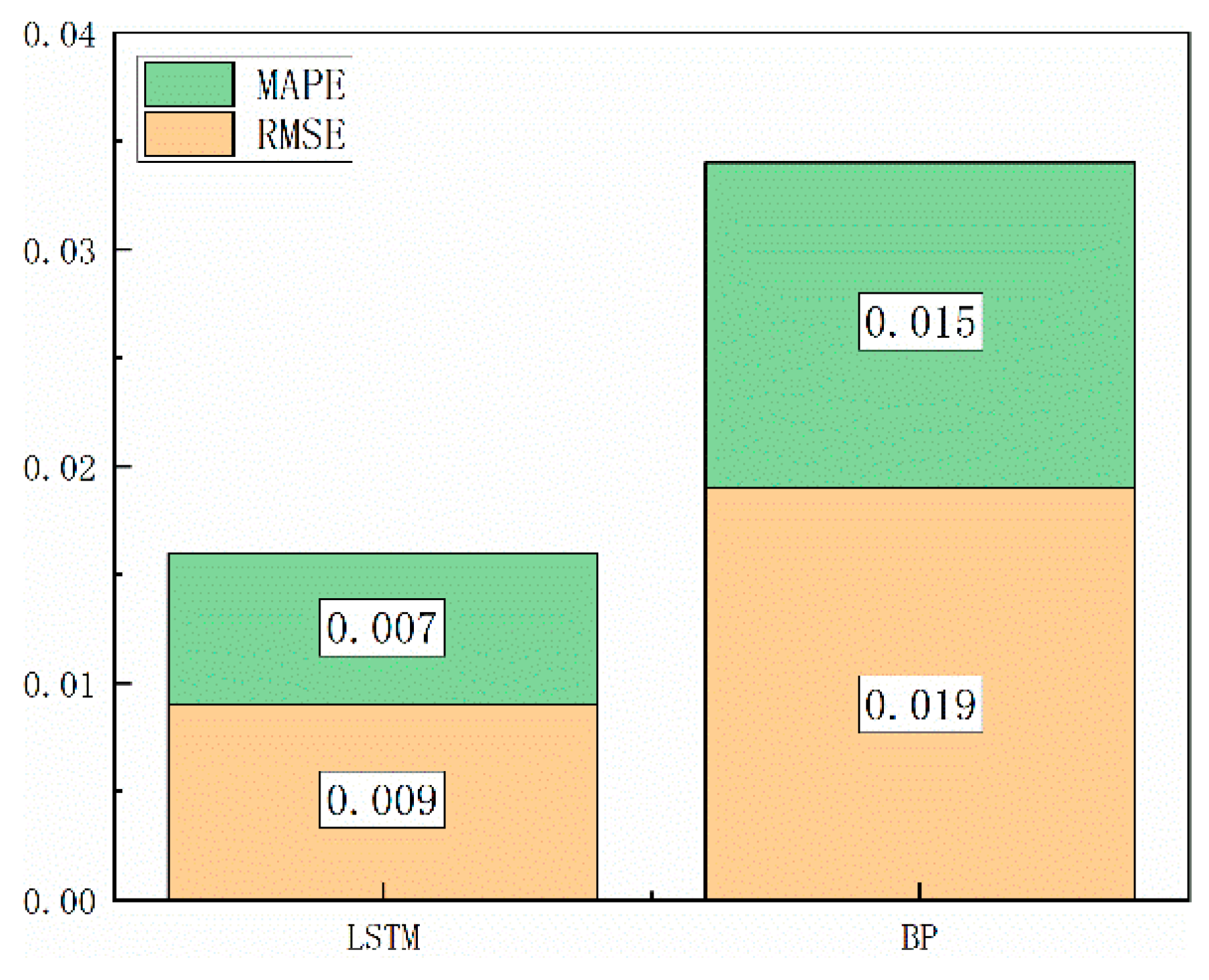
Table 3 presents the validation criteria results of the two prediction models. The RMSE and MAPE of the LSTM method were 0.009 and 0.007, respectively, and those of the BP method were 0.019 and 0.015, respectively. Figure 10 presents the error figure of the two methods to visually show the difference. Compared with the BP method, the LSTM prediction model achieved better prediction results.
The results showed that the prediction model of suspension density established using the LSTM network can reduce the time-lag influence. Compared with the BP method, the error of the LSTM method is smaller, and its tendency is well fitted to the actual trend.
Therefore, the prediction model of suspension density based on LSTM can accurately predict the suspension density of the dense medium separation system. It can solve the time-lag problem and adjust suspension density more promptly. In turn, clean coal ash was stabilized, and the efficiency of dense medium separation was improved.
4. Conclusions
To solve the problem of unstable product quality caused by the fluctuations of raw coal ash and the lag of suspension density adjustment during the dense medium separation system, a prediction model of suspension density based on the LSTM method was established. The historical data in the dense medium separation system of the coal preparation plant in Inner Mongolia, China, were used for simulations. The prediction accuracy of the LSTM method reaches the highest when the number of hidden layers, nodes, and time steps of the model is 6, 12, and 5, respectively. At this time, the MAPE and RMSE of the model are 0.007 and 0.009, respectively, which are better than those of the BP method. The LSTM method not only provides high prediction accuracy but also is well fitted to the actual trend. Therefore, the prediction model of suspension density based on LSTM can be used to accurately predict the suspension density of the dense medium separation system.
Author Contributions
Conceptualization, J.D.; data curation, C.Z.; formal analysis, Z.H.; funding acquisition, J.D.; investigation, G.W.; methodology, C.Z. and J.D.; project administration, J.D.; software, Z.H.; validation, Z.H. and G.W.; Writing—original draft, C.Z.; writing—review & editing, C.Z. All authors have read and agreed to the published version of the manuscript.
Funding
This research was funded by the National Natural Science Foundation of China, grant number 51604273, and the Fundamental Research Funds for the Central Universities, grant number 2014QNB14.
Conflicts of Interest
The authors declare no conflict of interest.
References
- Napier-Munn, T.J. Modelling and simulating dense medium separation processes—A progress report. Miner. Eng. 1991, 4, 329–346. [Google Scholar] [CrossRef]
- Sahu, A.K.; Biswal, S.K.; Parida, A. Development of air dense medium fluidized bed technology for dry beneficiation of coal—A review. Coal Prep. 2009, 29, 216–241. [Google Scholar] [CrossRef]
- Honaker, R.Q.; Singh, N.; Govindarajan, B. Application of dense-medium in an enhanced gravity separator for fine coal cleaning. Miner. Eng. 2000, 13, 415–427. [Google Scholar] [CrossRef]
- Dai, W.; Zhang, L.; Fu, J.; Chai, T.; Ma, X. Model-data-based switching adaptive control for dense medium separation in coal beneficiation. Control Eng. Pract. 2020, 98, 104241. [Google Scholar] [CrossRef]
- Wang, Z.; Kuang, Y.; Deng, J.; Wang, G.; Ji, L. Research on the intelligent control of the dense medium separation process in coal preparation plant. Int. J. Miner. Process. 2015, 142, 46–50. [Google Scholar] [CrossRef]
- Meyer, E.J.; Craig, I.K. Coal dense medium separation dynamic and steady-state modelling for process control. Miner. Eng. 2014, 65, 98–108. [Google Scholar] [CrossRef] [Green Version]
- Sun, X.; Cao, Z.; Yue, Y.; Kuang, Y.; Zhou, C. Online prediction of dense medium suspension density based on phase space reconstruction. Part. Sci. Technol. 2018, 36, 989–998. [Google Scholar] [CrossRef]
- Fan, P.; Fan, M.; Liu, A. Using an axial electromagnetic field to improve the separation density of a dense medium cyclone. Miner. Eng. 2015, 72, 87–93. [Google Scholar] [CrossRef]
- Chu, K.; Wang, B.; Yu, A.; Vince, A. Modelling the Multiphase Flow in Dense Medium Cyclones. J. Comput. Multiph. Flows 2010, 2, 249–272. [Google Scholar] [CrossRef] [Green Version]
- Chu, K.; Wang, B.; Yu, A.; Vince, A. CFD-DEM modelling of multiphase flow in dense medium cyclones. Powder Technol. 2009, 193, 235–247. [Google Scholar] [CrossRef]
- Magwai, M.K.; Bosman, J. The effect of cyclone geometry and operating conditions on spigot capacity of dense medium cyclones. Int. J. Miner. Process. 2008, 86, 94–103. [Google Scholar] [CrossRef]
- Hu, S.; Firth, B.; Vince, A.; Lees, G. Prediction of dense medium cyclone performance from large size density tracer test. Miner. Eng. 2001, 14, 741–751. [Google Scholar] [CrossRef]
- Fanayi, A.R.; Nikbakht, A.M. Study of gas-solid flow in a cyclone separator. Int. J. Food Eng. 2015, 11, 71–77. [Google Scholar]
- Wang, G.; Kuang, Y.; Wang, Z.; Wang, Y.; Ji, L. A real-time prediction model for production index in process of dense-medium separation. Int. J. Coal Prep. Util. 2012, 32, 298–309. [Google Scholar]
- Meyer, E.J.; Craig, I.K. Dynamic model for a dense medium drum separator in coal beneficiation. Miner. Eng. 2015, 77, 78–85. [Google Scholar] [CrossRef] [Green Version]
- Chen, J.; Chu, K.; Zou, R.P.; Yu, A.; Vince, A. Prediction of the performance of dense medium cyclones in coal preparation. Miner. Eng. 2012, 31, 59–70. [Google Scholar] [CrossRef]
- Kumar, C.R.; Mohanan, S.; Tripathy, S.K.; Ramamurthy, Y.; Venugopalan, T.; Suresh, N. Prediction of process input interactions of floatex density separator performance for separating medium density particles. Int. J. Miner. Process. 2011, 200, 136–141. [Google Scholar] [CrossRef]
- Wang, J.; Yang, W.; Cheng, H.; Huang, L.; Gao, Y. The Optimal Configuration Scheme of the Virtual Power Plant Considering Benefits and Risks of Investors. Energies 2017, 10, 968. [Google Scholar] [CrossRef] [Green Version]
- Zhang, Y.; Guo, E. The study of forecasting of cash flow in ATM based on cubic exponential smoothing method. Biotechnol. Indian J. 2014, 10, 2501–2506. [Google Scholar]
- Muzaffar, S.; Afshari, A. Short-Term Load Forecasts Using LSTM Networks. Energy Procedia 2019, 158, 2922–2927. [Google Scholar] [CrossRef]
- Li, X.; Peng, L.; Yao, X.; Cui, S.; Hu, Y.; You, C.; Chi, T. Long short-term memory neural network for air pollutant concentration predictions: Method development and evaluation. Environ. Pollut. 2017, 231, 997–1004. [Google Scholar] [CrossRef] [PubMed]
- Gers, F.A.; Schmidhuber, J.; Cummins, F. Learning to Forget: Continual Prediction with LSTM. Neural Comput. 2000, 12, 2451–2471. [Google Scholar] [CrossRef] [PubMed]
- Wang, Z.; Wang, F.; Su, S. Solar Irradiance Short-Term Prediction Model Based on BP Neural Network. Energy Procedia 2011, 12, 488–494. [Google Scholar] [CrossRef] [Green Version]
- Li, J.; Zhao, D.; Ge, B.; Yang, K.; Chen, Y. A link prediction method for heterogeneous networks based on BP neural network. Phys. A Stat. Mech. Appl. 2017, 496, 1–17. [Google Scholar] [CrossRef]
- Qi, C.; Ly, H.; Chen, Q.; Le, T.; Le, V.M.; Pham, B.T. Flocculation-dewatering prediction of fine mineral tailings using a hybrid machine learning approach. Chemosphere 2019, 244, 125450. [Google Scholar] [CrossRef]
- Qi, C.; Fourie, A.; Chen, Q.; Tang, X.; Zhang, Q.; Gao, R. Data-driven modelling of the flocculation process on mineral processing tailings treatment. J. Clean. Prod. 2018, 196, 505–516. [Google Scholar] [CrossRef]
- Massinaei, M.; Jahedsaravani, A.; Taheri, E.; Khalilpour, J. Machine vision based monitoring and analysis of a coal column flotation circuit. Powder Technol. 2019, 343, 330–341. [Google Scholar] [CrossRef]
Figure 1.
Dense medium separation control system.

Figure 2.
Internal and external structure of LSTM (a) cell and (b) network layers.

Figure 3.
Process of LSTM prediction.

Figure 4.
Preprocessed data.

Figure 5.
Root Mean Squared Error (RMSE) with different (a) hidden layers, and (b) nodes.

Figure 6.
Root Mean Squared Error (RMSE) with different time steps.

Figure 7.
Model convergence process.

Figure 8.
Performance of two models on the testing set.

Figure 9.
Residual of (a) LSTM, and (b) BP methods on the testing set; distribution diagram of the absolute residual values of (c) LSTM, and (d) BP methods.
Figure 9.
Residual of (a) LSTM, and (b) BP methods on the testing set; distribution diagram of the absolute residual values of (c) LSTM, and (d) BP methods.

Figure 10.
Error figure of the two methods.


Table 1.
Data set statistics table.
| Statistics | Raw Coal Ash (%) | Clean Coal Ash (%) | Suspension Density (g/cm3) |
|---|---|---|---|
| Maximum Value | 11.56 | 6.67 | 1.681 |
| Minimum Value | 9.65 | 5.35 | 1.624 |
| Mean Value | 10.46 | 5.87 | 1.650 |
Table 2.
RMSE of different hidden layers and nodes.
| Nodes | 3 | 6 | 9 | 12 | 15 | |
|---|---|---|---|---|---|---|
| Hidden Layers | ||||||
| 2 | 0.2298 | 0.1237 | 0.0975 | 0.1225 | 0.1572 | |
| 4 | 0.3143 | 0.1817 | 0.1149 | 0.0648 | 0.0872 | |
| 6 | 0.2841 | 0.1476 | 0.0950 | 0.0141 | 0.0503 | |
| 8 | 0.2020 | 0.1141 | 0.0707 | 0.0346 | 0.0200 | |
| 10 | 0.1865 | 0.0977 | 0.0479 | 0.0564 | 0.0721 | |
Table 3.
Validation criteria results.
| Validation Criteria | LSTM | BP |
|---|---|---|
| RMSE | 0.009 | 0.019 |
| MAPE | 0.007 | 0.015 |
© 2020 by the authors. Licensee MDPI, Basel, Switzerland. This article is an open access article distributed under the terms and conditions of the Creative Commons Attribution (CC BY) license (http://creativecommons.org/licenses/by/4.0/).
Share and Cite
MDPI and ACS Style
Zheng, C.; Deng, J.; Hong, Z.; Wang, G. Prediction Model of Suspension Density in the Dense Medium Separation System Based on LSTM. Processes 2020, 8, 976. https://0-doi-org.brum.beds.ac.uk/10.3390/pr8080976
AMA Style
Zheng C, Deng J, Hong Z, Wang G. Prediction Model of Suspension Density in the Dense Medium Separation System Based on LSTM. Processes. 2020; 8(8):976. https://0-doi-org.brum.beds.ac.uk/10.3390/pr8080976
Chicago/Turabian StyleZheng, Cheng, Jianjun Deng, Zhixin Hong, and Guanghui Wang. 2020. "Prediction Model of Suspension Density in the Dense Medium Separation System Based on LSTM" Processes 8, no. 8: 976. https://0-doi-org.brum.beds.ac.uk/10.3390/pr8080976
Note that from the first issue of 2016, this journal uses article numbers instead of page numbers. See further details here.