Grand Tour Algorithm: Novel Swarm-Based Optimization for High-Dimensional Problems


1
Department of Hydraulic Engineering and Water Resources-ERH, Universidade Federal de Minas Gerais, Belo Horizonte 31270-901, Brazil
2
Fluing-Institute for Multidisciplinary Mathematics, Universitat Politècnica de València, Camino de Vera s/n, 46022 Valencia, Spain
3
Department of Water Resources-DRH, Universidade Estadual de Campinas, Campinas 13083-889, Brazil
*
Author to whom correspondence should be addressed.
Processes 2020, 8(8), 980; https://0-doi-org.brum.beds.ac.uk/10.3390/pr8080980
Submission received: 29 June 2020
/
Revised: 6 August 2020
/
Accepted: 11 August 2020
/
Published: 13 August 2020
(This article belongs to the Special Issue Control and Optimization of Multi-Agent Systems and Complex Networks for Systems Engineering)
Abstract
:Agent-based algorithms, based on the collective behavior of natural social groups, exploit innate swarm intelligence to produce metaheuristic methodologies to explore optimal solutions for diverse processes in systems engineering and other sciences. Especially for complex problems, the processing time, and the chance to achieve a local optimal solution, are drawbacks of these algorithms, and to date, none has proved its superiority. In this paper, an improved swarm optimization technique, named Grand Tour Algorithm (GTA), based on the behavior of a peloton of cyclists, which embodies relevant physical concepts, is introduced and applied to fourteen benchmarking optimization problems to evaluate its performance in comparison to four other popular classical optimization metaheuristic algorithms. These problems are tackled initially, for comparison purposes, with 1000 variables. Then, they are confronted with up to 20,000 variables, a really large number, inspired in the human genome. The obtained results show that GTA clearly outperforms the other algorithms. To strengthen GTA’s value, various sensitivity analyses are performed to verify the minimal influence of the initial parameters on efficiency. It is demonstrated that the GTA fulfils the fundamental requirements of an optimization algorithm such as ease of implementation, speed of convergence, and reliability. Since optimization permeates modeling and simulation, we finally propose that GTA will be appealing for the agent-based community, and of great help for a wide variety of agent-based applications.
1. Introduction
Many optimization problems in engineering are of a very complex nature and must be solved in accordance with various, sometimes complicated constraints. As a consequence, finding an optimal solution is often hard. In addition, frequently, a large number of mixed variables, and differential and nonlinear equations, are used to describe the problem. As a result, in many cases, classical optimization procedures based on differential methods cannot be used. Metaheuristic techniques arise to bridge this gap, as they can explore the search space for optimal and feasible solutions in a less restrictive (derivative-free) framework. Since in continuous problems, the set of feasible solutions is infinite, metaheuristic algorithms use empirical iterative search methods, based on various heuristics, to guide the search in a way that the solution is expected to always improve.
As described in [1], metaheuristic algorithms are often inspired by nature, and can be classified into the following groups: (i) evolutionary, inspired from biology, where an initial population evolves over generations; (ii) swarm intelligence, inspired from the social behavior of animals; (iii) physics-based, inspired by natural phenomena; and (iv) human related, inspired from human beings and their physical and mental activities.
In swarm intelligence techniques, the social features of a group are used to define the behavior of its individuals, leading to (local) optimal solutions [2]. In general, the position of an individual represents a potential solution, and has a defined score based on the objective function of interest. First, initial positions for individuals are defined randomly, and this defines their initial score. Then, an individual evolves according to: (i) its own preferences, based on its past experience, i.e., on its best performance ever achieved, and (ii) according to the group experience, i.e., the best solution ever found by any individual in the group. Each algorithm has its own rules to express this social behavior. Additional random coefficients are used to guarantee better exploration of the search space, especially in the initial period, and those coefficients are also modified across iterations [3] to achieve better exploitation, mainly at the end of the search. In addition, the historical evolutionary information deployed by swarm algorithms can be efficiently used in dynamic optimization to detect the emergent behaviors of any involved agent or element. Examples are algorithms based on ants [4] and bees [5] looking for food, the breeding behavior of cuckoos [6], the behavior of flocking birds [7], among many others. Extensive lists of algorithms belonging to the four abovementioned categories of metaheuristics algorithms can be found in [1]. Specifically, Table 2 in [1] compiles 76 swarm intelligence algorithms, together with some specific details.
Physics-based algorithms mimic the behavior of natural phenomena and use the rules governing these phenomena to produce optimal solutions. Perhaps the most popular of these algorithms is simulated annealing [8], based on crystal development in metallurgy. Table 3 in [1] provides a list of 36 physics-based algorithms, together with basic information about them.
One of the major issues of metaheuristic algorithms is the fact that there is no guarantee that the global optimal solution is obtained. Despite the randomness deployed to build the initial solutions and during each iteration, the search can be easily biased, and the final result may be just a point that is close to a local optimum [9]. In addition, to account for possible constraints of the problem, in a single-objective setting, penalty functions have to be used, adding a value to the objective function to hinder unfeasible solutions [10]. If the added value is too high, optimal solutions on the boundaries can be disregarded because of the steep path this represents for the individuals and the strong deformation of the objective function landscape close to the boundary. On the other hand, if the penalty is too soft, unfeasible solutions can be considered as optimal [11]. The randomness of the process and the penalties added can lead to inconsistent results, so that multiple runs of the algorithm are necessary to verify the quality of the solution.
Another crucial issue of these methods is the computational effort required. Multiple solutions (individuals) must be evaluated in each iteration. This number varies according to the number of variables comprising the problem, and can be very large. In general, the number of individuals has to be at least the same as the number of variables [12]. Thus, in complex problems, the number of objective function evaluations can be huge. In addition, many engineering problems use external models to calculate the parameters of the objective function and the constraints, as is the case with hydraulic [13], thermal [14], and chemical models [15], thus increasing even more the computational effort required.
Swarm intelligence in general, and the metaheuristic we develop in this paper in particular, may have a number of benefits for many agent-based models (ABM) and applications. Among the benefits derived from applying optimization in ABM, we briefly mention the following: (a) simulation reuse facility, since there is a generalized demand for improved methods for studying many complex environments as integrated wholes [16,17,18,19]; (b) dynamic optimization due to problem uncertainty, especially in cases of slow changes, i.e., those most commonly occurring in real-world applications [20,21,22]; (c) the ability to identify emergent behaviors and conditions for them [23,24,25]; this provides insights into the landscape of system performance to help identify elements that exhibit emergent behavior where the system performance rapidly improves because it moves from disorganized to organized behavior; (d) simulation cloning to analyze alternative scenarios concurrently within a simulation execution session [26,27]; this would help optimize the execution time for multiple evaluations without repeated computation [28].
A final crucial idea is that there is no such a thing as the best metaheuristic algorithm; rather, each has advantages and disadvantages. In fact, [29,30] propose a multi-agent approach to take the best of multiple algorithms. Each of them considers separated agents searching for their own goals, and also competing and cooperating with others to reach a common goal. In general, an optimization algorithm is evaluated regarding three major aspects [31]: (i) ease of implementation due to the number of parameters to be adjusted (sometimes costly fine-tuned); (ii) computational complexity, which reflects in the convergence speed; and (iii) reliability of the results, with consistent optimal values obtained through a series of tests.
As an attempt to help to solve these problems, a novel, hybrid, swarm-physics-based algorithm that uses the metaphor of cyclists’ behavior in a peloton, which we have named the Grand Tour Algorithm (GTA), is proposed in this paper. The main features of the algorithm are: (i) the drag, defined according to the distance to the leading cyclist (embodying the best solution), and (ii) the speed, defined using the difference between two consecutive objective function evaluations. These two elements are used to calculate the coefficients that determine the route of each cyclist. As a result, the peloton will try to follow the cyclist who is closest to the finish line, i.e., the optimal solution, and also, the cyclist who is going fastest at a given point. In Section 2, we describe the methodological aspects first. Then, we set the test conditions. These include the fourteen benchmarking functions used, and the complete setting of parameters for the four classical metaheuristic algorithms used for comparison: Particle Swarm Optimization [7], Simulated Annealing [8], Genetic Algorithm [32] and Harmony Search [33]. In Section 3, comparisons are performed under a scenario of 1000 variables, which are used to evaluate the performance of the algorithms under a generally accepted metric. In addition, the algorithms are also applied to the same fourteen functions when their dimension is up to 20,000 variables. Finally, various sensitivity analyses verify the relevance the algorithm parameters have in the optimization convergence and stability of GTA. To finish, conclusions are presented that provide evidence that GTA (i) is superior to other classical algorithms in terms of its speed and consistency when functions with a huge (human genome-like) search space are considered, and (ii) exhibits excellent results regarding ease of implementation, speed of convergence and reliability.
2. Materials and Methods
In this section, we present a few general ideas about iterative methods. Then, we concisely describe the classical PSO, which has the basic foundations of any swarm-based algorithm. Finally, we fully present GTA.
2.1. Iterative Optimization Processes: A General View
Typically, an iterative optimization algorithm can be mathematically described, as in Equation (1):
where is (the position of) a solution at time step , is the step size, and is the direction of the movement.
Since there is no general a priori clue about which direction to take to progress towards the optimal solution, various mathematical properties are used to define the right track and the step size, better leading to optimal points.
First-order derivative methods use the opposite direction of the gradient vector with a certain step size to find minimal points. Despite the fact that first-order methods have fast convergence, sometimes, depending of the step size, an oscillatory process can start, and the optimal point is never found. The well-known gradient method, a first-order method, is shown in Equation (2):
Here, is the gradient vector calculated at .
To improve the convergence of first-order methods, second-order methods use the opposite direction of the gradient vector, improved by the information of the Hessian matrix, which provides second-order information. The Modified Newton method, for example, adopts a unitary step size; the method is described by Equation (3).
Even though derivative methods are mathematically efficient, the calculations of the Jacobian vector and the Hessian matrix are computationally demanding, or simply not possible in many cases.
To cope with this drawback, metaheuristic algorithms, many of which are based on natural processes, are widely applied in real-world problems. Among them, swarm-based algorithms use the same search process described by Equation (1). However, in contrast with derivative-based algorithms, in metaheuristic algorithms, each solution is brought to a new position (solution) based on a set of rules that replaces the derivative information with another kind of information, while providing a conceptually similar approach.
2.2. Particle Swarm Optimization (PSO)
The Particle Swarm Optimization algorithm [10] is one of the most popular swarm-optimization techniques. Each particle represents a candidate solution and has its own position and velocity . Initially, these values are randomly defined according to the boundaries of the problem. As time (iterations) goes by, the particles move according to their velocity and reach a new position. The velocity of a particle (see Equation (4)) is a linear combination of the following: the particle’s inertia, through coefficient ω; its memory, through coefficient ; and some social interaction with the group, through coefficient . The best position found by the group, G, and the best position ever reached by the particle, B, are used to update its velocity. In addition, random values, and , uniformly distributed between 0 and 1, are used to boost the exploitation abilities of the search space. Equations (4) and (5), used to update the particle positions, describe the complete iteration process.
2.3. Grand Tour Algorithm (GTA)
The principle of the Grand Tour Algorithm (GTA) is similar to that of most swarm-based algorithms: each cyclist represents a possible solution, with position and velocity being updated with each iteration.
2.3.1. GTA Fundamentals
The difference hinges on how the velocity is updated. Instead of the social and cognitive aspects, the power spent by cyclists is the main feature of this update. Equation (6) shows how the power, , of a cyclist can be calculated according to its speed, .
Three main forces are considered for this calculation: gravitational, ; friction, ; and drag, . In GTA, friction is disregarded, as it represents only a small fraction of the power; also, the losses, , mainly represented by the friction of the chain and other mechanical components of the bike, are negligible.
The speed used in this equation has no relationship with the velocity used to update a cyclist’s position. In cycling, two parameters describe how fast a cyclist is. In flat conditions, the usual concept of speed can be used, describing the distance traveled over a period of time. However, in a hilly terrain, the use of VAM (from the Italian “velocità ascensionale media”, i.e., average ascent speed) is useful, and can better describe the cyclist’s performance. In our metaphor, the VAM represents how fast the cyclist approaches a better result, while the velocity used to update its position indicates in which direction and how far the cyclist goes. Thus, speed S is calculated through Equation (7), representing the cyclist’s ascending or descending (vertical) speed, using two consecutive values of the cyclist’s objective function (OF).
So, if the objective function is reduced, the cyclist is closer to the finish line, i.e., to the optimal solution. A larger difference in the objective function between two successive iterations means that the cyclist is fast approaching the finish line.
2.3.2. Calculation of Drag Force
The drag force can be calculated by Equation (8).
Here, is the drag coefficient, is the frontal area of the cyclist, is the air density, the cyclist vertical speed, and the wind speed. Frontal area and air density may be considered the same for every cyclist, both taken herein as 1 m2. The wind speed is considered to be null.
The drag coefficient, , is the major component of this equation. As shown in an aerodynamic model for a cycling peloton using the CFD simulation [34], in a cycling peloton, the front cyclists have to pedal with much more power than those in the back due to drag. Thus, the cyclist who achieves the best solution is the leader and, according to how far the others are behind, they benefit more or less from the leader’s drag. In this sense, cyclists far from the leader find it easy (and are bound) to follow him or her because their paths require less power, while the cyclists closest to the leader are freer because the power difference in following the leader or not is less relevant. Using the physical results obtained by [34], the drag coefficient may be estimated by creating a ranking of the cyclists according to their values. The leader has no benefit from the peloton, and has a drag coefficient equal to one. The rear cyclist benefits the most and has a drag coefficient of only 5% of that of the leader. The drag coefficient of the remaining cyclists is obtained by means of a linear interpolation between the first and the last cyclists (Equation (9)).
In this expression, is the cyclist objective function value, is the leader objective function, and is the value of the objective function of the last cyclist in the peloton.
2.3.3. Calculation of Gravitational Force
Gravitational force has a great impact on the speed of convergence of the algorithm. It is calculated using Equation (10).
Here, is the acceleration of gravity, is the slope, defined as the difference between the values for the objective function in two successive iterations, and is the cyclist’s mass.
As previously described, the objective function represents the (vertical) distance to the finish line. And, as the race is downhill, towards the minimum, the objective function is also the elevation of the cyclist’s place on the terrain with respect to the minimum. Thus, when cyclists are going downhill (negative slope), they need to apply less power, because gravity is aiding them. In contrast, a cyclist’s weight causes an opposite force to movement. This procedure prevents cyclists from going uphill (positive slope), towards the worst solution, as they would expend too much power in this case.
The value of the gravitational acceleration is constant, as the cyclists’ masses are randomly defined at the beginning, in a range from 50 to 80 kg. This procedure allows lightweight cyclists, known as climbers, to be least affected by going uphill, i.e., with a direction towards a worse solution. This guarantees better search capabilities.
2.3.4. Velocity and Position Updating
The power component corresponding to each force is calculated separately and will be used to update the cyclist velocity according to Equation (11), which is used, in turn, to define its new position, as in Equation (5).
The elements of this formula are calculated as follows. First, the values of the power spent by the cyclists, according to Equation (6), are ranked. Then, the two weight coefficients for drag and gravitational power, and , shown in Equation (11), are calculated by normalizing and between 0.5 and 1.0, where 1.0 represents the cyclist with the lowest power.
Regarding the drag component, , this procedure reduces the step taken by the leading cyclists which are closer to an optimal solution, thus resulting in a more specific local search around the leader’s position, , while subsequent cyclists are rapidly pushed towards this point to benefit from the leader’s drag.
With the gravitational component, , the purpose is to encourage the cyclists that are rapidly converging upon a better solution, , to keep going in this direction, while cyclists going uphill or slowly improving are kept to explore with a more local search focus around their respective positions.
Finally, instead of an inertia coefficient, as used in PSO, the gravity coefficient is also used to give a weight to a cyclist’s current direction. Random values are also used to avoid a biased search.
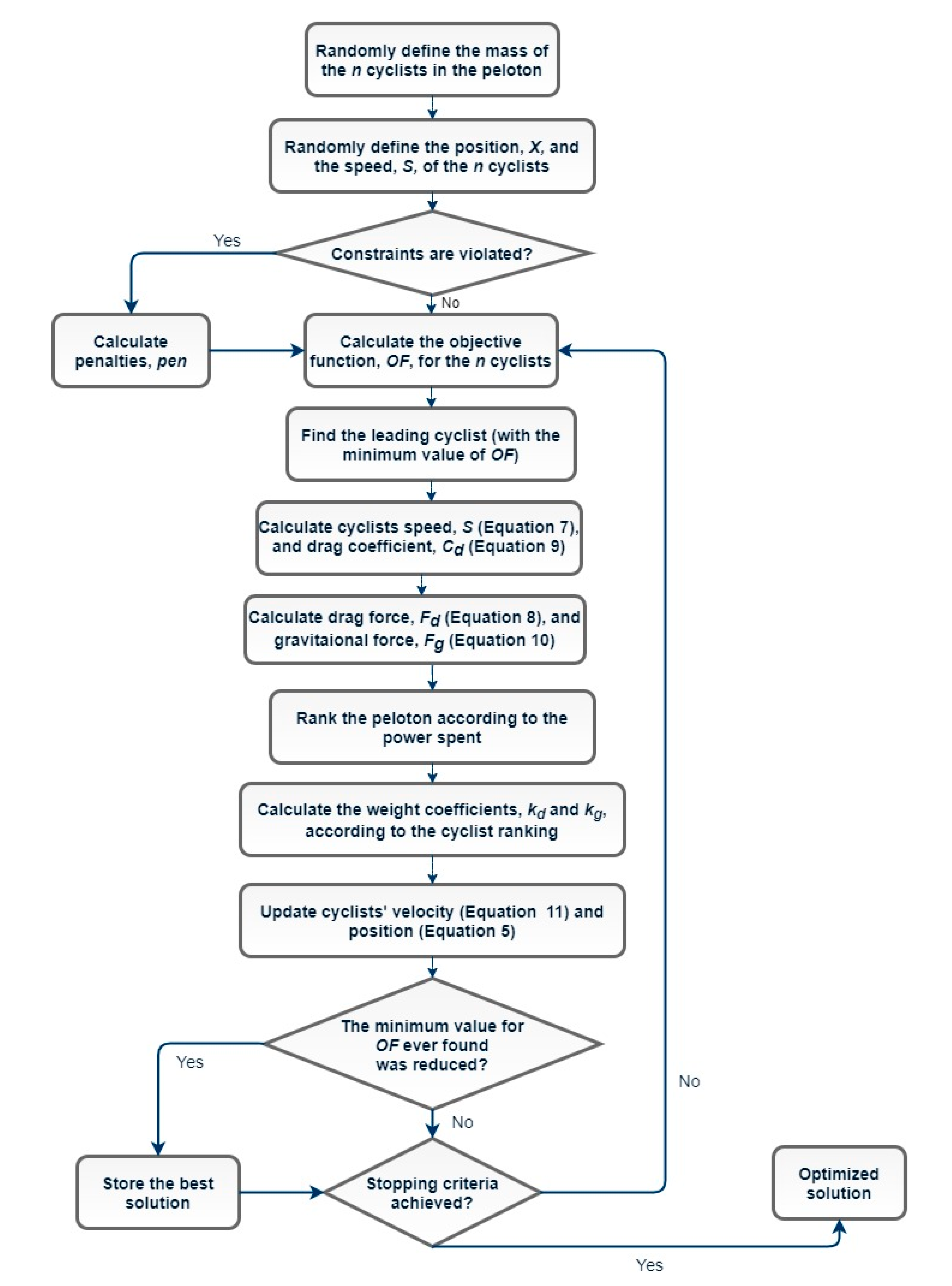
The flowchart in Figure 1 summarizes the GTA optimization process.
2.4. Test Conditions
The GTA algorithm is implemented in Matlab [35], and its source code is available at https://www.mathworks.com/matlabcentral/fileexchange/78922-grand-tour-algorithm-gta.
Four classical metaheuristic algorithms are used for comparison: (i) Particle Swarm Optimization (PSO) [7]; (ii) Simulated Annealing (SA) [8]; (iii) Genetic Algorithm (GA) [32]; and (iv) Harmony Search (HS) [33]. The characteristic parameters of each algorithm, and their general settings used in this study, are presented in Table 1. We chose these algorithms because each belongs to one of the categories in which metaheuristic algorithms are classified [1], because they are, perhaps, the most used algorithms within their categories, and because the authors have used them for several engineering applications in Urban Hydraulics with good results, and have their codes ready.
To evaluate the performance of the five algorithms, each was applied 100 times to fourteen well-known benchmark functions from the literature [36,37] and collections of online of test functions, such as the library GAMS World [38], CUTE [39], and GO Test Problems [40]. In addition, [41] provides an exhaustive list of up to 175 functions. We chose the 14 benchmark fitness functions as a random sample among those used by the optimization community, while having formulas involving an arbitrary number of variables, since we were targeting very high-dimensional problems.
Table 2 shows the name and the equation of each function, the domain considered for the variables, and the minimum value they attained. Let us note here that dimension n was firstly set to 1000 variables, and then to 20,000, a value inspired by human DNA, which may be represented by 20,000 genes [42,43].
Finally, the computer used to run these optimizations had the following characteristics: Acer Aspire A515, Jundiaí/SP – Brazil, Intel Core i5-8265U (8th generation), 1.8 GHz, 8 GB Ram.
3. Results
3.1. Performance
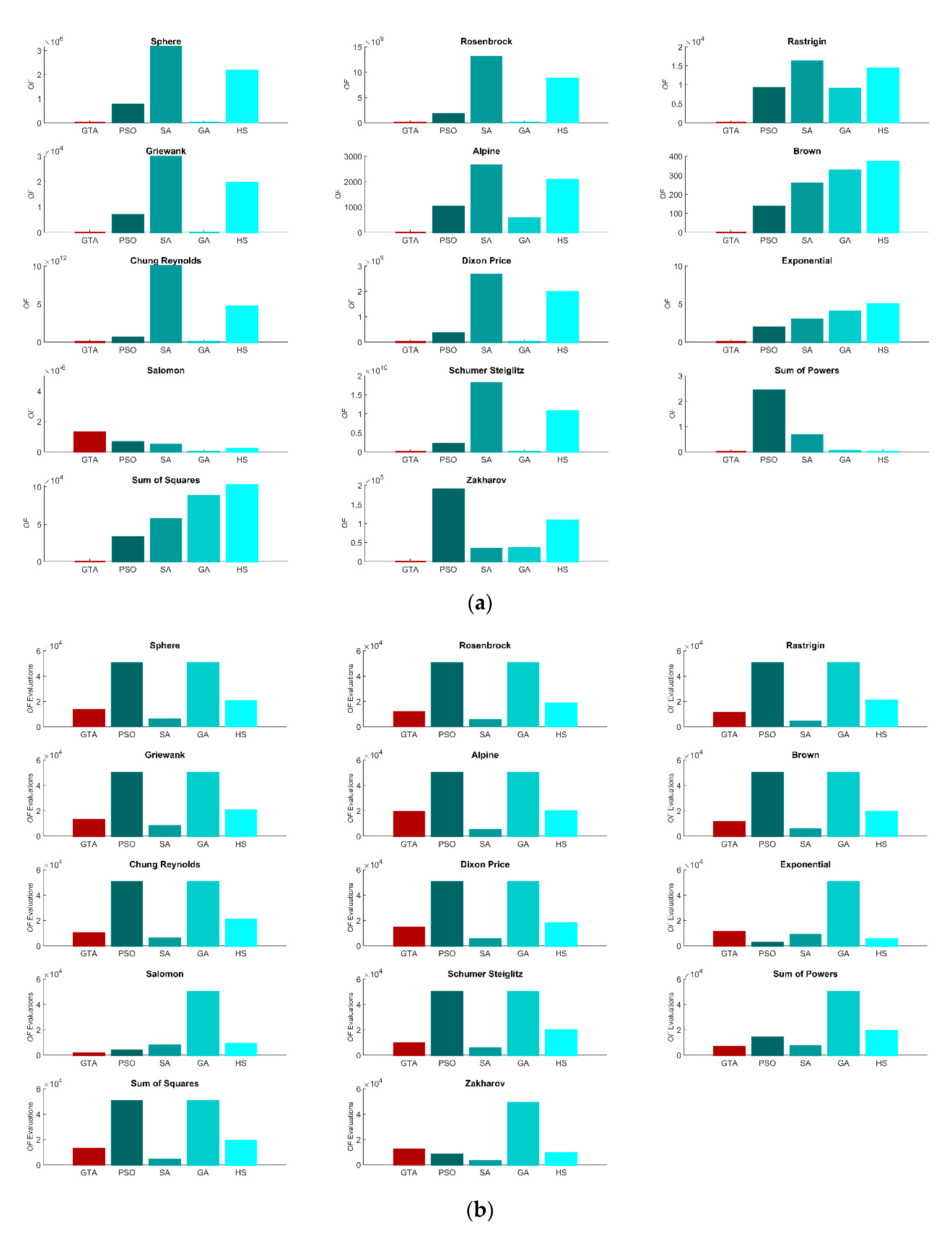
Table 3 summarizes the results of 100 runs for all five algorithms, considering a dimension of 1000 variables. The following parameters are presented: (i) best value found; (ii) mean value; (iii) standard deviation; (iv) success rate, defined as an error less than 10−8 [34]; (v) mean of objective function () evaluations; and (vi) score. Figure 2a,b graphically presents values (ii) and (v), respectively. This score is a parameter considered for the CEC 2017 competition in [44] to compare different optimization algorithms, and is expressed by Equations (12) and (13).
Here, is the optimized value of the run i, is the global minimum, and is the minimum value among the five algorithms for .
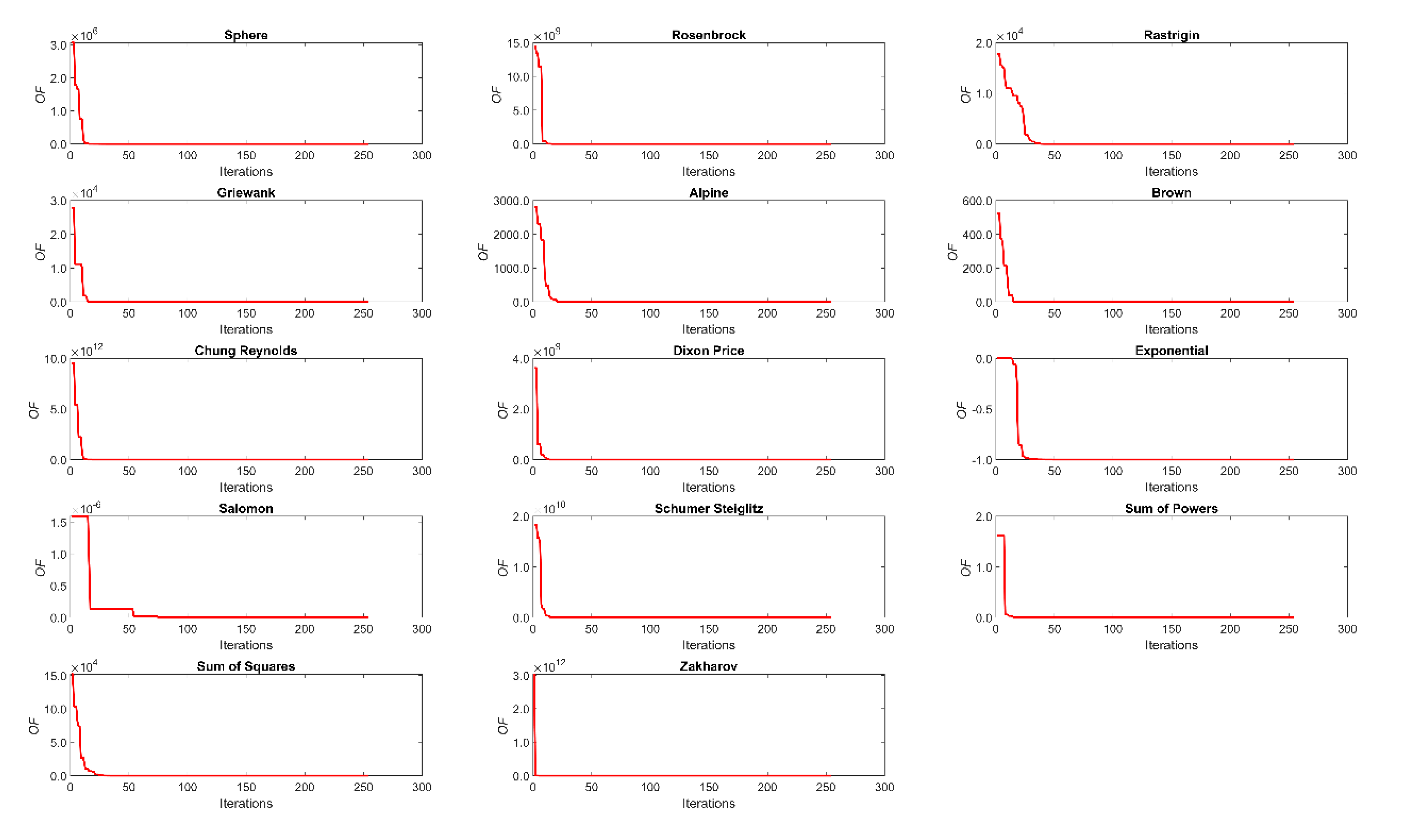
The GTA was the only algorithm to reach the minimum value in eleven of the fourteen benchmarking functions. In addition, in all of the 100 runs, the optimization was a success, yielding an error lower than 10−8. For the Rosenbrock and Dixon Price functions, none of the algorithms achieved the global minimum. However, the GTA was the closest, with a low standard deviation, which indicates the determination of a local minimum. These two functions are well-known examples of very challenging benchmark optimization functions, which have presented many difficulties for all metaheuristics; see, for example [45,46,47], which use different algorithms and report the same difficulty in reaching the global minimum for these functions despite using less than 100 variables. Finally, for the Salomon function, the GTA presents the worst success rate, while GA presents the best one. However, the mean value reached is very close to the global minimum, and the use of more cyclists, or an increase in the maximum number of iterations, could solve this problem. For the other algorithms, only for the function Sum of Powers, this change of settings could lead to a better success rate, since for the other functions, the value found is too far from the global minimum. The reliability of the GTA is also confirmed by its score, which is not the best only for the Salomon function. To evaluate the convergence speed, Figure 3 shows the evolution for each of the benchmarking functions using GTA. It can be seen that a minimum is rapidly achieved, with a finetuning in the following iterations. Comparing the values of the number of evaluations in Table 3 for the Salomon and Sum of Powers functions, where the results of all five algorithms are close, the GTA was the one with the lowest number of evaluations, thus requiring less computational effort.
To finalize the comparison with the classical metaheuristic algorithms, a statistical analysis is performed to evaluate the quality of the solutions, using the Wilcoxon signed-rank test [48] with a 0.05 significance value. Table 4 shows the results of the comparison of GTA with the algorithms. In more than 90% of the solutions, GTA outperformed or equaled the algorithms. The values found for all the comparisons were null. Thus, the performance difference between GTA and those algorithms is significant.
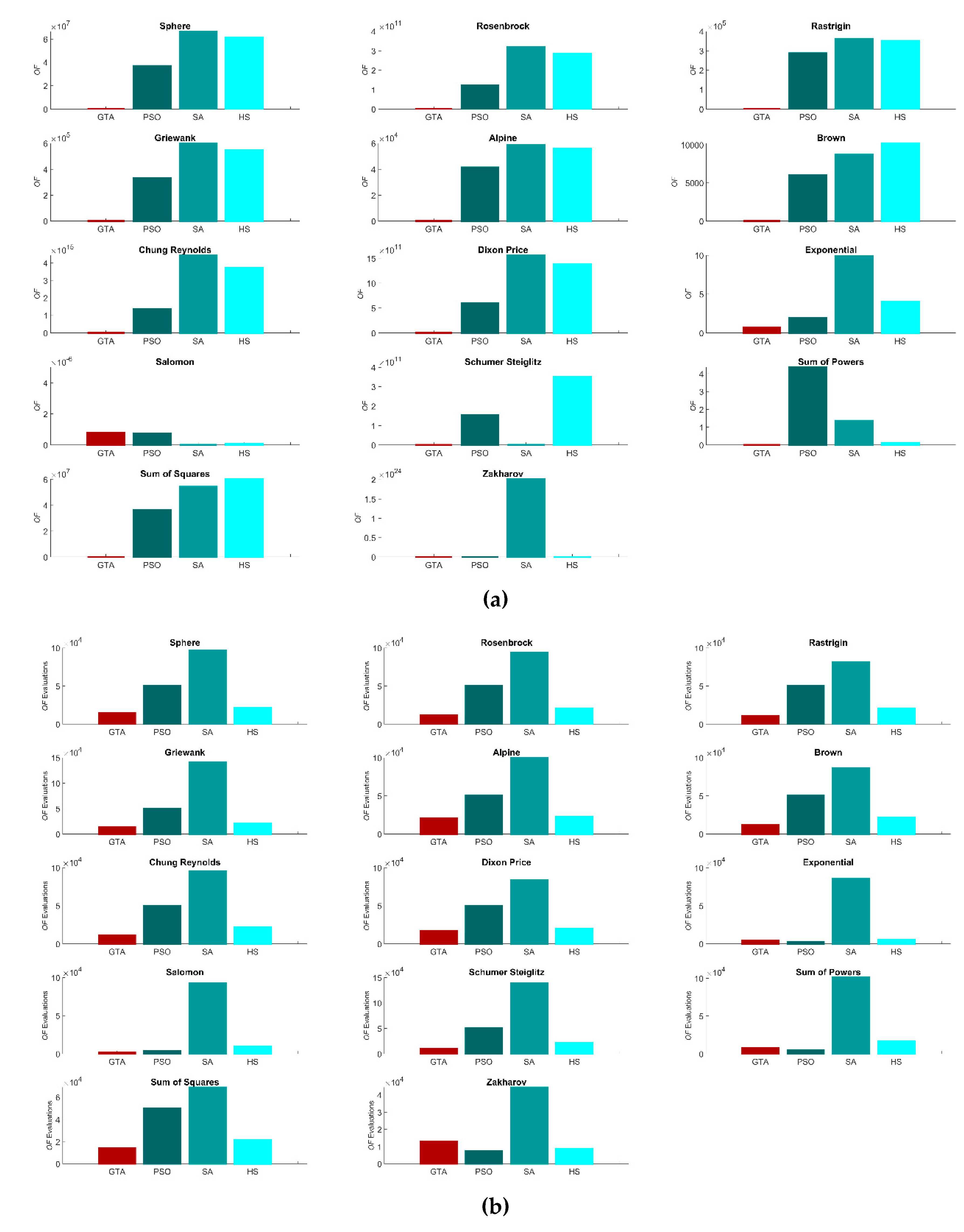
For a final test, GTA was applied once more to the fourteen benchmarking functions, but this time, the dimension was increased to 20,000 variables. As can be seen in Table 5, the results remain similar to those obtained with 1000 variables. The success rates are lower for the Exponential and Sum of Powers functions, but both are still close to the global minimum. The Rosenbrock and Dixon-Price functions again achieve a local minimum, and the Salomon function again yields a low success rate. An additional test for these five functions using 500 cyclists was made to try to reach the global minimum. This procedure was effective for the Exponential, Sum of Powers, and Salomon functions, reaching a 100% success rate, albeit with a significant increase in the number of evaluations (+100–500%). Nevertheless, the GTA was still robust and fast for this highly dimensional analysis. Figure 4 shows the results for GTA and the other metaheuristics for the 20,000-variable problems. It can be observed that SA significantly increased the number of OF evaluations, while all of them reached a higher average OF value in all cases, except for the Salomon function. Let us note that the GA could not be tested in this scenario due to a lack of memory on the computer used.
3.2. Sensitivity Analysis
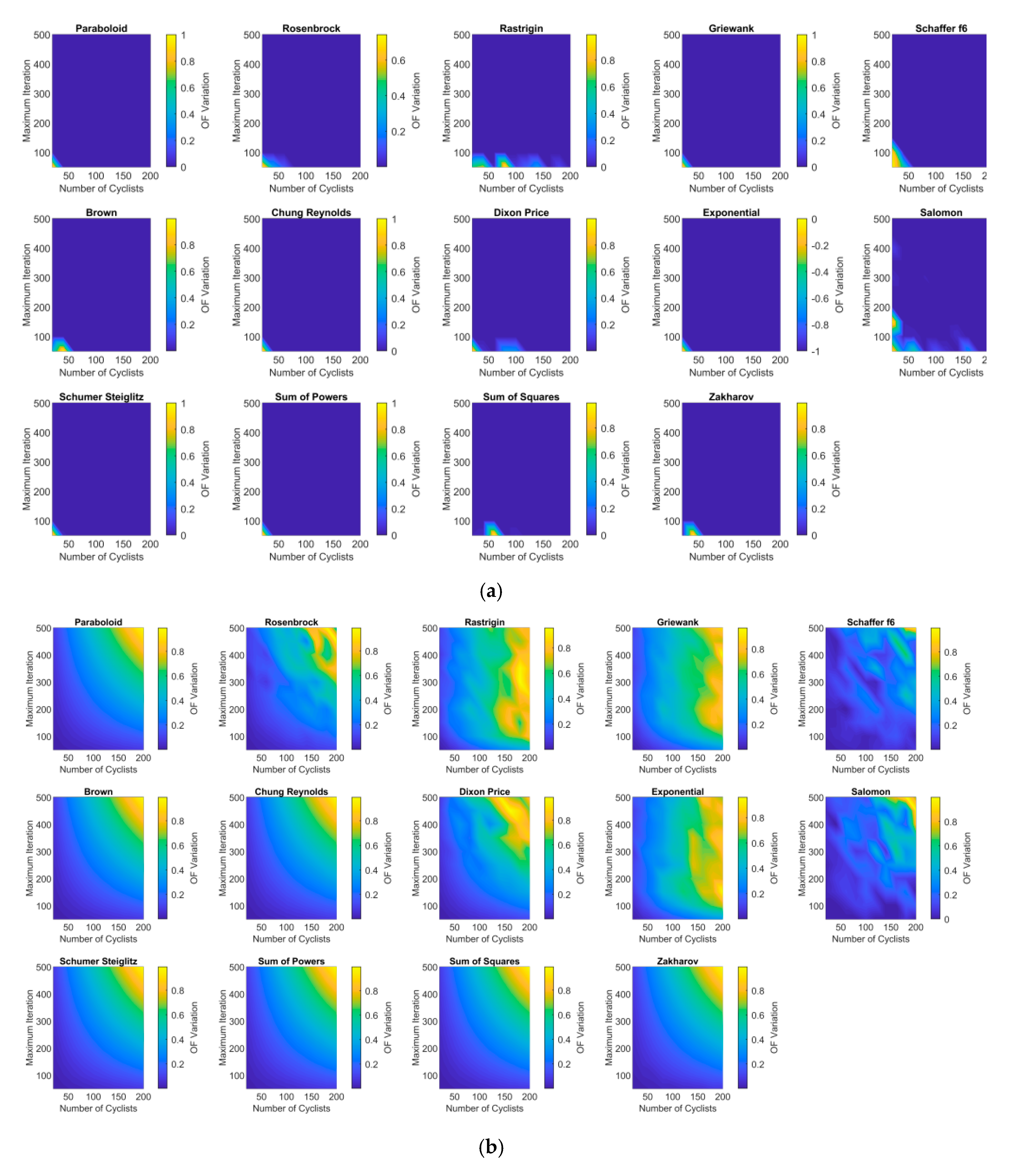
Here, we report three tests, always using 20,000 variables as the functions dimension. The first test is performed to evaluate the relevance of the number of cyclists and the maximum number of iterations in the optimization process. Figure 5a shows that the increase in the numbers of cyclists and maximum number of iterations has no significant influence on the reduction of the objective function. Only a combination of low numbers of cyclists and iterations yielded poor results. As expected, Figure 5b shows an increase of the number of objective function evaluations when both parameters are increased. Therefore, the algorithm yields the best results after extensive searching, but, as observed in Figure 3, with no significant changes. These results agree with those obtained previously, showing that GTA has a fast convergence to a feasible and high-quality solution.
The second sensitivity analysis focused on variations of cyclists’ masses. For this purpose, the minimum and maximum values considered were changed to a range from 25 to 125 kg. The results showed no significant difference. Only when all the cyclists had the same weight, regardless of the value, the optimization became slower and yielded worse results. This lack of randomness hampers the exploration of points near the boundaries, since there are no lightweight cyclists, who are less affected by the gravitational force, to venture closer to the boundaries because of the penalties.
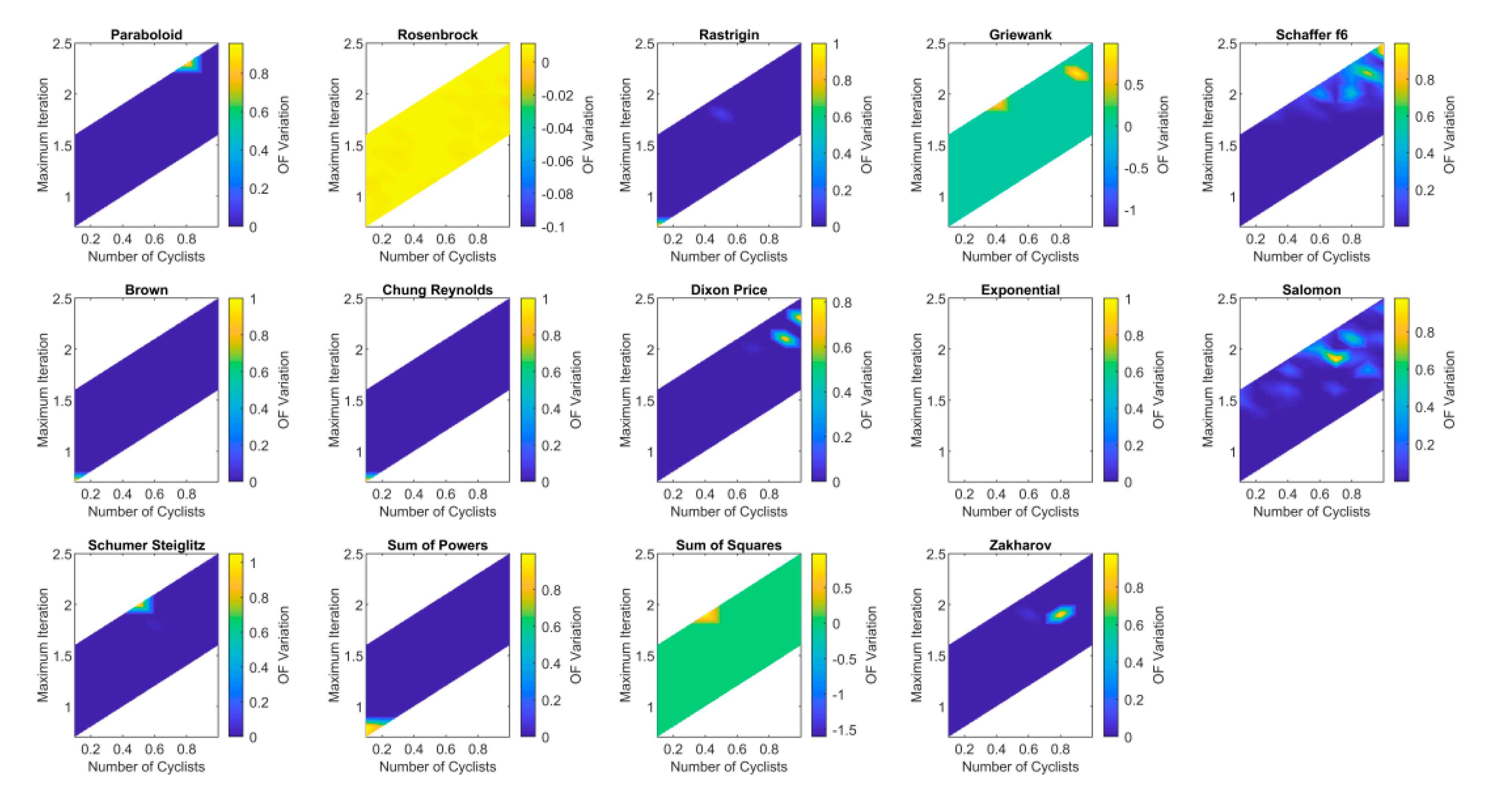
Finally, the score used to calculate the and coefficients of the ranked cyclists according to the power spent in each iteration was evaluated. The best cyclist, or the one who expends the least energy, receives the highest score, while the worst receives the minimum. Figure 6 shows that only with a combination of high values, the results of the objective function got worse. In terms of the number of evaluations of the objective function, no significant difference was observed. In all the analyses made, the GTA presented consistent results despite changes in its parameters. This robustness is very interesting for the user, since there is no need for heavy fine-tuning to adjust the default parameters to obtain the best optimization.
4. Conclusions
As a swarm-based algorithm, GTA exhibits good results in terms of consistency and speed to find the optimal solution for the benchmarking problems considered. GTA performance is clearly superior to that of the classical algorithms used in this paper for comparison, in terms of speed and consistency when functions with a huge (human genome-like) search space (up to 20,000 decision variables) were tested. The great advantage of GTA is its ability to direct the cyclists to search for the fastest path to improve the objective function. At the same time, points with worst objective function values are explored locally, since they may be just a barrier for big improvements. The search for the fastest path has a similar goal as the first derivative, hence its fast convergence, despite the number of cyclists and iterations used. Finally, a sensitivity analysis shows the robustness of GTA, since a change in the main parameters has little impact on the final result. This feature results in a user-friendly algorithm, as there is no need to adjust the default parameters to achieve a good optimization. Therefore, the three most desirable aspects for an optimization algorithm, i.e., ease of implementation, speed of convergence, and reliability, had good results, confirming the expected improvements of GTA. Having presented the GTA, our target is now to develop it further in several directions so that it may also become efficient with real-world problems; this development will include constrained optimization, multi-objective optimization, and the development of mechanisms for GTA to dynamically accommodate to changing fitness functions.
Author Contributions
Conceptualization, G.M. and B.B.; methodology, G.M., B.B. and J.I.; software, G.M.; investigation, G.M., B.B., J.I. and E.L.J.; writing, G.M., B.B.; review and editing, G.M., B.B., J.I. and E.L.J. All authors have read and agreed to the published version of the manuscript.
Funding
This research received no external funding.
Conflicts of Interest
The authors declare no conflict of interest
References
- Mohamed, A.W.; Hadi, A.A.; Mohamed, A.K. Gaining-sharing knowledge based algorithm for solving optimization problems: A novel nature-inspired algorithm. Int. J. Mach. Learn. Cyb. 2019, 11, 1501–1529. [Google Scholar]
- Mirjalili, S.; Lewis, A. The whale optimization algorithm. Adv. Eng. Soft. 2016, 95, 51–67. [Google Scholar] [CrossRef]
- Chatterjee, A.; Siarry, P. Nonlinear inertia weight variation for dynamic adaptation in particle swarm optimization. Comput. Oper. Res. 2006, 33, 859–871. [Google Scholar] [CrossRef]
- Dorigo, M.; Blum, C. Ant colony optimization theory: A survey. Theor. Comput. Sci. 2005, 344, 243–278. [Google Scholar] [CrossRef]
- Karaboga, D.; Basturk, B. A powerful and efficient algorithm for numerical function optimization: Artificial bee colony (ABC) algorithm. J. Global Optim. 2007, 39, 459–471. [Google Scholar] [CrossRef]
- Gandomi, A.H.; Yang, X.S.; Alavi, A.H. Cuckoo search algorithm: A metaheuristic approach to solve structural optimization problems. Eng. Comput. 2013, 29, 17–35. [Google Scholar] [CrossRef]
- Kennedy, J.; Eberhart, R. Particle swarm optimization (PSO). In Proceedings of the IEEE Intern Conf Neural Net, Perth, Australia, 27 November–1 December 1995; pp. 1942–1948. [Google Scholar]
- Kirkpatrick, S.; Gelatt, C.D.; Vecchi, M.P. Optimization by simulated annealing. Science 1983, 220, 671–680. [Google Scholar] [CrossRef]
- Gonzalez-Fernandez, Y.; Chen, S. Leaders and followers—A new metaheuristic to avoid the bias of accumulated information. In Proceedings of the 2015 IEEE Congress on Evolutionary Computation (CEC), Sendai, Japan, 25–28 May 2015; pp. 776–783. [Google Scholar]
- Parsopoulos, K.E.; Vrahatis, M.N. Particle swarm optimization method for constrained optimization problems. Intell. Tech. Theory Appl. New Trends Intell. Tech. 2002, 76, 214–220. [Google Scholar]
- Wu, Z.Y.; Simpson, A.R. A self-adaptive boundary search genetic algorithm and its application to water distribution systems. J. Hydr. Res. 2002, 40, 191–203. [Google Scholar] [CrossRef] [Green Version]
- Trelea, I.C. The particle swarm optimization algorithm: Convergence analysis and parameter selection. Inf. Process Lett. 2003, 85, 317–325. [Google Scholar] [CrossRef]
- Brentan, B.; Meirelles, G.; Luvizotto, E., Jr.; Izquierdo, J. Joint operation of pressure-reducing valves and pumps for improving the efficiency of water distribution systems. J. Water Res. Plan. Manag. 2018, 144, 04018055. [Google Scholar] [CrossRef] [Green Version]
- Freire, R.Z.; Oliveira, G.H.; Mendes, N. Predictive controllers for thermal comfort optimization and energy savings. Ener. Build. 2008, 40, 1353–1365. [Google Scholar] [CrossRef]
- Banga, J.R.; Seider, W.D. Global optimization of chemical processes using stochastic algorithms. In State of the Art in Global Optimization; Springer: Boston, MA, USA, 1996; pp. 563–583. [Google Scholar]
- Waziruddin, S.; Brogan, D.C.; Reynolds, P.F. The process for coercing simulations. In Proceedings of the 2003 Fall Simulation Interoperability Workshop, Orlando, FL, USA, 14–19 September 2003. [Google Scholar]
- Carnaham, J.C.; Reynolds, P.F.; Brogan, D.C. Visualizing coercible simulations. In Proceedings of the 2004 Winter Simulation Conference, Washington, DC, USA, 5–8 December 2004; Volume 1. [Google Scholar]
- Bollinger, A.; Evins, R. Facilitating model reuse and integration in an urban energy simulation platform. Proc. Comput. Sci. 2015, 51, 2127–2136. [Google Scholar] [CrossRef] [Green Version]
- Yang, Y.; Chui, T.F.M. Developing a Flexible Simulation-Optimization Framework to Facilitate Sustainable Urban Drainage Systems Designs through Software Reuse. In Proceedings of the International Conference on Software and Systems Reuse, Cincinnati, OH, USA, 26–28 June 2019. [Google Scholar] [CrossRef]
- Yazdani, C.; Nasiri, B.; Azizi, R.; Sepas-Moghaddam, A.; Meybodi, M.R. Optimization in Dynamic Environments Utilizing a Novel Method Based on Particle Swarm Optimization. Int. J. Artif. Intel. 2013, 11, A13. [Google Scholar]
- Wang, Z.-J.; Zhan, Z.-H.; Du, K.-J.; Yu, Z.-W.; Zhang, J. Orthogonal learning particle swarm optimization with variable relocation for dynamic optimization. In Proceedings of the 2016 IEEE Congress on Evolutionary Computation (CEC), Vancouver, BC, Canada, 24–29 July 2016. [Google Scholar] [CrossRef]
- Mavrovouniotis, M.; Lib, C.; Yang, S. A survey of swarm intelligence for dynamic optimization: Algorithms and applications. Swarm Evol. Comput. 2017, 33, 1–17. [Google Scholar] [CrossRef] [Green Version]
- Gore, R.; Reynolds, P.F.; Tang, L.; Brogan, D.C. Explanation exploration: Exploring emergent behavior. In Proceedings of the 21st International Workshop on Principles of Advanced and Distributed Simulation (PADS’07), San Diego, CA, USA, 12–15 June 2007; IEEE: Washington, DC, USA, June 2007. [Google Scholar] [CrossRef] [Green Version]
- Gore, R.; Reynolds, P.F. Applying causal inference to understand emergent behavior. In Proceedings of the 2008 Winter Simulation Conference, Miami, FL, USA, 7–10 December 2008; IEEE: Washington, DC, USA, December 2008. [Google Scholar] [CrossRef]
- Kim, V. A Design Space Exploration Method for Identifying Emergent Behavior in Complex Systems. Ph.D. Thesis, Georgia Institute of Technology, Atlanta, GA, USA, December 2016. [Google Scholar]
- Hybinette, M.; Fujimoto, R.M. Cloning parallel simulations. ACM Trans. Model. Comput. Simul. (TOMACS) 2001, 11, 378–407. [Google Scholar] [CrossRef]
- Hybinette, M.; Fujimoto, R. Cloning: A novel method for interactive parallel simulation. In Proceedings of the WSC97: 29th Winter Simulation Conference, Atlanta, GA, USA, 7–10 December 1997; pp. 444–451. [Google Scholar] [CrossRef]
- Chen, D.; Turner, S.J.; Cai, W.; Gan, B.P. Low MYH Incremental HLA-Based Distributed Simulation Cloning. In Proceedings of the 2004 Winter Simulation Conference, Washington, DC, USA, 5–8 December 2004; IEEE: Washington, DC, USA, December 2004. [Google Scholar] [CrossRef]
- Li, Z.; Wang, W.; Yan, Y.; Li, Z. PS–ABC: A hybrid algorithm based on particle swarm and artificial bee colony for high-dimensional optimization problems. Exp. Syst. Appl. 2015, 42, 8881–8895. [Google Scholar] [CrossRef]
- Montalvo, I.; Izquierdo, J.; Pérez-García, R.; Herrera, M. Water distribution system computer-aided design by agent swarm optimization. Comput. Aided Civil Infrastr. Eng. 2014, 29, 433–448. [Google Scholar] [CrossRef]
- Maringer, D.G. Portfolio Management with Heuristic Optimization; Springer Science & Business Media: Boston, MA, USA, 2006. [Google Scholar] [CrossRef] [Green Version]
- Holland, J.H. Adaptation in Natural and Artificial Systems: An Introductory Analysis with Applications to Biology, Control, and Artificial Intelligence; MIT Press: Cambridge, MA, USA, 1992. [Google Scholar]
- Geem, Z.W.; Kim, J.H.; Loganathan, G.V. A new heuristic optimization algorithm: Harmony search. Simulation 2001, 76, 60–68. [Google Scholar] [CrossRef]
- Blocken, B.; van Druenen, T.; Toparlar, Y.; Malizia, F.; Mannion, P.; Andrianne, T.; Marchal, T.; Maas, G.J.; Diepens, J. Aerodynamic drag in cycling pelotons: New insights by CFD simulation and wind tunnel testing. J. Wind Eng. Ind. Aerod. 2018, 179, 319–337. [Google Scholar] [CrossRef]
- MATLAB 2018; The MathWorks, Inc.: Natick, MA, USA, 2018.
- Clerc, M.; Kennedy, J. The particle swarm-explosion, stability, and convergence in a multidimensional complex space. IEEE Trans. Evol. Comput. 2002, 6, 58–73. [Google Scholar] [CrossRef] [Green Version]
- Eberhart, R.C.; Shi, Y. Comparing inertia weights and constriction factors in particle swarm optimization. In Proceedings of the 2000 Congress on Evolutionary Computation—CEC00 (Cat. No.00TH8512), La Jolla, CA, USA, 16–19 July 2000; Volume 1, pp. 84–88. [Google Scholar]
- GAMS World, GLOBAL Library. Available online: http://www.gamsworld.org/global/globallib.html (accessed on 29 April 2020).
- Gould, N.I.M.; Orban, D.; Toint, P.L. CUTEr, A Constrained and Un-Constrained Testing Environment, Revisited. Available online: http://cuter.rl.ac.uk/cuter-www/problems.html (accessed on 29 April 2020).
- GO Test Problems. Available online: http://www-optima.amp.i.kyoto-u.ac.jp/member/student/hedar/Hedar_files/TestGO.htm (accessed on 29 April 2020).
- Jamil, M.; Yang, X.S. A literature survey of benchmark functions for global optimisation problems. Int. J. Math. Model. Num. Optim. 2013, 4, 150–194. [Google Scholar] [CrossRef] [Green Version]
- Sharma, G. The Human Genome Project and its promise. J. Indian College Cardiol. 2012, 2, 1–3. [Google Scholar] [CrossRef]
- Li, W. On parameters of the human genome. J. Theor. Biol. 2011, 288, 92–104. [Google Scholar] [CrossRef]
- Awad, N.H.; Ali, M.Z.; Liang, J.J.; Qu, B.Y.; Suganthan, P.N. Problem Definitions and Evaluation Criteria for the CEC 2017 Special Session and Competition on Single Objective Bound Constrained Real-Parameter Numerical Optimization; Technical Report; Nanyang Technological University: Singapore, November 2016. [Google Scholar]
- Hughes, M.; Goerigk, M.; Wright, M. A largest empty hypersphere metaheuristic for robust optimisation with implementation uncertainty. Comput. Oper. Res. 2019, 103, 64–80. [Google Scholar] [CrossRef]
- Zaeimi, M.; Ghoddosian, A. Color harmony algorithm: An art-inspired metaheuristic for mathematical function optimization. Soft Comput. 2020, 24, 12027–12066. [Google Scholar] [CrossRef]
- Singh, G.P.; Singh, A. Comparative Study of Krill Herd, Firefly and Cuckoo Search Algorithms for Unimodal and Multimodal Optimization. J. Intel. Syst. App. 2014, 2, 26–37. [Google Scholar] [CrossRef]
- Taheri, S.M.; Hesamian, G. A generalization of the Wilcoxon signed-rank test and its applications. Stat. Papers 2013, 54, 457–470. [Google Scholar] [CrossRef]
Figure 1.
Flowchart of the Grand Tour Algorithm.

Figure 2.
Results of 100 runs with 1000 variables: (a) OF value average; (b) OF evaluations average.
Figure 2.
Results of 100 runs with 1000 variables: (a) OF value average; (b) OF evaluations average.

Figure 3.
GTA Objective function evolution for the fourteen benchmark functions.

Figure 4.
Results of 100 runs with 20,000 variables: (a) OF value average; (b) OF evaluations average.
Figure 4.
Results of 100 runs with 20,000 variables: (a) OF value average; (b) OF evaluations average.

Figure 5.
Sensitivity analysis for the number of cyclists and the maximum number of iterations: (a) Objective function variation; (b) Number of objective function evaluations.
Figure 5.
Sensitivity analysis for the number of cyclists and the maximum number of iterations: (a) Objective function variation; (b) Number of objective function evaluations.

Figure 6.
Sensitivity analysis for the score of parameters and .


Table 1.
Optimization algorithms’ settings.
| Algorithm | Settings |
|---|---|
| GTA | Drag and Gravitational Coefficients = range from 0.5 to 1.0 |
| PSO | Cognitive and Social Coefficients = 1.49 Inertia coefficient = varying from 0.1 to 1.1, linearly, |
| SA | Initial Temperature = 100 °C Reanneling Interval = 100 |
| GA | Crossover Fraction = 0.8 Elite Count = 0.05 Mutation rate = 0.01 |
| HS | Harmony Memory Considering Rate = 0.8 Pitching Adjust Rate = 0.1 |
| General | Maximum iterations = 500 Population Size = 100 Tolerance = 10−12 Maximum Stall Iteration = 20 |
Table 2.
Benchmarking Functions.
| Function | Equation | Global Minimum | |
|---|---|---|---|
| Sphere | 0 | ||
| Rosenbrock | 0 | ||
| Rastrigin | 0 | ||
| Griewank | 0 | ||
| Alpine | 0 | ||
| Brown | 0 | ||
| Chung Reynolds | 0 | ||
| Dixon Price | 0 | ||
| Exponential | 0 | ||
| Salomon | 0 | ||
| Schumer Steiglitz | 0 | ||
| Sum of Powers | 0 | ||
| Sum of Squares | 0 | ||
| Zakharov | 0 |
Table 3.
Results of 100 runs with 1000 variables.
| Function | Sphere | Rosenbrock | Rastrigin | Griewank | Alpine | Brown | Chung Reynolds | Dixon Price | Exponential | Salomon | Schumer Steiglitz | Sum of Powers | Sum of squares | Zakharov | |
|---|---|---|---|---|---|---|---|---|---|---|---|---|---|---|---|
| Best | GTA | 4.4 × 10⁻¹⁸ | 9.9 × 10² | 0.0 × 100 | 0.0 × 100 | 1.6 × 10⁻¹⁵ | 8.9 × 10⁻¹⁸ | 5.0 × 10⁻²³ | 1.0 × 100 | 0.0E × 100 | 6.7 × 10⁻¹⁰ | 1.4 × 10⁻²³ | 1.3 × 10⁻²² | 2.4 × 10⁻¹⁸ | 1.3 × 10⁻¹⁷ |
| PSO | 6.4 × 10⁵ | 1.3 × 10⁹ | 8.4 × 10³ | 5.8 × 10³ | 9.0 × 10² | 1.1 × 10² | 3.9 × 10¹¹ | 2.5 × 10⁸ | 1.0 × 100 | 2.5 × 10⁻¹² | 1.5 × 10⁹ | 1.1 × 100 | 2.6 × 10⁴ | 2.4 × 10⁴ | |
| SA | 2.9 × 10⁶ | 1.1 × 10¹⁰ | 1.5 × 10⁴ | 2.7 × 10⁴ | 2.4 × 10³ | 2.1 × 10² | 8.7 × 10¹² | 2.2 × 10⁹ | 1.0 × 100 | 1.0 × 10⁻¹⁰ | 1.6 × 10¹⁰ | 6.4 × 10⁻² | 4.5 × 10⁴ | 3.1 × 10⁴ | |
| GA | 8.2 × 10² | 2.6 × 10⁵ | 8.3 × 10³ | 1.1 × 100 | 5.2 × 10² | 2.9 × 10² | 6.8 × 10⁵ | 3.8 × 10⁶ | 1.0 × 100 | 0.0 × 100 | 2.0 × 10³ | 5.3 × 10⁻³ | 7.7 × 10⁴ | 1.0 × 10³ | |
| HS | 2.1 × 10⁶ | 7.9 × 10⁹ | 1.4 × 10⁴ | 1.8 × 10⁴ | 2.0 × 10³ | 3.6 × 10² | 4.2 × 10¹² | 1.8 × 10⁹ | 1.0 × 100 | 1.4 × 10⁻¹³ | 1.0 × 10¹⁰ | 2.4 × 10⁻³ | 9.5 × 10⁴ | 3.0 × 10⁴ | |
| Mean | GTA | 2.3 × 10⁻¹⁵ | 1.0 × 10³ | 0.0 × 100 | 1.6 × 10⁻¹⁵ | 6.9 × 10⁻¹⁴ | 3.3 × 10⁻¹⁵ | 8.1 × 10⁻¹⁸ | 1.0 × 100 | 0.0 × 100 | 1.3 × 10⁻⁶ | 1.3 × 10⁻¹⁷ | 1.5 × 10⁻¹⁶ | 3.4 × 10⁻¹⁵ | 1.7 × 10⁻¹⁵ |
| PSO | 7.5 × 10⁵ | 1.7 × 10⁹ | 9.1 × 10³ | 6.9 × 10³ | 1.0 × 10³ | 1.4 × 10² | 5.9 × 10¹¹ | 3.6 × 10⁸ | 1.0 × 100 | 6.4 × 10⁻⁷ | 2.1 × 10⁹ | 2.4 × 100 | 3.3 × 10⁴ | 1.9 × 10⁵ | |
| SA | 3.2 × 10⁶ | 1.3 × 10¹⁰ | 1.6 × 10⁴ | 3.0 × 10⁴ | 2.6 × 10³ | 2.6 × 10² | 1.0 × 10¹³ | 2.6 × 10⁹ | 1.0 × 100 | 4.5 × 10⁻⁷ | 1.8 × 10¹⁰ | 6.5 × 10⁻¹ | 5.7 × 10⁴ | 3.4 × 10⁴ | |
| GA | 9.2 × 10² | 3.1 × 10⁵ | 8.9 × 10³ | 1.2 × 100 | 5.6 × 10² | 3.2 × 10² | 8.5 × 10⁵ | 5.0 × 10⁶ | 1.0 × 100 | 7.7 × 10⁻¹³ | 2.5 × 10³ | 4.0 × 10⁻² | 8.8 × 10⁴ | 3.5 × 10⁴ | |
| HS | 2.2 × 10⁶ | 8.6 × 10⁹ | 1.4 × 10⁴ | 1.9 × 10⁴ | 2.1 × 10³ | 3.7 × 10² | 4.7 × 10¹² | 2.0 × 10⁹ | 1.0 × 100 | 1.9 × 10⁻⁷ | 1.1 × 10¹⁰ | 1.2 × 10⁻² | 1.0 × 10⁵ | 1.1 × 10⁵ | |
| Standard deviation | GTA | 5.3 × 10⁻¹⁵ | 9.1 × 10⁻¹ | 0.0 × 100 | 3.4 × 10⁻¹⁵ | 9.3 × 10⁻¹⁴ | 1.3 × 10⁻¹⁴ | 2.9 × 10⁻¹⁷ | 4.3 × 10⁻⁶ | 0.0 × 100 | 3.2 × 10⁻⁶ | 6.5 × 10⁻¹⁷ | 5.3 × 10⁻¹⁶ | 8.7 × 10⁻¹⁵ | 4.4 × 10⁻¹⁵ |
| PSO | 5.1 × 10⁴ | 1.9 × 10⁸ | 3.2 × 10² | 5.1 × 10² | 4.5 × 101 | 9.7 × 100 | 9.4 × 10¹⁰ | 4.7 × 10⁷ | 3.0 × 10–38 | 1.7 × 10⁻⁶ | 2.8 × 10⁸ | 4.6 × 10⁻¹ | 2.7 × 10³ | 1.2 × 10⁶ | |
| SA | 8.9 × 10⁴ | 5.4 × 10⁸ | 4.4 × 10² | 8.1 × 10² | 8.6 × 101 | 2.3 × 101 | 5.8 × 10¹¹ | 1.5 × 10⁸ | 1.4 × 10–36 | 2.6 × 10⁻⁶ | 7.7 × 10⁸ | 3.9 × 10⁻¹ | 5.2 × 10³ | 1.3 × 10³ | |
| GA | 4.4 × 101 | 2.6 × 10⁴ | 2.6 × 10² | 3.8 × 10⁻² | 1.7 × 101 | 1.2 × 101 | 7.4 × 10⁴ | 5.7 × 10⁵ | 2.1 × 10–39 | 5.3 × 10⁻¹² | 2.9 × 10² | 3.7 × 10⁻² | 4.5 × 10³ | 3.3 × 10⁴ | |
| HS | 3.7 × 10⁴ | 2.4 × 10⁸ | 1.6 × 10² | 4.1 × 10² | 3.2 × 101 | 7.2 × 100 | 1.9 × 10¹¹ | 6.2 × 10⁷ | 3.0 × 10–49 | 6.8 × 10⁻⁷ | 2.7 × 10⁸ | 6.2 × 10⁻³ | 2.5 × 10³ | 3.8 × 10⁵ | |
| Success rate | GTA | 100 | 0 | 100 | 100 | 100 | 100 | 100 | 0 | 100 | 12 | 100 | 100 | 100 | 100 |
| PSO | 0 | 0 | 0 | 0 | 0 | 0 | 0 | 0 | 0 | 18 | 0 | 0 | 0 | 0 | |
| SA | 0 | 0 | 0 | 0 | 0 | 0 | 0 | 0 | 0 | 20 | 0 | 0 | 0 | 0 | |
| GA | 0 | 0 | 0 | 0 | 0 | 0 | 0 | 0 | 0 | 100 | 0 | 0 | 0 | 0 | |
| HS | 0 | 0 | 0 | 0 | 0 | 0 | 0 | 0 | 0 | 31 | 0 | 0 | 0 | 0 | |
| evaluations | GTA | 13,401 | 11,605 | 10,920 | 12,686 | 19,352 | 11,234 | 9983 | 14,314 | 10,764 | 1701 | 9273 | 6757 | 12,573 | 11,933 |
| PSO | 50,100 | 50,100 | 50,100 | 50,100 | 50,100 | 50,100 | 50,100 | 50,100 | 2200 | 3874 | 50,100 | 14,016 | 50,100 | 8064 | |
| SA | 5562 | 5132 | 4272 | 8002 | 5142 | 5632 | 5532 | 5002 | 8342 | 7622 | 5352 | 6972 | 4002 | 3032 | |
| GA | 50,100 | 50,100 | 50,100 | 50,100 | 50,100 | 50,100 | 50,100 | 50,100 | 50,100 | 50,100 | 50,100 | 50,100 | 50,100 | 48,817 | |
| HS | 19,956 | 18,340 | 20,824 | 20,365 | 19,457 | 19,251 | 20,315 | 17,935 | 5010 | 8965 | 19,430 | 19,385 | 18,770 | 8976 | |
| Score | GTA | 1.000 | 1.000 | 1.000 | 1.000 | 1.000 | 1.000 | 1.000 | 1.000 | 1.000 | 0.000 | 1.000 | 1.000 | 1.000 | 1.000 |
| PSO | 0.000 | 0.000 | 0.000 | 0.000 | 0.000 | 0.000 | 0.000 | 0.000 | 0.000 | 0.000 | 0.000 | 0.000 | 0.000 | 0.000 | |
| SA | 0.000 | 0.000 | 0.000 | 0.000 | 0.000 | 0.000 | 0.000 | 0.000 | 0.000 | 0.000 | 0.000 | 0.000 | 0.000 | 0.000 | |
| GA | 0.000 | 0.003 | 0.000 | 0.000 | 0.000 | 0.000 | 0.000 | 0.000 | 0.000 | 1.000 | 0.000 | 0.000 | 0.000 | 0.000 | |
| HS | 0.000 | 0.000 | 0.000 | 0.000 | 0.000 | 0.000 | 0.000 | 0.000 | 0.000 | 0.000 | 0.000 | 0.000 | 0.000 | 0.000 | |
Table 4.
Comparison of results between GTA and classical algorithms.
| Comparison | GTA vs PSO | GTA vs SA | GTA vs AG | GTA vs HS |
|---|---|---|---|---|
| GTA [%] | 95.65 | 94.96 | 92.86 | 94.54 |
| Algorithm [%] | 4.12 | 4.74 | 6.29 | 5.06 |
| Equal [%] | 0.24 | 0.31 | 0.86 | 0.39 |
| -value | 0 | 0 | 0 | 0 |
Table 5.
Results of 100 runs with 20,000 variables using GTA.
| Function | Best | Standard Deviation | Sucess Rate | ||
|---|---|---|---|---|---|
| Sphere | 2.14 × 10⁻¹⁸ | 1.88 × 10⁻¹⁵ | 3.73 × 10⁻¹⁵ | 100 | 14,328 |
| Rosenbrock | 1.99 × 10⁴ | 2.00 × 10⁴ | 2.53 × 101 | 0 | 11,195 |
| Rastrigin | 0.00 × 100 | 0.00 × 100 | 0.00 × 100 | 100 | 10,488 |
| Griewank | 0.00 × 100 | 1.34 × 10⁻¹⁵ | 2.51 × 10⁻¹⁵ | 100 | 13,080 |
| Alpine | 2.44 × 10⁻¹⁵ | 7.19 × 10⁻¹⁴ | 7.22 × 10⁻¹⁴ | 100 | 20,593 |
| Brown | 1.84 × 10⁻¹⁸ | 2.29 × 10⁻¹⁵ | 5.34 × 10⁻¹⁵ | 100 | 12,007 |
| Chung Reynolds | 1.69 × 10⁻²⁴ | 2.52 × 10⁻¹⁷ | 1.32 × 10⁻¹⁶ | 100 | 10,947 |
| Dixon Price | 1.00 × 100 | 1.00 × 100 | 1.20 × 10⁻⁸ | 0 | 16,782 |
| Exponential | 0.00 × 100 | 7.40 × 10⁻¹ | 4.41 × 10⁻¹ | 26 | 4132 |
| Salomon | 2.96 × 10⁻¹⁰ | 7.95 × 10⁻⁷ | 1.76 × 10⁻⁶ | 12 | 1518 |
| Schumer Steiglitz | 1.20 × 10⁻²² | 1.00 × 10⁻¹⁷ | 3.86 × 10⁻¹⁷ | 100 | 9657 |
| Sum of Powers | 3.09 × 10⁻²¹ | 1.16 × 10⁻³ | 1.02 × 10⁻² | 97 | 8052 |
| Sum of Squares | 1.83 × 10⁻¹⁸ | 2.46 × 10⁻¹⁵ | 6.20 × 10⁻¹⁵ | 100 | 14,238 |
| Zakharov | 5.92 × 10⁻¹⁹ | 2.11 × 10⁻¹⁵ | 4.47 × 10⁻¹⁵ | 100 | 13,075 |
© 2020 by the authors. Licensee MDPI, Basel, Switzerland. This article is an open access article distributed under the terms and conditions of the Creative Commons Attribution (CC BY) license (http://creativecommons.org/licenses/by/4.0/).
Share and Cite
MDPI and ACS Style
Meirelles, G.; Brentan, B.; Izquierdo, J.; Luvizotto, E., Jr. Grand Tour Algorithm: Novel Swarm-Based Optimization for High-Dimensional Problems. Processes 2020, 8, 980. https://0-doi-org.brum.beds.ac.uk/10.3390/pr8080980
AMA Style
Meirelles G, Brentan B, Izquierdo J, Luvizotto E Jr. Grand Tour Algorithm: Novel Swarm-Based Optimization for High-Dimensional Problems. Processes. 2020; 8(8):980. https://0-doi-org.brum.beds.ac.uk/10.3390/pr8080980
Chicago/Turabian StyleMeirelles, Gustavo, Bruno Brentan, Joaquín Izquierdo, and Edevar Luvizotto, Jr. 2020. "Grand Tour Algorithm: Novel Swarm-Based Optimization for High-Dimensional Problems" Processes 8, no. 8: 980. https://0-doi-org.brum.beds.ac.uk/10.3390/pr8080980
Note that from the first issue of 2016, this journal uses article numbers instead of page numbers. See further details here.