
Combining Kinetic and Constraint-Based Modelling to Better Understand Metabolism Dynamics


1
Université Paris-Saclay, CNRS, Laboratoire Interdisciplinaire des Sciences du Numérique, 91400 Orsay, France
2
Université Paris-Saclay, INRAE, MaIAGE, 78350 Jouy-en-Josas, France
*
Authors to whom correspondence should be addressed.
†
Current address: Institut Jean-Pierre Bourgin, INRAE, AgroParisTech, Université Paris-Saclay, 78000 Versailles, France.
Processes 2021, 9(10), 1701; https://0-doi-org.brum.beds.ac.uk/10.3390/pr9101701
Submission received: 12 July 2021
/
Revised: 9 September 2021
/
Accepted: 15 September 2021
/
Published: 23 September 2021
(This article belongs to the Special Issue Frontiers in Connecting Steady-State and Dynamic Approaches for Modelling Cell Metabolic Behavior)
Abstract
:To understand the phenotypic capabilities of organisms, it is useful to characterise cellular metabolism through the analysis of its pathways. Dynamic mathematical modelling of metabolic networks is of high interest as it provides the time evolution of the metabolic components. However, it also has limitations, such as the necessary mechanistic details and kinetic parameters are not always available. On the other hand, large metabolic networks exhibit a complex topological structure which can be studied rather efficiently in their stationary regime by constraint-based methods. These methods produce useful predictions on pathway operations. In this review, we present both modelling techniques and we show how they bring complementary views of metabolism. In particular, we show on a simple example how both approaches can be used in conjunction to shed some light on the dynamics of metabolic networks.
1. Introduction
Metabolism is a core process in cellular life. Its main role is to manage the uptake of nutrients to produce what cells need to grow and survive: energy and precursors for molecular components such as the lipid membranes. Studying and understanding metabolism is important for various reasons. For example, given its central role, it is linked to a majority of other cellular processes such as the cell division cycle. To have a better understanding of these processes, it is important to understand how they are linked to metabolism in order to shed light on the dynamical behaviour of the cell. Another example lies in the fact that some diseases such as cancer [1] affect the metabolism and can disturb it in some way. A better knowledge of metabolism’s dynamics could thus help understand those diseases and lead to the discovery of new therapeutic targets. A last example we present is the industrial interest. As a production process, metabolism is used in pharmaceutical industry to produce for instance monoclonal antibodies [2] or in petrochemical industry to produce for instance bioethanol [3,4].
Analysing the dynamics of cell metabolism is not an easy task. First, even in simple organisms the metabolic network comprises numerous biochemical reactions, involving lots of components, either metabolites or enzymes. For example, the model of Escherichia coli metabolism in [5] is composed of more than 2000 reactions and about 2500 components, and the model of human metabolism in [6] is composed of more than 13,000 reactions and 17,000 components. In addition to its size, the network’s topology contributes to its complexity as some metabolites are used in numerous reactions across the network. Beyond this purely static view, one also has to comprehend a metabolic network as a dynamical process. Indeed, as cells are exposed to changing environments or have to perform time-dependent functions (during cell cycle for example [7,8]), metabolism evolves in time.
To adapt metabolic function to its needs, a cell has to control its metabolism. This control is exerted mainly through metabolic enzymes. There are two main ways to control enzymatic activity, either by acting directly on the concentration of enzymes, or on their catalytic efficiency. As enzymes are proteins, their production is controlled by gene expression. It is, therefore, regulated at different levels, from the inhibition or the enhancement of the transcription to post-translational modifications such as ubiquitination, that increases the degradation rate of the protein. By maintaining the concentration of certain enzymes while modifying the production or degradation rates of other, cells are thus able to adapt their metabolism through time, in response to changing external environment. The second way for cells to control their metabolism is through the so-called allosteric regulations. The understanding of this mechanism is mainly based on the Monod-Wyman-Changeux model [9]. According to this model, enzymes have active sites binding to molecules of substrate and also allosteric or regulatory sites. When a molecule, called an effector, binds to an allosteric site, the shape of the enzyme changes, leading to a stronger (respectively weaker) affinity with the active site. The regulation is thus called an activation (resp. an inhibition) and the effector an activator (resp. an inhibitor). The term allosteric regulation comes from the allosteric site; however sometimes in this term are abusively included other mechanisms such as the competitive inhibition where the inhibitor binds to the active site, blocking the access to the substrate.
To shed light on the dynamics of such a complex network, mathematical models are a key. There are two major approaches that are used in the literature to model metabolism: kinetic models and constraint-based models. Each approach uses a different point of view. In kinetic models, the temporal evolution of the concentration of metabolites is made explicit. They are thus very demanding in information, either on the precise enzymatic mechanisms or on the numerous kinetic parameters. On the other hand, constraint-based models (CBM) provide an interesting alternative, less demanding in information. They are based on the hypothesis that the metabolic network has reached a stationary regime, and they do not represent explicit concentrations of metabolites but only fluxes. Each approach has its advantages and drawbacks and the selection of one or the other highly depends on the size of the network, the amount of available data and obviously of the purpose of the model.
In this review, we propose highlighting some strengths and weaknesses of both types of models. After a brief summary of each approach, we review recent efforts in the literature to draw both frameworks closer, notably by adding temporal features in CBM. In the last part, we review in more detail two particular techniques proposed in the literature that specifically combine the two approaches. They are applied to the same example network to emphasize the complementarity of the two approaches.
2. Kinetic Models and Constraint-Based Approaches: Two Complementary Views of Metabolic Dynamics
2.1. Using Kinetic Models to Analyse the Dynamics of Metabolism
In metabolic network analysis, kinetic models aim to study the dynamical behaviour of metabolic components (mainly metabolites and enzymes) by describing how these components interact with each other. This description is given by a (more or less detailed) list of reactions and all the information needed to compute their rate: reversibility, rate law expression (simple mass action or Michaelis-Menten terms, for instance), kinetic parameters … When available, information about regulations may also be given.
Various types of kinetic models exist. One can cite the models based on Gillespie algorithm [10], such as [11,12], which are stochastic and agent-based models and aim to simulate the evolution of the number of molecules. Petri-Net models are another example of kinetic models. They are directed bipartite graph (two types of nodes: the places and the transitions) in which tokens move from place to place through transitions. They are used to model different types of systems, including biological processes such as signalling and regulation networks as well as metabolism [13]. These two examples illustrate the wide range of mathematical formalisms that can be used to model the kinetics of metabolic networks, from stochastic to deterministic models or from discrete to continuous models.
In this article, we focus on the formalism of ordinary differential equations (ODE), which is one of the most widely used framework to model the dynamics of metabolism. Indeed, they efficiently describe the evolution of metabolite concentrations and metabolic fluxes. To fix some notation, we propose the following summarised ODE model of a metabolic network. In this system, the state variable is determined by the concentrations of metabolic components. This state at time t is thus represented by a vector containing the amounts of n metabolites. Usually, in such systems, enzymes are simply modeled through their kinetic parameters as their concentrations are often supposed constant.
The model describes the rate of change of metabolite concentrations through the differential system:
where k is a p-dimensional vector of parameters and F is a vector field of . Even if such ODE systems can be stochastic, in the present article we focus on deterministic systems [14,15,16].
System (1) models the growth of a cell population in a reactor with input and output flows. In this system, the population is assumed homogeneous and its growth exponential.
In this system, the state vector is
where
- () is the vector of the concentration of extracellular metabolites i.e. metabolites being outside the cells, directly in the reactor,
- () is the vector of the concentration of intracellular metabolites i.e. metabolites being inside the cells, expressed as a quantity of matter per cells (per for example),
- () represents the cell population,
- () is the volume of the reactor.
In Equation (1), and are the two sub-matrices of the stoichiometric matrix . (resp. ) regroups the rows of corresponding to the extracellular metabolites (resp. intracellular metabolites). (), is the vector of reaction rates, also called flux vector. The rate of a reaction (also called its speed, or velocity) is defined by the concentration of product formed per unit time. Those reaction rates are often based on Michaelis-Menten or Hill laws, or on even more empiric laws such as lin-log law, power law … (see [17] for more details). As a consequence, the vector is in general highly nonlinear and this nonlinearity contributes to the complexity of the system analysis. In (1), () is the growth rate of the cell population. In lots of models, is considered constant, meaning the population is supposed to be in exponential growth. In others such as [2,15], it depends on time, notably through the vector of concentrations . and () are the input and output flow rate and () is the vector of concentrations of extracellular metabolites in the input flow.
As presented, System (1) models the growth of a cell population in a reactor with input and output flows but it can be adapted to other types of reactor such as:
- batch reactor with
- fedbatch reactor (continuously fed) with and
- chemostat with .
It could also be adapted to represent perfusion reactor [1] or used in a model where the medium is assumed to be constant in time [8].
In general, the construction of an ODE model is not an easy task, especially in cell biology. A lot of information is required on the modeled phenomenon, ranging from qualitative information (the mathematical description of rate laws is not always known) to quantitative information, consisting on numerous kinetic parameters. For metabolic networks in particular, if Michaelis-Menten laws are commonly accepted to model enzymatic catalysis, the representation of the different regulations (whether genetic or allosteric) can be much more delicate. In [18], Steuer et al. propose an approach called Structural Kinetic Modelling (SKM) to study dynamical behaviours of an implicit differential system near an equilibrium with only global knowledge and relatively few assumptions about the kinetics of the reactions. This method has the advantages of stoichiometric analysis, mainly the possibility to study large-scale models, while incorporating dynamic aspects and allowing the investigation of allosteric regulation on a quantitative level. This method has been used in different ways. For instance, in [19,20], it is used to analyse the stability of metabolic equilibria. In [21], Girbig et al. combine it with supervised machine learning to detect patterns of enzyme-metabolite interactions that have a major role in the stability of the system.
2.2. Using Constraint-Based Approaches to Describe Metabolic Configurations
Constraint-based modelling (CBM) is a widely used approach to analyse genotype-phenotype relationships. It models cell steady-state phenotypes during exponential growth phase and the internal metabolites are supposed to be at quasi-steady state. This is mathematically expressed by: which means . Furthermore, in CBM the dilution term is considered small with respect to the other fluxes affecting the same metabolite. Therefore, the term can be neglected and the equation reduces to . When all the parameters are known, the equation can be numerically solved for . As it is often not the case due to the complexity of metabolic kinetics, this equation is solved directly in , resulting in:
when compared to System (1), note that both systems use the product , which captures the core of the metabolic network. However, both representations are quite different in nature. System (1) is focused on , which are the pools (concentrations) of the metabolites, and is used to represent their temporal evolution. System (2), in contrast, consider only metabolic fluxes and in this system, it is assumed that the metabolic network has reached a stationary regime whereas System (1) can also be used to represent the network in transient states. In CBM, besides the hypothesis of the stationary regime, fluxes are also constrained by thermodynamics. The reversibility of a reaction can be computed based on its Gibbs free energy (). A reaction is generally treated as irreversible if its is always of the same sign. From that, we define the list of irreversible reactions and we impose:
Any flux vector that satisfies Equation (2) and the irreversibility equation captures all metabolic phenotypes of the system. All of these flux vectors form the solution space which is a convex polyhedral cone (pointed when all reactions are irreversible), also called the flux cone:
is the central element of CBM and can be very large. Indeed, while the cone lies itself in (where r is the number of reactions), its number of edges grows exponentially as the complexity of the network increases. In general, the solution space can be explored in two different ways: either by characterising its set of edges, or by searching specific points in that verify additional constraints. These two approaches are detailed thereafter.
The solution space can be characterised by its extreme rays which are a minimal finite-set of flux vectors able to generate all . In metabolic pathway analysis, the main used generator vector set is the set of elementary flux modes. These generator vectors have been introduced by Schuster and Hildtag [22]. An elementary flux mode e, also called EFM, is defined by:
- ,
- e is nondecomposable, i.e. there is no nonzero vector such that where .
Elementary flux modes are interesting from a biological point of view as they represent the list of all minimal pathways going from input(s) to output(s) at steady-state. Such pathway definition provides therefore a rigorous basis to systematically characterise cellular phenotypes as well as the robustness and fragility of the cell. This characterisation facilitates the understanding of cell physiology. EFMs analysis is a useful tool to identify the structure of a metabolic network that links the cellular phenotype to the corresponding genotype. Nevertheless, their computation is often limited by the size and the complexity of the metabolic network. Indeed, the number of EFMs greatly increases with these elements and from a certain point, we cannot compute them anymore. Hunt et al. [23] developed a method based on a network splitting algorithm to compute an average two billions of EFMs for a metabolic network of only 318 reactions. However, it has been shown that counting EFMs is #P-complete [24] (a complexity class of counting problems associated with decisions problems in NP).
The EFMs have also been extended into:
- Minimal Constraint Flux Modes (MCFMs) by Morterol et al. [25] to take into account Boolean constraints on the reactions,
- Elementary Flux Vectors (EFV) by Klamt et al. [26] to take into account linear constraint on the reaction rates’ values,
- Elementary Growth Modes (EGM) by Müller [27] to bring ODEs and CBM closer by taking into account the dilution term in the definition of CBM.
Another way to explore the solution space is to search, within the cone , specific flux distributions that verify additional properties. For example, FBA [28] is one of the most common constraint-based method to analyse metabolic networks. This method proposes optimising an objective function represented by a linear function in : . Hence, the problem of finding a flux vector that optimise this objective can be written as a linear programming (LP) problem, which can be efficiently solved for genome scale networks. The full mathematical description of the problem uses additional constraints bounding the reaction rates, leading to the following formulation:
By linearity of and the objective function f, the problem defined in Equation (4) is guaranteed to have a global optimum. However, it does not guarantee its unicity. To check if other optimal solution occurs, Flux Variability Analysis (FVA) has to be performed to find the range of different steady state fluxes for which the solution remains optimal [29].
Choosing the right objective function is in itself an interesting and delicate question. Classically, f is built to represent the production of biomass, modeling the fact that the system is supposed to have reached a stationary regime (exponential growth). However in [30,31], different ways to build objective functions are reviewed. The classical maximisation of biomass production works relatively well for the study of microorganism populations, especially those studied in laboratory. However, in normal conditions nutritionally rich environments are more an exception rather than the norm and other objective functions should be investigated to model different conditions. In particular, in [32] Montezano et al. propose to use proteomics data to define specific objective functions that lead to better results than the maximisation of biomass. Historically, linear objective functions have been chosen for simplicity but it is not a strict limitation. More generally, the convexity of the flux space allows the use of convex optimisation techniques.
2.3. Comparison of the Two Approaches
If the stoichiometric matrix , that represents the list of metabolic reactions, is central for both the kinetic model (1) and the constraint-based cone (3), these two approaches are different in the dynamical features they focus on, and in the quantity of information they require.
The building of a constraint-based model needs relatively few parameters. Indeed we are able to compute EFMs and thus to have a representation of the solution space only given (the stoichiometry of the network) and (basic thermodynamical information on the reactions of the network). To obtain a complete FBA model, we need to add a few parameters: the lower and upper bounds of the reaction rates and the objective function. Nevertheless, if requires few parameters to be built, it can contain flux vectors that may not be biochemically feasible. To avoid such fluxes, we can add constraints as in [33] where thermodynamically infeasible EFMs are removed. That leads to reducing to a more biochemically relevant solution space. Reducing and limiting the non biochemical fluxes is a common issue in constraint-based modelling we discuss in more details later. Another limitation of constraint-based models is the fact that metabolites’ concentration is implicit. In particular, this renders the modelling of regulation quite delicate, as they are often dependent on the concentration of the regulator. Finally, constraint-based models generally make the general hypothesis that the system has reached an equilibrium, and so they are not adapted if one is interested in the transient behaviours of metabolism.
On the contrary, kinetic models give access to such information. Indeed, in a kinetic model, metabolite concentrations are explicit as well as the reaction rates. We thus know how they evolve through time. This allows us, when the information is available, to directly include regulations into kinetic models. For example, if we want to model the inhibition of the reaction by an inhibitor I, we can simply adapt the reaction rate
a classic Michaelis-Menten law, into
For more details, see [34]. However, this gain in information goes hand in hand with higher requirements in available data and therefore, with a loss in the network’s size. Indeed, a kinetic model needs a lot of parameters to be built and these parameters are often difficult to obtain and context specific. For example, the catalytic activity of enzymes depends on various conditions (temperature, pH, …). Therefore, even if genome-scale kinetic models exist [35,36,37], obtaining the kinetic parameters for such models is an important limit of this type of modelling.
In brief, constraint-based and kinetic models are complementary methods that do not model the same aspects of metabolism and give access to different kind of information. In the next part, we present frameworks that extend FBA, EFM or kinetic models and include temporal behaviour or genetic regulation.
3. Review of Different Frameworks to Study the Dynamics of Metabolism
As presented before, kinetic and constraint-based models both have their strengths and weaknesses. Different extensions aiming to overcome these weaknesses have been proposed. First, we present extensions from the literature of the classical FBA method in which the time is explicitly taken into account. Then, we review different extensions in which regulations are integrated in classical constraint-based methods. We then investigate how the inclusion of enzyme costs improves classical constraint-based methods and provides additional dynamical insights. Finally, we review some tentatives to exploit different kind of biological information in the construction and analysis of dynamical systems of the metabolic network. Figure 1 gives a graphical representation of the main methods evoked in this part, together with the main links between them.
3.1. Incorporation of Time into FBA
3.1.1. Dynamic Flux Balance Analysis (dFBA)
To explicitly integrate time into FBA models, in 1994 Varma and Palsson created the framework Dynamic Flux Balance Analysis (dFBA) [38]. This framework extends FBA to help understand the temporal dynamic of metabolic systems. In [38], it is applied to predict the behaviours of E. coli during several batch cultures. dFBA is an iterative process based on the division of time into small intervals into which the metabolism is assumed to be in steady-state. In practice, dFBA consists of solving successive FBA problems, representing the metabolic state at different times. Each time, the environment, the accumulated biomass and the nutrient availability are updated by integration of
where and are obtained by solving the i-th FBA problem.
This first attempt to explicitly include time into FBA has been improved and three main versions of dFBA exist in the literature.
Static Optimisation Approach (SOA)
In [39], Mahadevan et al. formalised the approach of Varma and Palsson and suggest to add more constraints such as positive concentrations and a limitation on the evolution rate of fluxes. As in the approach of Varma and Palsson, the SOA approach divides time into several intervals () and solves an optimisation problem at the beginning of each interval to obtain the flux distribution at a particular instant. The dynamic equations are then integrated assuming that the fluxes are constant over the interval :
where is given by a function of , often , the objective function itself. Nonlinear constraints on and could also be included in Equation (5) as presented by Mahadevan et al. in [39]. In that case, other tools than LP should then be used.
This static approach is useful to obtain feasible nutrient and biomass dynamics but it cannot resolve the optimisation problem over the complete timescale of interest. To answer this question, Mahadevan et al. present another version of dFBA: the Dynamic Optimisation Approach also called DOA [39].
Dynamic Optimisation Approach (DOA)
The DOA approach, written in Equation (6) is a generalisation of the SOA approach with a global objective function over the entire time interval . Equation (6) is an optimisation problem involving a bilinear system that could be solved by dividing time into finite intervals and the use of orthogonal collocation method.
where is a terminal objective function and L an intermediate objective function.
As for SOA, nonlinear constraints could be added, transforming this problem into a nonlinear programming (NLP) problem. That limits its extensibility to bigger networks as the complexity increases with the size of the network which is not an issue for LP problems.
Direct Approach (DA)
In [40], Höffner et al. summarised different applications of dFBA. As well as SOA and DOA, they also present the direct approach (DA). According to Höffner et al., Hjersted and Henson would be the first to introduce this approach [41]. In DA, the LP solver is included in the right-hand side of the differential equations. It generates an extended dynamic system for which the LP always has a solution.
Those different versions of dFBA have been widely used to study the dynamics of metabolism. For instance, dFBA has been used to study the optimisation of citrate production in Yarrowia lipolytica [42]. In this article, da Veiga Moreira et al. apply the SOA approach on a genome-scale model (about 2000 reactions and metabolites) and find that by adding n-Propyl Gallate, an inhibitor of the alternative oxidase, the production of citrate is substantially increased. The SOA approach has also been used in [43] on a genome-scale model of Escherichia coli to evaluate the performance of the high-shikimic-acid-producing strain. dFBA has also been used to assess the effectiveness of mixed cultures in the production of specific bioproducts of interest. In [44], Hanly and Hanson apply the DA approach on the combination of two genome-scale models (two E. coli strains, or one E. coli strain with one Saccharomyces cerevisiae), obtaining a network of about 2000 reactions and metabolites. Among the different approaches, the iterative one (SOA) is, for now, the most widely used [40]. This approach is indeed relatively simple to implement as it consists of a succession of FBA problems. This method is also less computationally demanding compared to the DOA approach as the optimisation is done locally. However, new approaches are still presented to include more constraints such as nonlinear objective function [45] or linear kinetic constraints [46] or to improve the computation of the simulations [47,48].
3.1.2. Unsteady-State FBA (uFBA)
In dFBA, the intracellular metabolites are assumed to be at steady-state. Another way to include time into FBA is to relax this hypothesis as in unsteady-state FBA (uFBA) [49]. uFBA is a workflow that aims to predict reaction rates from experimental metabolite concentration changes. The evolution of metabolite concentration through time is often non-linear. Thus, the first step of uFBA is to divide the time into intervals where the evolution of metabolite concentration is supposed linear. A linear regression is applied on each interval i to estimate evolution rates of concentration and to compute a confidence interval from the data. Finally, the problem described by Equation (7) is solved and a transient flux distribution is estimated. We want to highlight that in Equation (7), the whole stoichiometric matrix is used and not only the submatrix corresponding to extracellular or intracellular metabolites.
In [49], Bordbard et al. apply uFBA on a metabolic network composed of 216 reactions of human red blood cells. By taking into account the evolution of 93 metabolites (about 43% of coverage) they were able to predict that a reaction of the TCA cycle occurs in the opposite direction that the one predicted by FBA. This prediction was then experimentally confirmed.
Although dFBA and uFBA extend FBA and both make the time explicit in the mathematical description, these frameworks have limitations. uFBA is a data-driven approach and as such requires extensive experimental data. In particular, to improve predictions made by FBA, uFBA needs a sufficient percentage of measured metabolites which can be quite delicate to obtain according to the organism under study. dFBA is less demanding in experimental data but cannot predict some metabolic behaviours such as the diauxic shift when a cell population is growing on two or more carbon sources. One way to overcome this specific limitation is to include genetic regulations into CBM, as reviewed next.
3.2. Integration of Gene Regulations into CBM
Different methods have been proposed to include gene regulations into classical constraint-based models.
3.2.1. Regulatory Flux Balance Analysis (rFBA)
Regulatory Flux Balance Analysis (rFBA) [50] is an extension of dFBA (the original formulation of Varma and Palsson). In this framework, Covert et al. combine a dFBA model with a Boolean regulatory network that represents transcriptional regulations. Similarly to dFBA, time is divided into small steps where the metabolism is assumed to be at steady-state, and as in dFBA, at each time step, a FBA problem is solved and the extracellular concentrations and the biomass are updated according to the computed flux distribution. In addition, all the variables of the Boolean regulatory network are also updated according to the values of the concentrations, the biomass and the flux distribution. Finally, these Boolean variables modify the values of l and u, the lower and upper bounds of the FBA problem, setting, for example the bounds of a reaction rate to 0 when the corresponding gene is (temporarily) not transcribed. Then, the next time step starts. Covert et al. apply their framework on different growth conditions (growth on two carbon sources, with a sudden unavailability of oxygen, on complex media …) and successfully predict the growth of the cells [50]. In particular they predict the diauxic shifts that occur with these growth conditions, predictions that cannot be done with dFBA. In this article, the network is quite simple and only composed of about 20 reactions and metabolites. However, in [51], the same framework is used to reconstruct the first genome-scale (about 1000 reactions) computational model combining a metabolic network with transcriptional regulations. Covert et al. extend rFBA into integrated FBA (iFBA) by coupling a rFBA model with a differential system to model a more detailed part of the metabolism [52]. Min Lee et al. propose a similar framework called integrated dynamic FBA (idFBA) [53] where the regulation network and the signaling pathways are included into the stoichiometric matrix. A limitation to these frameworks is the fact that we do not always know what the regulation network is. Thuillier et al. suggest in [54] a method to infer regulatory networks from experimental data that work with rFBA.
3.2.2. Genetic Regulation and EFMs: SMT/ASP
Logic-based methods have been used to compute Elementary Flux Modes (EFMs) [25,55] without the complete enumeration and allowed easily the inclusion of Boolean constraints representing transcriptomic regulations. Moreover, it has been shown that EFMs no longer characterise the solution space constrained by positive clauses, but that this space is generated by combinations of EFMs called MCFM for minimal constraints flux modes which are a set of all constraint support-minimal solutions. Thus, depending on the complexity of the Boolean constraints, the flux cone can be restructured and contains minimal and generating vectors which are not EFMs. More recently, Mahout et al. [56] developed a method based on a hybrid computational tool Clingo[LP] [57] based on Answer Set Programming (ASP) and Linear Programming (LP) that allows the computation of EFMs while implementing many different types of constraints (thermodynamics, gene regulation, operating costs which are Boolean and linear).
3.3. Integration of Enzyme Cost Production Recovers Complex Dynamical Behaviours
Metabolism is a production system: it produces energy and precursors from nutrients. However, it is not a classical production system as it has to produce the machinery needed to produce this energy and these precursors. Indeed, enzymes, which are the key element for metabolism to work, are made with amino acids and energy which are themselves produced by the metabolic network, in a general feedback loop. Enzymes, and more generally proteins, are at the center of all major cell processes. For this reason, including the production cost of proteins and in particular enzymes into the study of metabolism will bring important insights into the understanding of metabolism. In particular, it allows the classical stationary method to reproduce typically dynamical features, such as the diauxic shift evoked earlier. Several frameworks were proposed to take into account the cost of enzyme production into constraint-based models.
3.3.1. Resource Balance Analysis (RBA)
Resource Balance Analysis (RBA) was proposed to include enzyme costs in the optimisation problem and thus significantly improve the quality of predictions [58,59,60,61]. Contrary to FBA, RBA is not based on the maximisation of an objective function representing growth rate, but rather on the feasibility of a growth rate. Given a (fixed) growth rate , RBA determines if it is achievable by computing the corresponding optimal configuration of the cell (metabolic fluxes distribution, concentrations of enzymes, ribosomes and other molecular machines such as chaperones). The constraints used in RBA include, in addition to classical conservation constraints, the production of enzymes and other macromolecules of the network (from elementary bricks), the capacity of molecular machinery functioning, as well as the limitation on cellular density and membranes’ occupancies. The feasibility of a given growth rate is a LP problem. Furthermore, the maximisation of the growth rate can be achieved by an iteration of LP problems. Therefore, its complexity is similar to FBA and the method can also be applied to genome-scale models. For example, two genome-scale RBA models are available on the RBA website (https://rba.inrae.fr/index.html, accessed on 12 July 2021): a model of Bacillus subtilis metabolism with about 600 reactions, 500 metabolites and more than 1200 elements relating to the enzyme cost, and a model of Escherichia coli metabolism with about 4000 reactions, 2000 metabolites and more than 5000 elements to represent the enzyme cost. As for FBA, RBA requires quantitative information to build the mathematical system. In particular, enzyme efficiencies can be inferred from protein quantification data and fluxomics, as described in [60].
As said earlier, with respect to FBA, RBA is able to predict complex dynamical behaviours such as the hierarchy of use of carbon sources, as shown in [62] by integrating a Boolean formalism. Furthermore, Jeanne et al. propose a dynamical version of RBA in [63,64] which integrates a simplified resource allocation model of cells and the bioreactor operating in batch mode in a dynamical model. The maximisation criterion is given by the ratio between the concentration of the product at the final time and the culture duration.
In the same vein, Metabolism and Macromolecular Expression (ME) models [65] also integrate the cost of enzyme production. They extend FBA models by taking into account the links between metabolism and the enzyme machinery into the stoichiometric matrix (). The incorporation of the cost of enzyme production into the stoichiometric matrix leads to a considerable increase of reactions and components. For example, Liu et al. built a E. coli ME model from the metabolic model iJO1366. While this model is composed of about 2000 metabolites and 2500 reactions, their ME model, named iJL1678-ME, is composed of about 80,000 reactions and 70,000 components [66]. In [67], Lloyed et al. present COBRAme, a framework for genome-scale ME models to build and simulate such models. They applied their framework on the ME model of Liu et al. and reduced it to the model named iJL1678b-ME, containing “only” about 13,000 reactions and 7000 components. The ME framework has been extended into a dynamic framework named dynME in [68].
3.3.2. Dynamic Enzyme-Cost FBA (deFBA)
Dynamic enzyme-cost FBA (deFBA), proposed by Waldherr et al. [69], extends dFBA models (DOA approach) by including constraints on enzyme capacity as well as their cost. This method also provides a detailed description of biomass through the new variable that represents macromolecules (gene products, large metabolites, …) needed to build the cell. Reactions that convert intracellular metabolites into macromolecules or the opposite are included into the stoichiometric matrix and thus also in . regroups the rows of corresponding to the macromolecules. Similarly to the DOA approach, an objective function over the entire time interval is optimised. This method is described by Equation (8).
where is a terminal objective function and L an intermediate objective function. regroups the catalytic constant of the enzymes, serves as a filter to have the right inequalities and contains information about the cell composition. See [69] for more details.
In the previous parts, we have presented frameworks that extend the classical constraint-based models FBA and EFMs by including dynamical elements, such as explicit time, regulations and the cost of enzyme production (see Figure 1). In particular, those extensions show that constraint-based models are adjustable frameworks. However, in these models, the concentration of the intracellular metabolites is still implicit. To have access to this information, we still have to turn to kinetic models. In the next part, we present how regulation and enzyme cost could be integrated into such systems.
3.4. Hybrid Models Extending Dynamical Systems by Incorporating Regulations and Enzyme Cost Production
In theory, adding specific information into a dynamical model such as (1) is relatively straightforward: new variables can be inserted in the state vector and the mechanisms involving these variables are then included in the vector field . In practice, this modelling step is delicate as it is strongly dependent on the level of information available for those mechanisms. In biology, those mechanisms may be unknown or partially known. Even when they are fully known, they are dependent on numerous parameters that generally need large datasets to be estimated. The construction and analysis of differential models in biology is obviously a very rich field, that goes beyond the present paper. Nevertheless, in the following we review two different methods that have been developed recently and that seem interesting in helping design and analyse efficient dynamical models of metabolism.
3.4.1. Hybrid Cybernetic Models
The cybernetic control principle [70] offers a promising approach to include genetic regulations as well as the cost of enzyme production into a differential system. Cybernetic models include these controls through cybernetic variables that represent the fractional allocation of resource for enzyme synthesis and the genetic regulation modulating the activity of each enzyme. This approach has been extended by Young et al. into Hybrid Cybernetic Modelling (HCM) [71]. In this approach, each EFM is viewed as a “single enzyme” to simplify the metabolic network and reduce the number of variables and parameters. The kinetic parameters and cybernetic variables associated with each “enzyme” represent the regulations of all the reactions of the corresponding EFM. The HCM approach [72,73] describes the dynamic behaviour of the biological system taking into account a feasible subset of active EFMs, the dynamic of the process in form of a differential system and information about cellular regulation through cybernetic variables. It describes the uptake flux to be optimally distributed among active EFMs and the cybernetic variables allow the system to switch between the growth phases. With HCM, the network’s size is reduced by the use of EFMs. This framework is thus limited to medium-scale networks whose EFMs are computable. To overcome this limitation, Song et al. suggest to use EFMs families instead of EFMs and present in [74] the Lumped-HCM (L-HCM). They describe distribution of cellular resources in the network in terms of lumped EFMs, which are weighted averages of EFMs, classified in families according to similarity of metabolic function. It provides dynamic models for large networks, such as the one of Shewanella oneidensis MR-1, composed of about 700 reactions and metabolites [75].
Recently, this framework has been extended using the maximum entropy principle [76] to provide a dynamic theory of metabolic resource allocation in the face of environmental uncertainty.
3.4.2. Hybrid Automata
Another way to include changes in enzyme expression or cost of production into a differential system is to combine it with a discrete automaton, thus obtaining a hybrid automaton.
An automaton is a set of discrete states. The automaton switches from a state to another according to some given rule. In a hybrid automaton, each state is linked to a specific differential system or a specific set of parameters. When the automaton is in a certain state, the differential system is simulated until a certain switching condition is reached. The switch from a discrete state to another one is assumed instantaneous. For more details about hybrid automata, we advise the reading of [77].
Hybrid automata are a great framework to combine discrete phenomena with continuous ones. For example, in [8] a hybrid automaton is used to depict the central carbon metabolism during the cell cycle. In this model, the discrete transitions represent the G1 to S and S to G2 switches. For each phase, a set of parameters representing the specificities of the enzymatic concentrations and activities of the phase is chosen according to the literature. The differential system is then simulated for the G1 phase, then switches to S and then to G2.
The automaton could also be more complex. In [78], Liu et al. present a framework named Metabolic Regulatory Network (MRN). It consists of a differential system representing the metabolism network as well as the enzyme production machinery (ribosomes, regulatory proteins, enzymes themselves, …) coupled to a Boolean network representing the transcription regulation. This hybrid automaton thus takes into account genetic regulation as well as the cost of enzyme production.
Liu et al. extend their MRN framework into a CBM framework named regulatory dynamic enzyme-cost flux balance analysis (r-deFBA) [79]. r-deFBA is a dynamic optimisation version of MRN that aims to model the dynamic of metabolism while taking into account resource allocation and transcriptional regulations. Similarly to deFBA, they optimise the production of biomass over a time interval and add constraints to represent the different elements they model. See the article ([79]) for more details on these constraints. They obtain a mixed-integer linear optimisation problem. Although such problems are not as easy to solve as LP problem, there are some effective solvers. In [79], Liu et al. compare deFBA and r-deFBA. They find that by adding regulatory constraints into deFBA (and thus obtain r-deFBA) they get more accurate predictions of the metabolic behaviour. They also compare r-deFBA to MRN and find equivalent results. We can note that MRN provides more information than r-deFBA. In particular, MRN provides the transient behaviour and the concentration of the intracellular metabolites that are assumed at steady-state in r-deFBA. However, MRN models are limited in size as the number of automaton states increases exponentially with the number of Boolean variables in the regulatory network. Changing a MRN model into a r-deFBA model is a possible solution to overcome this limit and model large networks.
4. Combination of a Kinetic Model and Constraint-Based Approaches
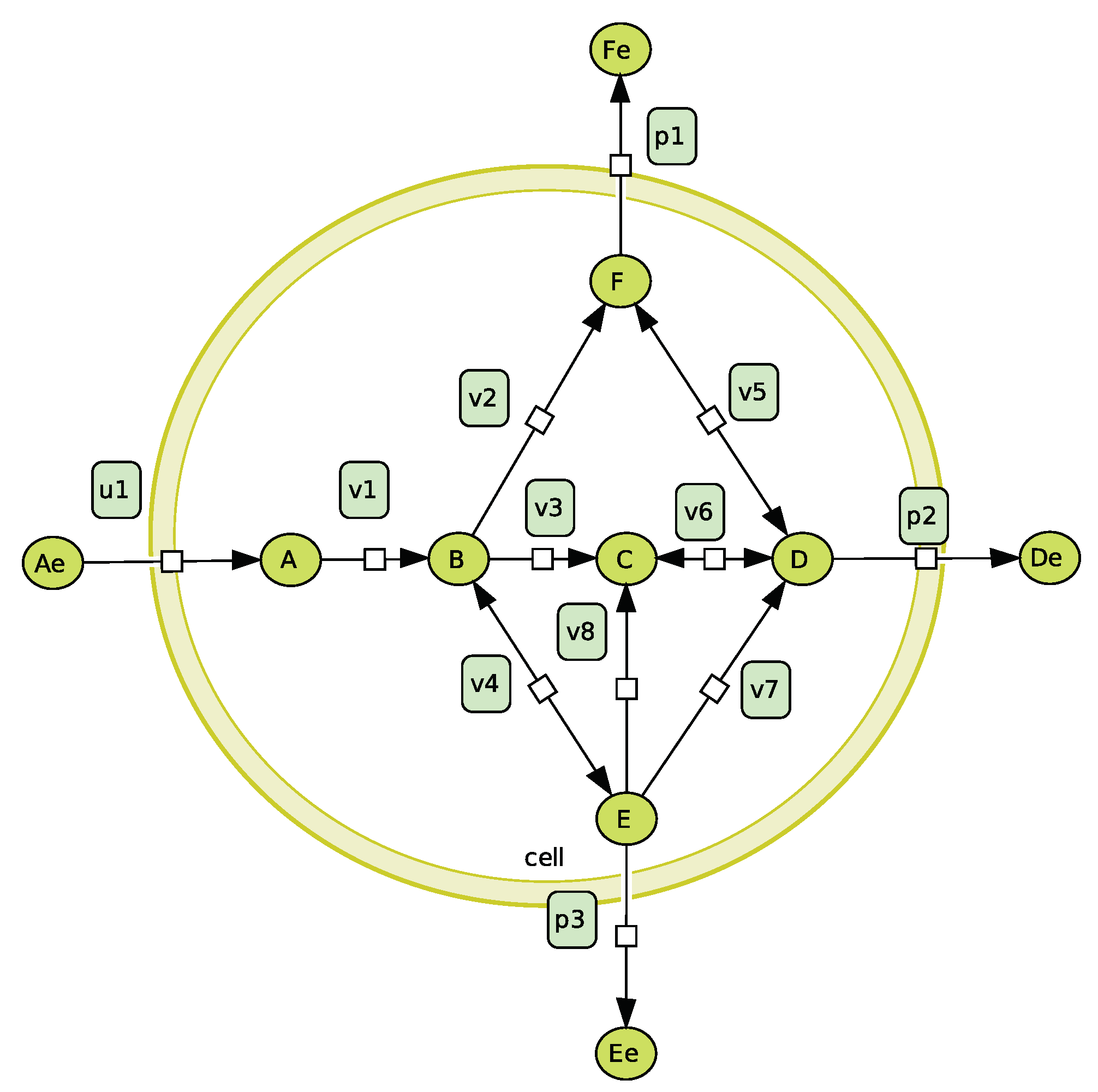
As we saw in the previous part, kinetic and constraint-based models are two interesting approaches to model metabolism. As they do not focus on the same aspects, they are rather complementary. On the one hand, a kinetic model is preferred to study detailed dynamical behaviours on a quantitative level while constraint-based approaches such as EFMs offer a global, genome scale view of the network and allow qualitative analysis. On the other hand, a kinetic model needs a lot of information (kinetic laws, parameters) while constraint-based approaches generally need less detailed information. In this part, we review the articles of Machado et al. [80] and of Schwartz and Kanehisa [81,82]. These papers effectively use the complementarity of constraint-based and kinetic models and show how both modeling approaches can be used in conjunction to obtain interesting results. We propose to illustrate their work on the simple network depicted in Figure 2. We thus build the following differential system:
where
To simplify, we assume that the extracellular concentration is constant and fixed to 5. The other parameters are:
| Name | |||||||||
| Value | 0.5 | 10 | 1 | 5 | 100 | 3.4 | 0.1 | 0.1 | 0.5 |
| Name | |||||||||
| Value | 7 | 0.1 | 4 | 10 | 1 | 10 | 0.1 |
We also build a constraint-based model from this network. This model is represented by:
where is the stoichiometric matrix of the network of Figure 2 which is also used in the differential system (9) and . In Figure 3, we present the elementary flux modes of . To compare the flux distributions obtained with the differential system and those obtained with the constraint-based model, we bound the fluxes of by the corresponding (100 or 200) of (10). By an abuse of language, we call this bounded cone . In Figure 4, we show a graphical representation of this cone by projecting it on different couples of reaction fluxes. This figure has been done by projecting the elementary flux vectors [26].
4.1. Using the Differential System to Reduce the Solution Space
We now present how we can use the differential system (9) to help analyse the cone . The following is inspired from [80] by Machado et al.
By simulating System (9), we observe that for a large range of parameters (and of initial conditions), the system seems to converge towards an equilibrium point denoted by . For an equilibrium state , since by definition . Thus, the kinetically feasible solution space of our example, as defined in [80] by
is a subset of . The reason behind this is the fact that and share the same stoichiometric matrix and the same set of irreversible reactions. It is still true when is bounded by the maximal values of the reaction rates of the system as in Figure 4.
In [80], Machado et al. numerically prove on their example (the model of central carbon metabolism of Escherichia coli from Chassagnole et al. [16]) that is equal to . In our example, we visually compared these two spaces. To visualise , we sample the parameter space by allowing each parameter to vary between and times their default value to mimic unbounded parameters and we run simulations to find the equilibria. By projecting each equilibrium flux, we obtain the same figure as in Figure 4, numerically showing that the pairwise projections of and overlap.
Therefore, by simulating the differential system with different parameter values and projecting the corresponding equilibria, we can directly visualise the impact of kinetic parameters on the cone . Let us assume for instance that the parameter only varies between 4 and 6 while the other parameters vary in a large range: between and times their default value. We then obtain Figure 5.
We can see on this figure how directly impact the values of and at steady-state. We are also able to see how the effects of this parameter propagate into the network and limit the range of the fluxes in the cone . In [80], Machado et al. also study how the reduction of the range of variation could reduce and by extension . In particular, they define a relative volume estimation to measure how much is reduced when the parameter range is reduced. They apply this on two versions of the model: the model with normal uptake of glucose and the model with maximal uptake of glucose. They find that they could halve by limiting the parameter variation between and times their initial values for the normal uptake of glucose model and between and for the maximal uptake ones.
Thus, the use of a differential system allows the direct integration of information into CBM we cannot integrate otherwise. In the next part, we present the opposite: how we can use the elementary flux modes to help the analysis of a differential system.
4.2. Using EFMs to Help Analyse the Differential System
Analysing a differential system is not an easy task. In particular, in the case of metabolism, it requires understanding the complex reaction network in order to be able to interpret the simulations of the system. As presented, elementary flux modes represent a useful tool to interpret metabolic network [84]. In particular, EFMs represent elementary metabolic functions and they provide a basis for the functional interpretation of a biochemical system [82]. Thus, in our example, since flux distributions at equilibrium lie in , we can use the elementary flux modes to decompose them and help the analysis of this system.
Inspired by [82], we numerically computed the equilibrium of System (9) for different values of and we decomposed into elementary flux modes the equilibrium fluxes. We present in Figure 6 (left) the evolution of this decomposition according to . On this figure, we can observe how the metabolic behaviour changes with and in particular the shifts in which pathway(s) the system uses. As expected, the use of EFM 4 and EFM 5, the two EFMs using , decreases when increases. We can also see on this figure how our system redirect the input flow on EFMs 6 and 8. On the right part of this figure, we regrouped the EFMs by the metabolite they produce (D, E and F). We can note on this figure that the production of E and F are highly affected by : the increase of this parameter leads to an increase in the production of E and a decrease in the production of F. It seems that when the system cannot use the pathway represented by EFM 4, it switches to the EFM 6. On this figure, we can also notice that the production of D is little affected by , EFM 8 compensating the decrease of use of EFM 5. Thus, decomposing flux distributions at equilibrium into EFMs helps us to understand how our system reacts to change in parameter(s) and more generally it helps us to understand its behaviours.
To obtain the decomposition of flux distribution into EFMs, we used a property of our differential system: when is negative and when we impose a conformal sum (a sum without cancellation), the solution of , where E is the matrix of EFMs, the flux distribution to be decomposed and the coefficient of the decomposition, is unique. To force to be negative, we change and to 300 and 0.001. In general however, the decomposition is not unique and we have to choose a criterion to select a solution. In [85], Poolman et al. use the Moore-Penrose generalized inverse of the matrix of EFMs to decompose a flux distribution. This method presents advantages: it is possible to decompose a partially known flux distribution and it can estimate the error of experimental measure. In [81,82], Schwartz and Kanehisa decompose a flux distribution by minimising the euclidean norm of the coefficient vector to promote EFMs that are close to the actual flux distribution. They apply this method to analyse the equilibrium flux of a differential system. They measure how parameter perturbations affect this system and identify a subset of parameters that have a important impact on the equilibrium. Nookaew et al., on the contrary, maximise the number of active EFMs in their decomposition, as the cells are likely to use as many pathways as possible to assure their robustness [83]. All of these methods need the computation of all the EFMs to be used and as explained before, it can be a limitation when the number of EFMs is too important. Chan and Ji in [86] decompose a flux distribution without the computation of all the EFMs based on the notion of non-decomposability of the EFMs. They define a recursive algorithm based on the question: is the current flux distribution decomposable? If the answer is no, then this flux distribution is an EFM and is part of the distribution flux we want to decompose. If the answer is yes, then we have to find such that and restart the algorithm with . This method allows us to decompose steady-state flux distribution of large network and ensure the conformity of the decomposition.
The power of EFMs to describe metabolic behaviours is also used in the analysis of fluxomics data. Principal Component Analysis (PCA) is a classical tool to analyse such data. However the principal components, one of the output of a PCA, are difficult to analyse from a biological point of view due to the absence of link with the structure of the metabolic network. Various authors suggest to combine PCA with EFMs by forcing the principal components to be EFMs [87,88,89]. Folch-Fortuny et al. [88] as well as Bhadra et al. [89] are even able to decompose flux distributions that are not in , which is not (yet) possible for one flux distribution at a time.
5. Conclusions
In this review, we presented the two main approaches to model metabolism dynamics: kinetic and constraint-based modelling (CBM). These two approaches represent the metabolism from two complementary points of view: kinetic models depict the evolution of metabolite concentrations in time in networks where detailed enzymatic mechanisms are known while constraint-based models focus on metabolic fluxes at steady-state of genome-scale networks.
Constraint-based models have been improved over the years to overcome certain limitations. First, time has been made explicit into FBA models in the framework dFBA. Then, this framework has also been extended by combining it with Boolean networks to incorporate genetic regulations. This extension allowed the modelling of some metabolic behaviours that were not recovered by dFBA alone. Another breakthrough has been made with the integration of enzymes cost, key element of metabolism, into the constraint-based modelling process. On the other hand, kinetic models have been improved to incorporate new features of metabolism. In particular, efforts have been made to include some aspects of metabolic enzymes (their regulations, their production, …) into ODE systems.
Finally both frameworks prove rather complementary to analyse the dynamical behaviours of a metabolic network. On an example, we showed two aspects of this complementarity. First simulating a kinetic model allows reducing the flux cone and observe the effects of certain parameters on the set of admissible fluxes. Second, qualitative features given by a CBM, such as EFM, prove a valuable tool to interpret asymptotic behaviours of an ODE model. The latter is limited to asymptotics, as only equilibrium fluxes are in the cone. Other decompositions, such as Elementary Growth Modes proposed by Müller [27], may be used to generalise this approach and go toward a decomposition of a whole trajectory.
Supplementary Materials
The following are available online at https://0-www-mdpi-com.brum.beds.ac.uk/article/10.3390/pr9101701/s1, Figure S1: Pairwise projection of the solution space used as an example in the article, Figure S2: Effects of parameter on .
Author Contributions
Conceptualization, C.M., S.P. and L.T.; writing—original draft, C.M. and S.P.; writing—review and editing, C.M., S.P. and L.T.; visualization, C.M. and L.T. All authors have read and agreed to the published version of the manuscript.
Funding
This research received no external funding.
Institutional Review Board Statement
Not applicable.
Informed Consent Statement
Not applicable.
Data Availability Statement
Not applicable.
Conflicts of Interest
The authors declare no conflict of interest.
Abbreviations
The following abbreviations are used in this manuscript:
| CBM | Constraint-Based Modelling |
| EFM | Elementary Flux Modes |
| FBA | Flux Balance Analysis |
| ODE | Ordinary Differential Equations |
| LP | Linear Programming |
References
- da Veiga Moreira, J.; Hamraz, M.; Abolhassani, M.; Schwartz, L.; Jolicoeur, M.; Peres, S. Metabolic Therapies Inhibit Tumor Growth in Vivo and in Silico. Sci. Rep. 2019, 9, 3153. [Google Scholar] [CrossRef] [PubMed] [Green Version]
- Robitaille, J.; Chen, J.; Jolicoeur, M. A Single Dynamic Metabolic Model Can Describe mAb Producing CHO Cell Batch and Fed-Batch Cultures on Different Culture Media. PLoS ONE 2015, 10, e0136815. [Google Scholar] [CrossRef] [PubMed]
- Ciesielski, A.; Grzywacz, R. Process Maps with Metabolic Constraints for Bioethanol Production by Continuous Fermentation. Chem. Eng. Sci. 2021, 229, 116134. [Google Scholar] [CrossRef]
- Park, H.; Patel, A.; Hunt, K.A.; Henson, M.A.; Carlson, R.P. Artificial Consortium Demonstrates Emergent Properties of Enhanced Cellulosic-Sugar Degradation and Biofuel Synthesis. NPJ Biofilms Microbiomes 2020, 6, 59. [Google Scholar] [CrossRef]
- Orth, J.D.; Conrad, T.M.; Na, J.; Lerman, J.A.; Nam, H.; Feist, A.M.; Palsson, B.O. A Comprehensive Genome-Scale Reconstruction of Escherichia Coli Metabolism–2011. Mol. Syst. Biol. 2014, 7, 535. [Google Scholar] [CrossRef]
- Brunk, E.; Sahoo, S.; Zielinski, D.C.; Altunkaya, A.; Dräger, A.; Mih, N.; Gatto, F.; Nilsson, A.; Preciat Gonzalez, G.A.; Aurich, M.K.; et al. Recon3D Enables a Three-Dimensional View of Gene Variation in Human Metabolism. Nat. Biotechnol. 2018, 36, 272–281. [Google Scholar] [CrossRef]
- da Veiga Moreira, J.; Peres, S.; Steyaert, J.M.; Bigan, E.; Paulevé, L.; Nogueira, M.L.; Schwartz, L. Cell Cycle Progression Is Regulated by Intertwined Redox Oscillators. Theor. Biol. Med. Model. 2015, 12, 10. [Google Scholar] [CrossRef] [Green Version]
- Moulin, C.; Tournier, L.; Peres, S. Using a Hybrid Approach to Model Central Carbon Metabolism Across the Cell Cycle. In Hybrid Systems Biology; Češka, M., Paoletti, N., Eds.; Springer International Publishing: Cham, Switzerland, 2019; Volume 11705, pp. 132–146. [Google Scholar] [CrossRef]
- Monod, J.; Wyman, J.; Changeux, J.P. On the Nature of Allosteric Transitions: A Plausible Model. J. Mol. Biol. 1965, 12, 88–118. [Google Scholar] [CrossRef]
- Gillespie, D.T. Exact Stochastic Simulation of Coupled Chemical Reactions. J. Phys. Chem. 1977, 81, 2340–2361. [Google Scholar] [CrossRef]
- Amar, P.; Bernot, G.; Norris, V. HSIM: A Simulation Programme to Study Large Assemblies of Proteins. J. Biol. Phys. Chem. 2004, 4, 79–84. [Google Scholar] [CrossRef] [Green Version]
- Klann, M.; Ganguly, A.; Koeppl, H. Hybrid Spatial Gillespie and Particle Tracking Simulation. Bioinformatics 2012, 28, i549–i555. [Google Scholar] [CrossRef] [Green Version]
- Baldan, P.; Cocco, N.; Marin, A.; Simeoni, M. Petri Nets for Modelling Metabolic Pathways: A Survey. Nat. Comput. 2010, 9, 955–989. [Google Scholar] [CrossRef] [Green Version]
- Ao, P. Metabolic Network Modelling: Including Stochastic Effects. Comput. Chem. Eng. 2005, 29, 2297–2303. [Google Scholar] [CrossRef] [Green Version]
- Bettenbrock, K.; Fischer, S.; Kremling, A.; Jahreis, K.; Sauter, T.; Gilles, E.D. A Quantitative Approach to Catabolite Repression in Escherichia coli. J. Biol. Chem. 2006, 281, 2578–2584. [Google Scholar] [CrossRef] [PubMed] [Green Version]
- Chassagnole, C.; Noisommit-Rizzi, N.; Schmid, J.W.; Mauch, K.; Reuss, M. Dynamic modeling of the central carbon metabolism ofEscherichia coli. Biotechnol. Bioeng. 2002, 79, 53–73. [Google Scholar] [CrossRef]
- Kim, O.D.; Rocha, M.; Maia, P. A Review of Dynamic Modeling Approaches and Their Application in Computational Strain Optimization for Metabolic Engineering. Front. Microbiol. 2018, 9, 1690. [Google Scholar] [CrossRef]
- Steuer, R.; Gross, T.; Selbig, J.; Blasius, B. Structural Kinetic Modeling of Metabolic Networks. Proc. Natl. Acad. Sci. USA 2006, 103, 11868–11873. [Google Scholar] [CrossRef] [Green Version]
- Grimbs, S.; Selbig, J.; Bulik, S.; Holzhütter, H.G.; Steuer, R. The Stability and Robustness of Metabolic States: Identifying Stabilizing Sites in Metabolic Networks. Mol. Syst. Biol. 2007, 3, 146. [Google Scholar] [CrossRef] [PubMed]
- Carbonaro, N.J.; Thorpe, I.F. Using Structural Kinetic Modeling To Identify Key Determinants of Stability in Reaction Networks. J. Phys. Chem. A 2017, 121, 4982–4992. [Google Scholar] [CrossRef] [PubMed]
- Girbig, D.; Grimbs, S.; Selbig, J. Systematic Analysis of Stability Patterns in Plant Primary Metabolism. PLoS ONE 2012, 7, e34686. [Google Scholar]
- Schuster, S.; Hilgetag, C. On Elementary Flux Modes in Biochemical Reaction Systems at Steady State. J. Biol. Syst. 1994, 2, 165–182. [Google Scholar] [CrossRef]
- Hunt, K.A.; Folsom, J.P.; Taffs, R.L.; Carlson, R.P. Complete Enumeration of Elementary Flux Modes through Scalable Demand-Based Subnetwork Definition. Bioinformatics 2014, 30, 1569–1578. [Google Scholar] [CrossRef]
- Acuña, V.; Chierichetti, F.; Lacroix, V.; Marchetti-Spaccamela, A.; Sagot, M.F.; Stougie, L. Modes and Cuts in Metabolic Networks: Complexity and Algorithms. Biosystems 2009, 95, 51–60. [Google Scholar] [CrossRef] [PubMed] [Green Version]
- Morterol, M.; Dague, P.; Peres, S.; Simon, L. Minimality of Metabolic Flux Modes under Boolean Regulation Constraints. In Proceedings of the 12th International Workshop on Constraint-Based Methods for Bioinformatics (WCB’16), Toulouse, France, 5 September 2016; pp. 65–81. [Google Scholar]
- Klamt, S.; Regensburger, G.; Gerstl, M.P.; Jungreuthmayer, C.; Schuster, S.; Mahadevan, R.; Zanghellini, J.; Müller, S. From Elementary Flux Modes to Elementary Flux Vectors: Metabolic Pathway Analysis with Arbitrary Linear Flux Constraints. PLoS Comput. Biol. 2017, 13, e1005409. [Google Scholar] [CrossRef] [PubMed]
- Müller, S. Elementary Growth Modes/Vectors and Minimal Autocatalytic Sets for Kinetic/Constraint-Based Models of Cellular Growth. bioRxiv 2021. [Google Scholar] [CrossRef]
- Varma, A.; Palsson, B. Metabolic Flux Balancing: Basic concepts, scientific and practical use. Nat. Biotechnol. 1994, 12, 994–998. [Google Scholar] [CrossRef]
- Mahadevan, R.; Schilling, C. The effects of alternate optimal solutions in constraint-based genome-scale metabolic models. Metab. Eng. 2003, 5, 264–276. [Google Scholar] [CrossRef]
- Feist, A.M.; Palsson, B.O. The Biomass Objective Function. Curr. Opin. Microbiol. 2010, 13, 344–349. [Google Scholar] [CrossRef] [Green Version]
- García Sánchez, C.E.; Torres Sáez, R.G. Comparison and Analysis of Objective Functions in Flux Balance Analysis. Biotechnol. Prog. 2014, 30, 985–991. [Google Scholar] [CrossRef]
- Montezano, D.; Meek, L.; Gupta, R.; Bermudez, L.E.; Bermudez, J.C.M. Flux Balance Analysis with Objective Function Defined by Proteomics Data—Metabolism of Mycobacterium Tuberculosis Exposed to Mefloquine. PLoS ONE 2015, 10, e0134014. [Google Scholar] [CrossRef]
- Peres, S.; Jolicoeur, M.; Moulin, C.; Dague, P.; Schuster, S. How Important Is Thermodynamics for Identifying Elementary Flux Modes? PLoS ONE 2017, 12, e0171440. [Google Scholar] [CrossRef] [PubMed]
- Segel, I.H. Enzyme Kinetics: Behavior and Analysis of Rapid Equilibrium and Steady State Enzyme Systems; Wiley: New York, NY, USA, 1993. [Google Scholar]
- Smallbone, K.; Mendes, P. Large-Scale Metabolic Models: From Reconstruction to Differential Equations. Ind. Biotechnol. 2013, 9, 179–184. [Google Scholar] [CrossRef] [Green Version]
- Khodayari, A.; Zomorrodi, A.R.; Liao, J.C.; Maranas, C.D. A kinetic model of Escherichia coli core metabolism satisfying multiple sets of mutant flux data. Metab. Eng. 2014, 25, 50–62. [Google Scholar] [CrossRef] [PubMed]
- Khodayari, A.; Maranas, C.D. A genome-scale Escherichia coli kinetic metabolic model k-ecoli457 satisfying flux data for multiple mutant strains. Nat. Commun. 2016, 7, 13806. [Google Scholar] [CrossRef] [PubMed]
- Varma, A.; Palsson, B.O. Stoichiometric Flux Balance Models Quantitatively Predict Growth and Metabolic By-Product Secretion in Wild-Type Escherichia Coli W3110. Appl. Environ. Microbiol. 1994, 60, 3724–3731. [Google Scholar] [CrossRef] [Green Version]
- Mahadevan, R.; Edwards, J.; Doyle, F. Dynamic Flux Balance Analysis of Diauxic Growth in Escherichia coli. Biophys. J. 2002, 83, 1331–1340. [Google Scholar] [CrossRef] [Green Version]
- Höffner, K.; Harwood, S.M.; Barton, P.I. A Reliable Simulator for Dynamic Flux Balance Analysis. Biotechnol. Bioeng. 2013, 110, 792–802. [Google Scholar] [CrossRef] [PubMed]
- Hjersted, J.L.; Henson, M.A. Optimization of Fed-Batch Saccharomyces Cerevisiae Fermentation Using Dynamic Flux Balance Models. Biotechnol. Prog. 2008, 22, 1239–1248. [Google Scholar] [CrossRef]
- da Veiga Moreira, J.; Jolicoeur, M.; Schwartz, L.; Peres, S. Fine-tuning mitochondrial activity in Yarrowia lipolytica for citrate overproduction. Sci. Rep. 2021, 11, 878. [Google Scholar] [CrossRef]
- Kuriya, Y.; Araki, M. Dynamic Flux Balance Analysis to Evaluate the Strain Production Performance on Shikimic Acid Production in Escherichia coli. Metabolites 2020, 10, 198. [Google Scholar] [CrossRef]
- Hanly, T.J.; Henson, M.A. Dynamic flux balance modeling of microbial co-cultures for efficient batch fermentation of glucose and xylose mixtures. Biotechnol. Bioeng. 2011, 108, 376–385. [Google Scholar] [CrossRef] [PubMed] [Green Version]
- Zhao, X.; Noack, S.; Wiechert, W.; von Lieres, E. Dynamic Flux Balance Analysis with Nonlinear Objective Function. J. Math. Biol. 2017, 75, 1487–1515. [Google Scholar] [CrossRef]
- Dromms, R.A.; Lee, J.Y.; Styczynski, M.P. LK-DFBA: A Linear Programming-Based Modeling Strategy for Capturing Dynamics and Metabolite-Dependent Regulation in Metabolism. BMC Bioinform. 2020, 21, 93. [Google Scholar] [CrossRef] [PubMed]
- Gomez, J.A.; Höffner, K.; Barton, P.I. DFBAlab: A fast and reliable MATLAB code for dynamic flux balance analysis. BMC Bioinform. 2014, 15, 409. [Google Scholar] [CrossRef] [PubMed] [Green Version]
- Scott, F.; Wilson, P.; Conejeros, R.; Vassiliadis, V.S. Simulation and Optimization of Dynamic Flux Balance Analysis Models Using an Interior Point Method Reformulation. Comput. Chem. Eng. 2018, 119, 152–170. [Google Scholar] [CrossRef] [Green Version]
- Bordbar, A.; Yurkovich, J.T.; Paglia, G.; Rolfsson, O.; Sigurjónsson, O.E.; Palsson, B.O. Elucidating dynamic metabolic physiology through network integration of quantitative time-course metabolomics. Sci. Rep. 2017, 7, 46249. [Google Scholar] [CrossRef] [Green Version]
- Covert, M.W.; Schilling, C.H.; Palsson, B. Regulation of Gene Expression in Flux Balance Models of Metabolism. J. Theor. Biol. 2001, 213, 73–88. [Google Scholar] [CrossRef] [Green Version]
- Covert, M.W.; Knight, E.M.; Reed, J.L.; Herrgard, M.J.; Palsson, B.Ø. Integrating High-Throughput and Computational Data Elucidates Bacterial Networks. Nature 2004, 429, 92–96. [Google Scholar] [CrossRef]
- Covert, M.W.; Xiao, N.; Chen, T.J.; Karr, J.R. Integrating Metabolic, Transcriptional Regulatory and Signal Transduction Models in Escherichia coli. Bioinformatics 2008, 24, 2044–2050. [Google Scholar] [CrossRef] [Green Version]
- Min Lee, J.; Gianchandani, E.P.; Eddy, J.A.; Papin, J.A. Dynamic Analysis of Integrated Signaling, Metabolic, and Regulatory Networks. PLoS Comput. Biol. 2008, 4, e1000086. [Google Scholar] [CrossRef] [Green Version]
- Thuillier, K.; Baroukh, C.; Bockmayr, A.; Cottret, L.; Paulevé, L.; Siegel, A. Learning Boolean Controls in Regulated Metabolic Networks: A Case-Study. In Proceedings of the 19th International Conference on Computational Methods in Systems Biology, Bordeaux, France, 22 September 2021. [Google Scholar]
- Peres, S.; Morterol, M.; Simon, L. SAT-Based Metabolics Pathways Analysis without Compilation. In Lecture Note in Bioinformatics; Mendes, J.D.P., Smallbone, K., Eds.; Springer International Publishing: Berlin, Germany, 2014; Volume 8859, pp. 20–31. [Google Scholar]
- Mahout, M.; Carlson, R.P.; Peres, S. Answer Set Programming for Computing Constraints-Based Elementary Flux Modes: Application to Escherichia coli Core Metabolism. Processes 2020, 8, 1649. [Google Scholar] [CrossRef]
- Janhunen, T.; Kaminski, R.; Ostrowski, M.; Schaub, T.; Schellhorn, S.; Wanko, P. Clingo Goes Linear Constraints over Reals and Integers. arXiv 2017, arXiv:1707.04053. [Google Scholar] [CrossRef] [Green Version]
- Goelzer, A.; Fromion, V.; Scorletti, G. Cell design in bacteria as a convex optimization problem. In Proceedings of the 48th IEEE Conference on Decision and Control, Shanghai, China, 15–18 December 2009; pp. 4517–4522. [Google Scholar]
- Goelzer, A.; Fromion, V.; Scorletti, G. Cell design in bacteria as a convex optimization problem. Automatica 2011, 47, 1210–1218. [Google Scholar] [CrossRef]
- Goelzer, A.; Muntel, J.; Chubukov, V.; Jules, M.; Prestel, E.; Nolker, R.; Mariadassou, M.; Aymerich, S.; Hecker, M.; Noirot, P.; et al. Quantitative prediction of genome-wide resource allocation in bacteria. Metab. Eng. 2015, 32, 232–243. [Google Scholar] [CrossRef] [PubMed]
- Bulović, A.; Fischer, S.; Dinh, M.; Golib, F.; Liebermeister, W.; Poirier, C.; Tournier, L.; Klipp, E.; Fromion, V.; Goelzer, A. Automated Generation of Bacterial Resource Allocation Models. Metab. Eng. 2019, 55, 12–22. [Google Scholar] [CrossRef] [PubMed] [Green Version]
- Tournier, L.; Goelzer, A.; Fromion, V. Optimal Resource Allocation Enables Mathematical Exploration of Microbial Metabolic Configurations. J. Math. Biol. 2017, 75, 1349–1380. [Google Scholar] [CrossRef] [PubMed]
- Jeanne, G.; Goelzer, A.; Tebbani, S.; Dumur, D.; Fromion, V. Dynamical resource allocation models for bioreactor optimization. IFAC-PapersOnLine 2018, 51, 20–23. [Google Scholar] [CrossRef]
- Jeanne, G.; Goelzer, A.; Tebbani, S.; Dumur, D.; Fromion, V. Towards a Realistic and Integrated Strain Design in Batch Bioreactor. In Proceedings of the 2018 IEEE Conference on Decision and Control (CDC), Miami, FL, USA, 17–19 December 2018; pp. 2698–2703. [Google Scholar] [CrossRef] [Green Version]
- Lerman, J.A.; Hyduke, D.R.; Latif, H.; Portnoy, V.A.; Lewis, N.E.; Orth, J.D.; Schrimpe-Rutledge, A.C.; Smith, R.D.; Adkins, J.N.; Zengler, K.; et al. In silico method for modelling metabolism and gene product expression at genome scale. Nat. Commun. 2012, 3, 929. [Google Scholar] [CrossRef] [Green Version]
- Liu, J.K.; O’Brien, E.J.; Lerman, J.A.; Zengler, K.; Palsson, B.O.; Feist, A.M. Reconstruction and Modeling Protein Translocation and Compartmentalization in Escherichia coli at the Genome-Scale. BMC Syst. Biol. 2014, 8, 110. [Google Scholar] [CrossRef] [Green Version]
- Lloyd, C.J.; Ebrahim, A.; Yang, L.; King, Z.A.; Catoiu, E.; O’Brien, E.J.; Liu, J.K.; Palsson, B.O. COBRAme: A Computational Framework for Genome-Scale Models of Metabolism and Gene Expression. PLoS Comput. Biol. 2018, 14, e1006302. [Google Scholar] [CrossRef]
- Yang, L.; Ebrahim, A.; Lloyd, C.J.; Saunders, M.A.; Palsson, B.O. DynamicME: Dynamic simulation and refinement of integrated models of metabolism and protein expression. BMC Syst. Biol. 2019, 13, 2. [Google Scholar] [CrossRef] [Green Version]
- Waldherr, S.; Oyarzun, D.A.; Bockmayr, A. Dynamic optimization of metabolic networks coupled with gene expression. J. Theor. Biol. 2015, 365, 469–485. [Google Scholar] [CrossRef] [Green Version]
- Ramkrishna, D. A Cybernetic Perspective of Microbial Growth. In Foundations of Biochemical Engineering; American Chemical Society: Washington, DC, USA, 1983; Chapter 7; pp. 161–178. [Google Scholar] [CrossRef]
- Young, J.D.; Henne, K.L.; Morgan, J.A.; Konopka, A.E.; Ramkrishna, D. Integrating cybernetic modeling with pathway analysis provides a dynamic, systems-level description of metabolic control. Biotechnol. Bioeng. 2008, 100, 18. [Google Scholar] [CrossRef]
- Kim, J.I.; Varner, J.D.; Ramkrishna, D. A hybrid model of anaerobic E. coli GJT001: Combination of elementary flux modes and cybernetic variables. Biotechnol. Prog. 2008, 24, 993–1006. [Google Scholar] [CrossRef]
- Song, H.S.; Ramkrishna, D. When is the Quasi-Steady-State Approximation Admissible in Metabolic Modeling? When Admissible, What Models are Desirable? Ind. Eng. Chem. Res. 2009, 48, 7976–7985. [Google Scholar] [CrossRef]
- Song, H.S.; Ramkrishna, D. Prediction of metabolic function from limited data: Lumped hybrid cybernetic modeling (L-HCM). Biotechnol. Bioeng. 2010, 106, 271–284. [Google Scholar] [CrossRef] [PubMed]
- Song, H.S.; Ramkrishna, D.; Pinchuk, G.E.; Beliaev, A.S.; Konopka, A.E.; Fredrickson, J.K. Dynamic modeling of aerobic growth of Shewanella oneidensis. Predicting triauxic growth, flux distributions, and energy requirement for growth. Metab. Eng. 2013, 15, 25–33. [Google Scholar] [CrossRef]
- Tourigny, D.S. Dynamic metabolic resource allocation based on the maximum entropy principle. J. Math. Biol. 2020, 80, 2395–2430. [Google Scholar] [CrossRef]
- Lunze, J.; Lamnabhi-Lagarrigue, F. (Eds.) Handbook of Hybrid Systems Control: Theory, Tools, Applications; Cambridge University Press: Cambridge, MA, USA, 2009. [Google Scholar] [CrossRef] [Green Version]
- Liu, L.; Bockmayr, A. Formalizing Metabolic-Regulatory Networks by Hybrid Automata. Acta Biotheor. 2020, 68, 73–85. [Google Scholar] [CrossRef] [PubMed]
- Liu, L.; Bockmayr, A. Regulatory Dynamic Enzyme-Cost Flux Balance Analysis: A Unifying Framework for Constraint-Based Modeling. J. Theor. Biol. 2020, 501, 110317. [Google Scholar] [CrossRef] [PubMed]
- Machado, D.; Costa, R.S.; Ferreira, E.C.; Rocha, I.; Tidor, B. Exploring the Gap between Dynamic and Constraint-Based Models of Metabolism. Metab. Eng. 2012, 14, 112–119. [Google Scholar] [CrossRef] [PubMed]
- Schwartz, J.M.; Kanehisa, M. A Quadratic Programming Approach for Decomposing Steady-State Metabolic Flux Distributions onto Elementary Modes. Bioinformatics 2005, 21, ii204–ii205. [Google Scholar] [CrossRef] [PubMed]
- Schwartz, J.M.; Kanehisa, M. Quantitative Elementary Mode Analysis of Metabolic Pathways: The Example of Yeast Glycolysis. BMC Bioinform. 2006, 7, 186. [Google Scholar] [CrossRef]
- Nookaew, I.; Meechai, A.; Thammarongtham, C.; Laoteng, K.; Ruanglek, V.; Cheevadhanarak, S.; Nielsen, J.; Bhumiratana, S. Identification of Flux Regulation Coefficients from Elementary Flux Modes: A Systems Biology Tool for Analysis of Metabolic Networks. Biotechnol. Bioeng. 2007, 97, 1535–1549. [Google Scholar] [CrossRef]
- Trinh, C.T.; Wlaschin, A.; Srienc, F. Elementary Mode Analysis: A Useful Metabolic Pathway Analysis Tool for Characterizing Cellular Metabolism. Appl. Microbiol. Biotechnol. 2009, 81, 813–826. [Google Scholar] [CrossRef] [PubMed] [Green Version]
- Poolman, M.G.; Venkatesh, K.V.; Pidcock, M.K.; Fell, D.A. A Method for the Determination of Flux in Elementary Modes, and Its Application to Lactobacillus Rhamnosus. Biotechnol. Bioeng. 2004, 88, 13. [Google Scholar] [CrossRef] [PubMed]
- Chan, S.H.J.; Ji, P. Decomposing Flux Distributions into Elementary Flux Modes in Genome-Scale Metabolic Networks. Bioinformatics 2011, 27, 2256–2262. [Google Scholar] [CrossRef] [PubMed] [Green Version]
- Folch-Fortuny, A.; Marques, R.; Isidro, I.A.; Oliveira, R.; Ferrer, A. Principal Elementary Mode Analysis (PEMA). Mol. Biosyst. 2016, 12, 737–746. [Google Scholar] [CrossRef] [PubMed] [Green Version]
- Folch-Fortuny, A.; Teusink, B.; Hoefsloot, H.C.; Smilde, A.K.; Ferrer, A. Dynamic Elementary Mode Modelling of Non-Steady State Flux Data. BMC Syst. Biol. 2018, 12, 71. [Google Scholar] [CrossRef] [PubMed]
- Bhadra, S.; Blomberg, P.; Castillo, S.; Rousu, J. Principal Metabolic Flux Mode Analysis. Bioinformatics 2018, 34, 2409–2417. [Google Scholar] [CrossRef] [PubMed] [Green Version]
Figure 1.
Graphical representation of the different frameworks evoked in this paper and their links. Each framework is categorised depending on its type: constraint-based or kinetic, and depending on some dynamical features it provides: explicit time, regulations or enzyme cost. An arrow from framework A to framework B indicates that B is an extension of A.

Figure 2.
Example of a production system. Inspired by [83].
Figure 2.
Example of a production system. Inspired by [83].

Figure 3.
Graphical representation of the nine elementary flux modes of defined by Equation (11). The bold lines represent the reactions that are active in each EFM. This figure was automatically drawn with EFMdraw [33].

Figure 4.
Pairwise projection of the solution space defined by Equation (11). Only the 6 first reactions are presented. The full picture is in Supplement Figure S1. On each plane, the black lines are the limits of the projection of the solution space while the grey area represents its interior. To obtain these figures, we project the Elementary Flux Vectors (EFV) on each plane. Each projection of EFV is seen as a point on the plane. As all EFV in our model are bounded, we determine the projection of the solution space by finding the bigger polygon (in the sense of inclusion) we can make from each point.

Figure 5.
Effects of parameter on . Pairwise projection of on the solution space when varies between 4 and 6 and when the other parameters vary between and time their default value. Only the 6 first reactions are presented. The full picture is in Supplement Figure S2.
Figure 5.
Effects of parameter on . Pairwise projection of on the solution space when varies between 4 and 6 and when the other parameters vary between and time their default value. Only the 6 first reactions are presented. The full picture is in Supplement Figure S2.

Figure 6.
Effects of parameter on the decomposition into elementary flux modes (EFMs) of flux distributions of system (9) at equilibrium. Left: Proportion of each EFM. Right: The EFMs are grouped according to the metabolite they produce.
Figure 6.
Effects of parameter on the decomposition into elementary flux modes (EFMs) of flux distributions of system (9) at equilibrium. Left: Proportion of each EFM. Right: The EFMs are grouped according to the metabolite they produce.

Publisher’s Note: MDPI stays neutral with regard to jurisdictional claims in published maps and institutional affiliations. |
© 2021 by the authors. Licensee MDPI, Basel, Switzerland. This article is an open access article distributed under the terms and conditions of the Creative Commons Attribution (CC BY) license (https://creativecommons.org/licenses/by/4.0/).
Share and Cite
MDPI and ACS Style
Moulin, C.; Tournier, L.; Peres, S. Combining Kinetic and Constraint-Based Modelling to Better Understand Metabolism Dynamics. Processes 2021, 9, 1701. https://0-doi-org.brum.beds.ac.uk/10.3390/pr9101701
AMA Style
Moulin C, Tournier L, Peres S. Combining Kinetic and Constraint-Based Modelling to Better Understand Metabolism Dynamics. Processes. 2021; 9(10):1701. https://0-doi-org.brum.beds.ac.uk/10.3390/pr9101701
Chicago/Turabian StyleMoulin, Cecile, Laurent Tournier, and Sabine Peres. 2021. "Combining Kinetic and Constraint-Based Modelling to Better Understand Metabolism Dynamics" Processes 9, no. 10: 1701. https://0-doi-org.brum.beds.ac.uk/10.3390/pr9101701
Note that from the first issue of 2016, this journal uses article numbers instead of page numbers. See further details here.