Experimental Evaluation of Axial Reaction Turbine Stage Bucket Losses ^†

Abstract

The article describes the measurement methods and data evaluation from a single-stage axial turbine with high reaction (50%). Four operating modes of the turbine were selected, in which the wake traversing behind nozzle and bucket with five-hole pneumatic probes took place. The article further focuses on the evaluation of bucket losses for all four measured operating modes, including the analysis of measurement uncertainties.

1. Introduction

The methodology and rules for calculating a turbine blading efficiency in the turbine stages design is one of the most valuable and secret know-how of steam/gas turbine manufacturers. The acquisition of new data for efficiency prediction and research aimed at increasing efficiency is important and is the long-term development goal of all turbine manufacturers. Spatial blade shaping in general is one of the main means of increasing the blading efficiency. It focuses primarily on reducing the effect of secondary flow and associated losses, but also on the targeted redistribution of certain flow parameters, not only along the blades lengths, but also within the stage, or indeed within the whole turbine flow path [1].

At Doosan Skoda Power (DSPW), an industrial partner of the Department of Power System Engineering, intensive development of new blading types has been carried out in the recent past. The development has focused mainly on nozzle shaping. Variants with simple and compound circumferential lean and flow controlled blades have been investigated. The work focused on the nozzle shaping while maintaining the original, prismatic, bucket blades. Some of the results have been presented, e.g., in [2,3,4,5].

In the following period, DSPW, traditional impulse conception turbines manufacturers, developed 3D blading with a slightly increased root reaction. This blading already included the shaping of both the nozzle and bucket blades. The aim of the shaping is primarily to reduce secondary losses in the blade channels. The three variants of the stage with different nozzle blade numbers were tested in turn. The results have been published, e.g., in [6,7,8,9,10,11,12,13,14,15]. This development resulted in an efficiency increase of about 2% in the high-pressure (HP) turbine section and 1.5% in the intermediate-pressure (IP) turbine section compared to the conventional prismatic blading. The proposed principles have also been successfully deployed in the practise many times [1].

In essence, the increased root reaction stages represent an evolutionary transition between the impulse and reaction turbine stage concepts. The current developments in 3D blading fields thus logically lead the DSPW towards reaction stage concepts.

The paper therefore describes part of the experimental results obtained in connection with the ongoing testing of high reaction turbine stages. Specifically, it deals with the measurement and evaluation of bucket losses at different operation modes of the turbine stage.

2. Test Rig Description

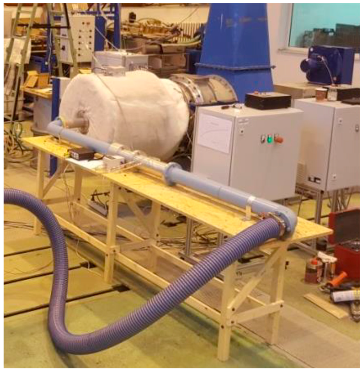
The experimental turbine test rig (VT-400) (see Figure 1) is a 1:2 scale model of an HP steam turbine part. The working medium is air sucked from the atmosphere by a compressor. The turbine stage is situated at the compressor suction. The compressor can achieve maximum a pressure drop of 12.5 kPa. The dynamometer measures RPM and torque. The mass flow of the working medium is determined by a standardized nozzle. Static pressure taps are located in individual sections of the turbine, and two 5-hole pneumatic probes are used for detailed flow field measurements [1,11].

At present, the three turbine stages with different reactions, which were designed by industrial partner Doosan Skoda Power, can be investigated. Their basic geometric parameters are listed in the following table (see

Table 1. Geometrical parameters of tested stages.

Nozzle			Bucket
Root diameter (mm)	DPNZL	400	Root diameter (mm)	DPBCK	400
Blade length (mm)	LNZL	45.5	Blade length (mm)	LBCK	47
Chord (mm)	cNZL	22.5	Output relative velocity angles (°)
Output absolute angle	α1	14.5°	Low reaction—LR (~25%)	β2LR	19.9°
			Mid reaction—MR (~35%)	β2MR	19.0°
			High reaction—HR (~50%)	β2HR	14.5°

). The currently measured stage is marked in red.) [1,11].

3. Measurement and Data Evaluation

Two basic measuring tasks can be performed on the turbine test rig. The aim of the first type is to determine the basic turbine stage characteristic, i.e., the dependence of the circumferential efficiency on the speed ratio $u_s/c_{02,iz}$ (ratio of circumferential velocity at mid blade radius and fictive (isentropic) velocity. In our case, the modes $\left(u_s/c_{02,iz}\right)$ are set by regulating a compressor (RPM), while a pressure drop on the turbine changes. From the measurement point of view, only static pressures in individual sections of the flow path (see Figure 2), input/output static pressures of the mass nozzle, data from the dynamometer (RPM and torque), stage output temperature and the mass nozzle output temperature are measured.

The second type of measurement is used for detailed flow fields measurement in the wake behind the nozzle and bucket. From these data it is possible to evaluate the radial distribution of losses, reaction, flow angles, Mach and Reynolds numbers. In this case, a constant mode is set at the beginning of the measurement $\left(u_s/c_{02,iz}=const.\right)$.The paper deals with the second type of measurement [11].

3.1. Probe Calibration

Wake traversing downstream of the nozzle and bucket is carried out using two five-hole pneumatic probes (serial no.: 15136-2). Both probes must be calibrated before operation. Calibration took place by air tunnel in the department laboratory (see Figure 3).

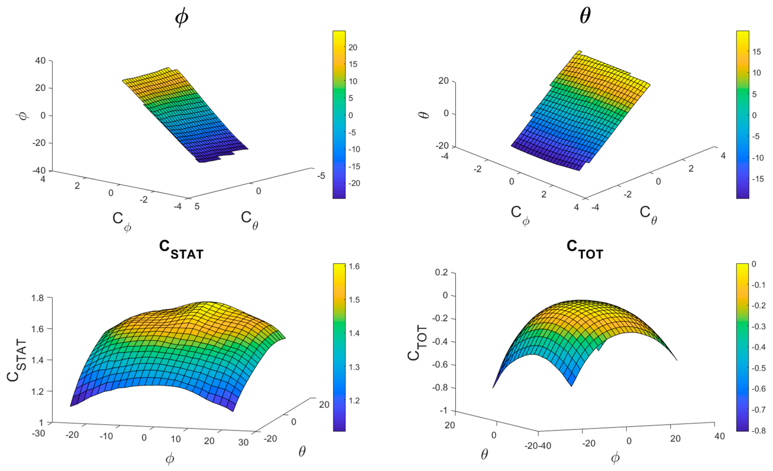
The calibration was realized by setting a certain angle θ, at which the pressures are measured for different values of the angle φ in the range φ = (−20°; 20°). Subsequently, the turning device is shifted by an angle θ and the pressures are measured again for the entire range of angles φ. The range of angles θ was also θ = (−20°; 20°). A Prandtl probe serves as a “standard” for determining static and total pressure. Calibration coefficients (two pressure, two angular) were calculated from obtained data [11].

$$\begin{array}{c}{C}_{STAT}=\frac{p_1-p_s}{p_1-p_m} ; C_{TOT}=\frac{p_1-p_c}{p_1-p_m}\\ C_{\phi }=\frac{p_2-p_3}{p_1-p_m} ; C_{\theta }=\frac{p_4-p_5}{p_1-p_m}\end{array}$$

The calibration pressure coefficients with the probe rotation angles together create data for 3D graphs. Mathematical interpretation of these 3D surfaces (see Figure 4) in the form of a regression equation root matrix is one of the main inputs in the evaluation process from the wake traversing behind the nozzle and bucket [11].

3.2. Data Evaluation Software

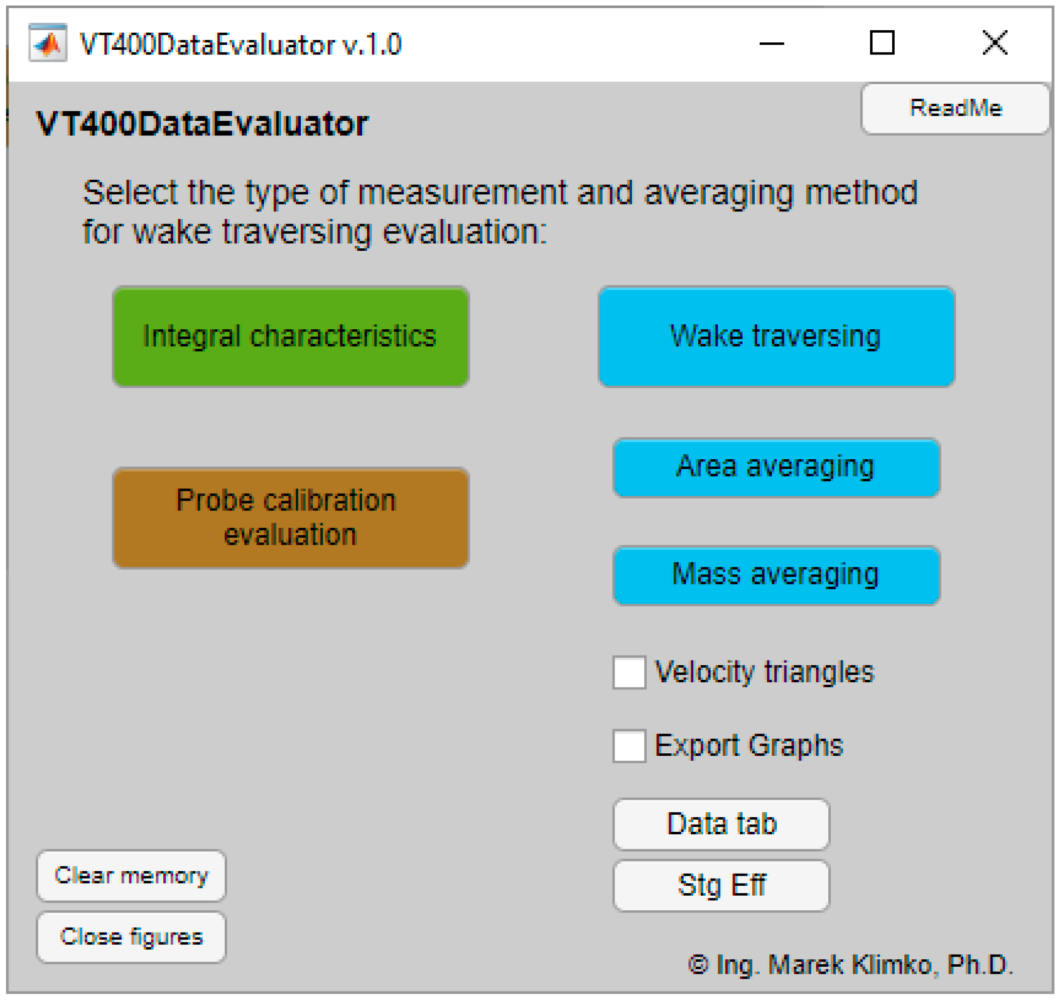
SW developed at the Department of Power System Engineering is used to evaluate data from the turbine. The SW was programmed in the “Matlab^®–App Designer” interface.

The home screen (Figure 5) offers several evaluation options. The green click button (“Integral characteristics”) evaluates the data from the first measurement type. This is therefore the basic turbine stage characteristic ${\eta }_{ST}=f\left(u_s/c_{02,iz}\right)$. The brown click button (“Probe calibration evaluation”) calculates the roots of the regression equations from the five-hole probes calibration surfaces.

A group of the blue click buttons allows to evaluate the second measurement type, i.e., in the case of wake traversing behind the nozzle and bucket. In the first step, when the “Wake traversing” option is selected, the program gradually prompts the user to select measured data, design blade angles, regression equation roots matrix and finally to select the number of measured radial planes. Subsequently, all necessary calculations will be performed. The next step is to choose the data reduction method. The program enables area averaging or averaging weighted by mass flow (in the case of incompressible flow by axial velocity only).

$$\begin{array}{c}\overline{\theta }=\frac{1}{S}{\displaystyle \int }\theta dS \to \frac{1}{S}{\displaystyle {\displaystyle \sum }_{i=1}^n}{\theta }_i·S_i\\ \overline{\theta }=\frac{\int \theta ·\rho ·\left|\overrightarrow{w}d\overrightarrow{S}\right|}{\int \rho ·\left|\overrightarrow{w}d\overrightarrow{S}\right|} \to \frac{{\sum }_{i=1}^n{\theta }_i·{\rho }_i·\left|{\overrightarrow{w}}_i·{\overrightarrow{S}}_i\right|}{{\sum }_{i=1}^n{\rho }_i·\left|{\overrightarrow{w}}_i·{\overrightarrow{S}}_i\right|}\end{array}$$

In the evaluation process, only the axial velocity is averaged over the area. Other parameters are averaged by mass flow over a multiple of the blade pitch. The area averaging method has a great weakness in the wake areas, where, for example, losses increase disproportionately. In mass flow averaging, the flow through these areas will be taken into account and the obtained values are therefore much closer to reality.

3.3. Mass Flow Evaluation

A mass flow is one of the main parameters for determining the useful turbine stage enthalpy gradients. The mass flow calculation through the measuring nozzle was performed according to the ČSN EN ISO 5167-3 standard. The initial relation is the following equation, in which, in addition to the geometric parameters and the difference in static pressure at the inlet and outlet of the nozzle, two coefficients also occur. The first one is the flow coefficient $c_q$, which is a function of the Reynolds number. Its course is shown in the figure (Figure 6).

$$\dot{m}=\frac{c_q}{\sqrt{1-{\beta }^4}}\epsilon \frac{\pi d^2}{4}\sqrt{2∆p_{cl}\rho } ; \beta =\frac{d}{D}$$

The second coefficient is the expansion factor ε determining the effect of the working medium compressibility. In addition to the ratio of nozzle diameters $\left(\beta \right)$, it is also a function of the inlet and outlet pressure $\left(\tau \right)$ ratio.

$$\epsilon =\sqrt{\left(\frac{\kappa {\tau }^{\frac{2}{\kappa }}}{\kappa -1}\right)\left(\frac{1-{\beta }^4}{1-{\beta }^4{\tau }^{\frac{2}{\kappa }}}\right)\left(\frac{1-{\tau }^{\frac{\kappa -1}{\kappa }}}{1-\tau }\right)} ; \tau =\frac{p_{cl2}}{p_{cl1}}$$

A calculated mass air flow represents the flow through the measuring loop. However, in order to evaluate the turbine stage efficiency, it is necessary to consider that this calculated value corresponds to the flow only through the nozzle, not the bucket. This is because the part of main flow flows through the bucket tip seal which does not generate useful stage work. Therefore, it is necessary to make a correction and subtract the tip leakage flow from the calculated mass flow.

$$\begin{array}{c}{\dot{m}}_{NZL}=\dot{m}\\ {\dot{m}}_{BCK}=\dot{m}-{\dot{m}}_L\end{array}$$

For bucket mass flow correction purposes, the tip leakage flow was calibrated. The design of the experimental turbine was modified so that it was possible to study the blowing and suction effects in the axial gap at the root blade section. This modification made it possible to carry out the tip leakage calibration (Figure 7).

In order to be able to determine the flow through the bucket tip seal only, it was necessary to cover the nozzle and bucket blading. To determine a tip leakage mass flow, a Venturi nozzle was placed in the inlet pipe (see Figure 8).

The calibration results were then compared with the labyrinth seal loss model correlations according to the authors Zalf [16] and Samoylovich [17].

$$\begin{array}{c}{\dot{m}}^Z=1.5S\sqrt{\frac{p_{V,in}}{v_{in}}}\sqrt{\kappa {\left(\frac{2}{\kappa +1}\right)}^{\frac{\kappa +1}{\kappa -1}}}\sqrt{\frac{1-{\left(\frac{p_{V,out}}{p_{V,in}}\right)}^2}{z-\ln \left(\frac{p_{V,out}}{p_{V,in}}\right)}}\\ {\dot{m}}^S=k\mu S\sqrt{\frac{p_{V,in}}{v_{in}}}\sqrt{\kappa {\left(\frac{2}{\kappa +1}\right)}^{\frac{\kappa +1}{\kappa -1}}}\sqrt{\frac{1-{\left(\frac{p_{V,out}}{p_{V,in}}\right)}^2}{z\left[1-{\left(\frac{p_{V,out}}{p_{V,in}}\right)}_{cr}\right]}-\frac{{\left(\frac{p_{V,out}}{p_{V,in}}\right)}_{cr}1-{\left(\frac{p_{V,out}}{p_{V,in}}\right)}^2}{z^2{\left[1-{\left(\frac{p_{V.out}}{p_{V,in}}\right)}_{cr}\right]}^2}}\end{array}$$

The following graph shows a comparison of the experiment with the analytical models (Figure 9). The results from the experiment showed good agreement with the analytical model according to Samoylovich. The Zalf correlation model deviates from the measured values with an increasing pressure drop on the seal, because this model does not fully include the labyrinth seal geometric parameters.

4. Results

The four operating turbine stage modes were selected for turbine speed 3000 RPM. One mode close to optimal operation $\left(u_s/c_{02,iz}~0.7\right)$ and three off-design modes. The velocity triangles of all measured modes are shown in Figure 10.

Bucket losses were evaluated based on the entropy increase definition. The radial distributions of the averaged bucket losses are shown in Figure 11.

$${\zeta }_{BCK}^{\left(s\right)}\cong \frac{T_2 · \left[-R · \ln \left(\frac{p_{2w}}{p_{1w}}\right)\right]}{\frac{w_2^2}{2}}$$

Figure 11 shows the area of the bucket blade mean radius, where the bucket losses dependence on the incidence is plotted.

The bucket inlet relative velocity angle radial distribution is shown in Figure 12.

The stated dependences represented mass-averaged data, i.e., one representative mean value of the monitored parameter was always determined for the selected blade radius. However, detailed wake traversing allows a visualization of the entire flow flied. For this purpose, a data post-processing software was created, the outputs of which are clear from the following figures (Figure 13).

It can be seen from the above figures (Figure 13) that the wake traversing was realized circumferentially over two blade pitches. At the root blade section, the working medium interaction with the rotor wheel end wall is significantly applied. At the blade tip area, it is possible to observe a local increase in losses due to the mixing of the labyrinth seal parasitic flow with main flow.

Estimation of Bucket Loss Coefficient Measurement Uncertainty

The bucket loss coefficient uncertainty measurement estimation was performed on a basis of methodology for determining the standard uncertainty for indirect measurements. In this methodology, the sought output quantity is a known function of input quantities that can be measured directly. The output estimate is determined as

$$y=f\left(x_1,x_2,\dots ,x_m\right)$$

The input quantities estimate is determined as follows:

$$u^2\left(y\right)={\displaystyle \sum }_{i=1}^m{A}_i^2{u}^2\left(x_i\right)$$

where $A_i$ represents the relevant sensitivity coefficient defined by:

$$A_i={\frac{\partial \left(X_1,X_2,\dots ,X_m\right)}{\partial X_i}|}_{X_1=x_1,\dots ,X_m=x_m}$$

In this case, the output variable is the evaluated bucket loss coefficient, which is a function of the measured parameters. An initial equation for the bucket loss evaluation from the entropy increase definition has been modified to include all measured parameters, which are determined by the appropriate sensitivity coefficients.

$${\zeta }_{BCK}^{\left(s\right)}=-\frac{R_v\ln \left\{\frac{\frac{{\sigma }_2}{2c_p}+{\sigma }_9{\sigma }_8}{\left(p_{1s}+p_b\right){\left[\frac{\frac{{\left({\sigma }_6-\cos \left({\alpha }_{1f}\right)\cos \left({\vartheta }_{1f}\right)\sqrt{2c_p{\sigma }_5}\right)}^2+2c_p\sin {\left({\alpha }_{1f}\right)}^2\cos {\left({\vartheta }_{1f}\right)}^2{\sigma }_5}{2c_p}+{\sigma }_9{\sigma }_8}{{\sigma }_9{\sigma }_8}\right]}^{\frac{\kappa }{\kappa -1}}}\right\}\left(\frac{{\sigma }_2}{c_p}-\frac{{\sigma }_1}{c_p}+2{\sigma }_9{\sigma }_8\right)}{{\sigma }_1}$$

where:

$$\begin{array}{l}{\sigma }_1={\left[{\sigma }_6+cos\left(\frac{\pi {\alpha }_{2f}}{180}\right){\sigma }_4\sqrt{2c_p{\sigma }_3}\right]}^2+2c_{p}sin{\left(\frac{\pi {\alpha }_{2f}}{180}\right)}^2{\sigma }_4{}^2{\sigma }_3\\ {\sigma }_2={\left[{\sigma }_6-cos\left(\frac{\pi {\alpha }_{1f}}{180}\right){\sigma }_7\sqrt{2c_p{\sigma }_5}\right]}^2+2c_{p}sin{\left(\frac{\pi {\alpha }_{1f}}{180}\right)}^2{\sigma }_7{}^2{\sigma }_5\\ {\sigma }_3={\sigma }_9{\left(\frac{p_{2c}+p_b}{p_{1s}+p_b}\right)}^{\frac{\kappa -1}{\kappa }}{\sigma }_8-{\sigma }_9{\left(\frac{p_{2s}+p_b}{p_{1s}+p_b}\right)}^{\frac{\kappa -1}{\kappa }}{\sigma }_8\\ {\sigma }_4=cos\left(\frac{\pi {\vartheta }_{2f}}{180}\right)\\ {\sigma }_5=t_{0s}-{\sigma }_9{\sigma }_8+\frac{S_{BCK}{\dot{m}}_{BCK}{\left(p_{0s}+p_b\right)}^2}{{\sigma }_{10}}\\ {\sigma }_6=\frac{\pi rn}{30}\\ {\sigma }_7=cos\left(\frac{\pi {\vartheta }_{1f}}{180}\right)\\ {\sigma }_8=t_{0s}+\frac{S_{BCK}^2{\dot{m}}_{BCK}^2{\left(p_{0s}+p_b\right)}^2}{{\sigma }_{10}}\\ {\sigma }_9={\left(\frac{p_{1s}+p_b}{p_{1c}+p_b}\right)}^{\frac{\kappa -1}{\kappa }}\\ {\sigma }_{10}=2R_v^2{c}_p{t}_{0s}^2\end{array}$$

At first, an estimate of the bucket loss coefficient uncertainty on the mean blade radius for the stage operating mode closest to the design conditions $\left(u_s/c_{02,iz}~0.7\right)$ was performed. Subsequently, an uncertainty estimate was performed for stage operating mode $\left(u_s/c_{02,iz}~0.83\right)$. The partial uncertainty diagrams describe Figure 14 and Figure 15.

The largest contribution to the total uncertainty is the uncertainty of measuring the angle ${\alpha }_{2f}$ (bucket probe rotation around its own axis). Influence of ${\alpha }_{1f}$ angle measurement is more pronounced in the optimally loaded stage mode. On the contrary, in the off-design mode, the uncertainty influence of the total and static pressure measurement behind the bucket begins to manifest itself more. Compared to the optimal stage load, the increase of the total measurement uncertainty is approximately 56% with analysed off-design load.

Due to the relatively high sensitivity of the ${\alpha }_{2f}$ (or even ${\alpha }_{1f}$) angle measurements, attention was paid to the installation and setup of both probes in the traversing device. Before starting the measurements, both probes were set to a neutral reference position from the geometric and aerodynamic points of view. Geometric adjustment of the initial positions of the probes was performed using a special protractor made using 3D printing (see Figure 16-left). The aerodynamic “zero” of the probes was experimentally determined using a wind tunnel (see Figure 16-right).

5. Conclusions

Bucket loss evaluation is a challenging task. The sensitivity analysis shows a significant effect of uncertainty in the bucket inlet and outlet flow angle measurements. In the more significant off-design modes, the uncertainty of total and static pressure measurement is also beginning to show. In addition, the bucket losses are strongly dependent on the bucket input flow parameters, which are difficult to determine by standard measurements with pneumatic probes. The current experimental device configuration allows to measure only one radial plane behind nozzle and one radial plane behind the bucket. However, the flow parameters in the axial gap between nozzle and bucket change. The actual flow parameters at the bucket input will therefore be different from the measured data.

More detailed information about the flow field near the bucket leading edges could be provided by the planned measurement using the PIV (Particle Image Velocimetry) visualization method, which will be supported by numerical simulation.

References

- Klimko, M.; Okresa, D. Measurements on the VT 400 Air Turbine. Acta Polytech. 2016, 56, 118–125. [Google Scholar] [CrossRef] [Green Version]
- Vomela, J. Experimental and numerical development of turbine blades of high efficiency. In Proceedings of the 5th European conference on Turbomachinery, Prague, Czech Republic, 17–22 March 2003; pp. 699–708. [Google Scholar]
- Vomela, J.; Milcak, P. The Development of High-Efficiency Turbine Blades; Cieplne Maszyny Przeplywowe; Turbomachinery; Technical University of Lodz: Lodz, Poland, 2005; pp. 557–564. [Google Scholar]
- Haller, B. Full 3D Turbine Blade Design; Lecture series “Secondary and Tip Clearance Flow in Axial Turbines”; Von Karman Institute of Fluid Dynamics: Sint-Genesius-Rode, Belgium, 1997. [Google Scholar]
- Sieverding, C.H. Recent Progress in the Understanding of Basic Aspects of Secondary Flows in Turbine Blade Passages. J. Eng. Gas Turbines Power 1985, 107, 248–257. [Google Scholar] [CrossRef]
- Milcak, P.; Sobczak, K. Experimental and Numerical Investigations of a Flow in the Stage with Compound Lean and Compound Twist Stator Blades; Power System Engineering, Thermodynamics & Flow ES 2017; University of West Bohemia: Pilsen, Czechia, 2007; pp. 153–160. [Google Scholar]
- Harrison, S. The Influence of Blade Lean on Turbine Losses. J. Turbomach. 1992, 114, 184–190. [Google Scholar] [CrossRef]
- Milcak, P.; Hoznedl, M. Measurement of flow fields on a turbine stage with 3D blades. In Experimental Fluid Mechanics; Technical University of Liberec: Liberec, Czechia, 2010; pp. 417–422. [Google Scholar]
- Milčák, P.; Hoznedl, M.; Zitek, P. Measurement on stages with 3D bladings and different relative width of stator blades. EPJ Web Conf. 2012, 25, 01054. [Google Scholar] [CrossRef] [Green Version]
- Milcak, P.; Zitek, P.; Hoznedl, M. Comparison of results from experimental testing of three variants of turbine stages with modern 3D blades. EPJ Web Conf. 2013, 45, 01063. [Google Scholar] [CrossRef] [Green Version]
- Klimko, M.; Žitek, P.; Lenhard, R. Measurement on Axial Reaction Turbine Stage. MATEC Web Conf. 2020, 328. [Google Scholar] [CrossRef]
- Uher, J.; Milcak, P.; Skach, R.; Fenderl, D.; Zitek, P.; Klimko, M. Experimental and Numerical Evaluation of Losses From Turbine Hub Clearance Flow. In Turbo Expo: Power for Land, Sea, and Air; American Society of Mechanical Engineers: New York, NY, USA, 2019. [Google Scholar] [CrossRef]
- Hasnedl, D.; Epikaridis, P.; Slama, V. Correction coefficient for see-through labyrinth seal. EPJ Web Conf. 2017, 143, 2034. [Google Scholar] [CrossRef]
- Denton, J.D. Loss Mechanism in Turbomachines. In Turbo Expo: Power for Land, Sea, and Air; Paper No: 93-GT-435; American Society of Mechanical Engineers: New York, NY, USA, 1993. [Google Scholar] [CrossRef] [Green Version]
- Cumpsty, N.A.; Horlock, J.H. Averaging Non-Uniform Flow for a Purpose. In Turbo Expo: Power for Land, Sea, and Air; Volume 3: Turbo Expo 2005, Parts A and B; American Society of Mechanical Engineers: New York, NY, USA, 2005. [Google Scholar] [CrossRef]
- Zalf, G.A.; Zvyagintsev, V.V. Thermal Calculation of Steam Turbines; GNTI: Moscow, Russia, 1961. [Google Scholar]
- Deych, M.E.; Samoylovich, G.S. Bases of Aerodynamics of Axial Turbines; Mashgiz—State Publishing: Moscow, Russia, 1959. [Google Scholar]
Figure 1.
VT-400 test rig.
Figure 2.
Turbine stage measured planes (left) and velocity/angle orientation (right) [1].
Figure 3.
Pneumatic probe calibration test rig (left); five-hole probe detail (right).
Figure 4.
3D Graphs for first 5-hole probe: [11].
Figure 5.
VT-400 evaluation SW.
Figure 6.
Dependence of the flow coefficient on the Reynolds number.
Figure 7.
Extension of the VT-400 test rig with tip leakage calibration device [12].
Figure 8.
Tip leakage calibration scheme.
Figure 9.
Comparison of measured data with analytical models.
Figure 10.
Velocity triangles at root, mid and tip blade radius.
Figure 11.
Pitchwise-mass-averaged entropy generation loss coefficients radial distribution.
Figure 12.
Pitchwise-mass-averaged bucket inlet relative velocity radial distributions.
Figure 13.
Normalised bucket loss coefficient contours.
Figure 14.
Bucket loss coefficient partial uncertainties diagram for operating mode at the mean radius.
Figure 15.
Figure 16.
Geometric probe alignment (left); aerodynamic probe alignment (right).