
SBMLWebApp: Web-Based Simulation, Steady-State Analysis, and Parameter Estimation of Systems Biology Models

 ,
,  , ,
, ,  and
and
Abstract
:
1. Introduction
- constraint-based models, e.g., [14] that predict metabolic and adjoint cellular functions based on the distribution of metabolic fluxes.
- stochastic kinetic models [15], which take random fluctuations of the amounts of individual molecules into account.
- deterministic kinetic models, e.g., [16], which will be explained in detail below.
- multi-paradigm models that try to bridge two or more of these approaches, e.g., [17].
- time-course simulation.
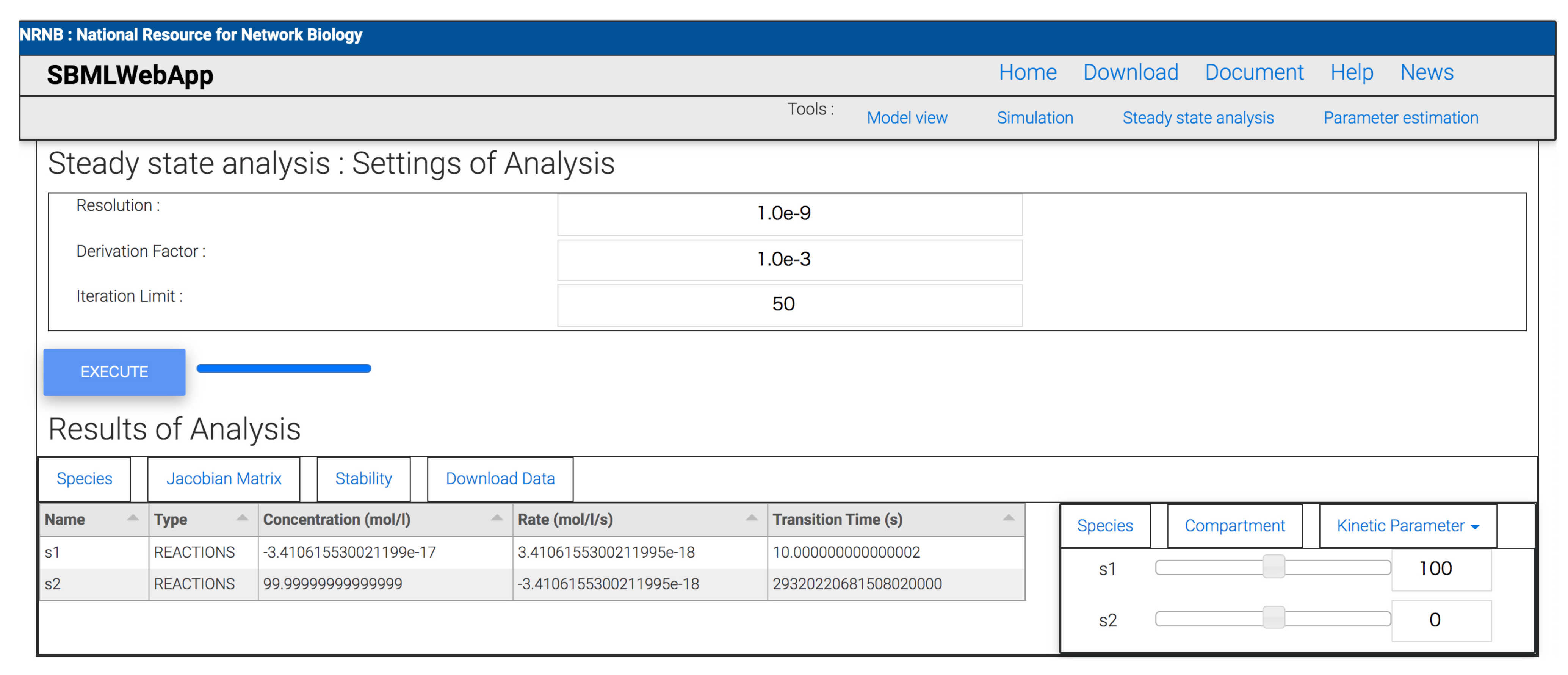
- steady-state analysis.
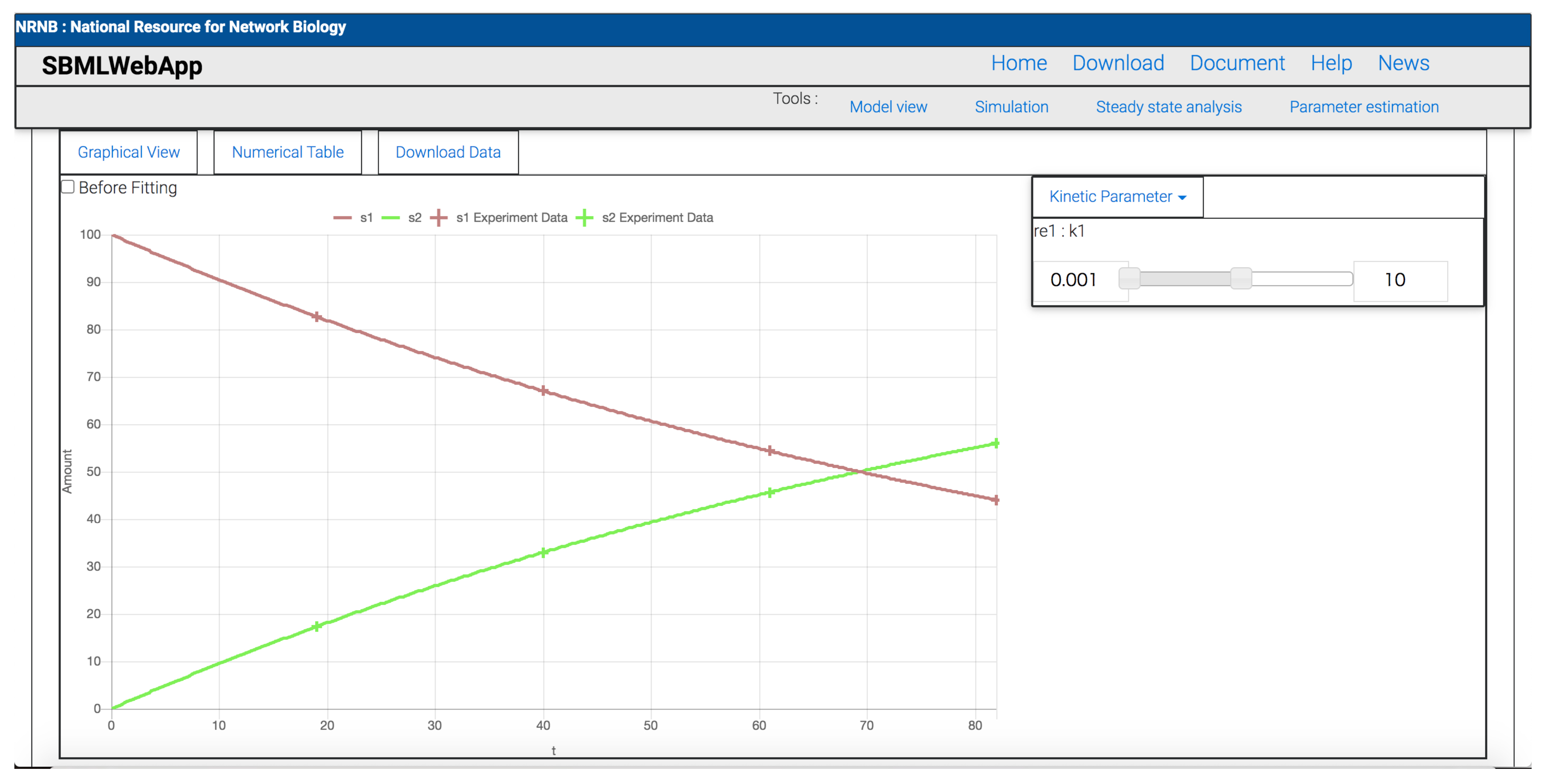
- parameter estimation.
2. Implementation
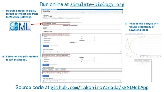
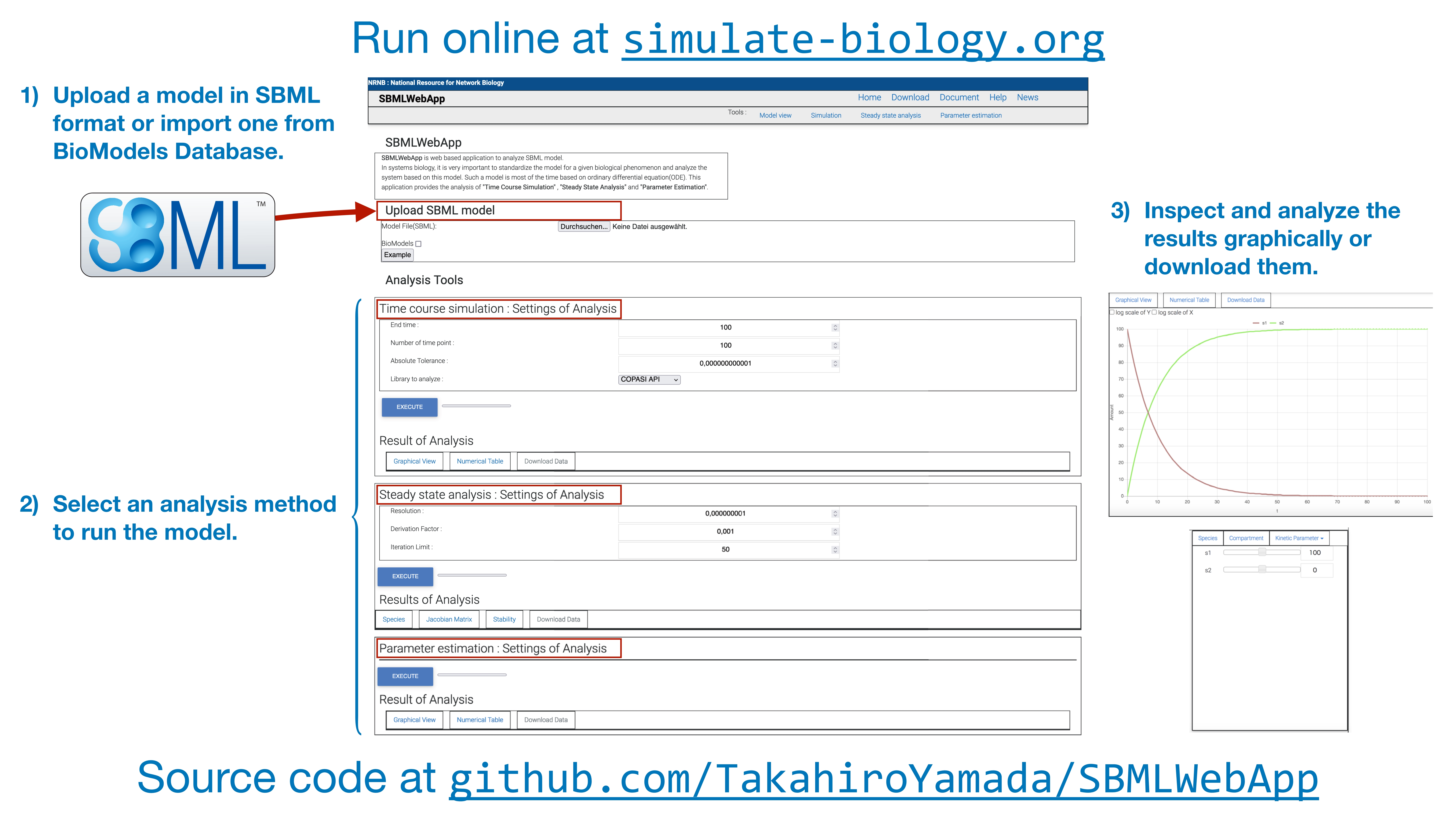
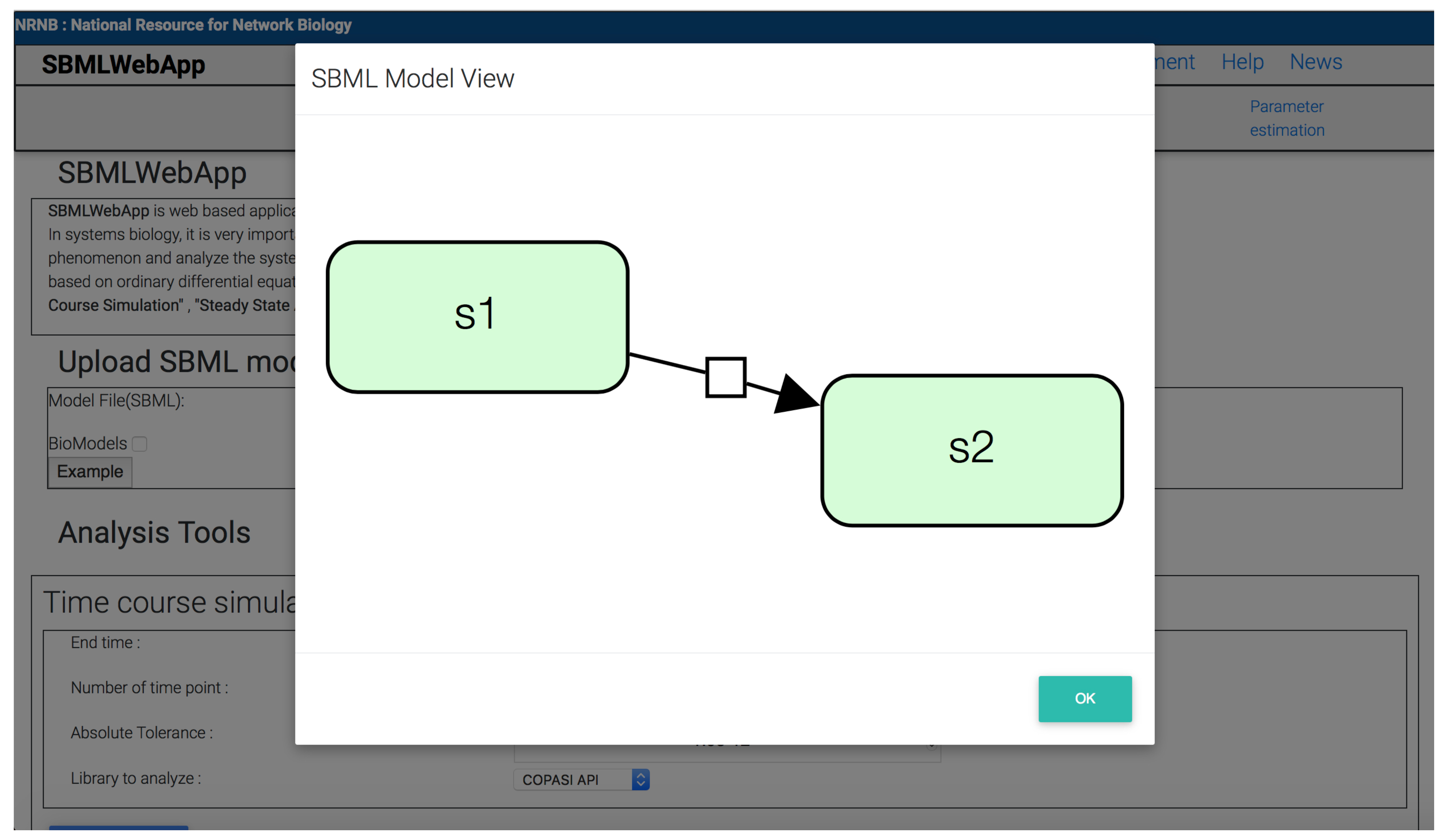
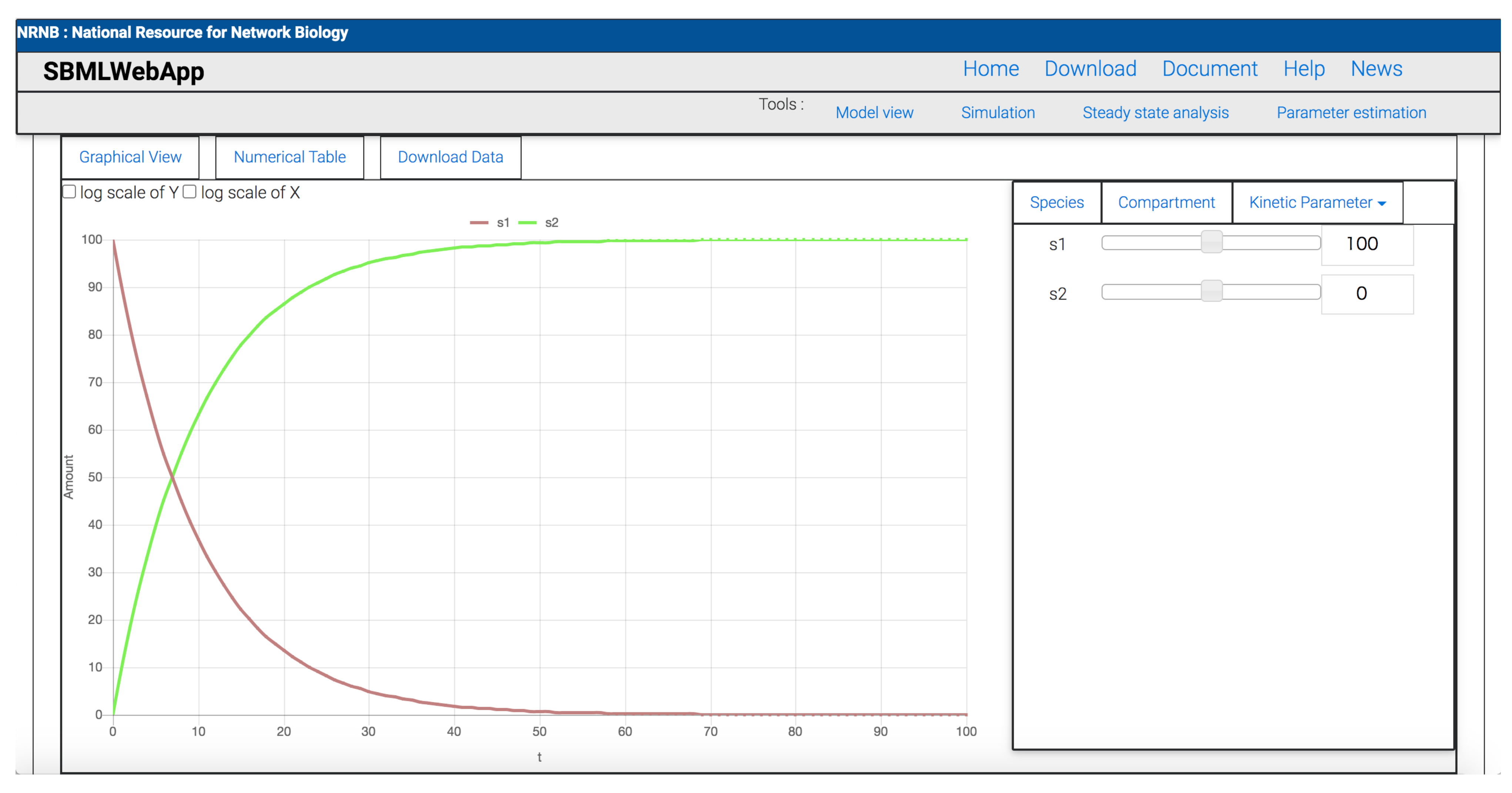
3. Using the SBMLWebApp
4. Real-World Example and Applications
5. Limitations of the Application
6. Conclusions
Supplementary Materials
Author Contributions
Funding
Institutional Review Board Statement
Informed Consent Statement
Data Availability Statement
Acknowledgments
Conflicts of Interest
Abbreviations
| CSV | Comma-Separated Values |
| COPASI | COmplex PAthway SImulator |
| GUI | Graphical User Interface |
| GWT | Google Web Toolkit |
| ODE | Ordinary Differential Equation |
| PE | Parameter Estimation |
| PNG | Portable Network Graphics |
| TCS | Time-Course Simulation |
| SBML | Systems Biology Markup Language |
| SBSCL | Systems Biology Simulation Core Library |
| SBW | Systems Biology Workbench |
| SSA | Steady-State Analysis |
References
- Kitano, H. Computational systems biology. Nature 2002, 420, 206–210. [Google Scholar] [CrossRef]
- Buchweitz, L.F.; Yurkovich, J.T.; Blessing, C.; Kohler, V.; Schwarzkopf, F.; King, Z.A.; Yang, L.; Jóhannsson, F.; Sigurjónsson, O.E.; Rolfsson, O.; et al. Visualizing metabolic network dynamics through time-series metabolomic data. BMC Bioinform. 2020, 21, 130. [Google Scholar] [CrossRef] [Green Version]
- Mienda, B.S.; Dräger, A. Genome-Scale Metabolic Modeling of Escherichia coli and Its Chassis Design for Synthetic Biology Applications. In Computational Methods in Synthetic Biology; Marchisio, M.A., Ed.; Humana Press: New York, NY, USA, 2020; Volume 2189, pp. 217–229. [Google Scholar] [CrossRef]
- Renz, A.; Widerspick, L.; Dräger, A. Genome-Scale Metabolic Model of Infection with SARS-CoV-2 Mutants Confirms Guanylate Kinase as Robust Potential Antiviral Target. Genes 2021, 12, 796. [Google Scholar] [CrossRef]
- Renz, A.; Widerspick, L.; Dräger, A. FBA reveals guanylate kinase as a potential target for antiviral therapies against SARS-CoV-2. Bioinformatics 2020, 36, i813–i821. [Google Scholar] [CrossRef]
- Mostolizadeh, R.; Dräger, A. Computational Model Informs Effective Control Interventions against Y. enterocolitica Co-Infection. Biology 2020, 9, 431. [Google Scholar] [CrossRef]
- Bauer, A.L.; Beauchemin, C.A.; Perelson, A.S. Agent-based modeling of host–pathogen systems: The successes and challenges. Inf. Sci. 2009, 179, 1379–1389. [Google Scholar] [CrossRef]
- Shinde, S.B.; Kurhekar, M.P. Review of the systems biology of the immune system using agent-based models. IET Syst. Biol. 2018, 12, 83–92. [Google Scholar] [CrossRef]
- Li, F.; Long, T.; Lu, Y.; Ouyang, Q.; Tang, C. The yeast cell-cycle network is robustly designed. Proc. Natl. Acad. Sci. USA 2004, 101, 4781–4786. [Google Scholar] [CrossRef] [PubMed] [Green Version]
- Chaouiya, C.; Bérenguier, D.; Keating, S.M.; Naldi, A.; van Iersel, M.P.; Rodriguez, N.; Dräger, A.; Büchel, F.; Cokelaer, T.; Kowal, B.; et al. SBML Qualitative Models: A model representation format and infrastructure to foster interactions between qualitative modelling formalisms and tools. BMC Syst. Biol. 2013, 7, 135. [Google Scholar] [CrossRef] [PubMed] [Green Version]
- Traynard, P.; Fauré, A.; Fages, F.; Thieffry, D. Logical model specification aided by model-checking techniques: Application to the mammalian cell cycle regulation. Bioinformatics 2016, 32, i772–i780. [Google Scholar] [CrossRef] [PubMed] [Green Version]
- Khatri, P.; Draghici, S.; Ostermeier, G.C.; Krawetz, S.A. Profiling gene expression using onto-express. Genomics 2002, 79, 266–270. [Google Scholar] [CrossRef] [Green Version]
- Supper, J.; Fröhlich, H.; Spieth, C.; Dräger, A.; Zell, A. Inferring Gene Regulatory Networks by Machine Learning Methods. In Proceedings of the 5th Asia-Pacific Bioinformatics Conference (APBC 2007), Hong Kong, China, 15–17 January 2007; Sankoff, D., Wang, L., Chin, F., Eds.; Series on Advances in Bioinformatics and Computational Biology. Imperial College Press: London, UK, 2007; Volume 5, pp. 247–256. [Google Scholar] [CrossRef] [Green Version]
- Renz, A.; Widerspick, L.; Dräger, A. First Genome-Scale Metabolic Model of Dolosigranulum pigrum Confirms Multiple Auxotrophies. Metabolites 2021, 11, 232. [Google Scholar] [CrossRef]
- Erhard, F.; Friedel, C.C.; Zimmer, R. FERN – a Java framework for stochastic simulation and evaluation of reaction networks. BMC Bioinform. 2008, 9, 356. [Google Scholar] [CrossRef] [Green Version]
- Smallbone, K.; Simeonidis, E.; Swainston, N.; Mendes, P. Towards a genome-scale kinetic model of cellular metabolism. BMC Syst. Biol. 2010, 4, 1–9. [Google Scholar] [CrossRef] [PubMed] [Green Version]
- Karr, J.R.; Sanghvi, J.C.; Macklin, D.N.; Gutschow, M.V.; Jacobs, J.M.; Bolival, B., Jr.; Assad-Garcia, N.; Glass, J.I.; Covert, M.W. A whole-cell computational model predicts phenotype from genotype. Cell 2012, 150, 389–401. [Google Scholar] [CrossRef] [PubMed] [Green Version]
- Strutz, J.; Martin, J.; Greene, J.; Broadbelt, L.; Tyo, K. Metabolic kinetic modeling provides insight into complex biological questions, but hurdles remain. Curr. Opin. Biotechnol. 2019, 59, 24–30. [Google Scholar] [CrossRef] [PubMed]
- Tummler, K.; Klipp, E. The discrepancy between data for and expectations on metabolic models: How to match experiments and computational efforts to arrive at quantitative predictions? Curr. Opin. Syst. Biol. 2018, 8, 1–6. [Google Scholar] [CrossRef]
- Resat, H.; Petzold, L.; Pettigrew, M.F. Kinetic modeling of biological systems. Comput. Syst. Biol. 2009, 311–335. [Google Scholar] [CrossRef] [Green Version]
- Klipp, E.; Nordlander, B.; Krüger, R.; Gennemark, P.; Hohmann, S. Integrative model of the response of yeast to osmotic shock. Nat. Biotechnol. 2005, 23, 975–982. [Google Scholar] [CrossRef]
- Du, B.; Zielinski, D.; Dräger, A.; Tan, J.; Zhang, Z.; Ruggiero, K.; Arzumanyan, G.; Palsson, B.O. Evaluation of Rate Law Approximations in Bottom-up Kinetic Models of Metabolism. BMC Syst. Biol. 2016, 10, 1–15. [Google Scholar] [CrossRef] [Green Version]
- Chowdhury, A.; Khodayari, A.; Maranas, C.D. Improving prediction fidelity of cellular metabolism with kinetic descriptions. Curr. Opin. Biotechnol. 2015, 36, 57–64. [Google Scholar] [CrossRef] [Green Version]
- Mendes, P.; Kell, D. Non-linear optimization of biochemical pathways: Applications to metabolic engineering and parameter estimation. Bioinformatics 1998, 14, 869–883. [Google Scholar] [CrossRef] [Green Version]
- Renz, A.; Mostolizadeh, R.; Dräger, A. Clinical Applications of Metabolic Models in SBML Format. In Systems Medicine; Wolkenhauer, O., Ed.; Academic Press: Oxford, UK, 2020; Volume 3, pp. 362–371. [Google Scholar] [CrossRef]
- Keating, S.M.; Waltemath, D.; König, M.; Zhang, F.; Dräger, A.; Chaouiya, C.; Bergmann, F.T.; Finney, A.; Gillespie, C.S.; Helikar, T.; et al. SBML Level 3: An extensible format for the exchange and reuse of biological models. Mol. Syst. Biol. 2020, 16, e9110. [Google Scholar] [CrossRef]
- Hoops, S.; Sahle, S.; Gauges, R.; Lee, C.; Pahle, J.; Simus, N.; Kummer, U. COPASI—a complex pathway simulator. Bioinformatics 2006, 22, 3067–3074. [Google Scholar] [CrossRef] [Green Version]
- Schmidt, H.; Jirstrand, M. Systems Biology Toolbox for MATLAB: A computational platform for research in systems biology. Bioinformatics 2006, 22, 514–515. [Google Scholar] [CrossRef] [Green Version]
- Somogyi, E.T.; Bouteiller, J.M.; Glazier, J.A.; König, M.; Medley, J.K.; Swat, M.H.; Sauro, H.M. libRoadRunner: A high performance SBML simulation and analysis library. Bioinformatics 2015, 31, 3315–3321. [Google Scholar] [CrossRef] [Green Version]
- Dörr, A.; Keller, R.; Zell, A.; Dräger, A. SBMLsimulator: A Java tool for model simulation and parameter estimation in systems biology. Computation 2014, 2, 246–257. [Google Scholar] [CrossRef] [PubMed] [Green Version]
- Hedengren, J.D.; Shishavan, R.A.; Powell, K.M.; Edgar, T.F. Nonlinear modeling, estimation and predictive control in APMonitor. Comput. Chem. Eng. 2014, 70, 133–148. [Google Scholar] [CrossRef] [Green Version]
- Le Fèvre, F.; Smidtas, S.; Combe, C.; Durot, M.; d’Alché-Buc, F.; Schachter, V. CycSim—An online tool for exploring and experimenting with genome-scale metabolic models. Bioinformatics 2009, 25, 1987–1988. [Google Scholar] [CrossRef] [PubMed] [Green Version]
- Bergmann, F.T.; Sauro, H.M. SBW-a modular framework for systems biology. In Proceedings of the 2006 Winter Simulation Conference, Monterey, CA, USA, 3–6 December 2006; pp. 1637–1645. [Google Scholar]
- Olivier, B.G.; Snoep, J.L. Web-based kinetic modelling using JWS Online. Bioinformatics 2004, 20, 2143–2144. [Google Scholar] [CrossRef] [PubMed]
- Shaikh, B.; Marupilla, G.; Wilson, M.; Blinov, M.L.; Moraru, I.I.; Karr, J.R. RunBioSimulations: An extensible web application that simulates a wide range of computational modeling frameworks, algorithms, and formats. Nucleic Acids Res. 2021, 49, W597–W602. [Google Scholar] [CrossRef]
- Keller, R.; Dörr, A.; Tabira, A.; Funahashi, A.; Ziller, M.J.; Adams, R.; Rodriguez, N.; Le Novère, N.; Hiroi, N.; Planatscher, H.; et al. The systems biology simulation core algorithm. BMC Syst. Biol. 2013, 7, 55. [Google Scholar] [CrossRef] [Green Version]
- Panchiwala, H.; Shah, S.; Planatscher, H.; Zakharchuk, M.; König, M.; Dräger, A. The Systems Biology Simulation Core Library. Bioinformatics 2021, btab669. [Google Scholar] [CrossRef]
- Rodriguez, N.; Thomas, A.; Watanabe, L.; Vazirabad, I.Y.; Kofia, V.; Gómez, H.F.; Mittag, F.; Matthes, J.; Rudolph, J.D.; Wrzodek, F.; et al. JSBML 1.0: Providing a smorgasbord of options to encode systems biology models. Bioinformatics 2015, 31, 3383–3386. [Google Scholar] [CrossRef]
- Takizawa, H.; Nakamura, K.; Tabira, A.; Chikahara, Y.; Matsui, T.; Hiroi, N.; Funahashi, A. LibSBMLSim: A reference implementation of fully functional SBML simulator. Bioinformatics 2013, 29, 1474–1476. [Google Scholar] [CrossRef] [Green Version]
- Bornstein, B.J.; Keating, S.M.; Jouraku, A.; Hucka, M. LibSBML: An API Library for SBML. Bioinformatics 2008, 24, 880–881. [Google Scholar] [CrossRef] [PubMed]
- Hucka, M.; Bergmann, F.T.; Dräger, A.; Hoops, S.; Keating, S.M.; Le Novère, N.; Myers, C.J.; Olivier, B.G.; Sahle, S.; Schaff, J.C.; et al. Systems Biology Markup Language (SBML) Level 3 Version 1 Core. J. Integr. Bioinform. 2018, 15, 1. [Google Scholar] [CrossRef] [Green Version]
- Malik-Sheriff, R.S.; Glont, M.; Nguyen, T.V.N.; Tiwari, K.; Roberts, M.G.; Xavier, A.; Vu, M.T.; Men, J.; Maire, M.; Kananathan, S.; et al. BioModels—15 years of sharing computational models in life science. Nucleic Acids Res. 2020, 48, D407–D415. [Google Scholar] [CrossRef] [Green Version]
- Franz, M.; Lopes, C.T.; Huck, G.; Dong, Y.; Sumer, O.; Bader, G.D. Cytoscape. js: A graph theory library for visualisation and analysis. Bioinformatics 2015, 32, 309–311. [Google Scholar]
- Levenberg, K. A method for the solution of certain non-linear problems in least squares. Q. Appl. Math. 1944, 2, 164–168. [Google Scholar] [CrossRef] [Green Version]
- Marquardt, D.W. An algorithm for least-squares estimation of nonlinear parameters. J. Soc. Ind. Appl. Math. 1963, 11, 431–441. [Google Scholar] [CrossRef]
- Nelder, J.A.; Mead, R. A simplex method for function minimization. Comput. J. 1965, 7, 308–313. [Google Scholar] [CrossRef]
- Kennedy, J.; Eberhart, R. Particle swarm optimization. In Proceedings of the ICNN’95-International Conference on Neural Networks, Perth, WA, Australia, 27 November–27 December 1995; Volume 4, pp. 1942–1948. [Google Scholar]
- Storn, R.; Price, K. Differential evolution—A simple and efficient heuristic for global optimization over continuous spaces. J. Glob. Optim. 1997, 11, 341–359. [Google Scholar] [CrossRef]
- Dräger, A.; Kronfeld, M.; Ziller, M.J.; Supper, J.; Planatscher, H.; Magnus, J.B.; Oldiges, M.; Kohlbacher, O.; Zell, A. Modeling metabolic networks in C. glutamicum: A comparison of rate laws in combination with various parameter optimization strategies. BMC Syst. Biol. 2009, 3, 5. [Google Scholar] [CrossRef] [Green Version]
- Perelson, A.S.; Kirschner, D.E.; De Boer, R. Dynamics of HIV infection of CD4+ T cells. Math. Biosci. 1993, 114, 81–125. [Google Scholar] [CrossRef] [Green Version]
- Stafford, M.A.; Corey, L.; Cao, Y.; Daar, E.S.; Ho, D.D.; Perelson, A.S. Modeling Plasma Virus Concentration during Primary HIV Infection. J. Theor. Biol. 2000, 203, 285–301. [Google Scholar] [CrossRef] [PubMed] [Green Version]
- Carey, M.A.; Dräger, A.; Beber, M.E.; Papin, J.A.; Yurkovich, J.T. Community standards to facilitate development and address challenges in metabolic modeling. Mol. Syst. Biol. 2020, 16, e9235. [Google Scholar] [CrossRef] [PubMed]
- Hucka, M.; Bergmann, F.T.; Hoops, S.; Keating, S.M.; Sahle, S.; Schaff, J.C.; Smith, L.P.; Wilkinson, D.J. The Systems Biology Markup Language (SBML): Language specification for level 3 version 1 core. J. Integr. Bioinform. 2015, 12, 382–549. [Google Scholar] [CrossRef] [Green Version]
- Funahashi, A.; Morohashi, M.; Kitano, H.; Tanimura, N. CellDesigner: A process diagram editor for gene-regulatory and biochemical networks. Biosilico 2003, 1, 159–162. [Google Scholar] [CrossRef]
- Funahashi, A.; Matsuoka, Y.; Jouraku, A.; Morohashi, M.; Kikuchi, N.; Kitano, H. CellDesigner 3.5: A versatile modeling tool for biochemical networks. Proc. IEEE 2008, 96, 1254–1265. [Google Scholar] [CrossRef]
- Bergmann, F.T.; Hoops, S.; Klahn, B.; Kummer, U.; Mendes, P.; Pahle, J.; Sahle, S. COPASI and its applications in biotechnology. J. Biotechnol. 2017, 261, 215–220. [Google Scholar] [CrossRef] [PubMed]


| Model | Authors | File Size | Run Time TCS | Run Time SSA | Run Time PE |
|---|---|---|---|---|---|
| See Supplement | Perelson et al. | 43.16 kB | 623.5 ms | 346.7 ms | 14,180.7 ms |
Publisher’s Note: MDPI stays neutral with regard to jurisdictional claims in published maps and institutional affiliations. |
© 2021 by the authors. Licensee MDPI, Basel, Switzerland. This article is an open access article distributed under the terms and conditions of the Creative Commons Attribution (CC BY) license (https://creativecommons.org/licenses/by/4.0/).
Share and Cite
Yamada, T.G.; Ii, K.; König, M.; Feierabend, M.; Dräger, A.; Funahashi, A. SBMLWebApp: Web-Based Simulation, Steady-State Analysis, and Parameter Estimation of Systems Biology Models. Processes 2021, 9, 1830. https://0-doi-org.brum.beds.ac.uk/10.3390/pr9101830
Yamada TG, Ii K, König M, Feierabend M, Dräger A, Funahashi A. SBMLWebApp: Web-Based Simulation, Steady-State Analysis, and Parameter Estimation of Systems Biology Models. Processes. 2021; 9(10):1830. https://0-doi-org.brum.beds.ac.uk/10.3390/pr9101830
Chicago/Turabian StyleYamada, Takahiro G., Kaito Ii, Matthias König, Martina Feierabend, Andreas Dräger, and Akira Funahashi. 2021. "SBMLWebApp: Web-Based Simulation, Steady-State Analysis, and Parameter Estimation of Systems Biology Models" Processes 9, no. 10: 1830. https://0-doi-org.brum.beds.ac.uk/10.3390/pr9101830