Digital Twins for Continuous mRNA Production

Abstract

The global coronavirus pandemic continues to restrict public life worldwide. An effective means of limiting the pandemic is vaccination. Messenger ribonucleic acid (mRNA) vaccines currently available on the market have proven to be a well-tolerated and effective class of vaccine against coronavirus type 2 (CoV2). Accordingly, demand is presently outstripping mRNA vaccine production. One way to increase productivity is to switch from the currently performed batch to continuous in vitro transcription, which has proven to be a crucial material-consuming step. In this article, a physico-chemical model of in vitro mRNA transcription in a tubular reactor is presented and compared to classical batch and continuous in vitro transcription in a stirred tank. The three models are validated based on a distinct and quantitative validation workflow. Statistically significant parameters are identified as part of the parameter determination concept. Monte Carlo simulations showed that the model is precise, with a deviation of less than 1%. The advantages of continuous production are pointed out compared to batchwise in vitro transcription by optimization of the space–time yield. Improvements of a factor of 56 (0.011 µM/min) in the case of the continuously stirred tank reactor (CSTR) and 68 (0.013 µM/min) in the case of the plug flow reactor (PFR) were found.

1. Introduction

In the past 1.5 years, mRNA-based vaccines have become increasingly relevant due to the COVID-19 pandemic. In contrast to classical vaccines, which use a protein or inactivated virus to stimulate the immune response, mRNA-based vaccines introduce the protein-coding information in the form of mRNA directly into the patient’s cells, causing them to produce the antigen themselves [1,2,3]. In contrast to deoxyribonucleic acid (DNA)-based vaccines, this form of vaccination offers the advantage that no alteration of the recipient genome can be altered by recombination events [4,5]. Two of the first vaccines against SARS-CoV-2 approved in Europe and the United States were mRNA-based vaccines [6,7]. The state of the art of industrial production of this class of vaccines is based on so-called in vitro transcription, which is an enzymatically catalyzed reaction [8]. Against the background of the dynamic pandemic situation, this process, which is carried out in batches, has limitations in terms of scale and the associated production capacity [9]. A switch to continuous production, as also demanded by the European Medical Association [10] and Food and Drug Administration [11], is to be aimed at, due to the advantages in agility, flexibility, quality, and costs [12]. The control strategy to be developed in the context of a quality-by-design (QbD)-based process development, to ensure the quality target product profile (QTPP), requires design spaces [13]. These can be defined via validated process models in order to avoid out-of specification (OOS) batches [14,15]. On the other hand, advanced process control can be realized on the basis of a validated process model developed digital twin [16]. Although basic research on the fundamental processes of in vitro transcription can be found, to our knowledge there is no publication of a digital twin for continuous in vitro transcription that explicitly addresses QbD-compliant model validation and the requirements for a digital twin in good manufacturing process (GMP)-compliant production. The aim of this work is therefore to fill this critical gap, in which distinct and quantitative criteria for assessing validity and suitability as a predictive process model and digital twin are demonstrated. In addition, the extensive studies are used to quantify the advantages in terms of space–time yield, representative of speed and capacity, of continuous production over a batchwise production. Furthermore, these results have been incorporated into an extensive study comparing batchwise and continuous total processes in a recently published paper and could be used to determine the optimal operating points for in vitro transcription. The presented digital twins lay the foundation for future experimental validation.

1.1. State of the Art of IVT

In vitro transcription describes an enzymatic reaction in which mRNA is produced from template DNA. Traditionally, T7, SP6, or T3 RNA polymerase are used as enzymes that act as catalysts for the reaction. In addition to the enzyme, nucleotides are required as substrates for in vitro transcription, as well as MgCl₂ as a cofactor of the polymerase. The reaction scheme was adapted from the literature considering the in vitro transcription by T7 RNA polymerase [17]. The reaction is divided into the following reaction steps: initiation (Equations (1)–(5)), elongation (Equation (6)), and termination (Equation (13)) [17,18,19]. Dot signs refer to a bound complex of the indicated components.

Reversible reactions are described by equilibrium constants K_i, whereas irreversible reactions are characterised by rate constants k_I, k_E, and k_T. The initiation step of in vitro transcription is described in this work using a mechanism that considers both the random binding of the first nucleotide, GTP, and that of the promoter (D) located on the DNA template. Initiation is completed with the irreversible formation of an enzyme–DNA–RNA complex, which is described by E∙D∙Mj. The elongation of the mRNA occurs when a nucleotide (ATP, CTP, GTP, UTP; summarized as NTP) is reversibly bound by the enzyme (E) and forms a complex together with the DNA and the already formed RNA. Through an irreversible reaction, the nucleotide is bound to the RNA and an inorganic pyrophosphate (PPi) is cleaved off. Nucleotides can bind to the free enzyme, to the promoter–enzyme complex, and to the transcription complex. This leads to a competitive situation and consequently to competitive inhibition (Equations (7)–(12)). In addition, the resulting pyrophosphate has a negative influence on the transcription rate because it can temporarily bind to the nucleotide binding site of both the freely soluble T7 RNA polymerase and the enzyme–DNA–RNA complex [17,20,21]. Once the mRNA has reached its final length, the transcription complex spontaneously dissolves, releasing the mRNA product (M_n) and leaving both the enzyme and the template DNA unbound [17].

Initiation:

$$\mathrm{E}+\mathrm{GTP}\stackrel{{\mathrm{K}}_{\mathrm{G}}^{\mathrm{I}}}{ \overbrace{\rightleftharpoons }}\mathrm{E}·\mathrm{GTP}$$

(1)

$$\mathrm{E}+\mathrm{D}\stackrel{{\mathrm{K}}_{\mathrm{D}}}{\overbrace{\rightleftharpoons }}\mathrm{E}·\mathrm{D}$$

(2)

$$\mathrm{E}·\mathrm{GTP}+\mathrm{D}\stackrel{{\mathrm{K}}_{\mathrm{D}}}{\overbrace{\rightleftharpoons }}\mathrm{E}·\mathrm{GTP}·\mathrm{D}$$

(3)

$$\mathrm{E}·\mathrm{D}+\mathrm{GTP}\stackrel{{\mathrm{K}}_{\mathrm{G}}^{\mathrm{I}}}{ \overbrace{\rightleftharpoons }}\mathrm{E}·\mathrm{D}·\mathrm{GTP}$$

(4)

$$\mathrm{E}·\mathrm{D}·\mathrm{GTP}\stackrel{{\mathrm{k}}_{\mathrm{I}}}{\overbrace{\to }}\mathrm{E}·\mathrm{D}·{\mathrm{M}}_1$$

(5)

Elongation:

$$\mathrm{E}·\mathrm{D}·{\mathrm{M}}_j+\mathrm{NTP}\stackrel{{\mathrm{K}}_{\mathrm{N}\mathrm{T}\mathrm{P}}}{\overbrace{\rightleftharpoons }}\mathrm{E}·\mathrm{D}·{\mathrm{M}}_j·\mathrm{NTP}\stackrel{{\mathrm{K}}_{\mathrm{E}}}{\overbrace{\to }}\mathrm{E}·\mathrm{D}·{\mathrm{M}}_{j+1}+{\mathrm{PP}}_{\mathrm{i}}$$

(6)

Competitive Inhibition:

$$\mathrm{E}+\mathrm{NTP}\stackrel{{\mathrm{K}}_{\mathrm{I} \mathrm{N}\mathrm{T}\mathrm{P}}}{\overbrace{\rightleftharpoons }}\mathrm{E}·\mathrm{NTP}$$

(7)

$$\mathrm{E}·\mathrm{D}+\mathrm{NTP}\stackrel{{\mathrm{K}}_{\mathrm{I} \mathrm{N}\mathrm{T}\mathrm{P}}}{\overbrace{\rightleftharpoons }}\mathrm{E}·\mathrm{D}·\mathrm{NTP}$$

(8)

$$\mathrm{E}+{\mathrm{PP}}_{\mathrm{i}}\stackrel{{\mathrm{K}}_{\mathrm{I} \mathrm{P}\mathrm{P}\mathrm{i}}}{\overbrace{\rightleftharpoons }}\mathrm{E}·{\mathrm{PP}}_{\mathrm{i}}$$

(9)

$$\mathrm{E}·\mathrm{D}+{\mathrm{PP}}_{\mathrm{i}}\stackrel{{\mathrm{K}}_{\mathrm{I} \mathrm{P}\mathrm{P}\mathrm{i}}}{\overbrace{\rightleftharpoons }}\mathrm{E}·\mathrm{D}·{\mathrm{PP}}_{\mathrm{i}}$$

(10)

$$\mathrm{E}·\mathrm{D}·{\mathrm{M}}_j+\mathrm{NTP}\stackrel{{\mathrm{K}}_{\mathrm{I} \mathrm{N}\mathrm{T}\mathrm{P}}}{\overbrace{\rightleftharpoons }}\mathrm{E}·\mathrm{D}·{\mathrm{M}}_j·\mathrm{NTP}$$

(11)

$$\mathrm{E}·\mathrm{D}·{\mathrm{M}}_j+{\mathrm{PP}}_{\mathrm{i}}\stackrel{{\mathrm{K}}_{\mathrm{I} \mathrm{P}\mathrm{P}\mathrm{i}}}{\overbrace{\rightleftharpoons }}\mathrm{E}·\mathrm{D}·{\mathrm{M}}_j·{\mathrm{PP}}_{\mathrm{i}}$$

(12)

Termination:

$$\mathrm{E}·\mathrm{D}·{\mathrm{M}}_n\stackrel{{\mathrm{k}}_{\mathrm{T}}}{\overbrace{\rightleftharpoons }}\mathrm{E}+\mathrm{D}+{\mathrm{M}}_n$$

(13)

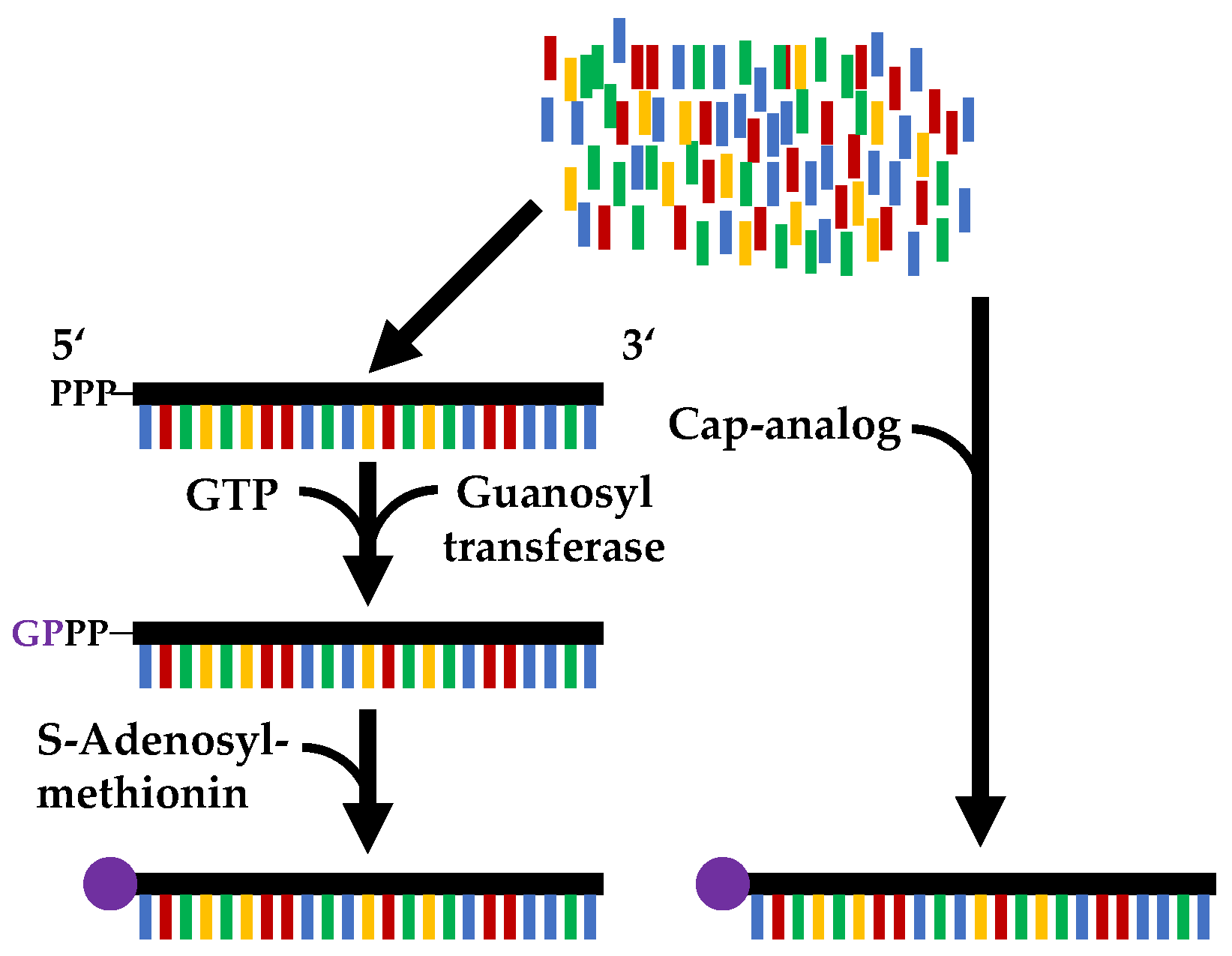
To prevent the degradation of the mRNA in vivo it must be capped. This can be achieved either co-transcriptionally, i.e., during the in vitro transcription, or post-transcriptionally in a subsequent process step. The reaction schemes of the two capping mechanisms are shown in Figure 1. In co-transcriptional capping, the mRNA is capped by the polymerase through the addition of a cap analogue. Post-transcriptional capping is performed as a second enzymatic reaction, using the vaccinia capping enzyme [22,23,24].

Post-transcriptional capping takes place in three successive reaction steps. First, the γ-phosphate of the mRNA is hydrolysed with the help of a 5′-triphosphatase. Guanylyltransferase then transfers GMP derived from the substrate GTP to form the 5′-5′-linked Gppp RNA. Finally, methylation occurs when an RNA (guanine-N7) methyltransferase methylates the mRNA with the co-substrate S-adenosyl-L-methionine (AdoMet) [25,26,27].

In contrast to post-transcriptional capping, co-transcriptional capping takes place during in vitro transcription in a single reaction step. This is catalysed by the polymerase used, which transfers the added cap analogue to the 5′ end of the mRNA. The cap analogues are not incorporated into the mRNA during in vitro transcription because they lack a free 5′-triphosphate, such that they are only incorporated at the 5′-end of the mRNA. m7GpppG is most frequently used as a cap analogue [27,28]. One problem with co-transcriptional capping is that elongation occurs in the “wrong” direction, at the 3′-OH of the cap analogue, resulting in mRNA with the cap in reverse orientation, which means it cannot be translated [27,29]. One possible solution is to use anti-reverse cap analogues (ARCA) or m7pppG modified at the 2’ position [27,30,31,32]. Another problem of co-transcriptional capping is that the cap analogue competes with GTP as an initiator of in vitro transcription, resulting in not all of the mRNA being capped [27]. This results in a capping efficiency of 60–80%, in contrast to approx. 100% for post-transcriptional capping. The latter, however, has to catalyse three reactions instead of only one, which results in a longer production time [1,22].

Since the costs of the input materials for in vitro transcription capping, especially the cap analogue and the enzyme, account for most of the production costs, it makes sense to switch the process from batch to continuous [9]. In this way, the use of cost-intensive reagents can be reduced and, by using in situ product removal as well as substrate feed and product recovery strategies, molecules such as enzymes, co-factors, or nucleotides can be easily separated and returned to the process [22,34].

1.2. QbD-Based Process Development

QbD-based process development can be used to establish causality between process parameters and the relevant quality attributes of the product. The holistic QbD approach can ensure consistent product quality from development through piloting to production, and is also applied in other pharmaceutical manufacturing applications [15,35]. Process models can be used for the real-time prediction of quality attributes and their development during the process. Thus, when optimising the process, changes to it are possible even after submission. To achieve this, a digital representation of the process is needed, also called a “Digital Twin” (DT).

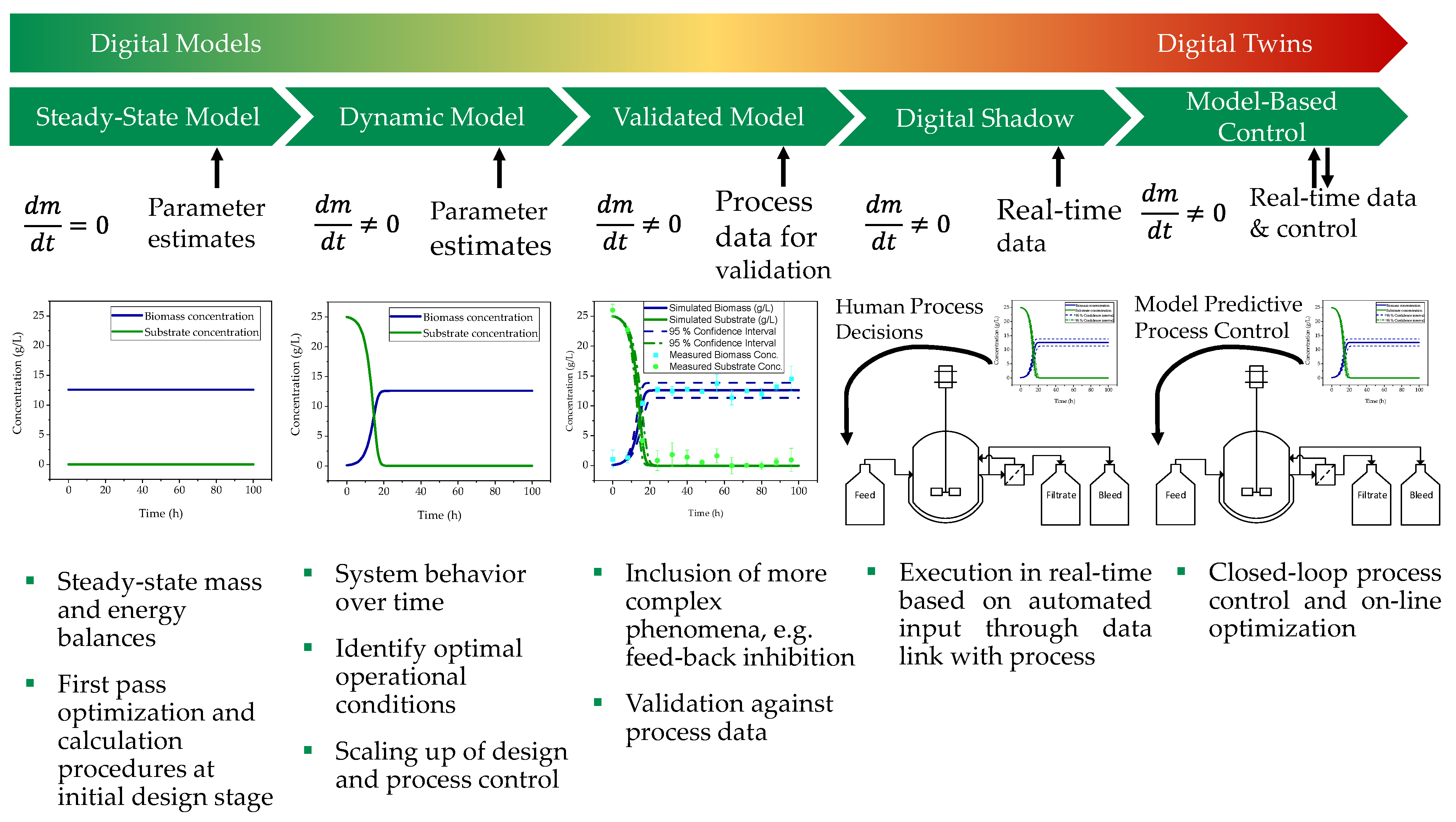
A Digital Twin can be divided into five levels (cf. Figure 2), whereby the first three levels reflect purely digital models, and the level of detail increases per level. The first step consists of a steady-state model that describes the process with the help of time-independent mass and energy balances. This is used in the first design phase of the process for initial optimisation and calculation procedures [36,37,38,39]. If the steady-state model is extended by accumulation terms and the system dynamics, the second stage of a digital twin is reached. This is a dynamic model that becomes time dependent through the time derivative of all variables of interest. It is used for the identification of optimal operational conditions, scaling-up design, and process control [36,40,41,42]. The final stage of a purely digital model is the validated model, which must be validated against process data. This extends the capabilities of the dynamic process model by considering phenomena such as inhibition, which increases the number of states. It also includes equipment constraint terms such as working capacity and hydraulics. The penultimate step to a complete digital twin is the digital shadow. This is a validated model that can be executed in real time based on automatic inputs via a data link with the physical process. Model-based control is the final stage of a digital twin and involves closed-loop control. It also enables online optimisation of the process. The digitalisation infrastructure enables the implementation of control structures based on the model-based predictions [36].

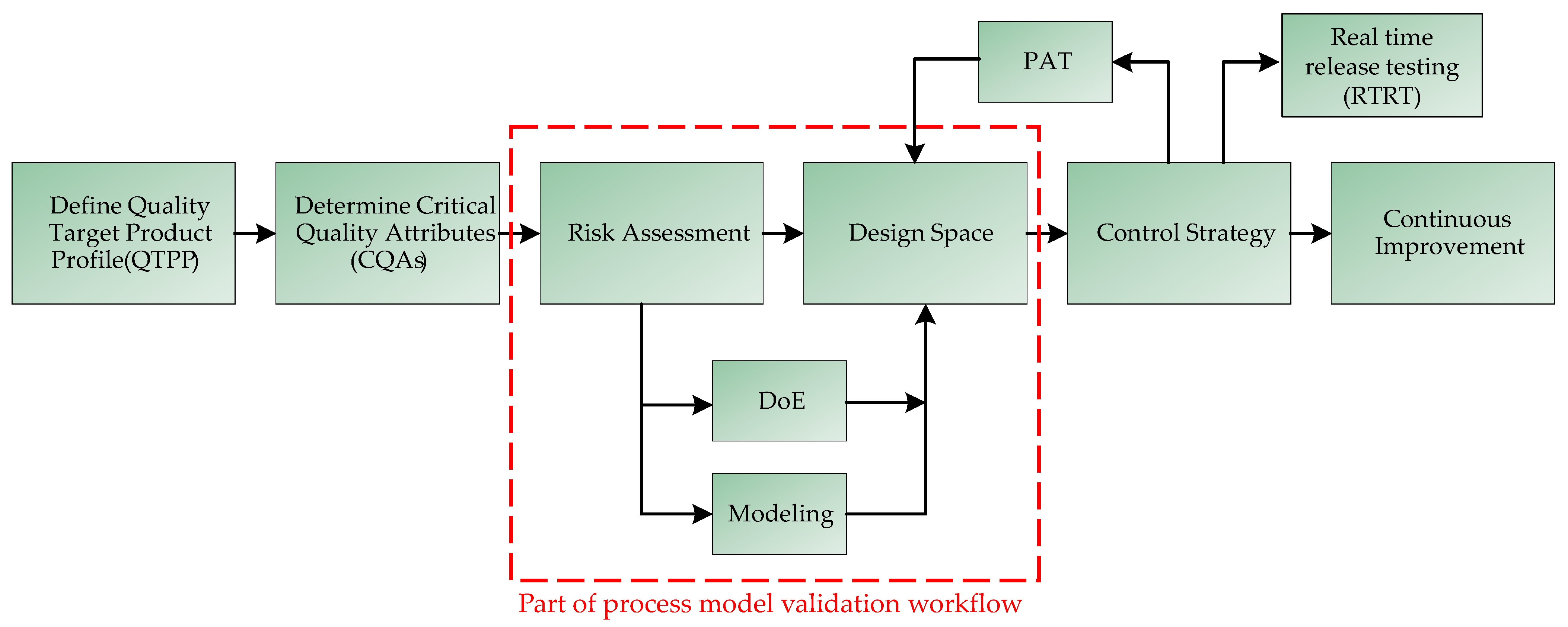
QbD is based on a validated design space in which consistent quality can be ensured and which can be spanned through experimentation or by rigorous process models. The workflow for developing a QbD process is shown in Figure 3 [43,44].

First, the definition of a quality target product profile (QTPP) is necessary. The QTPP is related to the quality, safety, and efficacy of the active ingredient, as the QTPPs may affect the bioavailability, the strength of the effect, and the stability of the active ingredient [45]. Characteristics that, when controlled within a certain limit, range, or distribution, lead to the desired product quality are called critical quality attributes (CQAs) and must be defined and ranked [46,47,48].

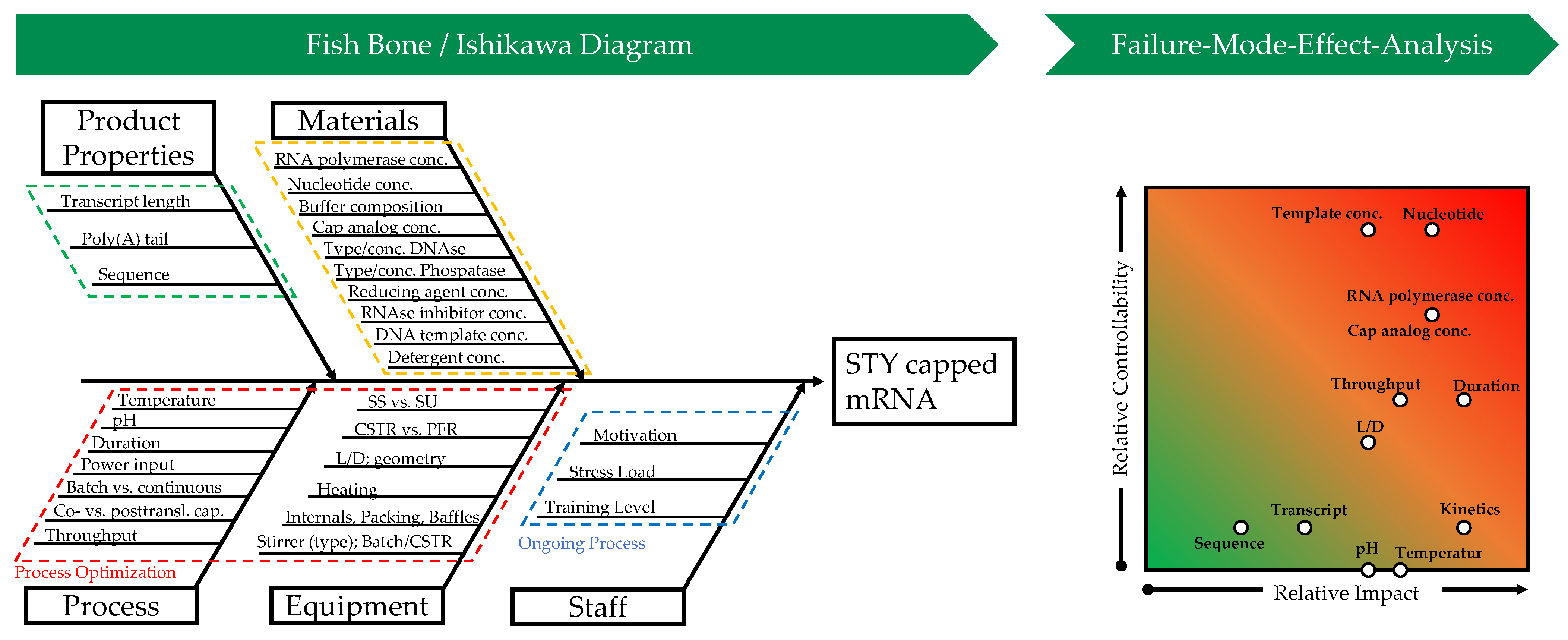
CQAs are the basis for further process development and need to be dynamically adapted as new knowledge is gained about the process or product. They are obtained through experimentation and risk management, the latter including risk assessment, which should be carried out at the beginning of process development. It serves to define the scope for process design by identifying relationships, known and hypothetical, between material, equipment, and process parameters and CQAs. The risk assessment can be carried out with the help of the Ishikawa analysis, which is shown in Figure 4 [48,49].

On the main branches, in the Ishikawa diagram, the effects, such as material properties, equipment design, and process parameters, which can affect CQAs, such as yield, purity, or generally the process capability, are shown. To obtain a more detailed description of the relationship between cause and risk, the main branches are further broken down into subsidiary branches. The prior knowledge gathered by the process development team determines the level of detail in the diagram. The Ishikawa diagram can be used to determine critical process parameters (CPPs) and the limits within which they must be maintained during the process. CPPs should consequently be part of the process control strategy [48].

In

Table 1. Failure mode effect analysis (FMEA) of key process parameters in in vitro transcription. The severity and the probability of occurrence are multiplied together, resulting in a risk score. This determines whether a parameter must be investigated by univariate (UV) or multivariate (MV) analysis as part of the model validation procedure. Colors indicate risk scores from low (gray, green) to medium (yellow) to high (red).

Risk	Severity	Occurrence	Risk Score	Characterization
Transcript length	5	1	5	UV	For a product not variable. Relevant for process change for product changeover.
Sequence	3	1	3	UV	For a product not variable. Relevant for process change for product changeover.
RNA polymerase concentration	9	6	54	MV	Influences kinetics and is therefore important for process optimization. Can be freely selected within the economic limits of the design space.
Nucleotide concentration	9	8	72	MV	Influences kinetics and is therefore important for process optimization. Can be freely selected within the economic limits of the design space.
Cap analogue concentration	9	6	54	MV	Influences kinetics and is therefore important for process optimization. Can be freely selected within the economic limits of the design space.
Template concentration	7	8	56	MV	Influences kinetics and is therefore important for process optimization. Can be freely selected within the economic limits of the design space.
Duration	10	4	40	MV	Great influence on hydrodynamics (back-mixing, flow regime, residence time)
Throughput	8	4	32	MV	Great influence on hydrodynamics (back-mixing, flow regime, residence time)
L/D	7	3	21	MV	Great influence on hydrodynamics (back-mixing, flow regime, etc.)
Kinetics	10	1	10	UV	Primarily based on Michaelis constants, can be the subject of imprecise determination
Temperature	8	0	0	X	Severely impacts kinetics/enzyme stability, can be easily controlled at the known optimum
pH	7	0	0	X	Severely impacts kinetics/enzyme stability, can be easily controlled at the known optimum

and graphically in Figure 4, the failure mode effect analysis (FMEA) is shown. It is used for quantitative risk analysis by weighting the CPPs obtained from the Ishikawa diagram regarding their effects on the CQAs as well as their probability of occurrence of the risk during the process of in vitro transcription with co-transcriptional capping. In addition, the possible interactions of certain parameters can be considered. This is achieved by linking the parameters but requires an even more comprehensive prior knowledge of the system properties, which is rarely the case, so this is not considered here [48].

The definition of the design space, which follows the risk analysis (see Figure 3), is traditionally achieved by experimentation. Design-of-experiments (DoE) methods are usually used to reduce the experimental effort and the use of costly feedstocks, such as the cap analogue and the enzyme in the case of IVT [9]. However, even by reducing the experimental design to a minimum number of experiments, the financial cost of the raw materials is significant. The final steps of QbD-based process development are the development of a process analytical technology (PAT)-supported control strategy and continuous improvement. Both are considered in detail by Kornecki et al. [48,50].

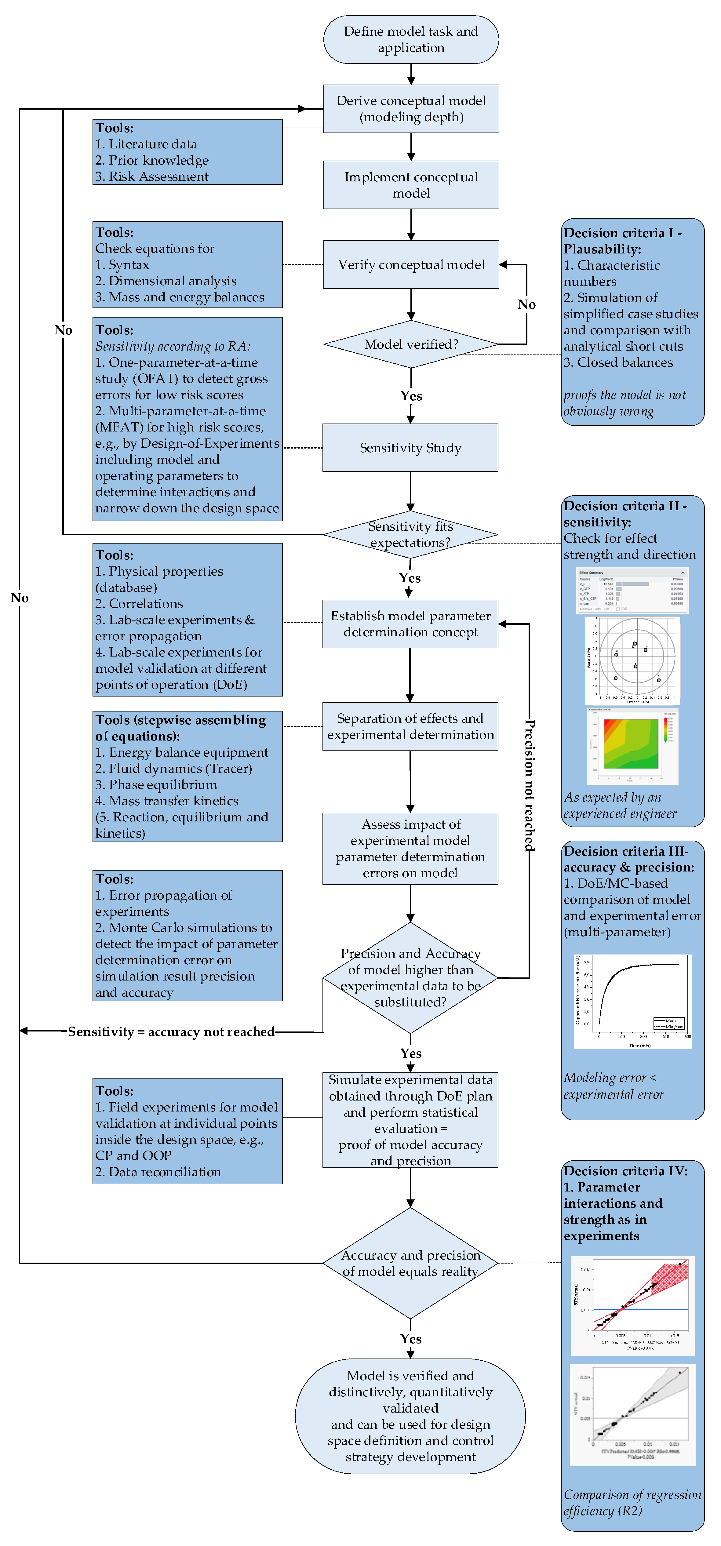
The use of predictive models allows a design space to be defined in a resource-efficient manner and a quantitatively defined and knowledge-based process optimum to be determined. They enable a reduction in experimental effort because they are derived from physico-chemical and thus do not lose their validity when the limits of the design space are exceeded. Thus, process design becomes possible not only on a purely empirical basis, but also leads to a model- and data-based process evaluation. A prerequisite for the possibility of using predictive models is that they can be shown to be at least as accurate and precise as the experiments they are intended to replace [44,48]. The proof can be provided by following the workflow for process development and validation shown in Figure 5 and includes four different decision criteria for each development and validation step [44,49]. After defining the model task and application, the model depth is determined. This is achieved based on existing prior knowledge and the literature. Verification of the model can be achieved by testing the energy and mass balance using simplified case studies. One-parameter-at-a-time studies can be used to infer the sensitivity of the model and determine whether the model behaves as expected. To identify the impact of each parameter, the deviations of the parameters from the center point must be large. By applying DoE principles to create a screening design as a plan for the simulation studies, the sensitivity of the model can be quantified. Unlike the one-parameter-at-a-time studies, the area investigated in the DoE should be within the system boundaries. The quantification of the results can be achieved with the help of statistical evaluations such as partial least squares (PLS) stress diagrams. The final step is to investigate the precision and accuracy of the model at different operating points using, e.g., Monte Carlo simulations. As a rule, the results of the simulation studies are compared with experimental data for final model validation [44,48].

2. Modeling of In Vitro Transcription

Three different reactors are considered in the modeling of in vitro transcription, with balancing taking place in the system boundaries shown in Figure 6.

2.1. In Vitro Transcription and Co-Transcriptional Capping Kinetics

The kinetics of in vitro transcription and the co-transcriptional capping were equal for all operation modes. The equations were adopted from the literature and are based on Michaelis–Menten-type kinetics with consideration of byproduct inhibition. The maximum reaction rate was a function of the turnover rate (${\mathrm{k}}_{\mathrm{eff}}$) and the enzyme concentration (${\mathrm{c}}_{\mathrm{E}}$).

$$r_{max}=k_{eff}·c_e.$$

(14)

The reaction rate of the in vitro transcription with co-transcriptional capping is given by

$$\begin{gathered} r=\frac{r_{max}}{1+{{\displaystyle \sum }}_{j=1}^N\frac{K_{M,NTP,j}}{c_{NTP,j}}·(1+\frac{c_{PPi}}{K_{I,PPi}}+{{\displaystyle \sum }}_{i=1}^N\frac{c_{NTP,i}}{K_{I,PPi}})+\frac{K_{M,DNA}}{c_{DNA}}·[1+\frac{K_G}{c_{GTP}}·(1+\frac{c_{PPi}}{K_{I,PPi}}+{{\displaystyle \sum }}_{i=1}^{N-1}\frac{c_{NTP,i}}{K_{I,NTP,i}})]}·\frac{c_{cap}}{c_{cap}+K_{M,cap}} \\ ·\frac{c_{mRNA}}{c_{mRNA}+K_{M,mRNA}} \end{gathered}$$

(15)

and describes the influence of the concentrations of the nucleotides (${\mathrm{c}}_{\mathrm{NTP}}$), the pyrophosphate (${\mathrm{c}}_{{\mathrm{PP}}_{\mathrm{i}}}$), the promoter (${\mathrm{c}}_{\mathrm{DNA}}$), and the cap analogue (${\mathrm{c}}_{\mathrm{cap}}$), as well as the mRNA (${\mathrm{c}}_{\mathrm{mRNA}}$) and the inhibition by the nucleoside tri phosphates (${\mathrm{K}}_{\mathrm{I},\mathrm{NTP}}$) and the pyrophosphate (${\mathrm{K}}_{\mathrm{I},{\mathrm{PP}}_{\mathrm{i}}}$). ${\mathrm{K}}_{\mathrm{M},\mathrm{NTP}}$, ${\mathrm{K}}_{\mathrm{M},\mathrm{DNA}}$, ${\mathrm{K}}_{\mathrm{M},\mathrm{cap}}$, and ${\mathrm{K}}_{\mathrm{M},\mathrm{mRNA}}$ are the Monod constants of the nucleotides, the promoter, the cap analogue, and the mRNA, respectively. ${\mathrm{K}}_{\mathrm{G}}$ represents the dissociation constant for initial GTP binding, ${\mathrm{c}}_{GTP}$ is the concentration of guanosine triphosphate. The equation in the square brackets in the denominator of the first fraction describes the initiation process of in vitro transcription, which is characterized by the binding of the promoter to the enzyme. The kinetics of this process are modeled by the binding of the GTP, the inhibition by the pyrophosphate, and the competition of the substrate nucleotides, without GTP.

2.2. Batch and CSTR Production

The production of mRNA in a stirred tank reactor was described by the general mass balance equation for stirred tank reactors. The change in mass over time is equal to the sum of mass flow into and out of the reactor and the mass produced or consumed in a particular reaction, described by r according to the kinetic equations given above.

The changes in product and substrate concentrations over time were calculated by

$$\frac{d{c}_{mRNA}}{dt}=\frac{\left({\dot{V}}_{in}·c_{mRNA,in}-{\dot{V}}_{out}·c_{mRNA}\right)}{V}+r.$$

(16)

$$\frac{d{c}_{NTP,i}}{dt}=\frac{\left({\dot{V}}_{in}·c_{NTP,i,in}-{\dot{V}}_{out}·c_{NTP,i}\right)}{V}-f_i·n_{mRNA}·r$$

(17)

$$\frac{d{c}_{PPi}}{dt}=\frac{\left({\dot{V}}_{in}·c_{PPi,in}-{\dot{V}}_{out}·c_{PPi}\right)}{V}+(n_{mRNA}-1)·r$$

(18)

$$\frac{d{c}_{cap}}{dt}=\frac{\left({\dot{V}}_{in}·c_{cap,in}-{\dot{V}}_{out}·c_{cap}\right)}{V}-r$$

(19)

$$\frac{d{c}_{AdoHcy}}{dt}=\frac{\left({\dot{V}}_{in}·c_{AdoHcy,in}-{\dot{V}}_{out}·c_{AdoHcy}\right)}{V}+r$$

(20)

where f is the relative portion of the base contained in the mRNA, ${\mathrm{n}}_{\mathrm{mRNA}}$ is the transcript length of the mRNA, ${\mathrm{c}}_{\mathrm{AdoHcy}}$ is the S-Adenosyl L-homocysteine concentration, $\dot{\mathrm{V}}$ is the volumetric flowrate either in or out of the reactor, and V is the reaction volume.

The change in volume over time was calculated using a volume balance:

$$\frac{dV}{dt}={\dot{V}}_{in}-{\dot{V}}_{out}.$$

(21)

The process was either simulated in batch mode where incoming and outgoing streams were set to zero, or as a continuously stirred tank reactor (CSTR), where the volumetric flux into and out of the reactor were equal in magnitude and greater than zero.

2.3. Plug Flow Tubular Reactor

The development of fundamental equations for reaction processes and kinetics in continuous flow systems has been reported in the literature as early as 1931 by Benton [52]. Comprehensive analysis of these equations and their dimensional analysis as well as the provision of a boundary condition was performer by Hulburt [53]. The effect of axial dispersion on residence time distribution and concentration profiles of solutes in flow reactors and similar tubular channels was extensively studied and described by Danckwerts in 1953 [54], who derived the well-known Danckwerts boundary conditions, as well as by Taylor [55] and his solution for the axial dispersion coefficient, which was modified by Aris in 1956 [56], also known as the Taylor–Aris solution. Bischoff and Levenspiel showed the interrelationship of the different models for longitudinal and radial dispersion present at that time in 1962 [57,58]. Major contributions to the understanding of laminar dispersion were made by Wissler [59], Ananthakrishnan et al. [60], and Chee-Gen and Ziegler [61], who investigated the validity of Taylor and Aris’s solution for different flow regimes. Wissler also provided an alternative inlet boundary condition, in which the limit of large Peclet numbers provides better results for the semi-infinite reactor when compared to the Wehner–Wilhelm equation [62]. Among the first works, Trivedi and Vasudeva [63] extensively studied the reduction in dispersion by different vessel geometries, such as coiled helices, when compared to the straight tube, which was the model geometry primarily investigated up to this point in time. In this context, Saxena and Nigam [64] demonstrated the effect of coiled configurations for flow inversion on the residence time distribution and provided a correlation including a design parameter, which interconnects dispersion and the number of bends. Westerterp et al. [65,66,67] compared the standard dispersion model with other model solutions and introduced the so-called wave model, based on hyperbolic equations opposed to parabolic as in the dispersion model, for the description of longitudinal dispersion in tubular reactors. Since then, many studies have been published for chemical as well as pharmaceutical reaction processes; however, the axial dispersed plug flow model as well as the boundary conditions for the closed–closed vessel as described by Danckwerts have remained the model approach of choice due to their effective prediction capabilities of non-ideal flow reactors.

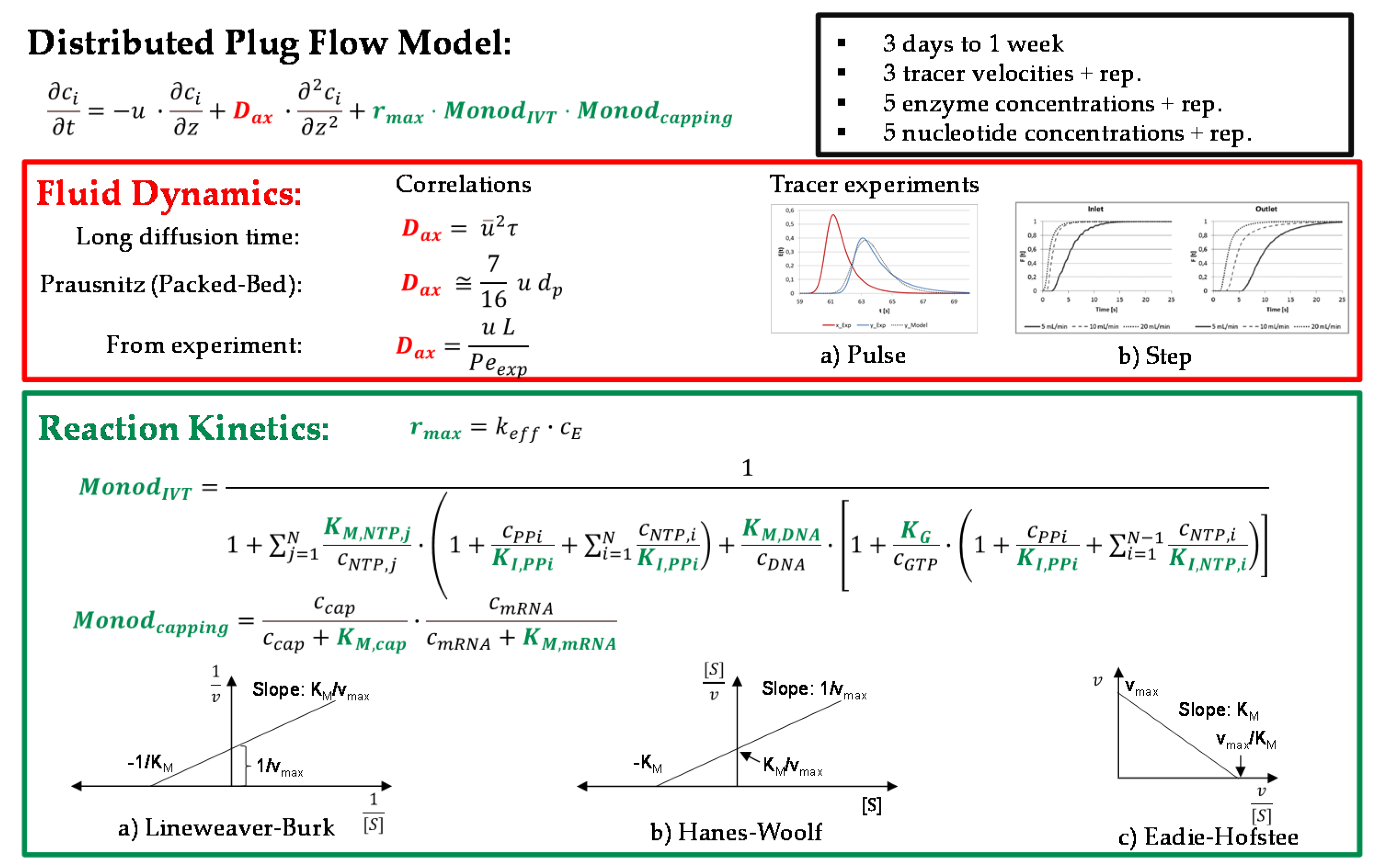
The change in concentration over time was modeled by an axial dispersion model. In this model, the overall concentration change is equal to the sum of the change in concentration over the reactor length resulting from convection by the fluid velocity $u,$ concentration change by dispersion in analogy to Fick’s law, where the parameter D_ax describes the extent of back mixing and the concentration change due to reaction, $r$, according to the kinetic equations given above

$$\frac{\partial c_i}{\partial t}=-u ·\frac{\partial c_i}{\partial z}+D_{ax} ·\frac{{\partial }^2{c}_i}{\partial z^2}+r.$$

(22)

The corresponding differential equations can be solved by the implementation of two boundary conditions, which are shown in Equations (23) and (24).

$$\frac{\partial c\left(z=L\right)}{\partial z}=0$$

(23)

$$D_{ax}·\frac{\partial c\left(z=0\right)}{\partial z}=u· \left(c\left(z=0\right) - c_{in}\right)$$

(24)

Table 2. Reference conditions for in vitro transcription.

Process Variable	Value	Unit
Transcript length	4079	Bases
RNA polymerase concentration	1 × 10−3	mM
Nucleotide concentration	5	mM
Cap analog concentration	9.1	mM
Template concentration	2 × 10−5	mM
Duration	9	h
Throughput 1	0.19	L/h
L/D 2	2500	-
Temperature	37	°C

¹ For CSTR and PFR. ² of the PFR.

shows the reference conditions for the in vitro transcriptions of all reactor types. The values were adapted from the literature [3,9,17,68].

3. Model Parameter Determination

Figure 7 shows a workflow for the model parameter determination. The fluid dynamics (red) of the system are characterized by the axial dispersion coefficient. This can be determined with the help of tracer experiments by inducing the tracer either as a pulse or as a step [69]. Alternatively, correlations of the axial dispersion coefficient can be used. Examples are the correlations for a long diffusion time, for experimentally determined Peclet numbers, and for a packed bed according to Prausnitz [70].

The kinetics of the reactions that take place depend on the maximum reaction rate, the Monod constants of the substrates and the promoter, which is located on the template DNA. It is also influenced by the inhibition constants of the substrates and the products. These parameters can be determined by evaluating the Lineweaver–Burk [71,72], the Hanes–Woolf [73], or the Eadie–Hofstee diagrams [74].

Alternatively, if available, reaction parameters can be derived from the literature or enzymatic databases [75].

4. Model Validation

4.1. Sensitivity Analysis

The model validation starts with the model verification. Here, it is checked if the syntax is correct, and a dimension analysis is performed. All mass balances must be closed, and results of test simulations must correspond to the expert expectations. Characteristic numbers describing fluid dynamics, e.g., Reynolds or Péclet, and mass transfer kinetics, e.g., Schmidt, should be used to ensure the validity of the model. Model sensitivity should first be investigated with respect to the influence of the individual model parameters. This must be performed at least for the univariate parameters identified in the risk assessment. It is better to perform this for all model parameters. The results are discussed in Section 4.1.1.

The model parameters to be investigated in the risk assessment as multivariate are quantified with tools of statistical experimental design with respect to their sensitivity (effect strength and direction), and their influence on the space–time yield by the multidimensional design space is determined. The results are presented in Section 4.1.2. Finally, it must be ensured that the prediction range due to the error in the model parameter determination, determined by Monte Carlo simulation, is smaller than the experimental error. This is discussed in Section 4.2.

4.1.1. One-Factor-at-a-Time

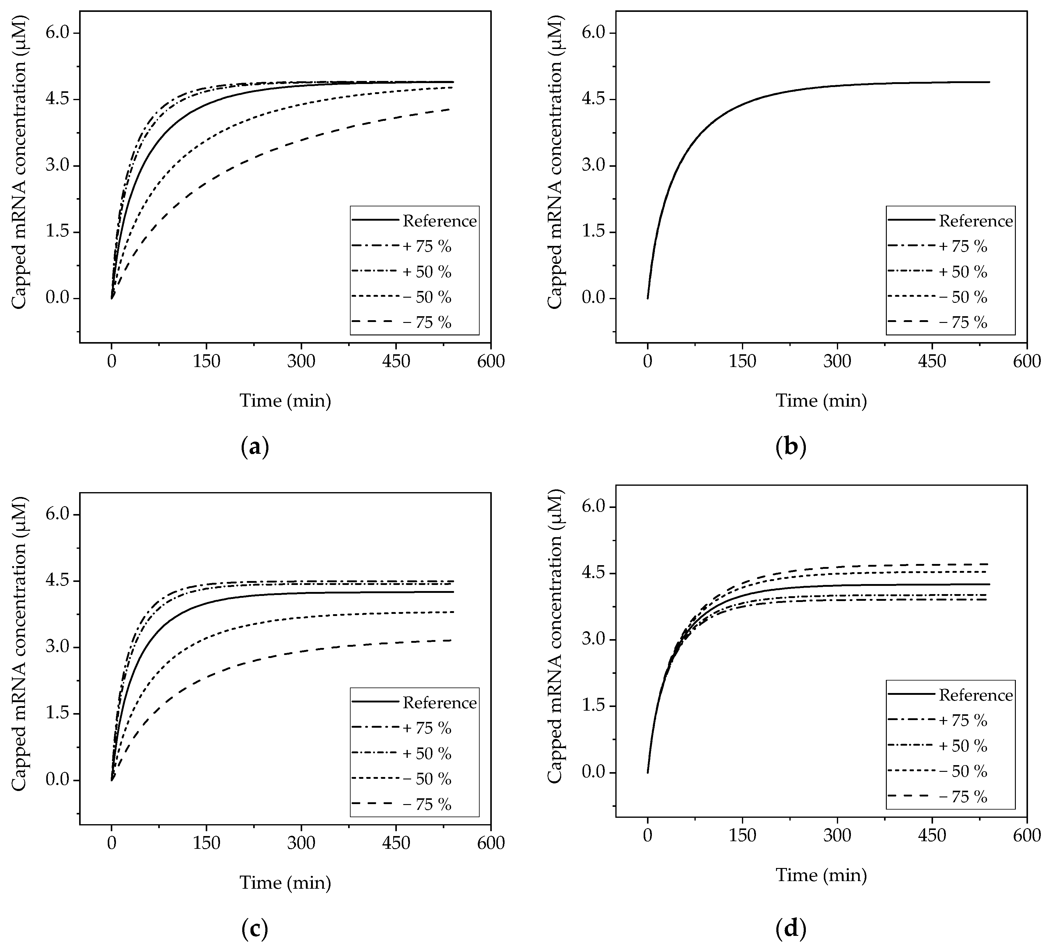
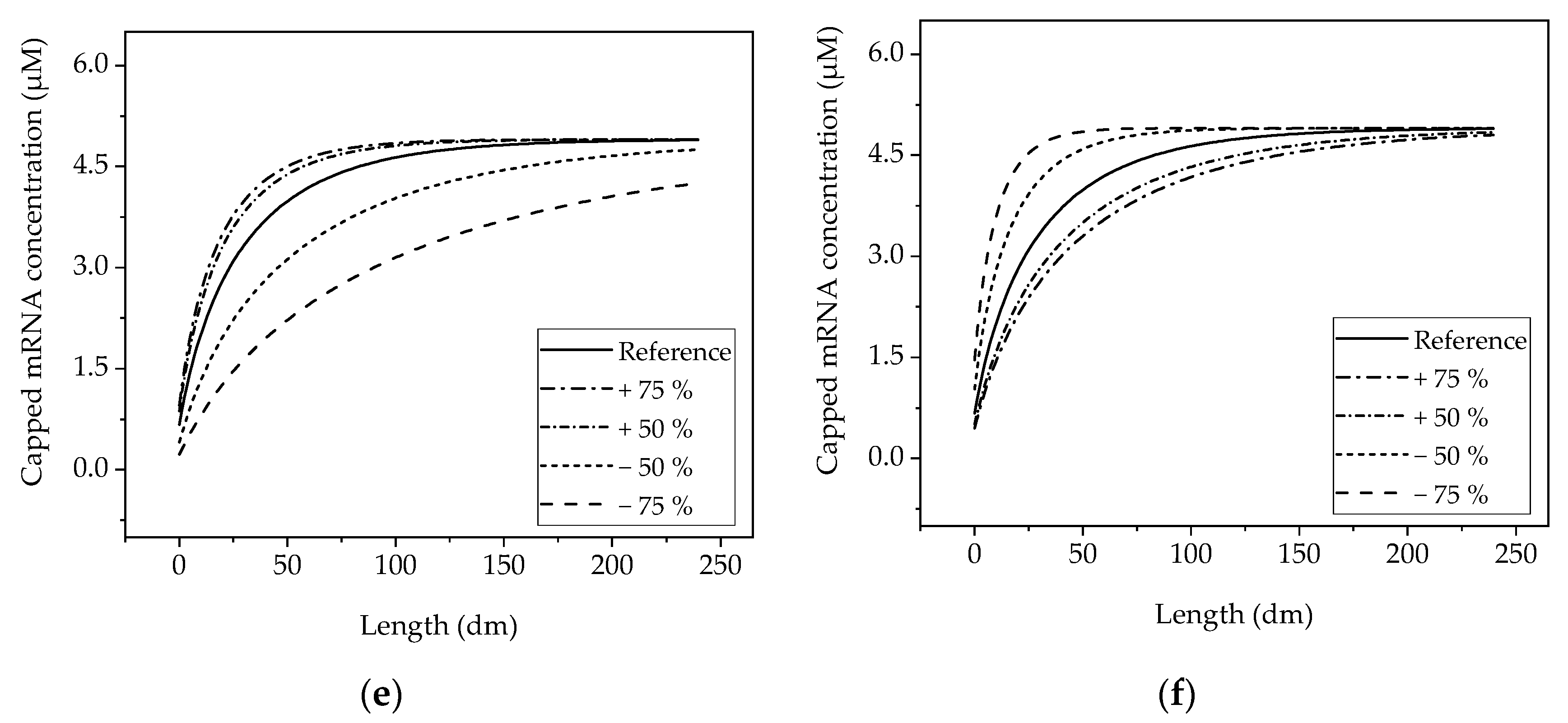
The obtained sensitivities by varying one factor at a time can be seen in Figure 8 for selected factors. Since the selected reference operating point already achieves complete conversion within the reaction time investigated, the same final concentration as in the reference condition is achieved when the enzyme concentration is increased. However, as expected, increasing the enzyme concentration has a positive effect on the kinetics, so that the final capped mRNA concentration is reached earlier (Figure 8a). The Monod constant of the cap analogue does not show a strong influence on the kinetics of production of the capped mRNA (Figure 8b).

When the concentration is decreased, the reaction slows down so that less capped mRNA is obtained at the end of the time period studied than in the reference condition. Due to the similar mean reaction time in the batch and PFR scenarios, the concentration profiles obtained correspond to each other with respect to the ordinate considered.

In the CSTR (Figure 8c,d), the same effects are observed, but the concentration profile does not quantitatively match that of batch and PFR (Figure 8e,f) due to the constant dilution by the input stream. This also causes a different final concentration.

In contrast to the strong positive effect due to the change in enzyme concentration, a change in the Monod constant of mRNA does not cause a deviation from the reference concentration profile greater than five percent at any time.

The effect of throughput Q (omitted in the batch scenario) shows the expected negative influence on the final concentration. This is due to the reduction in the residence time and thus the available reaction time. This observation based on the parameters fully examined here is representative of the fact that there is no obvious error in the implementation, such that part of the decision criterion for sensitivity is met.

4.1.2. Multiple Factors at a Time

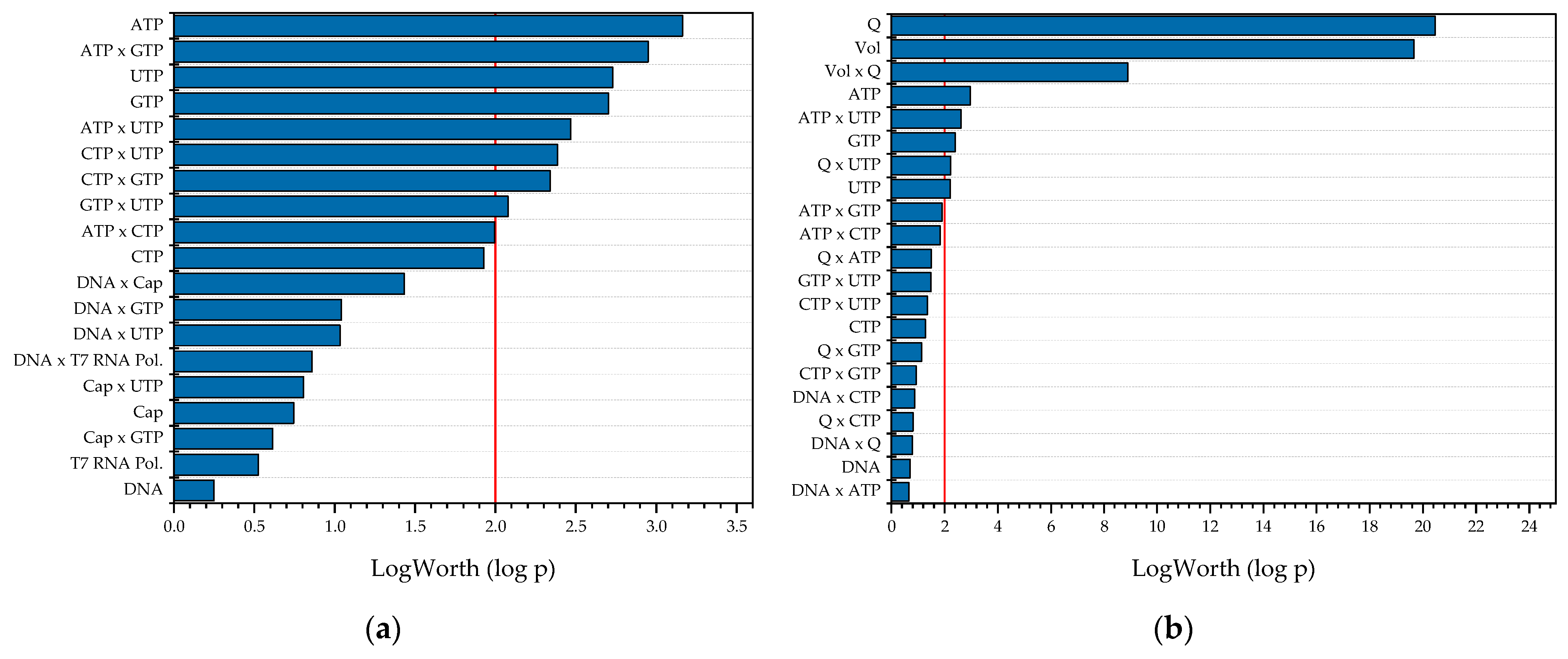
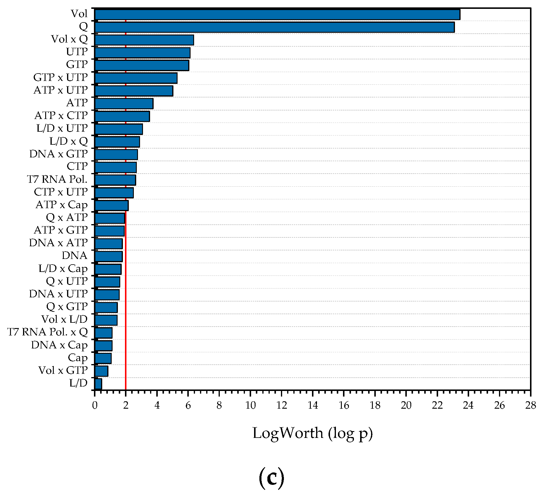
Multiple-factors-at-a-time (MFAT) studies are performed to quantify the effects of the process variables on space–time yield and also to map possible interactions between the parameters. The parameters considered have a high risk score. The MFAT studies were conducted on a DoE basis. The DoE was a two-stage partial factorial custom design to allow for two-way interactions. Depending on the process model investigated, 8, 9, and 11 factors were examined for batch, CSTR, and PFR, respectively.

Figure 9 shows the results from the MFAT studies. As expected, the most significant effects on the space–time yield for both CSTR and PFR are the reactor volume, since as the volume decreases, the space efficiency increases, as does the volume flow rate, whereas as the volume flow rate increases, the time efficiency increases. In addition, the nucleotide concentrations as well as their interactions affect the target size. This is also the case with the batch reactor. In contrast to the other two reactors, the enzyme concentration is the most significant effect here, whereas it becomes insignificant in the CSTR and PFR, due to the linear dependence of the space–time yield on the throughput.

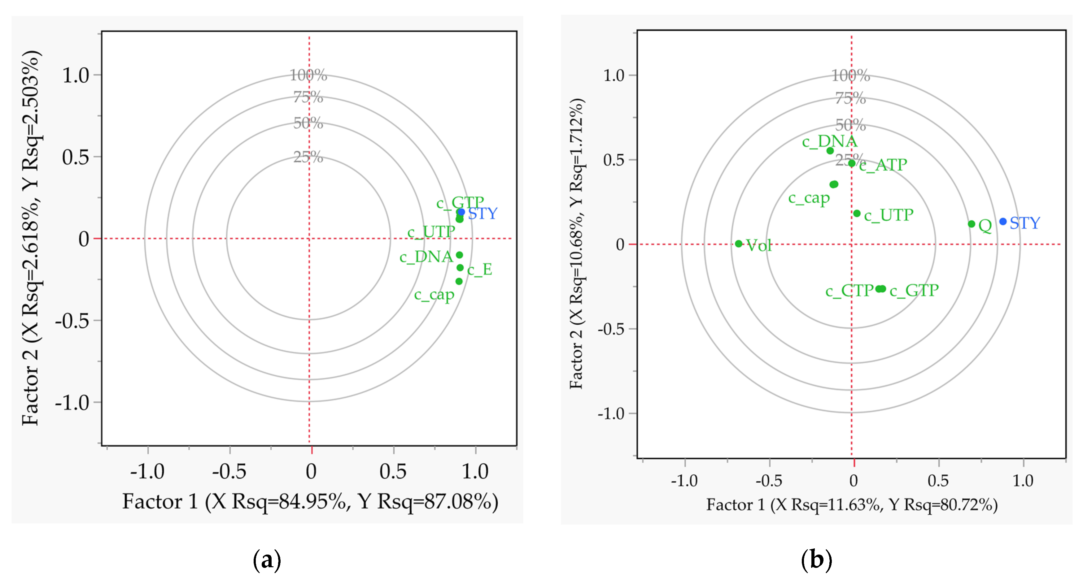
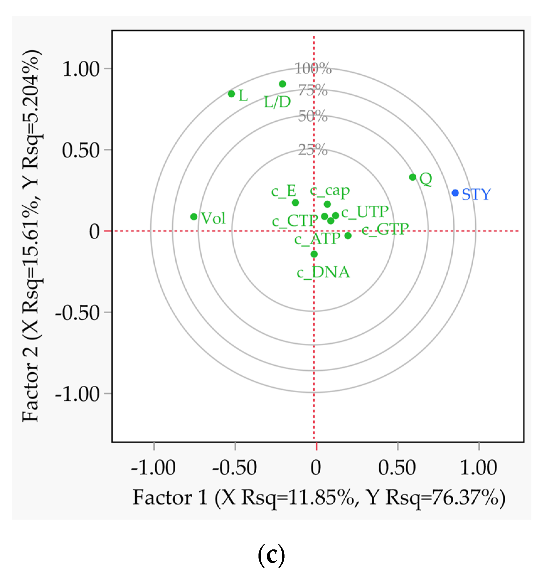
The partial least squares (PLS) loading plots, shown in Figure 10, make it possible to recognise and understand linear dependencies of the covariance at a glance. In the batch reaction all factors are positively correlated with STY (Figure 10a). In the case of the CSTR, the volume is negatively correlated with STY, since higher values decrease the space efficiency of the process (Figure 10b). For example, the space-time yield (STY) takes on high values when the length-to-diameter ratio is high (Figure 10c) and the volume is low at the same time. A linear dependency is only present for volume, while length and geometry ratio can be considered independent variables due to their orthogonal position to STY.

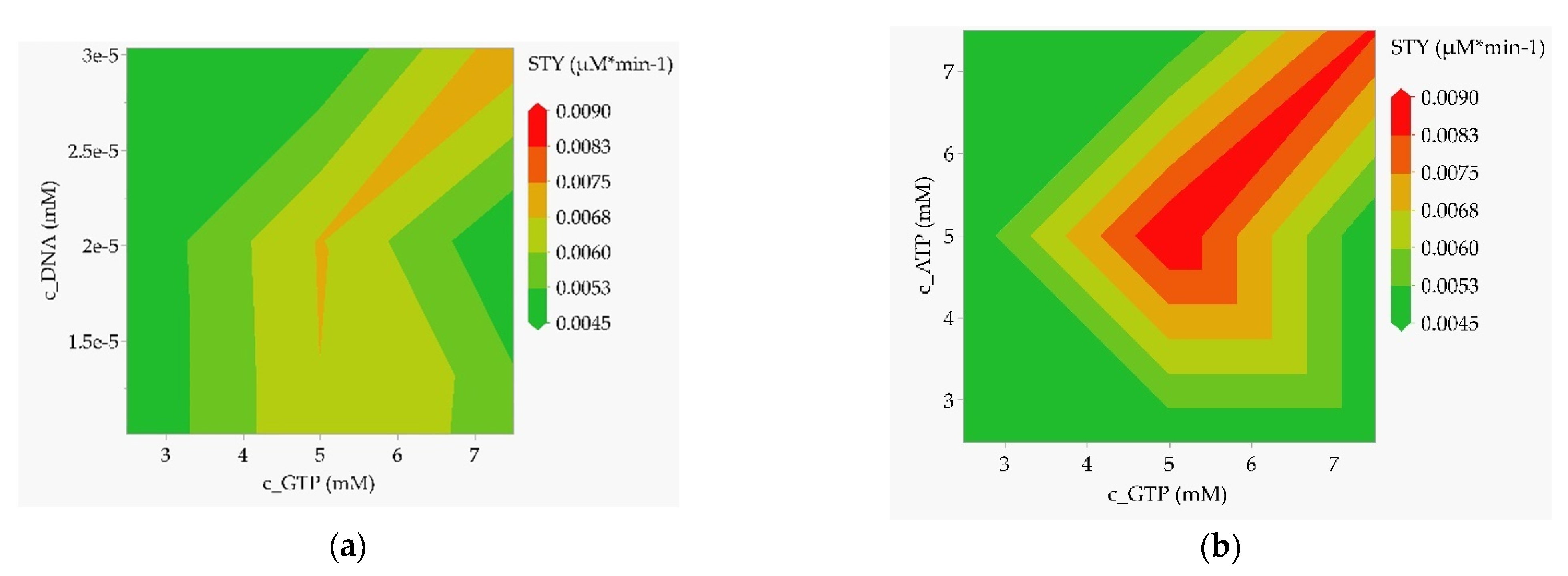
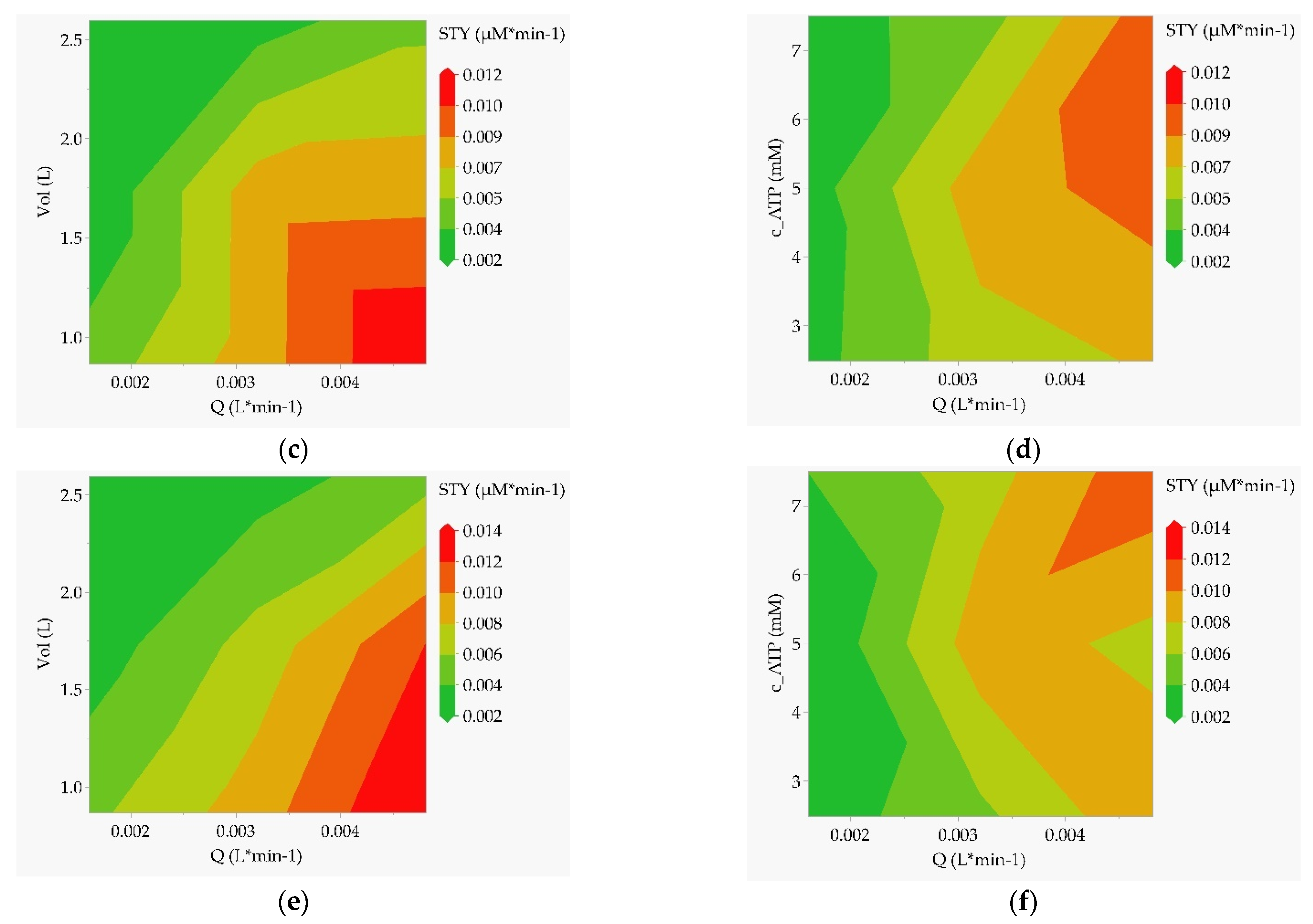
Finally, a preliminary design space can already be narrowed down by plotting the STY over the most important influencing factors resulting from the effects analysis (see Figure 11). In the case of the batch reactor (Figure 11a,b), the optimum can be located at high template DNA and nucleotide concentrations. Within the “green” to “dark green” regions, the STY drops to below 50% of the predicted optimum.

In the case of the CSTR (Figure 11c,d) and PFR (Figure 11e,f), the parameters that emerge as most significant from the effects analysis are volume and throughput. The optimum is found at low volume (lower bound here) and high throughput (upper bound here). A lower acceptable operating range can again be clearly defined via the contour limits. The nucleotide concentration must also be increased with increasing throughput to achieve the highest possible STY.

Thus, from the MFAT studies, the interaction effects as well as a confined design space emerged with clear and quantitative sensitivities, thus achieving the second validation criterion.

4.2. Accuracy and Precision

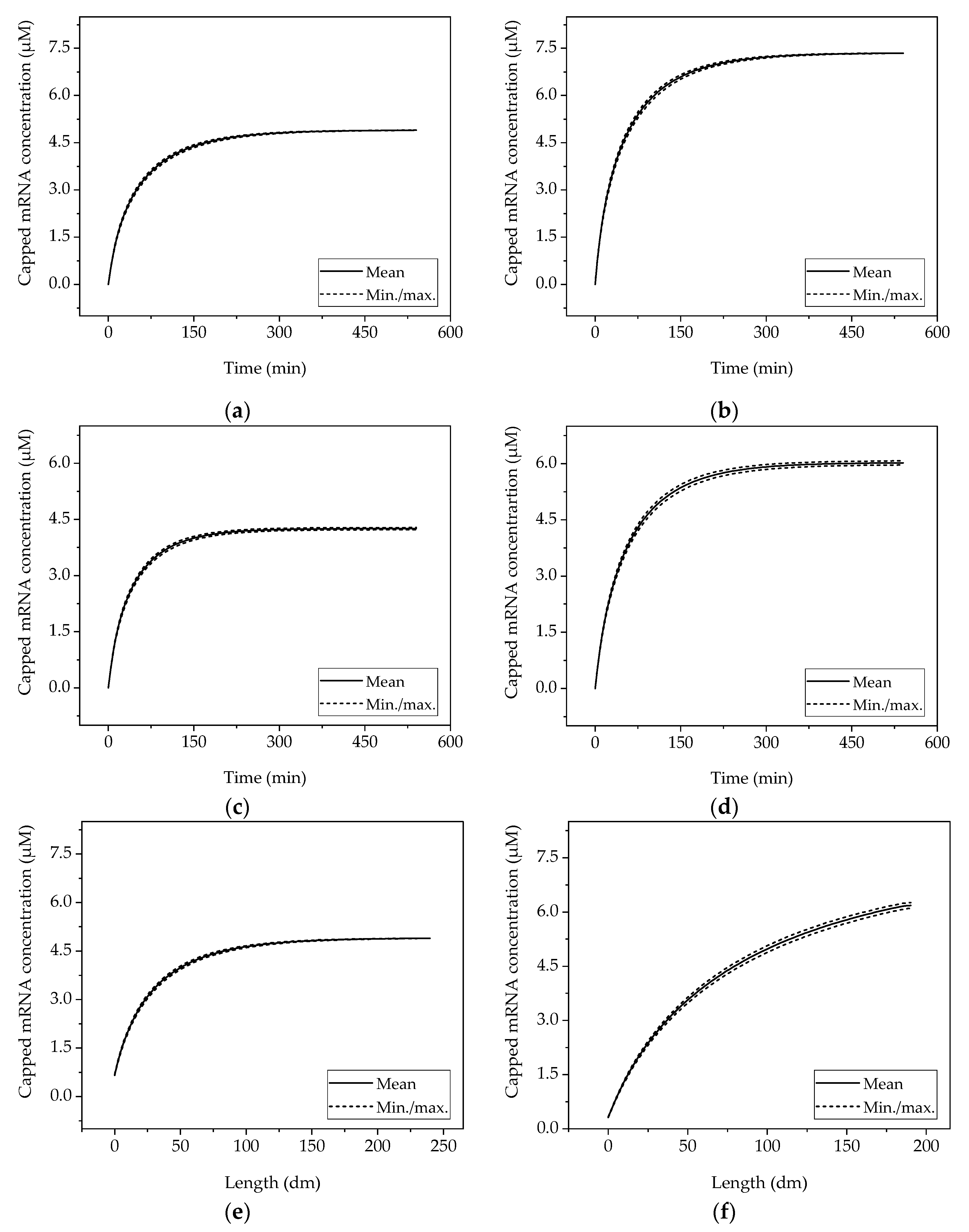
Determination of model precision and accuracy is investigated here via Monte Carlo studies. In this paper, the authors present only the results on precision. The design space described in the MFAT study is simulated here at the center point and the optimum predicted from statistical regression. The reference STY (CP) is 50.0% higher for the batch reactor at the optimum operating point (OOP), 41.6% higher for the CSTR, and 48.4% higher for the PFR. Likewise, the final mRNA concentration increases from 4.9 µM to 7.3 µM (batch), from 4.3 µM to 6.0 µM (CSTR), and from 4.9 µM to 7.3 µM (PFR) (see Figure 12). Both operating points show a maximum deviation of less than 1% from the mean value for all reactors in the MC simulation.

Typical experimental reproducibilities are around 5%. With 30 simulations performed with a normally distributed, random combination of the assumed model parameter errors of 5%, a t-test confidence interval of 94.97% is obtained with a certainty of 99%. The simulation results deviating by less than 1% can be assumed as sufficiently accurate model predictions. The third criterion is thus fulfilled with regard to precision.

4.3. Comparison of Batch and Continuous Production

Figure 13 shows the comparison of STY for batch reactor, CSTR, and PFR production. The STY is 0.0136 µM/min in the case of a batch campaign. If this is compared to the STY of the CSTR and the PFR at the same production time, the STY of the PFR is at an almost equal level (0.0135 µM/min). However, the STY of the CSTR is only 82% (0.0112 µM/min) of that of the batch reactor due to the dilution effect.

The advantages of continuous production are revealed when the time-dependent STY of the batch reactor is compared with the constant STY of the CSTR and PFR over production campaigns of several days. In the case of a three-day production campaign, the STY of the batch reactor drops to 0.0017 µM/min. In comparison, the continuous reactors show a higher STY by a factor of 66 (CSTR) and by a factor of 79 (PFR). If continuous production is extended to 26 days, the benefits increase to a factor of 57 (CSTR) and 69 (PFR) relative to the batch reactor.

Three-day continuous production is considered technically feasible and can be easily integrated into a downstream process on a paragraph-by-paragraph basis. A 26-day continuous production, although allowing the greatest efficiency gains to be achieved, is more technically challenging as it requires continuous reprocessing. Pioneering work on this is already known for other stock systems [76]. A key technology to enable robust continuous production over such a long period is the digital twin as the basis of a sophisticated control strategy.

5. Conclusions

Due to the ongoing coronavirus pandemic, the demand for mRNA vaccines remains very high and currently exceeds production capacity. In order to increase the productivity of existing facilities, the conversion from the currently operated batch to continuous mRNA production is a promising option.

In this article, a distinct and quantitative validated process model for continuous mRNA production in a tubular reactor was developed and compared to batch and continuous mRNA production in an STR, applying the model validation workflow presented by Sixt et al. [44].

The validated models describe mRNA formation and substrate consumption by a Michaelis–Menten-type kinetic that was specifically derived for mRNA transcription. The model includes the fluid dynamics of the PFR and can thus be used independently of the scale of the reactor, as long as characteristic numbers such as Reynolds, Péclet, Sherwood, and Schmidt remain constant, and the fluid dynamics have been determined experimentally at the respective scale.

The model is thus also suitable for scale up, e.g., from laboratory to pilot or production scale. For a process model to be applicable, it must also be accurate and precise.

• Model precision is defined by the combination of model depth and the influence of experimental errors in model parameter determination on model prediction.
• If the process model has an accuracy comparable to the accuracy of replicates of experiments, including errors from analytical procedures, it is considered accurate and is thus capable of replacing experiments.

In this study, model accuracy was determined using Monte Carlo simulations and was 99.7% for the PFR. For the batch and the CSTR, the accuracies were 99.95% and 99.1%, respectively, for a variation in the model parameters of 5%.

All three models are thus accurate and can be used as digital twins for batch and continuous mRNA production.

Considering a production time frame of 26 days, the improvements in the space–time yield were determined to be higher by almost a factor of 70 for a tubular reactor compared to a batchwise in vitro transcription.

The next research steps will focus on further experimental validation of the models at the lab scale to test the robustness of the models when applied as digital twins in combination with existing PAT strategies [16,48,49,76,77,78], for advanced process control towards autonomous operation manufacturing concepts.

References

- Linares-Fernández, S.; Lacroix, C.; Exposito, J.-Y.; Verrier, B. Tailoring mRNA Vaccine to Balance Innate/Adaptive Immune Response. Trends Mol. Med. 2020, 26, 311–323. [Google Scholar] [CrossRef] [PubMed]
- Huang, L.; Zhang, L.; Li, W.; Li, S.; Wen, J.; Li, H.; Liu, Z. Advances in Development of mRNA-Based Therapeutics. Curr. Top. Microbiol. Immunol. 2020. [Google Scholar] [CrossRef]
- Sahin, U.; Muik, A.; Vogler, I.; Derhovanessian, E.; Kranz, L.M.; Vormehr, M.; Quandt, J.; Bidmon, N.; Ulges, A.; Baum, A.; et al. BNT162b2 vaccine induces neutralizing antibodies and poly-specific T cells in humans. Nature 2021, 595, 572–577. [Google Scholar] [CrossRef] [PubMed]
- Liu, M.A. A Comparison of Plasmid DNA and mRNA as Vaccine Technologies. Vaccines 2019, 7, 37. [Google Scholar] [CrossRef] [PubMed] [Green Version]
- Sahin, U.; Karikó, K.; Türeci, Ö. mRNA-based therapeutics—Developing a new class of drugs. Nat. Rev. Drug Discov. 2014, 13, 759–780. [Google Scholar] [CrossRef] [PubMed]
- Meo, S.A.; Bukhari, I.A.; Akram, J.; Meo, A.S.; Klonoff, D.C. COVID-19 vaccines: Comparison of biological, pharmacological characteristics and adverse effects of Pfizer/BioNTech and Moderna Vaccines. Eur. Rev. Med. Pharmacol. Sci. 2021, 25, 1663–1669. [Google Scholar]
- Tanne, J.H. COVID-19: FDA approves Pfizer-BioNTech vaccine in record time. BMJ 2021, 374, n2096. [Google Scholar] [CrossRef]
- Schlake, T.; Thess, A.; Fotin-Mleczek, M.; Kallen, K.-J. Developing mRNA-vaccine technologies. RNA Biol. 2012, 9, 1319–1330. [Google Scholar] [CrossRef] [PubMed] [Green Version]
- Kis, Z.; Kontoravdi, C.; Shattock, R.; Shah, N. Resources, Production Scales and Time Required for Producing RNA Vaccines for the Global Pandemic Demand. Vaccines 2020, 9, 3. [Google Scholar] [CrossRef] [PubMed]
- Mihokovic, N. Continuous Manufacturing-EMA Perspective and Experience. 2017. Available online: https://dc.engconfintl.org/biomanufact_iii/69/ (accessed on 3 September 2021).
- Chatterjee, S. FDA Perspective on Continuous Manufacturing. IFPAC Annual Meeting, Baltimore, MD. 2012. Available online: https://gmpua.com/Process/ContinuousManufacturing/ContinuousManufacturing.pdf (accessed on 10 September 2021).
- Woodcock, J. Modernizing pharmaceutical manufacturing–continuous manufacturing as a key enabler. In Proceedings of the International Symposium on Continuous Manufacturing of Pharmaceuticals, Cambridge, MA, USA, 20 May 2014. [Google Scholar]
- Beg, S.; Hasnain, M.S.; Rahman, M.; Swain, S. Introduction to Quality by Design (QbD): Fundamentals, Principles, and Applications. Pharmaceutical Quality by Design; Elsevier: Amsterdam, The Netherlands, 2019; pp. 1–17. ISBN 9780128157992. [Google Scholar]
- Yu, L.X. Pharmaceutical quality by design: Product and process development, understanding, and control. Pharm. Res. 2008, 25, 781–791. [Google Scholar] [CrossRef]
- Chen, Y.; Yang, O.; Sampat, C.; Bhalode, P.; Ramachandran, R.; Ierapetritou, M. Digital Twins in Pharmaceutical and Biopharmaceutical Manufacturing: A Literature Review. Processes 2020, 8, 1088. [Google Scholar] [CrossRef]
- Schmidt, A.; Helgers, H.; Vetter, F.L.; Juckers, A.; Strube, J. Digital Twin of mRNA-Based SARS-COVID-19 Vaccine Manufacturing towards Autonomous Operation for Improvements in Speed, Scale, Robustness, Flexibility and Real-Time Release Testing. Processes 2021, 9, 748. [Google Scholar] [CrossRef]
- Arnold, S.; Siemann, M.; Scharnweber, K.; Werner, M.; Baumann, S.; Reuss, M. Kinetic modeling and simulation of in vitro transcription by phage T7 RNA polymerase. Biotechnol. Bioeng. 2001, 72, 548–561. [Google Scholar] [CrossRef]
- Geall, A.J.; Mandl, C.W.; Ulmer, J.B. RNA: The new revolution in nucleic acid vaccines. Semin. Immunol. 2013, 25, 152–159. [Google Scholar] [CrossRef]
- Fuchs, A.-L.; Neu, A.; Sprangers, R. A general method for rapid and cost-efficient large-scale production of 5′ capped RNA. RNA 2016, 22, 1454–1466. [Google Scholar] [CrossRef] [Green Version]
- Cunningham, P.R.; Ofengand, J. Use of inorganic pyrophosphatase to improve the yield of in vitro transcription reactions catalyzed by T7 RNA polymerase. Biotechniques 1990, 9, 713–714. [Google Scholar]
- Guajardo, R.; Sousa, R. A model for the mechanism of polymerase translocation. J. Mol. Biol. 1997, 265, 8–19. [Google Scholar] [CrossRef] [PubMed]
- Rosa, S.S.; Prazeres, D.M.F.; Azevedo, A.M.; Marques, M.P.C. mRNA vaccines manufacturing: Challenges and bottlenecks. Vaccine 2021, 39, 2190–2200. [Google Scholar] [CrossRef] [PubMed]
- Higman, M.A.; Christen, L.A.; Niles, E.G. The mRNA (guanine-7-)methyltransferase domain of the vaccinia virus mRNA capping enzyme. Expression in Escherichia coli and structural and kinetic comparison to the intact capping enzyme. J. Biol. Chem. 1994, 269, 14974–14981. [Google Scholar] [CrossRef]
- Tusup, M.; French, L.E.; de Matos, M.; Gatfield, D.; Kundig, T.; Pascolo, S. Design of in vitro Transcribed mRNA Vectors for Research and Therapy. Chimia 2019, 73, 391–394. [Google Scholar] [CrossRef]
- Shuman, S. Capping Enzyme in Eukaryotic mRNA Synthesis; Elsevier: Amsterdam, The Netherlands, 1995; pp. 101–129. ISBN 9780125400503. [Google Scholar]
- Fabrega, C.; Hausmann, S.; Shen, V.; Shuman, S.; Lima, C.D. Structure and Mechanism of mRNA Cap (Guanine-N7) Methyltransferase. Mol. Cell 2004, 13, 77–89. [Google Scholar] [CrossRef]
- Muttach, F.; Muthmann, N.; Rentmeister, A. Synthetic mRNA capping. Beilstein J. Org. Chem. 2017, 13, 2819–2832. [Google Scholar] [CrossRef]
- Samanta, A.; Krause, A.; Jäschke, A. A modified dinucleotide for site-specific RNA-labelling by transcription priming and click chemistry. Chem. Commun. 2014, 50, 1313–1316. [Google Scholar] [CrossRef]
- Pasquinelli, A.E.; Dahlberg, J.E.; Lund, E. Reverse 5′ caps in RNAs made in vitro by phage RNA polymerases. RNA 1995, 1, 957–967. [Google Scholar]
- Peng, Z.-H.; Sharma, V.; Singleton, S.F.; Gershon, P.D. Synthesis and application of a chain-terminating dinucleotide mRNA cap analog. Org. Lett. 2002, 4, 161–164. [Google Scholar] [CrossRef] [PubMed]
- Grudzien, E.; Stepinski, J.; Jankowska-Anyszka, M.; Stolarski, R.; Darzynkiewicz, E.; Rhoads, R.E. Novel cap analogs for in vitro synthesis of mRNAs with high translational efficiency. RNA 2004, 10, 1479–1487. [Google Scholar] [CrossRef] [Green Version]
- Jemielity, J.; Fowler, T.; Zuberek, J.; Stepinski, J.; Lewdorowicz, M.; Niedzwiecka, A.; Stolarski, R.; Darzynkiewicz, E.; Rhoads, R.E. Novel “anti-reverse” cap analogs with superior translational properties. RNA 2003, 9, 1108–1122. [Google Scholar] [CrossRef] [PubMed] [Green Version]
- Kwon, H.; Kim, M.; Seo, Y.; Moon, Y.S.; Lee, H.J.; Lee, K.; Lee, H. Emergence of synthetic mRNA: In vitro synthesis of mRNA and its applications in regenerative medicine. Biomaterials 2018, 156, 172–193. [Google Scholar] [CrossRef]
- Gruber, P.; Marques, M.P.C.; O’Sullivan, B.; Baganz, F.; Wohlgemuth, R.; Szita, N. Conscious coupling: The challenges and opportunities of cascading enzymatic microreactors. Biotechnol. J. 2017, 12, 1700030. [Google Scholar] [CrossRef] [PubMed] [Green Version]
- Matsunami, K.; Ryckaert, A.; Peeters, M.; Badr, S.; Sugiyama, H.; Nopens, I.; de Beer, T. Analysis of the Effects of Process Parameters on Start-Up Operation in Continuous Wet Granulation. Processes 2021, 9, 1502. [Google Scholar] [CrossRef]
- Udugama, I.A.; Lopez, P.C.; Gargalo, C.L.; Li, X.; Bayer, C.; Gernaey, K.V. Digital Twin in biomanufacturing: Challenges and opportunities towards its implementation. Syst. Microbiol. Biomanuf. 2021, 1, 257–274. [Google Scholar] [CrossRef]
- Brunet, R.; Guillén-Gosálbez, G.; Pérez-Correa, J.R.; Caballero, J.A.; Jiménez, L. Hybrid simulation-optimization based approach for the optimal design of single-product biotechnological processes. Comput. Chem. Eng. 2012, 37, 125–135. [Google Scholar] [CrossRef] [Green Version]
- Brunef, R.; Kumar, K.S.; Guillen-Gosalbez, G.; Jimenez, L. Integrating process simulation, multi-objective optimization and LCA for the development of sustainable processes. In 21st European Symposium on Computer Aided Process Engineering; Elsevier: Amsterdam, The Netherlands, 2011; pp. 1271–1275. ISBN 9780444538956. [Google Scholar]
- Del Castillo-Romo, A.Á.; Morales-Rodriguez, R.; Román-Martínez, A. Multi-objective optimization for the biotechnological conversion of lingocellulosic biomass to value-added products. In 26th European Symposium on Computer Aided Process Engineering; Elsevier: Amsterdam, The Netherlands, 2016; pp. 1515–1520. ISBN 9780444634283. [Google Scholar]
- Pérez, A.D.; van der Bruggen, B.; Fontalvo, J. Modeling of a liquid membrane in Taylor flow integrated with lactic acid fermentation. Chem. Eng. Process. Process. Intensif. 2019, 144, 107643. [Google Scholar] [CrossRef]
- Mat Isham, N.K.; Mokhtar, N.; Fazry, S.; Lim, S.J. The development of an alternative fermentation model system for vinegar production. LWT 2019, 100, 322–327. [Google Scholar] [CrossRef]
- Da Costa Basto, R.M.; Casals, M.P.; Mudde, R.F.; van der Wielen, L.A.; Cuellar, M.C. A mechanistic model for oil recovery in a region of high oil droplet concentration from multiphasic fermentations. Chem. Eng. Sci. X 2019, 3, 100033. [Google Scholar] [CrossRef]
- Uhlenbrock, L.; Sixt, M.; Strube, J. Quality-by-Design (QbD) process evaluation for phytopharmaceuticals on the example of 10-deacetylbaccatin III from yew. Resour. Effic. Technol. 2017, 3, 137–143. [Google Scholar] [CrossRef]
- Sixt, M.; Uhlenbrock, L.; Strube, J. Toward a Distinct and Quantitative Validation Method for Predictive Process Modeling—On the Example of Solid-Liquid Extraction Processes of Complex Plant Extracts. Processes 2018, 6, 66. [Google Scholar] [CrossRef] [Green Version]
- Pugh, K. Prior Knowledge in Product Development/Design. Available online: www.ema.europa.eu/documents/presentation/presentation-regulators-perspective-session-2-keith-pugh_en.pdf (accessed on 9 September 2021).
- Yu, L.X.; Amidon, G.; Khan, M.A.; Hoag, S.W.; Polli, J.; Raju, G.K.; Woodcock, J. Understanding pharmaceutical quality by design. AAPS J. 2014, 16, 771–783. [Google Scholar] [CrossRef] [Green Version]
- Alt, N.; Zhang, T.Y.; Motchnik, P.; Taticek, R.; Quarmby, V.; Schlothauer, T.; Beck, H.; Emrich, T.; Harris, R.J. Determination of critical quality attributes for monoclonal antibodies using quality by design principles. Biologicals 2016, 44, 291–305. [Google Scholar] [CrossRef]
- Schmidt, A.; Strube, J. Distinct and Quantitative Validation Method for Predictive Process Modeling with Examples of Liquid-Liquid Extraction Processes of Complex Feed Mixtures. Processes 2019, 7, 298. [Google Scholar] [CrossRef] [Green Version]
- Zobel-Roos, S.; Schmidt, A.; Mestmäcker, F.; Mouellef, M.; Huter, M.; Uhlenbrock, L.; Kornecki, M.; Lohmann, L.; Ditz, R.; Strube, J. Accelerating Biologics Manufacturing by Modeling or: Is Approval under the QbD and PAT Approaches Demanded by Authorities Acceptable without a Digital-Twin? Processes 2019, 7, 94. [Google Scholar] [CrossRef] [Green Version]
- Kornecki, M.; Schmidt, A.; Strube, J. PAT as key-enabling technology for QbD in pharmaceutical manufacturing A conceptual review on upstream and downstream processing. Chim. Oggi Chem. Today 2018, 36, 44–48. [Google Scholar]
- Chmiel, H.; Takors, R.; Weuster-Botz, D. Bioprozesstechnik; Springer: Berlin/Heidelberg, Germany, 2018; ISBN 978-3-662-54041-1. [Google Scholar]
- Benton, A.F. The kinetics of gas reactions at constant pressure. J. Am. Chem. Soc. 1931, 53, 2984–2988. [Google Scholar] [CrossRef]
- Hulburt, H.M. Chemical Processes in Continuous-Flow Systems. Ind. Eng. Chem. 1944, 36, 1012–1017. [Google Scholar] [CrossRef]
- Danckwerts, P.V. Continuous flow systems: Distribution of residence times. Chem. Eng. Sci. 1953, 2, 1–13. [Google Scholar] [CrossRef]
- Taylor, G. Dispersion of soluble matter in solvent flowing slowly through a tube. Proc. R. Soc. Lond. A 1953, 219, 186–203. [Google Scholar] [CrossRef]
- Aris, R. On the dispersion of a solute in a fluid flowing through a tube. Proc. R. Soc. Lond. A 1956, 235, 67–77. [Google Scholar] [CrossRef]
- Bischoff, K.B.; Levenspiel, O. Fluid dispersion-generalization and comparison of mathematical models—I generalization of models. Chem. Eng. Sci. 1962, 17, 245–255. [Google Scholar] [CrossRef]
- Bischoff, K.B.; Levenspiel, O. Fluid dispersion—Generalization and comparison of mathematical models—II comparison of models. Chem. Eng. Sci. 1962, 17, 257–264. [Google Scholar] [CrossRef]
- Wissler, E.H. On the applicability of the Taylor—Aris axial diffusion model to tubular reactor calculations. Chem. Eng. Sci. 1969, 24, 527–539. [Google Scholar] [CrossRef]
- Ananthakrishnan, V.; Gill, W.N.; Barduhn, A.J. Laminar dispersion in capillaries: Part I. Mathematical analysis. AIChE J. 1965, 11, 1063–1072. [Google Scholar] [CrossRef]
- Chee-Gen, W.; Ziegler, E.N. On the axial dispersion approximation for laminar flow reactors. Chem. Eng. Sci. 1970, 25, 723–727. [Google Scholar] [CrossRef]
- Wehner, J.F.; Wilhelm, R.H. Boundary conditions of flow reactor. Chem. Eng. Sci. 1956, 6, 89–93. [Google Scholar] [CrossRef]
- Trivedi, R.N.; Vasudeva, K. Axial dispersion in laminar flow in helical coils. Chem. Eng. Sci. 1975, 30, 317–325. [Google Scholar] [CrossRef]
- Saxena, A.K.; Nigam, K.D.P. Coiled configuration for flow inversion and its effect on residence time distribution. AIChE J. 1984, 30, 363–368. [Google Scholar] [CrossRef]
- Westerterp, K.R.; Dil’man, V.V.; Kronberg, A.E. Wave model for longitudinal dispersion: Development of the model. AIChE J. 1995, 41, 2013–2028. [Google Scholar] [CrossRef]
- Westerterp, K.R.; Dil’man, V.V.; Kronberg, A.E.; Benneker, A.H. Wave model for longitudinal dispersion: Analysis and applications. AIChE J. 1995, 41, 2029–2039. [Google Scholar] [CrossRef]
- Kronberg, A.E.; Benneker, A.H.; Westerterp, K.R. Wave model for longitudinal dispersion: Application to the laminar-flow tubular reactor. AIChE J. 1996, 42, 3133–3145. [Google Scholar] [CrossRef] [Green Version]
- Labarta, I.; Hoffman, S.; Simpkins, A. Manufacturing Strategy for the Production of 200 Million Sterile Doses of an mRNA Vaccine for COVID-19. Available online: https://repository.upenn.edu/cbe_sdr/132/ (accessed on 2 September 2021).
- Wellsandt, T.; Stanisch, B.; Strube, J. Characterization Method for Separation Devices Based on Micro Technology. Chem. Ing. Tech. 2015, 87, 150–158. [Google Scholar] [CrossRef]
- Levenspiel, O.; Bischoff, K.B. Patterns of Flow in Chemical Process Vessels. In Advances in Chemical Engineering; Drew, T.B., Hoopes, J.W., Eds.; Elsevier: Burlington, MA, USA, 1964; pp. 95–198. ISBN 9780120085040. [Google Scholar]
- Ault, A. An introduction to enzyme kinetics. J. Chem. Educ. 1974, 51, 381–386. [Google Scholar] [CrossRef]
- Lineweaver, H.; Burk, D. Fundamentals of enzyme kinetics. J. Am. Chem. Soc. 1934, 56, 658–659. [Google Scholar] [CrossRef]
- Hanes, C.S. Studies on plant amylases: The effect of starch concentration upon the velocity of hydrolysis by the amylase of germinated barley. Biochem. J. 1932, 26, 1406–1421. [Google Scholar] [CrossRef] [PubMed]
- Hofstee, B.H. Non-inverted versus inverted plots in enzyme kinetics. Nature 1959, 184, 1296–1298. [Google Scholar] [CrossRef] [PubMed]
- BRENDA. BRENDA—Braunschweig Enzyme Database. Available online: https://www.brenda-enzymes.org/ (accessed on 8 September 2021).
- Kornecki, M.; Schmidt, A.; Lohmann, L.; Huter, M.; Mestmäcker, F.; Klepzig, L.; Mouellef, M.; Zobel-Roos, S.; Strube, J. Accelerating Biomanufacturing by Modeling of Continuous Bioprocessing—Piloting Case Study of Monoclonal Antibody Manufacturing. Processes 2019, 7, 495. [Google Scholar] [CrossRef] [Green Version]
- Helgers, H.; Schmidt, A.; Lohmann, L.J.; Vetter, F.L.; Juckers, A.; Jensch, C.; Mouellef, M.; Zobel-Roos, S.; Strube, J. Towards Autonomous Operation by Advanced Process Control—Process Analytical Technology for Continuous Biologics Antibody Manufacturing. Processes 2021, 9, 172. [Google Scholar] [CrossRef]
- Zobel-Roos, S.; Schmidt, A.; Uhlenbrock, L.; Ditz, R.; Köster, D.; Strube, J. Digital Twins in Biomanufacturing. Adv. Biochem. Eng. Biotechnol. 2021, 176, 181–262. [Google Scholar] [CrossRef] [PubMed]
Figure 1.
Comparison of the two capping mechanisms. Left: post-transcriptional capping with a two-step enzymatic reaction; right: co-transcriptional capping by adding a cap analog, catalysed by the enzyme used in the in vitro transcription [33].
Figure 2.
Levels of a digital twin, starting from a steady-state model, over a dynamic model, a validated model, and a digital shadow to a model-based control [36].
Figure 3.
Workflow of model validation based on a QbD-oriented approach [43]. In a first step, the QTPPs are defined. Subsequently, the CQAs are defined and a risk assessment of the influence of various process parameters on the CQAs is carried out. The risk assessment results in a design space for the process parameters to be investigated, which can be examined either via experiments or by means of a rigorous process model. Based on the results, a control strategy is defined, which can be continuously compared online via PAT with the actual state of the system. Strict implementation of this strategy allows continuous process optimization.
Figure 4.
Ishikawa diagram and corresponding failure mode effect analysis (FMEA). Visualization of influencing variables and effects is a key step in risk assessment in the context of quality-by-design-based process development.
Figure 5.
Decision tree for a process model validation according to Sixt et al. The application allows a quantitative evaluation of the model quality based on mechanistic and statistical decision criteria. A rigorous execution of the procedure leads to a distinctively and quantitatively validated rigorous process model. Solid lines describe the process of a decision, dashed lines show the affiliation of the decision criteria to the respective decision points.
Figure 6.
System boundaries of (a) batch reactor, (b) CSTR, and (c) tubular reactor [51].
Figure 7.
Modeling and parameter determination scheme for in vitro transcription.
Figure 8.
Sensitivity of the models obtained by one-parameter-at-a-time studies. (a) Batch reactor, variation in the T7 RNA polymerase concentration; (b) batch reactor, variation in the Monod constant of the mRNA (lines are overlapping); (c) CSTR, variation in the T7 RNA polymerase concentration; (d) CSTR, variation in the flow rate; (e) tubular reactor, variation in the T7 RNA polymerase concentration; (f) tubular reactor, variation in the flow rate.
Figure 9.
Summary of all relevant effects as a result of the DoE-based multiple-factors-at-a-time sensitivity study with space–time yield (STY) as the target value. (a) Batch reactor; (b) CSTR; (c) tubular reactor.
Figure 10.
Partial least squares analysis correlation loading plots of all relevant effects as a result of the multiple-factors-at-a-time (DoE) sensitivity study with STY as the target value. (a) Batch reactor; (b) CSTR; (c) tubular reactor.
Figure 11.
Contour plots as a result of the multiple-factors-at-a-time (DoE) sensitivity study with STY as the target value. (a) Batch reactor, template DNA concentration over GTP concentration; (b) batch reactor, ATP concentration over GTP concentration; (c) CSTR, reactor volume over the flow rate; (d) CSTR, ATP concentration over the flow rate; (e) tubular reactor, reactor volume over the flow rate; (f) tubular reactor, ATP concentration over the flow rate.
Figure 12.
Deviation of the models obtained by the random variation of process variables with a standard deviation of +/− 5% in Monte Carlo simulations. The left column shows the center point, the right column shows the optimal operating point (derived from DoE) for (a,b) batch reactor, (c,d) CSTR, and (e,f) tubular reactor.
Figure 13.
Comparison of STY (space–time yield) for batch reactor, CSTR (continuous stirred tank reactor), and PFR (plug flow reactor).