Random Forest Regression-Based Machine Learning Model for Accurate Estimation of Fluid Flow in Curved Pipes

Abstract

In industrial piping systems, turbomachinery, heat exchangers etc., pipe bends are essential components. Computational fluid dynamics (CFD), which is frequently used to analyse the flow behaviour in such systems, provides extremely precise estimates but is computationally expensive. As a result, a computationally efficient method is developed in this paper by leveraging machine learning for such computationally expensive CFD problems. Random forest regression (RFR) is used as the machine learning algorithm in this work. Four different fluid flow characteristics (i.e., axial velocity, x-velocity, y-velocity and z-velocity) are studied in this work. The accuracy of the RFR models is assessed by using a number of statistical metrics such as mean-absolute error (MAE), mean-squared-error (MSE), root-mean-squared-error (RMSE), maximum error (Max.Error) and median error (Med.Error) etc. It is observed that the RFR models can produce considerable cost reductions in computing by surrogating the CFD model. Minor loss in estimation accuracy as compared to the CFD models is observed. While the magnitude of intricate flow characteristics such as the additional vortices are correctly predicted, some error in their location is observed.

1. Introduction

Bent pipes and elbows are used in many engineering systems, including water supply systems, oil and gas piping systems, automobile engines, power generation plants, turbo machinery, and heat exchangers. Such flows have a complex character and are usually turbulent. As a result, numerous experimental and computational studies in bend pipes and ducts of several cross-sections have been conducted in response to the growing practical interest in understanding the physical principles driving turbulent flows across pipe bends and elbows. When compared to straight pipes, the main feature of curved pipes is the presence of a secondary motion consisting of a pair of symmetric, counter-rotating vortices. This Prandtl first kind secondary motion increases heat transfer and mixing, for example, effects that are used in many industrial applications, such as nuclear reactor cooling systems, and food processing [1,2,3].

Although curved pipe flows have been studied since the late 19th century (see a detailed description including historical aspects [4]), many questions remain unanswered. Several experiments on turbulent flow have been carried out in curved pipes [5,6,7,8,9,10,11], to name just a few. Measurements of turbulent flow through U-bends with circular and rectangular sections have been reported by Sudo et al. [6]. Helically coiled pipe research has also mostly focused on monitoring pressure or temperature data and determining flow parameters. The flow’s curvature and torsion effects during the laminar to turbulent transition were studied by Cioncolini and Santini [12] and Hayamizu et al. [13]. Due to their sophisticated and resource-intensive nature for completing tests, numerical models of flow in bent pipes have only lately begun to evolve in parallel with the advent of expanding computer resources. Tanaka et al. [14] calculated FVM estimations of water flow in pipe bends for various values of Re and bend curvature using the Large Eddy Simulation (LES) turbulence model. The references [15,16] include a database for LES and Direct Numerical Simulations (DNS) on pipe bend flows. Kim et al. [17] used the FVM-based OpenFOAM software to do numerical simulations of Sudo et al.’s [5] tests and a comparison study to see which turbulence model better matched the experimental results. Rohrig et al. [18] used the OpenFOAM solver to describe turbulent flow in a 90-degree pipe curve. They looked at the wall-resolved LES and various RANS models with Re ranging from 1.4103 to 3.4103 in terms of computing performance. They matched their results to Kalpakli and Orlu’s [9] experimental data to establish the superiority of LES over frequently used RANS techniques, although at a much greater computing cost.

Averaged flow field and measurements of turbulence in curved pipes have primarily been carried out at intermediate Reynolds numbers, Re = (4 to 8) × 104, in recent decades ([5,6,7,11]). Quite the reverse, there are few investigations on pipe bend flow above Re = 4 × 105, when flow properties are expected to be independent of the Reynolds number [17,19]. Recently, Dutta conducted a series of numerical research on pipe bend flow at high Reynolds numbers for different curvature ratios and also concluded the same [20,21,22,23,24,25,26,27]. These experiments were conducted on bends with various bend curvature ratios ranging from Rc/D = 1 to 5 and the Reynolds numbers rang is Re = (1 × 10⁵ to 10 × 10⁵). The findings of previous research are commonly used to power plant pipelines, which frequently utilise pipe bends with a curvature ratio of 1.0 to 1.5. Due to a lack of experimental data, it is currently difficult to offer an explanation for the impact of the bend curvature ratio on the turbulent flow-field and turbulence structure in a pipe bend. In the absence of experimental data, computational fluid dynamics (CFD) models are frequently used, which offer a highly accurate prediction of flow properties in general. However, due to their computational expense, CFD models are not suitable for large-scale deployment. To address this issue, many researchers in technical issues, particularly turbulent flow in curved sections, have used soft-computing techniques in the recent decade.

Artificial neural network (ANN) is one of the most widely used metamodeling method for accurately surrogating complex CFD models for fluid flow problems. In case of large-eddy simulation, Gamahara and Hattori [28] employed ANN to create a subgrid model. To estimate the velocity of fluid flowing through a steep 90° curve, Gholami et al. [29] used ANN with decision trees (DT). Rahimi et al. [30] used ANN to investigate the flow characteristics in serpentine microchannels. Srinivasan et al. [31] evaluated the effectiveness of ANN in recreating reduced-order models in turbulent flows in a recent paper. Ganesh et al. [32] have developed genetic programming (GP)-based metamodels to properly measure fluid flow velocity in 90° pipe bends. Narayanan et al. [33] created the PSO adjusted support vector machine (SVM) model to investigate the turbulent flow field at the elbow. In order to better understand the influence of various parameters on turbulent fluid behaviour at the elbow, they utilised the SVM metamodel to perform a parameter enquiry on the CFD simulation dataset.

Based on the foregoing explanation, it is clear that utilising soft computing to forecast turbulent flow characteristics in pipe bends will considerably reduce the computation time than CFD, but it would be a great challenge in computing a highly nonlinear fluid flow problem accurately. To address this, an ensemble machine learning algorithm called Random Forest Regression (RFR) is used a surrogate to the expensive CFD model. However, RFR model must be accurately trained initially on suitable training data that may be generated through the CFD process. The rest of the manuscript is arranged in the following way—Section 2 introduces the problem tackled in the paper.

2. Methodology

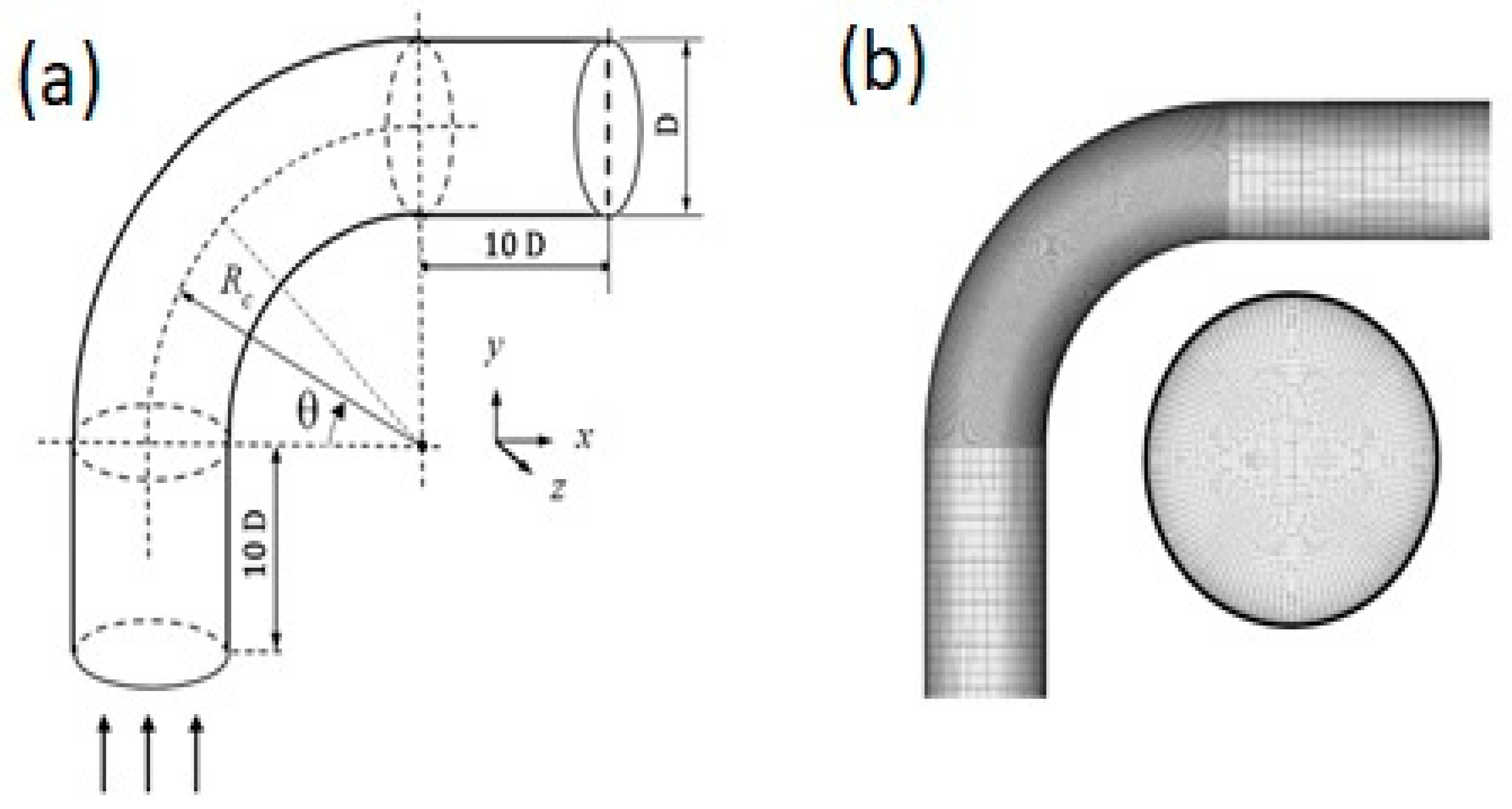
2.1. Problem Description

For three distinct Reynolds numbers {Re = (1, 5 and 10) × 10⁵}, a 90° pipe bend with a curvature ratio of (Rc/D = 2) and an inner diameter (D) is investigated in this study. The radius of the bend curvature (Rc) scaled by the bend diameter (D) is known as the curvature ratio. The Reynolds number is defined as $\mathrm{Re}=D\times u_{in}/\nu$, where u_in is the intake velocity and $\nu$ is the working fluid’s kinematic viscosity (air). For all situations in this study, a straight pipe of 10 D length is also evaluated before and after the pipe bend.

Figure 1 depicts a schematic diagram of the flow domain and the mesh configuration utilized in the current CFD investigation. The x-coordinate is defined as the axial direction downstream of the bend, the y-coordinate is defined as the direction from the inner wall to the outer wall of the bend at the bend outlet, and the z-coordinate is defined as the perpendicular direction to x and y. (u, v, w) indicate the axial, radial, and circumferential velocity components in the predefined directions (x, y, z), and different variables are non-dimensionalised utilising the bend diameter (D) and input velocity (u_in) as per the requirements, such as:

$$U=\frac{u}{u_{in}},V=\frac{v}{u_{in}},W=\frac{w}{u_{in}},V_{mag}=\frac{\sqrt{u^2+v^2+w^2}}{u_{in}},X=\frac{x}{D},Y=\frac{y}{D},Z=\frac{z}{D}$$

(1)

The velocity parameters, i.e., axial velocity, x-velocity, y-velocity and z-velocity of the fluid flow are considered as the targets in the study. The objectives of the RFR model is to accurately estimate these velocity parameters by building a function relationship with the four features, i.e., Reynolds number and the three coordinate locations of the flow.

2.2. CFD Modelling

The equations for the mass and moment balance for turbulent flows are given by Reynolds’ averaged Navier-Stokes equations for incompressible liquids, as shown in Equations (2) and (3). The standard nomenclature is used for u_i, p, ρ, μ velocity, pressure, density, and dynamic viscosity.

$$\frac{\partial u_i}{\partial x_i}=0$$

(2)

$$\rho \left(u_i\frac{\partial u_j}{\partial x_i}\right)=-\frac{\partial p}{\partial x_i}+\frac{\partial }{\partial x_i}\left[\left(\mu +{\mu }_t\right)\frac{\partial u_i}{\partial x_i}\right],j=1,2,3$$

(3)

For closure of the above equations an expression for turbulent viscosity (μ_t) is needed. In this work, k-ε model which belongs to the family of two equations RANS model is used to obtain the value of μ_t as given by

$${\mu }_t=C_{\mu }\frac{k^2}{\epsilon }$$

(4)

where c_μ is a constant that has been calculated empirically. The k-ε turbulence model is used in the current study as k-ε turbulence model has been established to give better performance for the determination of turbulent flows in pipe curvature [17,25,26,27,34]. Transport equations for k-ε model are illustrated in Equations (5) and (6), the equations also contain adjustable constants [35].

$$\frac{\partial (\rho k)}{\partial t}+\frac{\partial (\rho k{u}_i)}{\partial x_i}=\frac{\partial }{\partial x_j}\left[\left(\mu +\frac{{\mu }_t}{{\sigma }_k}\right)\frac{\partial k}{\partial x_j}\right]+P_k-\rho \epsilon$$

(5)

$$\frac{\partial (\rho \epsilon )}{\partial t}+\frac{\partial (\rho \epsilon u_i)}{\partial x_i}=\frac{\partial }{\partial x_j}\left[(\mu +\frac{{\mu }_t}{{\sigma }_{\epsilon }})\frac{\partial k}{\partial x_j}\right]+C_{1\epsilon }\frac{\epsilon }{k}{P}_k-C_{2\epsilon }\rho \frac{{\epsilon }^2}{k}$$

(6)

Here ($P_k$) signifies the production of turbulence kinetic energy and $C_{\mu }=0.09,{\sigma }_{\kappa }=1.00,{\sigma }_{\epsilon }=1.30,C_{1\epsilon }=1.44,C_{2\epsilon }=1.92$ are considered.

In the present model, at inlet of straight pipe section (upstream) the measured inlet velocity ($u=u_{in},v=0,w=0$; based on Reynolds number) is applied as the Dirichlet condition. The no-slip condition ($u=0,v=0,w=0$) was assumed at the pipe wall while the zero-stress outflow condition (i.e., with an overall mass balance correction, all flow variables have a zero-diffusion flux) was assumed at the outlet of straight pipe section in the downstream.

In present work, a three-dimensional double-precision segregated implicit solver in ANSYS Fluent 14.5, is utilised to solve the RANS equations iteratively. For momentum spatial discretization, a second-order up-wind technique is utilised. The velocities and pressures are solved using the semi-implicit pressure-linked equations (SIMPLE) technique. The solution’s convergence criteria are in the range of 10⁻⁵. Figure 1b shows a three-dimensional structured mesh with hexahedral components that is verified using a grid convergence test. Extensive attention was taken during mesh creation to ensure that the solution was correct in the area of the wall. Using the standard wall treatment function for the near wall cell employed in this work so that the value of non-dimensional distance from wall (0 < y + < 30) is tightly regulated.

2.3. RFR Modelling

Random forest regression (RFR) is a machine learning based regression method. Its foundation lies in the bagging and random subspace methods. Using bagging a number of learner trees are created which is then ensembled to obtain the overall prediction. A number of independent bootstrap samples are created from the original training data to train the learner trees. Each bootstrap sample ($D_b$) is created by drawing $n$ examples from the original training data $D$, containing $N$ examples. Replacement of examples is allowed while creating the bootstrap samples. In general, $D_b$ maybe 2/3rd of $D$ and does not contain any duplicate examples. $K$ number of independent regression trees are created for the bootstrap samples with input vector $x$. The regression trees are characterized by low bias and high variance. In regression tasks, the mean prediction of $K$ regression trees, $h_k\left(x\right)$ is calculated to obtain the random forest prediction [36].

$$\mathrm{RFR} \mathrm{prediction}=\frac{1}{K}{\displaystyle \sum }_{k=1}^K{h}_k\left(x\right)$$

(7)

Bagging is responsible for reducing the variance in the ensemble RFR model and preventing overfitting. Thus, the learner trees must not be correlated. The samples from the original training dataset which were not selected for training the $k$ th regression tree during bagging are collated to form an out-of-bag data (OOB) dataset. In general, OOB may be 1/3rd of $D$. Based on the OOB dataset the $k$ th regression tree’s performance in terms of mean squared error ($MS{E}_{OOB}$) is computed as,

$$MS{E}_{OOB}=\frac{1}{n}{\displaystyle \sum }_{i=i}^n{(y_i-{\overline{y_i}}_{OOB})}^2$$

(8)

where $y_i$ and ${\overline{y_i}}_{OOB}$ are the $i$ th prediction and the mean of $i$ th prediction from all the trees.

The coefficient of determination, i.e., $R^2{}_{OOB}$ of the OOB dataset can be computed from the $MS{E}_{OOB}$ based on the total variance, i.e., $Va{r}_y$ of the output parameter using the following relation

$$R^2{}_{OOB}=1-MS{E}_{OOB}/Va{r}_y$$

(9)

2.4. Metrics to Assess RFR Metamodel Accuracy

In this paper, a number of accuracy metrics are considered to assess the accuracy of the developed RFR metamodels. The CFD model’s output response is represented by $y_i$ and the RFR metamodel’s prediction for the corresponding output response is denoted by $\widehat{y_i}$. Thus, the residual ${\epsilon }_i$ can be computed as,

$${\epsilon }_i=y_i-\widehat{y_i}$$

(10)

Based on the mean ($\overline{y}$) of the CFD dataset the $R^2$, i.e., the coefficient of determination can be computed as,

$$R^2=1-\frac{{{\displaystyle \sum }}_{i=1}^n{\left(y_i-\widehat{y_i}\right)}^2}{{{\displaystyle \sum }}_{i=1}^n{\left(y_i-\overline{y}\right)}^2}$$

(11)

Considering the total number of the samples ($n)$, the MAE, i.e., the mean-absolute-error can be computed as,

$$\mathrm{MAE}=\frac{{{\displaystyle \sum }}_{i=1}^n\left|y_i-{\widehat{y}}_i\right|}{n}$$

(12)

Similarly, the mean-squared-error (MSE), root-mean-squared-error (RMSE), maximum error ($\mathrm{Max} \mathrm{Error}$) and median error ($\mathrm{Med} \mathrm{Error}$) are computed as,

$$\mathrm{MSE}=\frac{{{\displaystyle \sum }}_{i=1}^n{\left(y_i-{\widehat{y}}_i\right)}^2}{n}$$

(13)

$$\mathrm{RMSE}=\sqrt{\frac{{{\displaystyle \sum }}_{i=1}^n{\left(y_i-{\widehat{y}}_i\right)}^2}{n}}$$

(14)

$$\mathrm{Max} \mathrm{Error} \left(y, \widehat{y}\right)=\max . \left(\left|y_i-{\widehat{y}}_i\right|\right)$$

(15)

$$\mathrm{Med} \mathrm{Error} \left(y, \widehat{y}\right)=\mathrm{median} \left(\left|y_1-{\widehat{y}}_1\right|,\dots ,\left|y_n-{\widehat{y}}_n\right|\right)$$

(16)

3. Results and Discussion

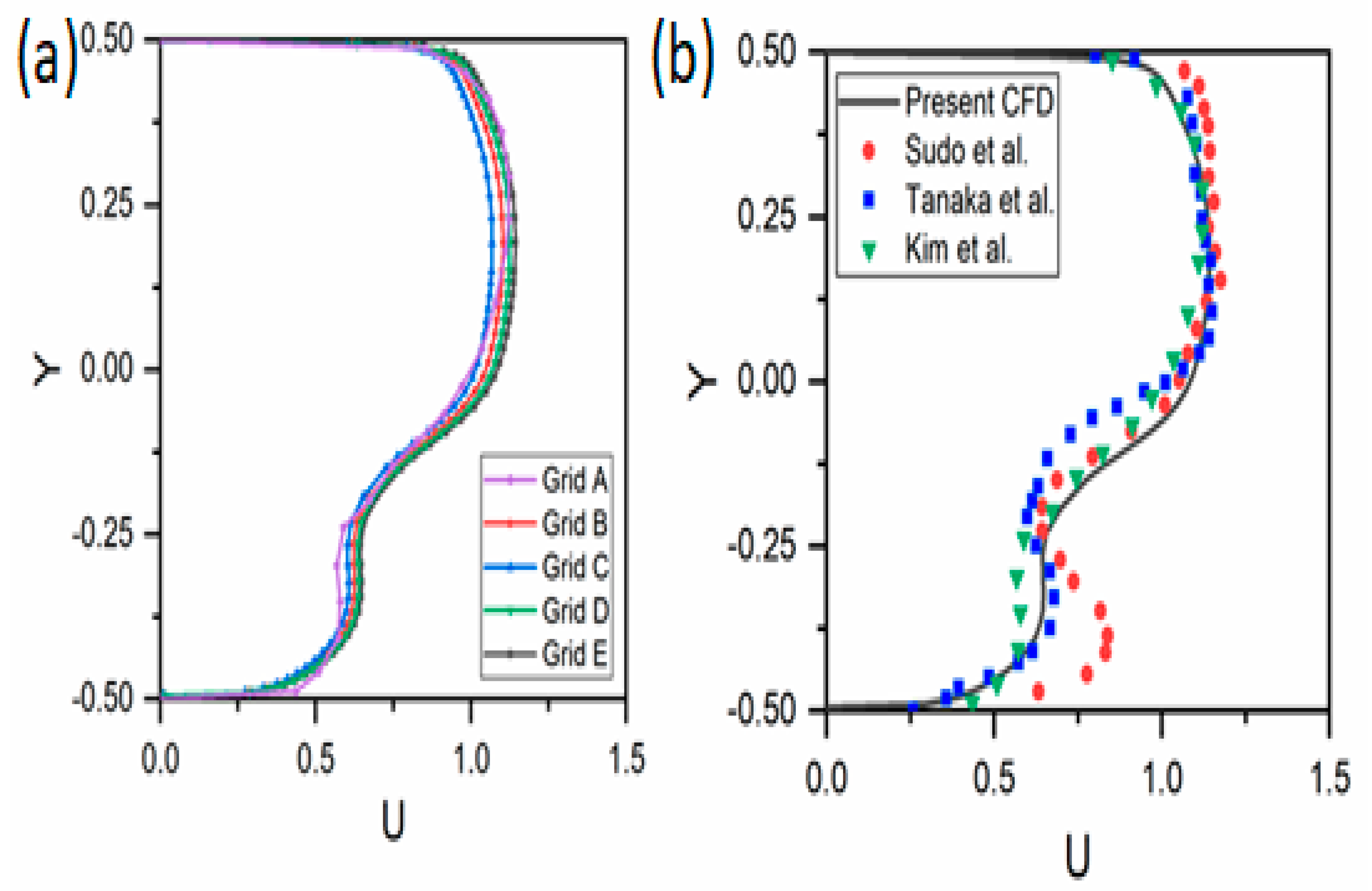
3.1. CFD Model Validation

The current CFD model and simulation setup are first confirmed against the existing experimental and numerical data in references [5,14,17] before being used to generate training and testing data using CFD models. The same geometrical arrangement and flow condition are used for that purpose. Figure 2b demonstrates that the mean axial velocity profile normalized with inlet velocity along the symmetry line at bend outlet (θ = 90°) agrees extremely well with both experimental and numerical data. There are some differences between experimental and numerical data in the bend’s inner wall area. These differences might be caused by an unfavourable pressure gradient at the bend’s inner wall. Overall, the current CFD model shows a high degree of concurrence with the existing literature results.

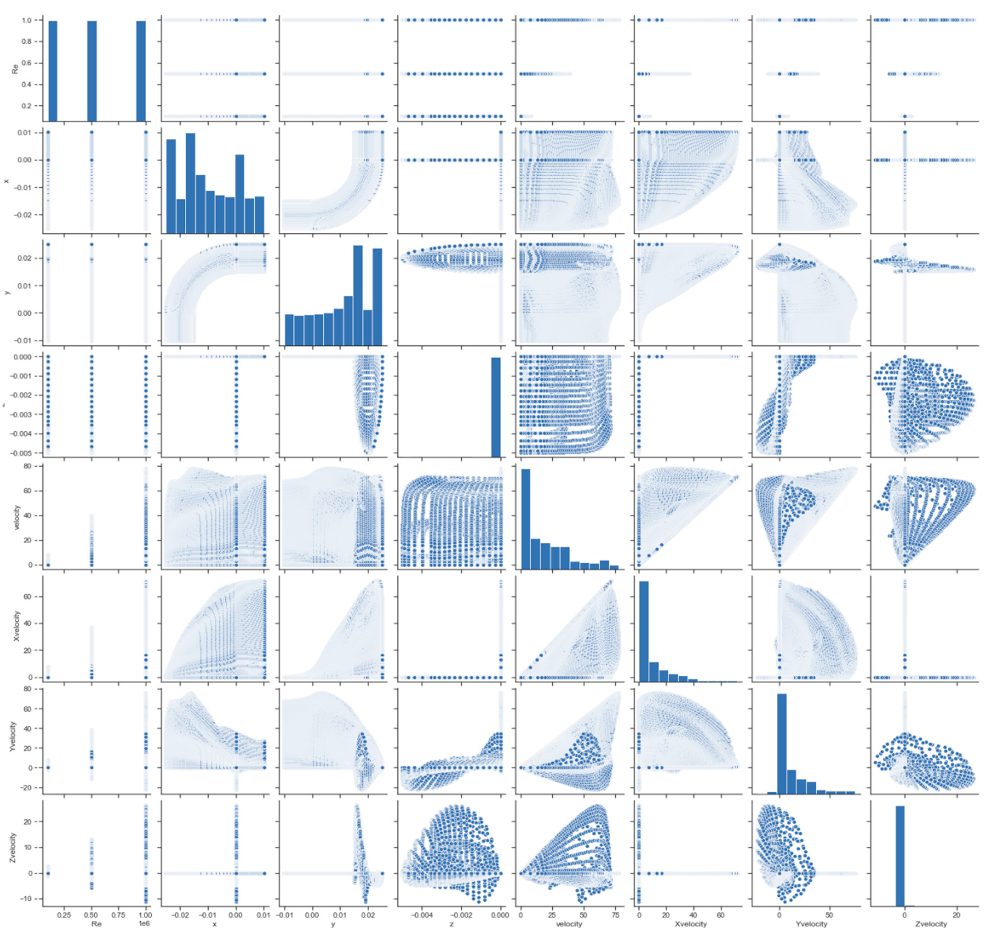
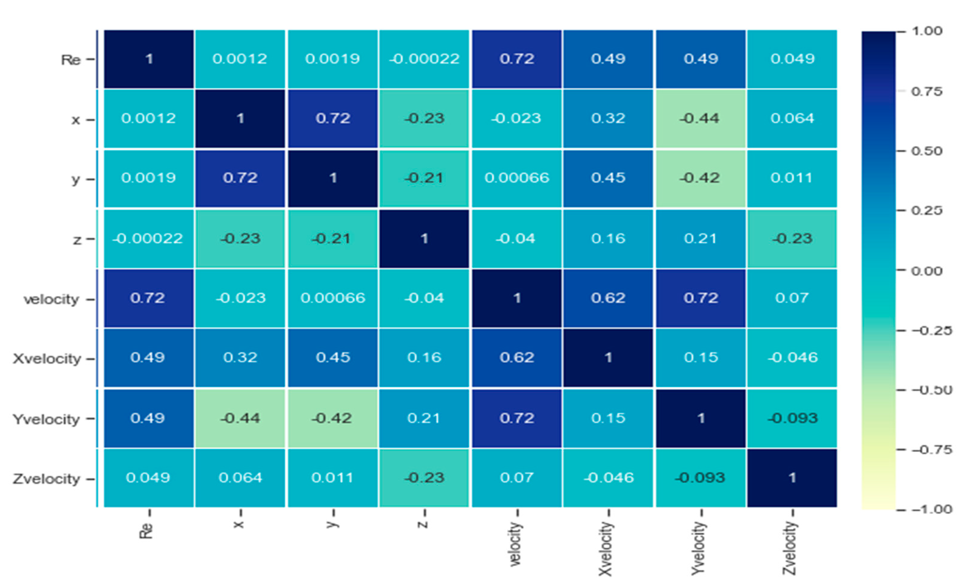
3.2. Preliminary Analysis of the Features and Targets

A large dataset of 80, 333 data points is generated by using random sampling. The data is generated using the CFD described in Section 2.2 and validated in Section 3.1. The dataset is split into 70% and 30% for training and testing, respectively. A visual assessment of the relationship between the features and the targets considered in the study is carried out by using scatter plot matrix presented in Figure 3. It is observed that there is negligible linear relationship between the features and the targets. This indicates that simple machine learning algorithms such as linear regression may be insufficient to accurately map the targets as functions of the features. Further, the Pearson’s correlation is calculated between each pair of features and targets and presented in Figure 4. Expect for a moderately high correlation (0.72) between x and y, all the other features have no correlation amongst themselves, thereby indicating the lack of any multicollinearity. Reynolds number is seen to have a moderately strong positive relationship with axial velocity and moderate positive relationship with x-velocity and y-velocity. However, Reynolds number has no correlation with z-velocity. The other features, i.e., the x, y, z coordinates have minimal correlation with the axial velocity. However, x and y coordinates share moderate relationship with x-velocity and y-velocity.

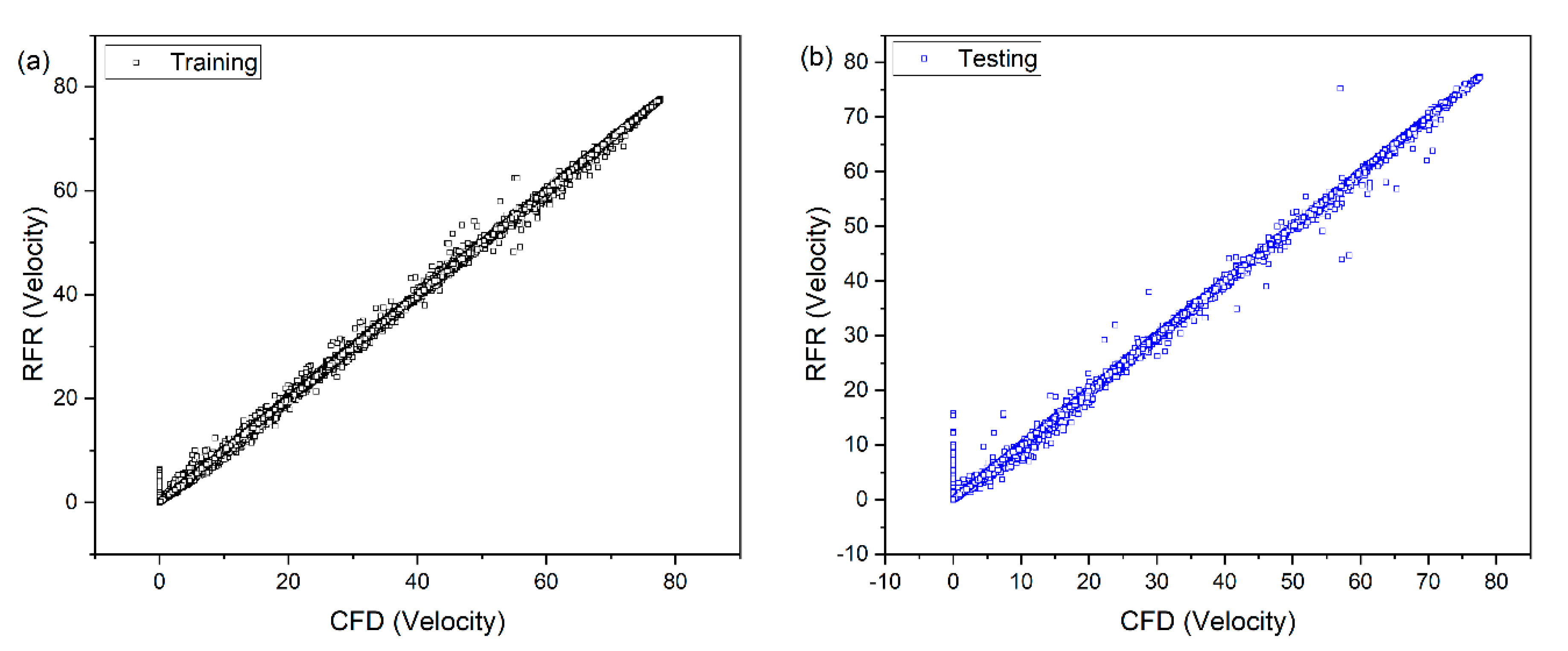
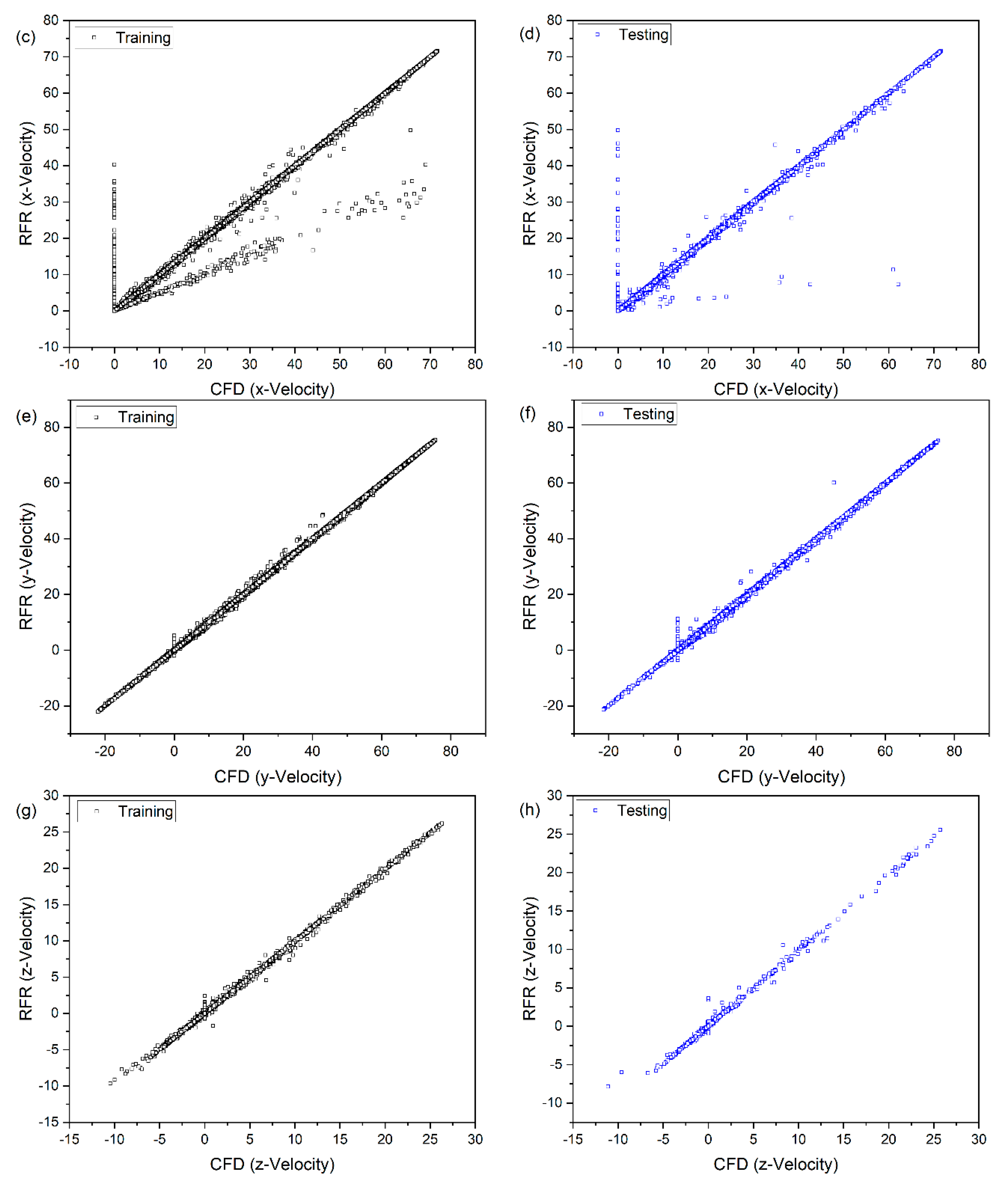
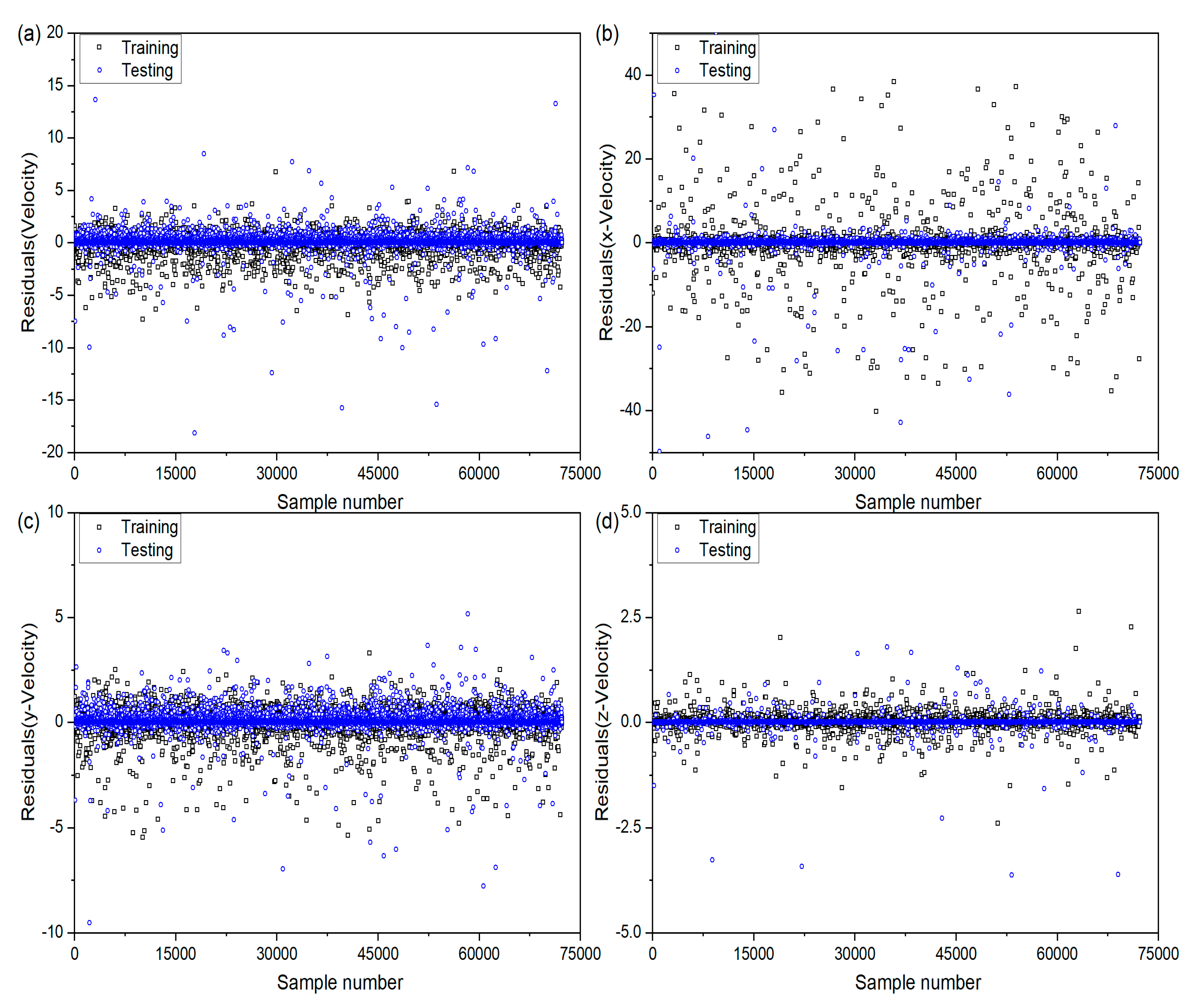
3.3. RFR Model Development and Validation

Random forest models for each target variable are developed by training on the CFD generated dataset. Since RFR models are known to be significantly influenced by the hyperparameters, a pilot study was carried out to fine tune them. Based on the hyperparameter tuning, the number of regressor is considered as 300. Figure 5 show the actual responses, i.e., the CFD values versus the RFR model predicted values of the responses. The better the prediction, closer the data point is to the diagonal line. From Figure 5, it is clear that the prediction of the axial velocity, y-velocity and z-velocity is very accurate for the training as well as testing data. A few outliers are seen in case of testing data, but the outlier deviation is not significant for axial velocity, y-velocity and z-velocity. However, x-velocity predictions show significant deviations from the true values for a number of data point. However, the performance of the x-velocity predictions is better on test data as compared to the training cases, indicating that there is no occurrence of overtraining.

To further assess the performance of the RFR models, residual analysis is carried out and presented in Figure 6. Except for the x-velocity RFR models, all other surrogate models show very small residuals. The x-velocity RFR models have relatively large residuals. However, it is encouraging to observe that in all the RFR models there is no undue cluster of residuals, indicating that there is no bias with respect to sampling order in the models. Moreover, for a very large chunk of the sample points the residual is almost zero, thereby ensuring that the models have good predictive power.

The performance of the RFR models on training and testing data is further assessed by using various metrics discussed in Section 2.3 and presented in

Table 1. Performance of the RFR models on training and testing data.

Metric	Training				Testing
	Velocity	x-Velocity	y-Velocity	z-Velocity	Velocity	x-Velocity	y-Velocity	z-Velocity
$R^2$	0.9998	0.9935	0.9999	0.9992	0.9982	0.9803	0.9991	0.9950
MSE	0.0787	1.2866	0.0389	0.0018	0.6652	3.7459	0.2572	0.0120
RMSE	0.2805	1.1343	0.1971	0.0429	0.8156	1.9354	0.5072	0.1096
MAE	0.0987	0.1250	0.0656	0.0045	0.2727	0.2646	0.1709	0.0117
Max Error	7.3217	40.3404	5.4708	2.6397	18.1603	54.7334	14.9904	3.6267
MedAE	0.0256	0.0106	0.0140	0.0000	0.0685	0.0309	0.0396	0.0000

. In all the models, there is negligible drop in the testing $R^2$ as compared to the training $R^2$, indicating absence of any over fitting while training. The performance of the RFR models on testing data in terms of other metrics such as RMSE, MAE, MedAE etc. are also encouraging.

All the CFD and RFR simulations are carried out a windows platform with Intel(R) Core(TM) i7 CPU @3.40 GHz, 16 GB RAM. The approximate computational time required for each step in the study is reported in

Table 2. Computational time requirements for CFD and RFR modelling.

Steps Involved in the Study	Computational Time (Appox., in min)
Geometry modelling	30
Meshing	15
Grid independent test	180
Validation test run	240
Present CFD and dataset generation	4800
Data cleaning and exploratory analysis	180
RFR regressor tuning study	300
RFR based modelling of all four targets	60

. It is observed that majority of the time is spend on generation of the data by the CFD models. Thus, the current approach of replacing the expensive CFD models by computationally cheaper RFR models has significant benefits. However, it should be noted that the role of CFD models cannot be completely negated, as some CFD models will be needed for generating the data needed to train the RFR models. Nevertheless, once trained on a few CFD models, the RFRs can then be used as surrogates for future CFD models to be built for similar systems, thereby leading to significant cost and effort savings.

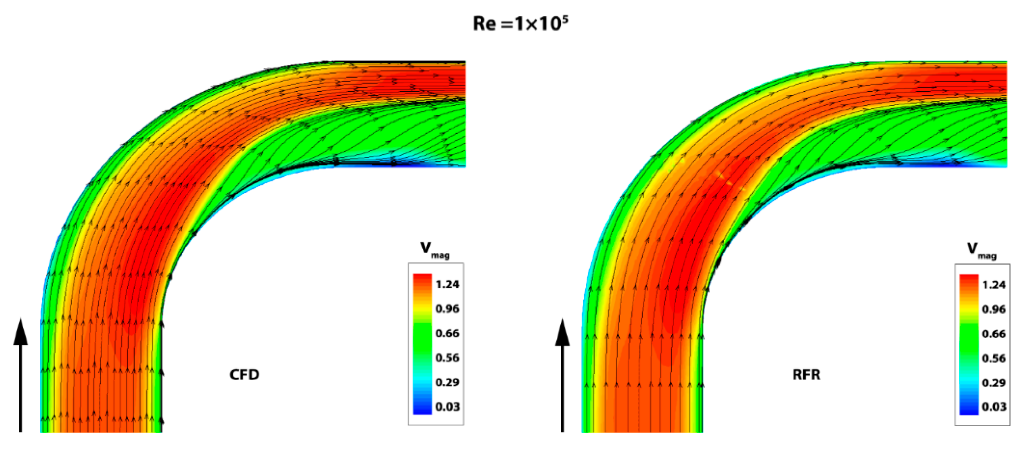
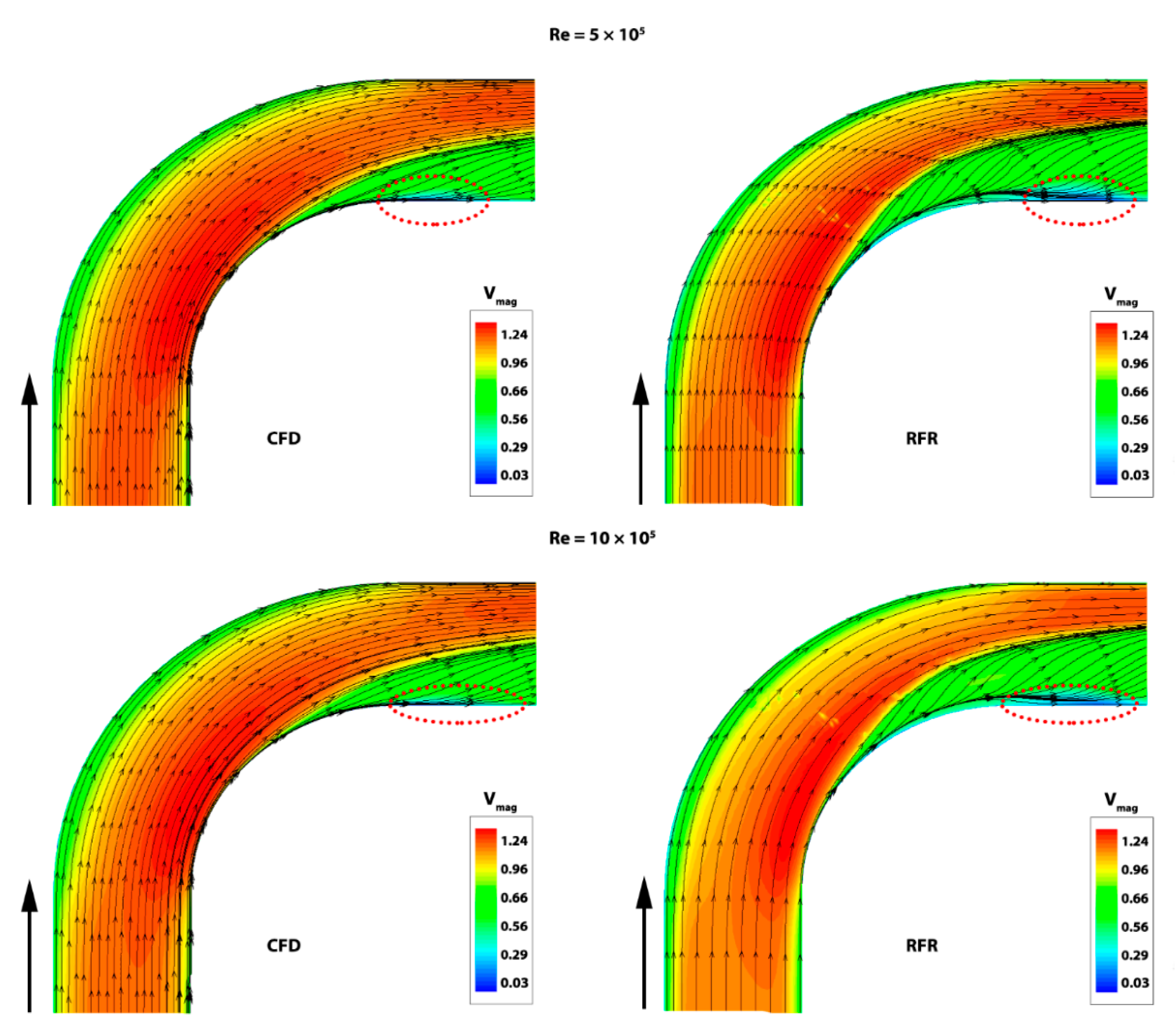
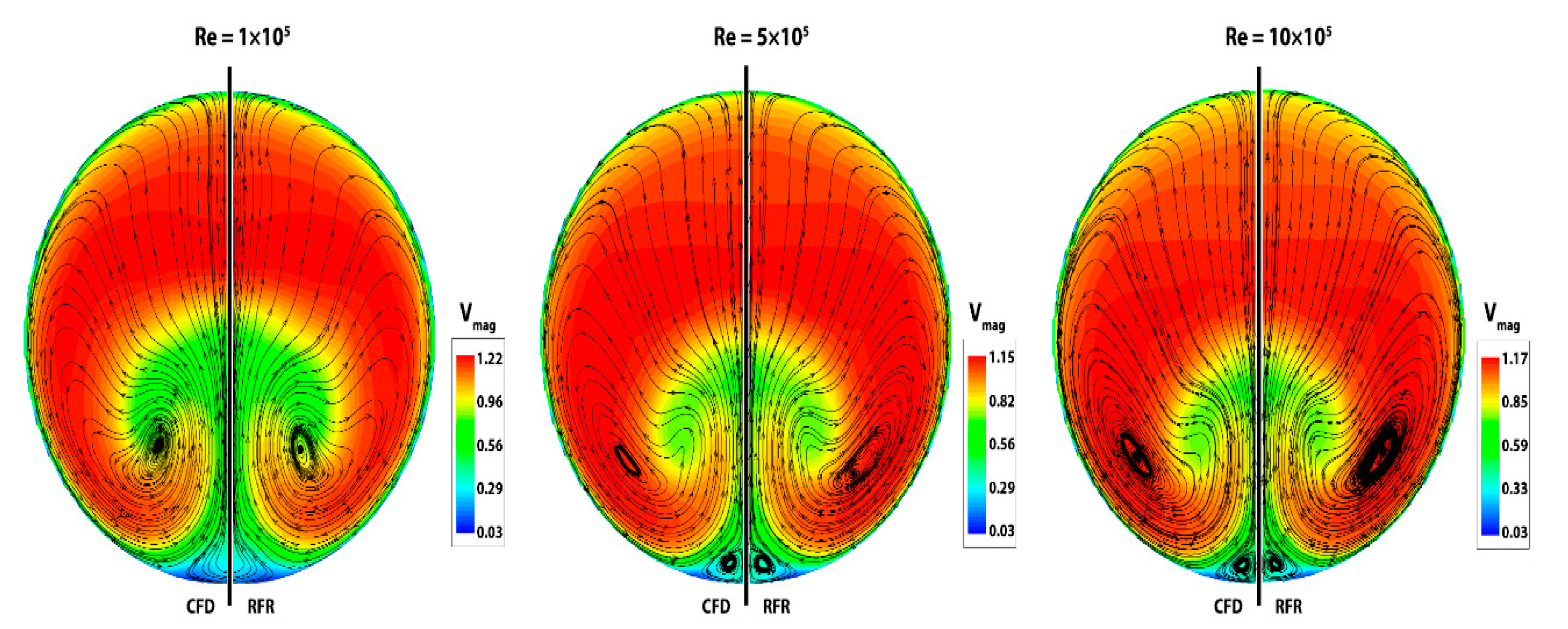
3.4. Flow Characteristics in Pipe Bends

Figure 7 and Figure 8 provide a summary of the turbulent flow inside the pipe bend at different Re which is derived from the current CFD simulations before beginning the current RFR study (left portion of each image). Figure 7 depicts streamlines in the centre flow cross-section with the time-averaged in-plane velocity magnitude normalized with the input velocity (V_mag). Flow is increased in the centre portion and flows towards the curve at the beginning of the bend (θ = 0), but the bend has no discernible impact. A flow acceleration may be noticed at the pipe’s outer wall as the flow travels ahead. Due to the formation of a high-pressure gradient between θ = 30° and 60°, this impact becomes more noticeable. The flow is moved from the centre of the pipe to the outside wall portion due to the impact of centrifugal force. Toward the wall, a time averaged flow structure with strong momentum in the centre and decreased momentum near the wall can be seen. Mean flow detaches from the inner wall area at the bend outlet (θ = 90°) and a secondary flow is visible. The existence of ‘camel back shapes’ in the profile of velocity distribution is a major feature of this flow in this area (between θ = 75° and 90°, see Figure 2). The development of secondary flow causes axial momentum loss, which results in these profiles. Turbulence along the inner wall of the bends is also considerably hindered as a result of the development of secondary flow.

Figure 8 depicts the time-averaged in-plane velocity magnitude normalised with the inlet velocity (V_mag) at the bend outlet section (θ = 90°), similar to Figure 7. The contour plot of V_mag is shown on the left side of each picture, along with the streamlines plot of mean secondary flow from the current CFD simulations. The outside wall of the bend is at the top of each image, while the inner wall is at the bottom. Supreme velocity is observed in the upper and centre regions of the bend cross section, while a low velocity area along the bend’s inner wall, as previously stated, is plainly visible. A “cross-flow boundary” occurs at the sideways wall of the bends at each Re utilised in this investigation, and the secondary flow produces a vertical velocity component that hastens the flow to the bend centre in the radial direction. For all Reynolds values, two identical counter rotating Dean vortices were discovered due to the relationship between centrifugal force with high velocity and pressure gradient on the flow. In the current study range, two distinct vortices were also seen at the inner wall portion for moderately high Re flow (for Re = 5 × 105 and 5 × 105).

Some difference between the CFD and the RFR results is observed in the prediction of low velocity region near the inner wall for high Re flow. RFR seems to be a little imprecise in this region. Moreover, minor variations in the positions of additional vortices predicted by CFD and RFR is seen. RFR does a very accurate mapping of the flow characteristics in the straight portion of the pipe but marginally underpredicts the effect of curvature at high Re flow.

4. Conclusions

This study presents an efficient machine learning based surrogate modelling approach that may be used to rapidly and accurately predict fluid flow parameters that would otherwise necessitate the use of costly CFD models. Due to its enormous practical significance and strong nonlinearity, the study of turbulent flow across pipe bends has been chosen as the topic of interest. Reynolds number and the x, y, z coordinates are chosen as the features to estimate four target variables namely axial velocity, x-velocity, y-velocity and z-velocity. The developed random forest regression machine learning model are compared with the CFD models by using various statistical metrics and graphical analysis. Overall excellent predictive ability of the RFR models is seen. However, location of certain intricate flow characteristics such as the positions of additional vortices are erroneously reported by a small margin. Nevertheless, RFR models do an excellent job in correctly mapping a complex phenomenon such as turbulent fluid flow characteristics with more than 98% accuracy. The study can be improved furthered by ascertaining the feasibility of other machine learning approaches such as Gaussian regression, XGBoost etc. Uncertainty quantification in such critical cases can be another interesting area.

References

1. Vashisth, S.; Kumar, V.; Nigam, K.D.P. A review on the potential applications of curved geometries in process industry. Ind. Eng. Chem. Res. 2008, 47, 3291–3337. [Google Scholar] [CrossRef]
2. Yamano, H.; Tanaka, M.; Murakami, T.; Iwamoto, Y.; Yuki, K.; Sago, H.; Hayakawa, S. Unsteady elbow pipe flow to develop a flow-induced vibration evaluation methodology for Japan Sodium-Cooled Fast Reactor. J. Nucl. Sci. Technol. 2011, 48, 677–687. [Google Scholar] [CrossRef]
3. Tunstall, R.; Laurence, D.; Prosser, R.; Skillen, A. Large eddy simulation of a T-Junction with upstream elbow: The role of Dean vortices in thermal fatigue. Appl. Therm. Eng. 2016, 107, 672–680. [Google Scholar] [CrossRef]
4. Kalpakli Vester, A.; Örlü, R.; Alfredsson, P.H. Turbulent flows in curved pipes: Recent advances in experiments and simulations. Appl. Mech. Rev. 2016, 68, 050802. [Google Scholar] [CrossRef]
5. Sudo, K.; Sumida, M.; Hibara, H. Experimental investigation on turbulent flow in a circular-sectioned 90-degree bend. Exp. Fluids 1998, 25, 42–49. [Google Scholar] [CrossRef]
6. Sudo, K.; Sumida, M.; Hibara, H. Experimental investigation on turbulent flow through a circular-sectioned 180 bend. Exp. Fluids 2000, 28, 51–57. [Google Scholar] [CrossRef]
7. Sudo, K.; Sumida, M.; Hibara, H. Experimental investigation on turbulent flow in a square-sectioned 90-degree bend. Exp. Fluids 2001, 30, 246–252. [Google Scholar] [CrossRef]
8. Hellström, L.H.O.; Sinha, A.; Smits, A.J. Visualizing the very-large-scale motions in turbulent pipe flow. Phys. Fluids 2011, 23, 11703. [Google Scholar] [CrossRef] [Green Version]
9. Kalpakli, A.; Örlü, R. Turbulent pipe flow downstream a 90 pipe bend with and without superimposed swirl. Int. J. Heat Fluid Flow 2013, 41, 103–111. [Google Scholar] [CrossRef]
10. De Amicis, J.; Cammi, A.; Colombo, L.P.M.; Colombo, M.; Ricotti, M.E. Experimental and numerical study of the laminar flow in helically coiled pipes. Prog. Nucl. Energy 2014, 76, 206–215. [Google Scholar] [CrossRef]
11. Mazhar, H.; Ewing, D.; Cotton, J.S.; Ching, C.Y. Measurement of the flow field characteristics in single and dual S-shape 90° bends using matched refractive index PIV. Exp. Therm. Fluid Sci. 2016, 79, 65–73. [Google Scholar] [CrossRef]
12. Cioncolini, A.; Santini, L. An experimental investigation regarding the laminar to turbulent flow transition in helically coiled pipes. Exp. Therm. Fluid Sci. 2006, 30, 367–380. [Google Scholar] [CrossRef]
13. Hayamizu, Y.; Yamamoto, K.; Yanase, S.; Hyakutake, T.; Shinohara, T.; Morita, S. Experimental study of the flow in helical circular pipes: Torsion effect on the flow velocity and turbulence. J. Therm. Sci. 2008, 17, 193–198. [Google Scholar] [CrossRef]
14. Tanaka, M.; Ohshima, H.; Monji, H. Numerical Investigation of Flow Structure in Pipe Elbow with Large Eddy Simulation Approach. In Proceedings of the ASME Pressure Vessels and Piping Conference, Prague, Czech Republic, 26–30 July 2009; pp. 449–458. [Google Scholar]
15. Hüttl, T.J.; Friedrich, R. Direct numerical simulation of turbulent flows in curved and helically coiled pipes. Comput. Fluids 2001, 30, 591–605. [Google Scholar] [CrossRef]
16. Noorani, A.; El Khoury, G.K.; Schlatter, P. Evolution of turbulence characteristics from straight to curved pipes. Int. J. Heat Fluid Flow 2013, 41, 16–26. [Google Scholar] [CrossRef]
17. Kim, J.; Yadav, M.; Kim, S. Characteristics of secondary flow induced by 90-degree elbow in turbulent pipe flow. Eng. Appl. Comput. Fluid Mech. 2014, 8, 229–239. [Google Scholar] [CrossRef]
18. Röhrig, R.; Jakirlić, S.; Tropea, C. Comparative computational study of turbulent flow in a 90 pipe elbow. Int. J. Heat Fluid Flow 2015, 55, 120–131. [Google Scholar] [CrossRef]
19. Takamura, H.; Ebara, S.; Hashizume, H.; Aizawa, K.; Yamano, H. Flow visualization and frequency characteristics of velocity fluctuations of complex turbulent flow in a short elbow piping under high Reynolds number condition. J. Fluids Eng. 2012, 134, 101201. [Google Scholar] [CrossRef]
20. Dutta, P.; Saha, S.K.; Nandi, N. Numerical study of curvature effect on turbulent flow in 90 pipe bend. In Proceedings of the International Conference on Theoretical, Applied, Computational and Experimental Mechanics ICTACEM-2014/028, Kharagpur, India, 29–31 December 2014. [Google Scholar]
21. Dutta, P.; Saha, S.K.; Nandi, N. Computational study of turbulent flow in pipe bends. Int. J. Appl. Eng. Res. 2015, 19, 5–16. [Google Scholar]
22. Dutta, P.; Nandi, N. Study on pressure drop characteristics of single phase turbulent flow in pipe bend for high reynolds number. ARPN J. Eng. Appl. Sci. 2015, 10, 11. [Google Scholar]
23. Dutta, P.; Nandi, N. Effect of Reynolds number and curvature ratio on single phase turbulent flow in pipe bends. Mech. Mech. Eng. 2015, 19, 5–16. [Google Scholar]
24. Dutta, P.; Nandi, N. Effect of bend curvature on velocity & pressure distribution from straight to a 90 pipe bend-A Numerical Study. REST J. Emerg. Trends Model. Manuf. 2016, 2, 103–108. [Google Scholar]
25. Dutta, P.; Saha, S.K.; Nandi, N.; Pal, N. Numerical study on flow separation in 90° pipe bend under high Reynolds number by k-ε modelling. Eng. Sci. Technol. Int. J. 2016, 19, 904–910. [Google Scholar] [CrossRef] [Green Version]
26. Dutta, P.; Nandi, N. Numerical study on turbulent separation reattachment flow in pipe bends with different small curvature ratio. J. Inst. Eng. Ser. C 2019, 100, 995–1004. [Google Scholar] [CrossRef]
27. Dutta, P.; Nandi, N. Numerical analysis on the development of vortex structure in 90° pipe bend. Prog. Comput. Fluid Dyn. Int. J. 2021, 21, 261. [Google Scholar] [CrossRef]
28. Gamahara, M.; Hattori, Y. Searching for turbulence models by artificial neural network. Phys. Rev. Fluids 2017, 2, 54604. [Google Scholar] [CrossRef]
29. Gholami, A.; Bonakdari, H.; Zaji, A.H.; Michelson, D.G.; Akhtari, A.A. Improving the performance of multi-layer perceptron and radial basis function models with a decision tree model to predict flow variables in a sharp 90 bend. Appl. Soft Comput. 2016, 48, 563–583. [Google Scholar] [CrossRef]
30. Rahimi, M.; Hajialyani, M.; Beigzadeh, R.; Alsairafi, A.A. Application of artificial neural network and genetic algorithm approaches for prediction of flow characteristic in serpentine microchannels. Chem. Eng. Res. Des. 2015, 98, 147–156. [Google Scholar] [CrossRef]
31. Srinivasan, P.A.; Guastoni, L.; Azizpour, H.; Schlatter, P.; Vinuesa, R. Predictions of turbulent shear flows using deep neural networks. Phys. Rev. Fluids 2019, 4, 54603. [Google Scholar] [CrossRef] [Green Version]
32. Ganesh, N.; Dutta, P.; Ramachandran, M.; Bhoi, A.K.; Kalita, K. Robust metamodels for accurate quantitative estimation of turbulent flow in pipe bends. Eng. Comput. 2019, 36, 1041–1058. [Google Scholar] [CrossRef]
33. Narayanan, G.; Joshi, M.; Dutta, P.; Kalita, K. PSO-tuned support vector machine metamodels for assessment of turbulent flows in pipe bends. Eng. Comput. 2019, 37, 981–1001. [Google Scholar] [CrossRef]
34. Homicz, G.F. Computational Fluid Dynamic Simulations of Pipe Elbow Flow; Sandia National Laboratories: Los Angeles, CA, USA, 2004. [Google Scholar]
35. Tu, J.; Yeoh, G.H.; Liu, C. Computational Fluid Dynamics: A Practical Approach; Butterworth-Heinemann: Oxford, UK, 2018; ISBN 0081012446. [Google Scholar]
36. Seo, D.K.; Kim, Y.H.; Eo, Y.D.; Park, W.Y.; Park, H.C. Generation of radiometric, phenological normalized image based on random forest regression for change detection. Remote Sens. 2017, 9, 1163. [Google Scholar] [CrossRef] [Green Version]
Figure 1. (a) Schematic diagram of the flow domain and (b) present CFD model with computational grid.
Processes 09 02095 g001
Figure 2. Assessment of normalized axial velocity profile at bend outlet (a) grid convergence test (b) validation of the present CFD model.
Processes 09 02095 g002
Figure 3. Scatter plot matrix of the feature and the targets.
Processes 09 02095 g003
Figure 4. Correlation heat map between features and targets.
Processes 09 02095 g004
Figure 5. CFD versus RFR predicted velocity parameters for training (subfigure (a,c,e,g)) and testing (subfigure (b,d,f,h)) data. (a,b) axial velocity (c,d) x-velocity (e,f) y-velocity (g,h) z-velocity.
Processes 09 02095 g005aProcesses 09 02095 g005b
Figure 6. Prediction residuals while training and testing the RFR models for different target variables (a) velocity (b) x-velocity (c) y-velocity (d) z-velocity.
Processes 09 02095 g006
Figure 7. Flow structure at central cross-section of the bend for different Re. (left section: CFD result; right section: RFR result). The oval shaped red dotted lines indicate the region in which maximum discrepancy in CFD and RFR results is observed.
Processes 09 02095 g007aProcesses 09 02095 g007b
Figure 8. Flow structure at bend outlet (θ = 90°) of the bend for different Re. (left section: CFD result; right section: RFR result).
Processes 09 02095 g008