
Applicability of Constitutive Models to Describing the Compressibility of Mining Backfill: A Comparative Study


Research Institute on Mines and Environment (RIME UQAT-Polytechnique), Department of Civil, Geological and Mining Engineering, École Polytechnique de Montréal, C.P. 6079 Succursale Centre-Ville, Montréal, QC H3C 3A7, Canada
*
Author to whom correspondence should be addressed.
Processes 2021, 9(12), 2139; https://0-doi-org.brum.beds.ac.uk/10.3390/pr9122139
Submission received: 25 October 2021
/
Revised: 12 November 2021
/
Accepted: 22 November 2021
/
Published: 26 November 2021
(This article belongs to the Special Issue Numerical Modeling in Civil and Mining Geotechnical Engineering)
Abstract
:The compressibility of mining backfill governs its resistance to the closure of surrounding rock mass, which should be well reflected in numerical modeling. In most numerical simulations of backfill, the Mohr–Coulomb elasto-plastic model is used, but is constantly criticized for its poor representativeness to the mechanical response of geomaterials. Finding an appropriate constitutive model to better represent the compressibility of mining backfill is critical and necessary. In this paper, Mohr–Coulomb elasto-plastic model, double-yield model, and Soft Soil model are briefly recalled. Their applicability to describing the backfill compressibility is then assessed by comparing numerical and experimental results of one-dimensional consolidation and consolidated drained triaxial compression tests made on lowly cemented backfills available in the literature. The comparisons show that the Soft Soil model can be used to properly describe the experimental results while the application of the Mohr–Coulomb model and double-yield model shows poor description on the compressibility of the backfill submitted to large and cycle loading. A further application of the Soft Soil model to the case of a backfilled stope overlying a sill mat shows stress distributions close to those obtained by applying the Mohr–Coulomb model when rock wall closure is absent. After excavating the underlying stope, rock wall closure is generated and exercises compression on the overlying backfill. Compared to the results obtained by applying the Soft Soil model, an application of the Mohr–Coulomb model tends to overestimate the stresses in the backfill when the mine depth is small and underestimate the stresses when the mine depth is large due to the poor description of fill compressibility. The Soft Soil model is recommended to describe the compressibility of uncemented or lightly cemented backfill with small cohesions under external compressions associated with rock wall closure.
1. Introduction
Backfill is being considered as an integral part of several underground mining methods. It is used as working platform in overhand cut-and-fill mining method or for creating safer working space in underhand cut-and-fill mining method. Using mine waste as underground mining backfill helps to minimize the surface disposal of mine waste [1,2,3,4]. However, the main objective of backfilling the mined-out spaces is to effectively control the rock wall closure and maintain the regional ground stability [5,6,7,8,9]. The compressibility of backfill plays an important role in resisting the closure of surrounding rock walls associated with adjacent extraction or/and creep behavior. Previous studies showed that a backfill of low compressibility can carry significant stresses generated by walls convergence and provide considerable support to surrounding rocks [6,10,11,12,13]. In underground mines, especially with overhand cut-and-fill or open stoping methods, however, the commonly used backfill is uncemented or has a low-cement content. The compressibility is large under low compression state and decreases as the compression increases. Understanding and properly describing the compressibility of mining backfill is thus of specific interest for mining industry to evaluate fill performance and stability of underground structures.
Numerical modeling provides an efficient and cost-effective method to study the complex mechanical behavior of backfill. Nonetheless, the reliability and applicability of a numerical model largely depends on the capability of applied constitutive model. There are many constitutive models of geomaterial proposed in literatures with various levels of complexity [14,15,16,17]. Until now, the Mohr–Coulomb elasto-plastic model is the most used one to simulate the mining backfill due to the simplicity and clear physical meaning of model parameters [18,19,20,21,22,23,24,25]. The justification of the Mohr–Coulomb model is usually attributed to the good fit with the shear strength of backfill [26,27,28,29,30]. However, it is well-known that the Mohr–Coulomb elasto-plastic model suffers from its linearly elasticity and the neglect of volumetric yielding. In reality, geomaterial can have a nonlinear behavior before yielding while a mining backfill can become denser upon a large compression generated by wall closure. Given the restrictions of the Mohr–Coulomb elasto-plastic model, it remains unknown which constitutive model should be applied to better represent the compressibility of mining backfill.
There are few research studies devoted toward identifying a constitutive model applicable to describing the compressibility of mining backfill. Among these studies, Oliver and Landriault [31] investigated the convergence resistance of backfill by simulating an oedometer test of dense sand with the Mohr–Coulomb model and the strain-softening model. Different values of Young’s modulus and Poisson’s ratio were applied. Results show that numerical model remains elastic over the full strain range except when a very small Poisson’s ratio is applied. The predicted compressive stresses obtained with the two constitutive models are almost identical and significantly smaller than the experimental results. Clark [32] reproduced the non-linear stress–strain response of the dewatered tailings backfill in uniaxial compression tests with a cap model in FLAC. The input parameters for the cap model were obtained by applying the curve fitting on all the experimental results. The good agreements between the numerical model and experimental results do not mean that the calibrated numerical model can be used to correctly predict the mechanical behavior of the backfill under an untested stress condition. Fourie et al. [33] performed a finite element analysis by making use of the linearly elastic, Mohr–Coulomb, Drucker-Prager, and modified Cam-Clay models to simulate a backfilled stope at depth of 2000 m below the ground surface. The hanging wall convergence for the modified Cam-Clay model was found to be 11% larger than the results obtained with the other three models due to the plastic volumetric strain of backfill. The numerical results were not further compared with physical test data. Lagger et al. [34] used the double-yield model in FLAC3D to simulate the oedometer test of pea gravel as a filling material. The cap pressure of the double-yield model was calibrated based on the experimental results in a stress range of 0 to 6 MPa. Within this range, numerical results reasonably correlate with the test data, but the comparisons for the higher load stage was not shown. Therefore, more works are necessary to identify a suitable constitutive model to describe the compressibility of mining backfill, particularly by analyzing its predictive capability and comparing with physical results.
In this study, the Mohr–Coulomb elasto-plastic, double-yield, and Soft Soil models were recalled. Their abilities to describe the compressibility of backfill were assessed by comparing the numerical results obtained using FLAC3D with the experimental results of one-dimensional consolidation and consolidated drained triaxial compression tests of lowly cemented backfill available in the literature. Some unknown model parameters were calibrated based on part of the experimental results, and the calibrated models were applied to predict the other part of the experimental results. The identified model was then benchmarked with the Mohr–Coulomb model in simulating a backfilled stope, overlying a sill mat at different mine depths. The applicability of the identified model and the significance of modeling fill compressibility will be shown and discussed. In addition, validations of FLAC3D against analytical solutions of a cylinder hole in the linearly elastic and Mohr–Coulomb material and the sensitivity analyses of the numerical models are provided in the Appendix A, Appendix B and Appendix C.
2. Commonly Used Constitutive Models in Geotechnical Engineering
For the sake of completeness, a few constitutive models commonly used in geotechnical engineering, including the Mohr–Coulomb elasto-plastic, double-yield, and Soft Soil models, are briefly recalled. Compression stresses are positive and tension is negative. All strength parameters are in terms of effective stresses.
2.1. Mohr–Coulomb Elasto-Plastic Model
The Mohr–Coulomb elasto-plastic model considers a material as linearly elastic and perfectly plastic once the stress state reaches a state of yield [35]. It is the most commonly used constitutive model in modeling the mechanical behavior of mining backfill.
Figure 1 shows the envelope of the Mohr–Coulomb model in p–q space (Figure 1a) and the typical stress–strain relation (Figure 1b). In the figure, ϕ and c are the friction angle and cohesion, respectively; εq is the deviatoric strain; p and q are the mean and deviatoric stresses, respectively, expressed as:
where σ1, σ2, and σ3 are the major, intermediate and minor principal stresses, respectively.
The linear stress–strain relation in the elastic regime (below the envelope) is described using a constant Young’s modulus E and Poisson’s ratio ν and assumed to follow Hooke’s law. Once the stress state reaches the yield envelop defined by the Mohr–Coulomb criterion, infinite plastic shear strain occurs under a constant load.
The stress–strain relation in the elastic regime is expressed as:
where σx, σy, σz, τxy, τyz, τxz are the components of stress tensor; εx, εy, εz, γxy, γyz, γxz are the components of the strain tensor.
The well-known Mohr–Coulomb criterion is expressed as follows, to relate shear strength τ and the corresponding normal stress σ [36,37]:
or as follows, in terms of principal stresses:
A 3D generalization of Equation (8) in terms of stress invariants is given as [38]:
where θl is the Lode angle.
The Mohr–Coulomb criterion correlates well with the shear strength of backfill, but tends to overestimate the tensile strength [39]. A tensile strength T smaller than that calculated by applying the equation of Mohr–Coulomb, called tension cut-off and, thus, usually applies for mining backfill. An associated or non-associated flow rule can be applied by varying the value of dilation angle ψ to model the plastic volume change due to shearing. The Mohr–Coulomb model does not capture the plastic volumetric strain under isotropic compression.
2.2. Double-Yield Model
The double-yield model was built in FLAC [40], which involves shear and tensile yield criteria of the Mohr–Coulomb model, and a volumetric yield surface. Its stress–strain relation in the elastic region is described by Hooke’s law. Figure 2 illustrates the schematic yield surface and stress–strain behavior of the double-yield model.
The volumetric yield surface (or cap) of the double-yield model shown in Figure 2a is independent on the deviatoric stress, and is defined as:
where pc is the current cap pressure (or preconsolidation pressure).
The double-yield model has an associated volumetric flow rule and its hardening rule relates to the plastic volumetric strain through a defined piecewise-linear function. The prescribed piecewise-linear function is flexible, but needs to be calibrated based on the results of physical tests. The bulk modulus K in the double-yield model is proportional to the derivative of cap hardening function as:
where R is a constant.
Equation (11) indicates that the elastic modulus of the double-yield model is dependent on a piecewise-linear function of the cap pressure, which explains the varied slope of the stress–strain curve in the elastic region, as shown in Figure 2b. Compared with the Mohr–Coulomb model, the double-yield model involves a volumetric yield surface, which enables accounting the plastic volumetric strain due to the mean stress. The double-yield model has been adopted in some studies to simulate the mechanical performance of considerably compressible backfill material [34,41].
2.3. Soft Soil Model
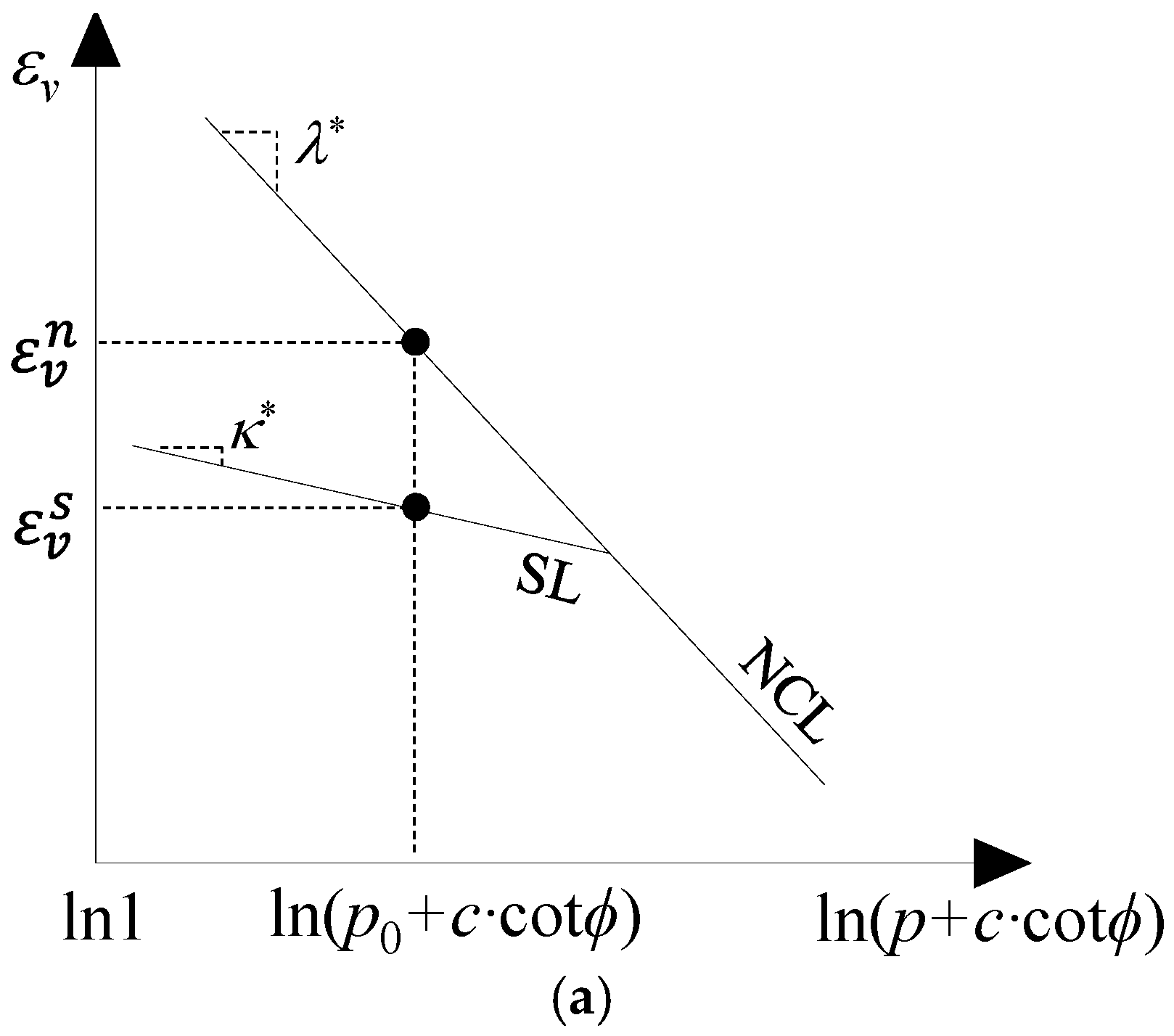
The Soft Soil model is an advanced Cam-Clay type model [14,42] based on the critical state concept [43] and captures the irreversible void change accompanying the soil deformation. Figure 3a shows the relation between the volumetric strain εv and mean stress p in the Soft Soil model. It is postulated that εv linearly reduces with the increase of p along a normal consolidation line (NCL) in the semi-logarithmic space. The NCL has a slope of λ*. For unloading and reloading, εv varies following an elastic swelling line (SL) with a slope of κ*. In the figure, p0 is a reference value of mean stress. is the reference volumetric strain corresponding to (p0 + c∙cotϕ) on the NCL and is the reference volumetric strain corresponding to (p0 + c∙cotϕ) on the SL. The equations for NCL and SL in the Soft Soil model are given as:
Figure 3b,c show the yield surface and stress–strain relation of the Soft Soil model. The yield surface consists of the envelope of the Mohr–Coulomb model and an elliptical cap. The elliptical cap has an apex on a critical state line as shown in Figure 3b and its formulation is expressed as:
where Ms is the slope of the critical state line in p–q space, which can be calculated based on the flow rule of the modified Cam-Clay model [42,44] as:
where K0 is the coefficient of earth pressure at-rest in normally consolidated condition.
The Soft Soil model employs an associated flow rule for the volumetric yield surface. The hardening of the volumetric yield surface is attributed to the plastic volumetric strain and is defined as:
The elastic modulus in the Soft Soil model is mean stress-dependent expressed as:
The Soft Soil model can be considered as a combination of the Mohr–Coulomb criterion and the modified Cam-Clay model. The critical state line in the Soft Soil model controls the shape of yield surface while the shear strength is defined by the Mohr–Coulomb envelope. The Soft Soil model has been used in a few studies to analyze the compressibility of soft clay [45,46], but has rarely been applied for mining backfill.
3. Comparisons between Numerical Models and Laboratory Tests
The applicability of constitutive models presented above to describing the compressibility of mining backfill, is identified by modeling one-dimensional consolidation and consolidated drained triaxial compression tests made on lowly cemented backfill available in the literature using FLAC3D [40].
3.1. Comparison with One-Dimensional Consolidation Tests
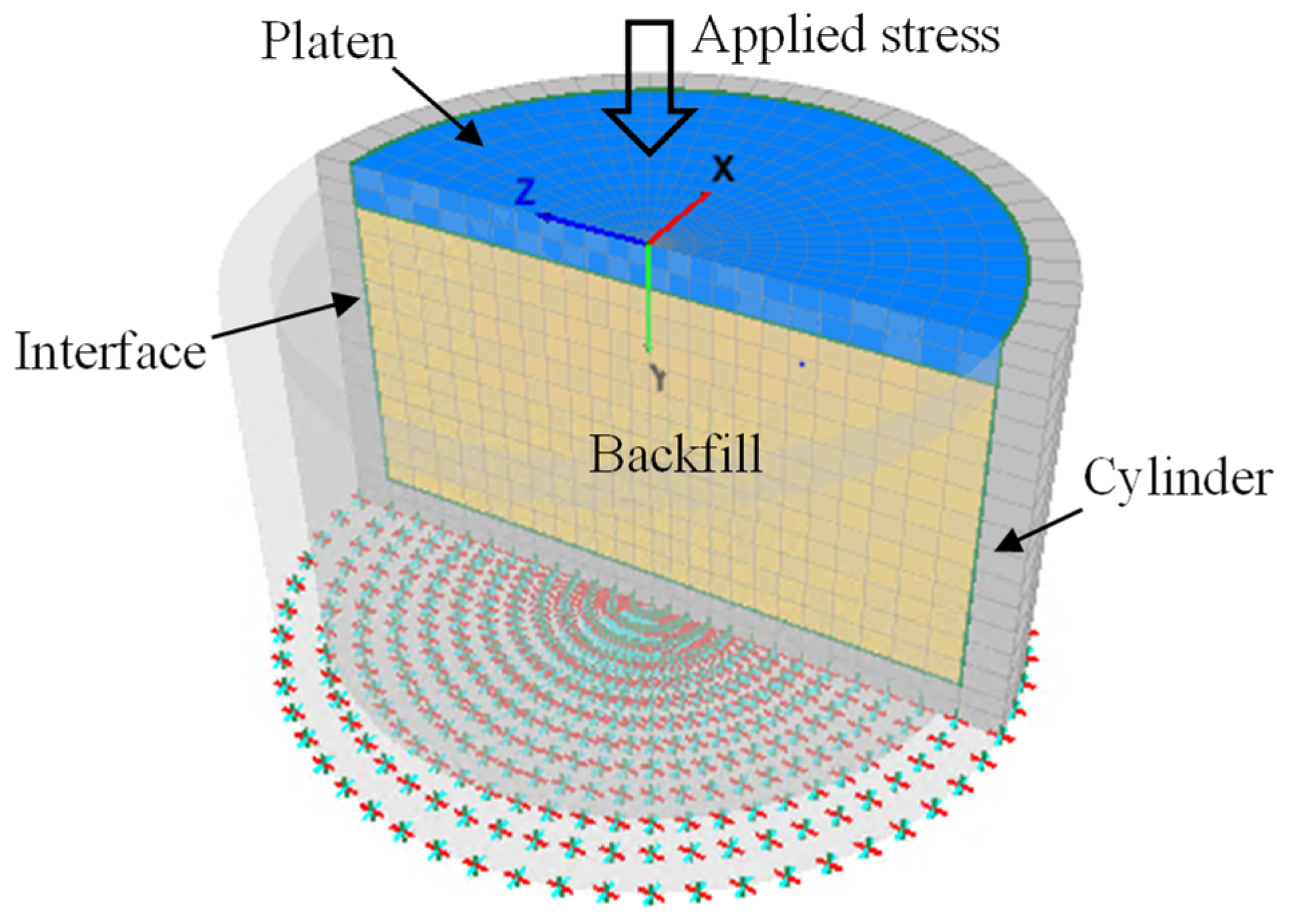
Pierce [26] conducted one-dimensional consolidation tests on Golden Giant paste backfill. The backfill samples were made by mixing the tailings with 3% binder by weight and cured for 28 days. Samples were casted in a rigid metal cylinder, which also acted as a confining ring in the consolidation tests. The backfill samples have a diameter of 75 mm and a height of around 37.5 mm. The measured properties include a density ρ of 2013 kg/m3, a porosity n of 49%, a cohesion c of 40 kPa and a friction angle ϕ of 41°. During the consolidation tests of Pierce [26], a porous stone was put under the cylinder to allow drainage and a platen was placed on the top of the cylinder for the incremental load. Figure 4 shows the physical model and the laboratory results of the applied stress–compressive strain curve of one-dimensional consolidation tests conducted by Pierce [26]. The loading path has four stages, involving an increase from 0 to 4 kN in an increment of 0.5 kN, a decrease from 4 to 1 kN in an increment of 1 kN, an increase from 1 to 6 kN in an increment of 1 kN, and an increase from 6 to 12 kN in an increment of 2 kN.
Figure 5 shows a numerical model of a one-dimensional consolidation test constructed with FLAC3D, which involves a backfill sample, a cylinder (cell) and a loading platen. The platen is built to allow loading on a displacement boundary of the top surface. The numerical model shown in Figure 5 has the identical dimensions as the physical model of Pierce [26]. The mesh size of the numerical model is 3 mm based on the sensitivity analyses. Both the cylinder and platen are modeled as linear elastic material with a Young’s modulus of 200 GPa and a Poisson’s ratio of 0.3. The Mohr–Coulomb, double-yield, and Soft Soil models are applied for the backfill sample to make comparisons. Interface elements are applied between the cylinder and backfill. The normal and shear stiffness of the interface are determined based on an equation recommended in the FLAC3D manual [40]. The interface friction angle ϕi is taken as 2/3 of ϕ, while its cohesion ci is assumed equal to c of backfill [47,48]. The displacements on the bottom of the model are restricted and other boundaries are set free. The same loading path in Pierce [26] tests is applied in the numerical simulations while the average normal displacement on the top of platen is recorded to calculate the compressive strain for different applied stresses.
In the numerical simulations, the Poisson’s ratio of backfill is related to its friction angle through ν = (1 − sinϕ)/(2 − sinϕ) by considering a unique value of at-rest earth pressure coefficient K0 [49,50].The tensile strength T of backfill is taken as 1/10 of its uniaxial compressive strength (UCS) [39]. The initial value of void ratio eini is calculated based on the measured porosity. However, some parameters remain unknown including K and shear modulus G for the Mohr–Coulomb model, R and the piecewise-linear function of pc for the double-yield model, λ*, κ*, and pc for the Soft Soil model. These parameters are determined by calibrating the numerical results based on part of laboratory results of Pierce [26] associated with the loading paths 1 and 2 as shown in Figure 4. Table 1 summarizes all parameters applied for different constitutive models. Numerical models with the calibrated parameters are then called the calibrated models, which are further applied to predict the other part of laboratory results associated with loading paths 3 and 4.
Figure 6 shows the comparisons between the laboratory results of one-dimensional consolidation tests reported by Pierce [26] and the numerical results by applying the Mohr–Coulomb (Figure 6a), double-yield (Figure 6b), and Soft Soil (Figure 6c) models for backfill. In Figure 6a, one sees the compressive strain of the Mohr–Coulomb model linearly increases as the applied stress increases. For the unloading stage, the stress–strain curve of the Mohr–Coulomb model is almost parallel to that in the loading stage. The minor scatter between the curves of loading and unloading is attributed to the yield of fill-wall interface. However, the experimental strain shows nonlinear relation with the applied stress in the test while only a small component of compressive strain is reversible at the unloading stage. The poor agreement between numerical and laboratory results is explained as that the Mohr–Coulomb model simulates a constant elastic modulus and does not capture the volumetric yield of backfill.
Figure 6b shows that the calibrated results of the double-yield model correlate well with the laboratory results, but the predicted compressive strain steeply increases as the applied stress further increases. It is because that the prescribed piecewise-linear function of the cap pressure in the double-yield mode is calibrated, based on part of the laboratory results. The prescribed function is flexible and can result in a good fit between the numerical and test results. However, when the applied stress exceeds the range of prescribed function, the double-yield model demonstrates infinite plastic volumetric strain as shown in Figure 6b. The predictive capability of the double-yield model is thus limited when the test data for calibration are insufficient. For the Soft Soil model, Figure 6c illustrates that both the described and predicted numerical results agree well with the laboratory results. Minor difference between the described results of the Soft Soil model and test results is seen when the applied stress is smaller than 230 kPa. This is because that the cementation in the backfill increases its primary stiffness at a small stress level. As the applied stress increases, the cement bond yields as shown by a drop of fill stiffness in Figure 6c. The mechanical behavior of cemented backfill then approaches an uncemented condition. In the Soft Soil models, the large primary stiffness caused by the cement bond at the small stress level can be pseudo-simulated by using an overconsolidation state, though their mechanisms are different. The Soft Soil model is thus deemed capable of describing the compressibility of lightly cemented or uncemented backfill in a confined compression condition.
3.2. Comparison with Consolidated Drained Triaxial Compression Tests
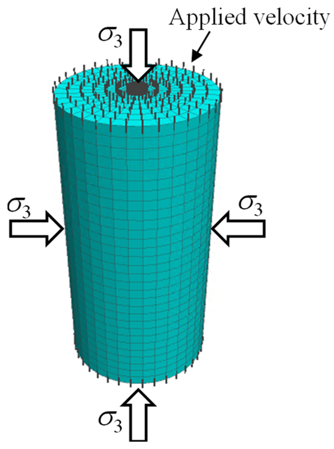
Rankine [28] conducted consolidated drained triaxial compression tests on Cannington paste backfill. The backfill samples have a diameter of 38 mm, a height of 76 mm, a cement content of 2%, a solid content of 74% by weight, and were cured for 28 days. The density of backfill is 2091 kg/m3 and the porosity is 51.2%. Figure 7 shows the physical model and deviatoric stress–strain curve of consolidated drained triaxial compression tests under confining pressures of 100, 200, 500 kPa performed by Rankine [28].
Figure 8 illustrates a numerical model of backfill sample built with FLAC3D in simulations of consolidated drained triaxial compression tests. The numerical model has same sizes as the samples of Rankine [28], while the mesh size of the numerical model is 2 mm based on the sensitivity analyses. The Mohr–Coulomb, double-yield, and Soft Soil models are applied for backfill. The normal displacements on the bottom of the numerical model are restricted. The initial state is modeled by applying the confining stress normal to the surface of the sample after which the displacement is reset to zero. A normal velocity of 1 × 10⁻⁷ m/step is then applied on the top surface to simulate the compression. The normal stress and the axial displacement on the top surface of the numerical model are recorded during the calculation.
In the simulations, the Poisson’s ratio is related to the friction angle of backfill considering a unique value of the at-rest earth pressure coefficient K0. The ratio of tensile strength T to UCS of backfill is taken as 0.41 according to the experimental results of Rankine [28]. eini is calculated as 1.05 based on the measured porosity. Calibrations based on the laboratory results under confining pressures of 100 and 200 kPa are performed to obtain some unknown parameters involving c and ϕ, K and G for the Mohr–Coulomb model, R and the piecewise-linear function of pc for the double-yield model, λ*, κ*, and pc for the Soft Soil model. Table 2 shows material parameters used for numerical simulations. The calibrated numerical models are then applied to predict the laboratory results of Rankine [28] under a confining pressure of 500 kPa.
Figure 9 shows the comparisons between the laboratory results of consolidated drained triaxial compression tests conducted by Rankine [28] and numerical results under different confining pressures by applying the Mohr–Coulomb (Figure 9a), double-yield (Figure 9b), and Soft Soil (Figure 9c) models for backfill. Figure 9a illustrates that the calibrated and predicted strength of the Mohr–Coulomb model are close to the laboratory results. However, the elastic modulus of the Mohr–Coulomb model is constant while the stiffness of mining backfill increases as the confining pressure increases. The Mohr–Coulomb model thus largely underestimates the stress magnitude at a given strain under a confining pressure of 500 kPa. Meanwhile, it overestimates the strain at failure under a confining pressure of 500 kPa by predicting a value of 38% while the experimental result shows a value of 20%.
Figure 9b shows that the double-yield model can reasonably describe the laboratory results for the confining pressures of 100 and 200 kPa. However, the predicted strength and stiffness of the double-yield model under a confining pressure of 500 kPa are very different from the experimental results. It is explained as that the infinite volumetric plastic strain occurs once the applied stress exceeds the upper bond of prescribed piecewise-linear function of the cap in the double-yield model. The predictive capability of the double-yield model is thus limited. Figure 9c shows that the described and predicted results of the Soft Soil model reasonably agree with the laboratory results. Based on the comparisons between numerical results and laboratory tests, the Soft Soil model is identified superior to the Mohr–Coulomb and the double-yield model in describing the compressibility of mining backfill with slight cementation (or uncemented backfill). In order to further exhibit the applicability of the Soft Soil model, it will be benchmarked with respect to the Mohr–Coulomb model in modeling a typical backfilled stope overlying a sill mat at different mine depths.
4. Simulations of Backfilled Stope Overlying a Sill Mat
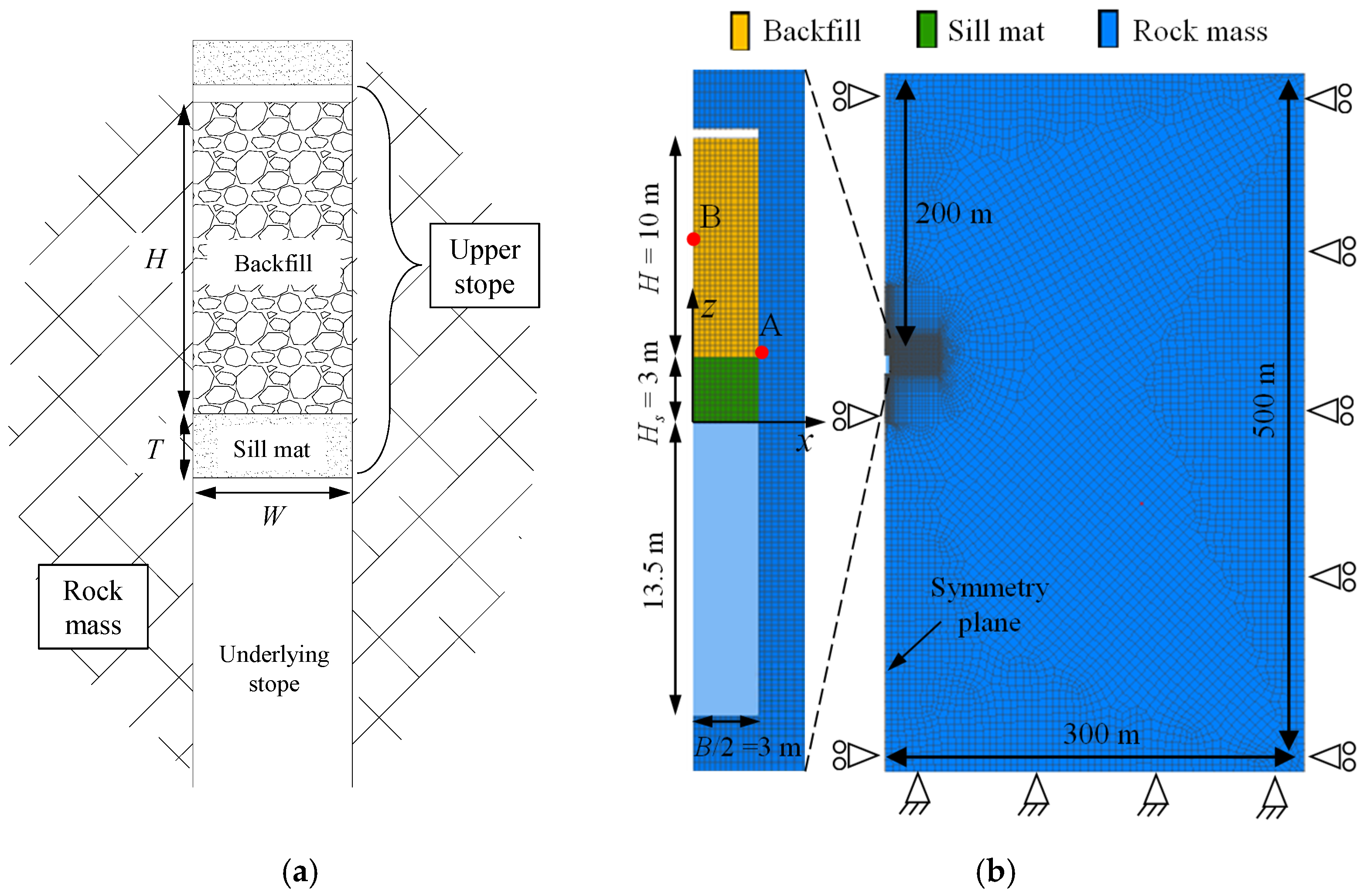
In underhand cut-and-fill mining, uncemented or lightly cemented backfill is used to fill the mined-out upper stope overlying a sill mat. During the extraction of underlying stope, the sill mat will act as an artificial roof, which makes the stress distribution within the overlying backfilled stope significant for its stability. Sobhi and Li [11] analyzed this problem with PLAXIS2D only using the Mohr–Coulomb constitutive model to simulate the backfilled stope. The compressibility of backfill under the rock wall closure associated underlying extraction was thus not properly considered by Sobhi and Li [11]. In this section, the problem of a backfilled stope overlying a sill mat at different mine depths D of 200 and 1000 m are numerically investigated with FLAC3D. Emphasis is placed on the comparisons between numerical results predicted by applying the Mohr–Coulomb and Soft Soil models. Figure 10 shows a physical model and a plane strain numerical model (D = 200 m) of the problem. The symmetry plane (x = 0) is taken into account by considering half of the model. The excavations have a width B of 6 m. The overlying stope has a height H of 10 m and is filled with uncemented backfill. A gap of 0.5 m is left on the top of the backfill to represent the poor contact between fill and stope roof. The sill mat has a height Hs of 3 m, while the underlying stope is 13.5 m in height. The domain size of the numerical model is a distance from the origin to the boundaries of the model. Based on the sensitivity analyses, the numerical model is constructed with the optimal domain and mesh sizes of 300 and 0.25 m.
The rock mass and sill mat obey the Mohr–Coulomb model while the overlying backfill is modeled with different constitutive models. The rock mass is characterized by unit weight γR = 27 kN/m3, Young’s modulus ER = 42 GPa, Poisson’s ratio νR = 0.25, cohesion cR = 9.4 MPa, friction angle ϕR = 38°, and dilation angle ψR = 0°. The sill mat is characterized by unit weight γs = 20 kN/m3, Young’s modulus Es = 1.5 GPa, Poisson’s ratio νs = 0.3, cohesion cs = 5 MPa, friction angle ϕs = 35°, and dilation angle ψs = 0°. Table 3 provides the material parameters for the overlying uncemented backfill in which the same parameters are applied in the Mohr–Coulomb and Soft Soil models, where possible. The shear strength parameters (i.e., ci and ϕi) of fill–rock interfaces are considered equal to those of backfill by assuming rough rock walls.
In the numerical model, the displacement along the third direction (y-axis) is constrained to simulate a two-dimensional plane strain condition. The top boundary of the numerical model is set free to simulate the ground surface while normal displacement is restricted on the lateral boundaries. For the bottom boundary, the displacements are constrained in all directions. Numerical simulations are conducted at mine depths D of 200 and 1000 m respectively. The lateral earth pressure coefficient Kr = 2 is employed by considering the typical stress regime of the Canadian Shield [51]. In numerical simulations, the overlying stope is excavated after obtaining the initial equilibrium state. The displacement is then reset to zero and overlying stope is sequentially backfilled with 1 m per layer. This is followed by excavating the underlying stope in one step to expose the sill mat. Figure 11 shows the displacement distributions in the numerical model at each step as references with the Soft Soil model at a mine depth of 200 m.
Figure 12 shows the iso-contours of bulk modulus in the overlying backfill after placement by applying different constitutive models. In the figure, one sees the bulk modulus of the Mohr–Coulomb model is 250 MPa and is a constant independent on the stope height. The bulk modulus of the Soft Soil model around the middle height of the stope is around 250 MPa, but its value moderately increases along the height of the backfilled stope, because the elastic modulus of the Soft Soil model is mean stress dependent, as given by Equation (17).
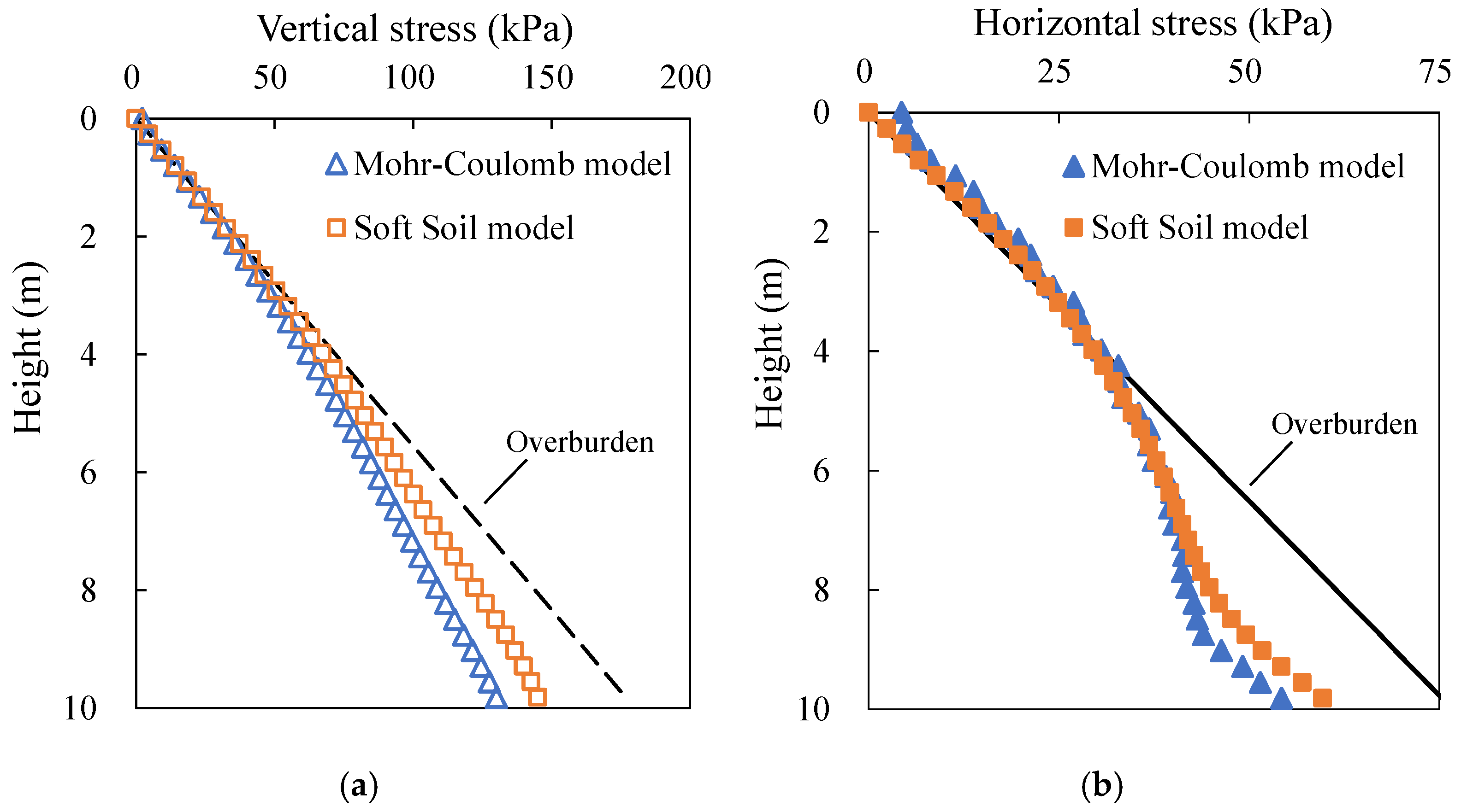
Figure 13 illustrates the variation of the vertical and horizontal stresses along the vertical central line (VCL) of the overlying backfill before the excavation of underlying stope. Results shown in Figure 13 are independent on different mine depths because the backfill is placed after the rock wall displacement (i.e., delayed placement). In the figure, one sees that both the vertical and horizontal stresses increase smoothly along the stope height while the arching effect is evident by comparing with the overburden stresses. The stress distributions in the backfilled stope prior to the underlying excavation by applying the Mohr–Coulomb and Soft Soil models are almost identical. At the lower part of the stope, the stress state of the Soft Soil model is slightly larger than that of the Mohr–Coulomb model. The results shown in Figure 13 agree well with the results reported by Sobhi and Li [11].
Figure 14 shows the variation of vertical and horizontal stresses along the VCL of overlying backfill after excavating the underlying stope at a mine depth D = 200 m. Under the influence of rock wall closure associated with the underlying extraction, the vertical and horizontal stresses in the overlying backfill increase compared to the results shown in Figure 13. However, the vertical and horizontal stresses of the Soft Soil model are smaller than those of the Mohr–Coulomb model below the stope height of 2 m. The value of vertical stress at the bottom of overlying backfill is 256 kPa for the Mohr–Coulomb model and is 169 kPa for the Soft Soil model. The different results of two constitutive models are explained as that the Soft Soil model simulates plastic volumetric strain of backfill under the compression from rock walls. The backfill needs to be compacted with certain amount of compressive strain before it can sustain large compressive stress. This feature is not captured by the Mohr–Coulomb model, which can thus overestimate the stress state in the overlying stope when the rock wall closure is small at a shallow mine depth. Since the stability of sill mat largely depends on the stresses within the overlying backfill, using the Mohr–Coulomb model may further cause an inaccurate estimation on the required strength of sill mat.
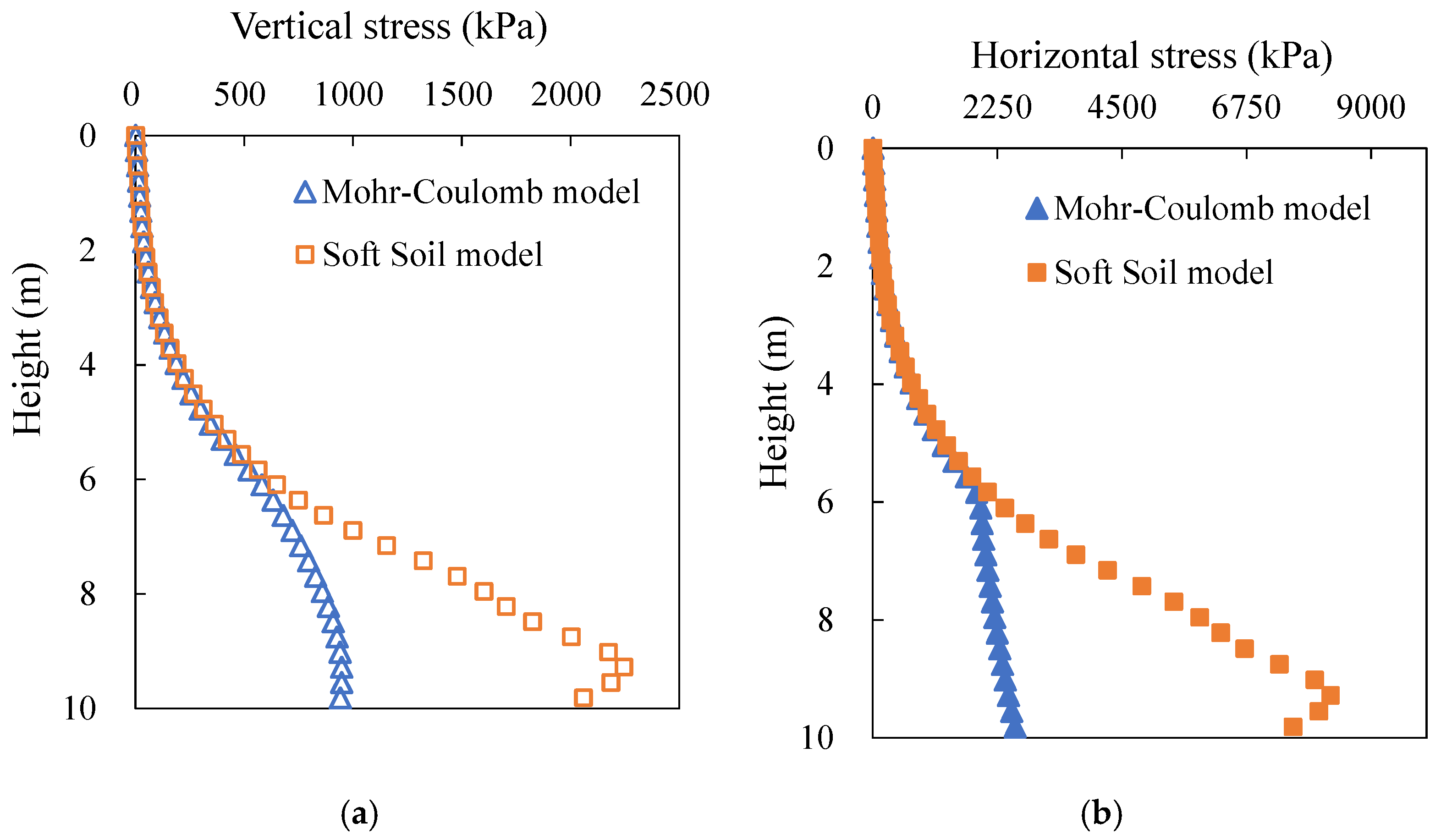
Figure 15 shows the variations of vertical and horizontal stresses along the VCL of overlying backfill after the excavation of underlying stope at a mine depth D = 1000 m. As the mine depth increases from 200 to 1000 m, the rock wall closure associated with underlying excavation becomes larger which increases the vertical and horizontal stresses within the overlying backfill. The stress distribution predicted by the Soft Soil model is similar to that of the Mohr–Coulomb model above the stope height of 6 m as shown in Figure 15. However, the stresses of the Soft Soil model rapidly increase as the stope height increases. At the bottom of overlying backfill, the vertical and horizontal stresses of the Soft Soil model reach 2.2 and 7.5 MPa, which are significantly larger than the values of 0.9 and 2.5 MPa as predicted by the Mohr–Coulomb model. The different results of two constitutive models shown in Figure 15 are attributed to that the Soft Soil model accounts the volumetric hardening and pressure-dependent behavior of backfill. With a significant rock wall closure at a large mine depth, the mining backfill demonstrates large volumetric plastic strain, during which it becomes harder with a large elastic modulus, resulting in an increase in stresses generated by rock wall closure. The Mohr–Coulomb model does not simulate the volumetric hardening of backfill, which, thus, underestimates the stresses in backfilled stopes when the walls convergence is significant at a large mine depth.
Numerical simulations have shown that the Mohr–Coulomb and the Soft Soil models predict similar stress distributions in an isolated backfilled stope when the rock wall closure is absent. However, the stresses within backfill simulated with two constitutive models can be different when closure of surround rock walls is applied. In this condition, the commonly used Mohr–Coulomb model can under- or overestimate the stresses due to the neglect of volumetric yield and pressure-dependent behavior of backfill. The Soft Soil model is deemed more applicable to simulating uncemented or lightly cemented backfill when its compressibility or closure resistance is a dominant factor.
5. Discussion
By comparing the numerical results against the experimental results of one-dimensional consolidation and consolidated drained triaxial compression tests, the Soft Soil model is identified as capable of describing the compressibility of mining backfill. Nonetheless, the Soft Soil model should not be applied for backfill with a very large cohesion. This is partially because that its elliptical yield surface crosses the p-axis at a value of c∙cotϕ on the left side and has an apex on the critical state line as shown in Figure 3b. It implies that the lower bond of preconsolidation pressure in the Soft Soil model is determined by the value of cohesion. When a large cohesion is applied, the backfill modeled with the Soft Soil model is over-consolidated with a significant preconsolidation pressure, which can be unrealistic in some conditions. Another reason is that the slope of the critical state line (Equation (15)) in the Soft Soil model is calculated based on the flow rule of the modified Cam-Clay model, which considers a nil cohesion [42,44].Therefore, the Soft Soil model is deemed applicable to modeling the uncemented or lightly cemented backfill with a small (or nil) cohesion value.
For cemented backfill, cementation increases its primary stiffness at low stress condition by binding together fill particles. Experimental results show that the cement bond can yield as the applied stress increases after which the mechanical behavior of cemented backfill approaches an uncemented condition [26,52]. The results in Figure 6c show that the effect of cementation on fill stiffness at low stress levels can be pseudo-simulated using an over-consolidated state in the Soft Soil model. However, one should note that the mechanisms of cementation and overconsolidation are different. More effort is needed to investigate the effect of cement content and curing time on the compressibility of mining backfill and incorporate it in a constitutive model [52,53,54].
In numerical simulations, the Poisson’s ratio of backfill relates to the friction angle as ν = (1 − sinϕ)/(2 − sinϕ), which is based on a unique value of at-rest earth pressure coefficient K0 [49,50]. Such equation is practical in numerical modeling with an elastoplastic model. Previous studies have proposed several forms of empirical equation to define the relationship between ν and ϕ [55,56]. More works are needed to investigate this aspect based on experimental results. Meanwhile, since the stress–strain curve of soil-like material is highly nonlinear, how to determine the Poisson’s ratio of backfill based on the experimental results for numerical modeling is a problem, and needs to be studied in future works.
The Soft Soil model postulates a perfectly plastic behavior when the stress state reaches the Mohr–Coulomb yield line. The post-peak behavior of backfill is affected by the cement content and confining pressure level [27,29]. Experimental results show that mining backfill with large cement content demonstrates strain softening under small confining pressures at the post-peak stage. The large confining pressure can also result in a strain hardening behavior of mining backfill. The post-peak behavior of backfill is not analyzed in this study.
This study focusses on modeling the compressibility of backfill in the long-term condition while the pore water pressure is not considered. More effort is thus necessary to evaluate the hydraulic conductivity and the effects of pore water pressure and drainage condition on the compressibility of backfill in the short-term condition [57,58,59].
The simulations of a backfilled stope overlying a sill mat indicate the applicability of Soft Soil model and the significance of modeling fill compressibility. The commonly used Mohr–Coulomb model tends to under- or overestimate the stress states in a backfilled stope when the walls closure is applied due to the poor description of the fill compressibility. Although the capability of the Soft Soil model has been tested against some consolidation and triaxial tests, field measurements are still needed when available to make further verifications.
6. Conclusions
The Mohr–Coulomb elasto-plastic, double-yield, and Soft Soil constitutive models are recalled and evaluated for the applicability to describing the compressibility of mining backfill. Numerical results with different constitutive models in FLAC3D are compared with one-dimensional consolidation and consolidated drained triaxial compression tests made on lowly cemented backfill available in the literature. Part of the experimental results is used to calibrate some model parameters and the calibrated models are applied to predict the other part of the test results. Based on the comparisons, the Soft Soil model shows the satisfactory description of the experimental results while its prediction is also quite good. The prevalently used Mohr–Coulomb model demonstrates poor correlations with the experimental results due to the neglect of volumetric yield and pressure-dependent behavior of backfill. The double-yield model accurately describes the experimental results based on the calibration, but its predictive capability is limited when the test results are insufficient.
The comparisons between Soft Soil and Mohr–Coulomb models in simulating a backfilled stope overlying a sill mat at different mine depths show similar stress distributions when rock wall closure is absent. However, when the rock wall closure associated with the underlying extraction is applied, application of the Soft Soil model shows that the Mohr–Coulomb model tends to overestimate the stresses in backfill at a shallow mine depth and underestimate the stresses at a large mine depth due to the poor description of the fill compressibility. The Soft Soil model is recommended to describe the compressibility of uncemented or lightly cemented backfill with small cohesions under external compressions associated with rock wall closure.
Author Contributions
R.W.: conceptualization, numerical modeling, analysis, literature, writing, and editing of the original draft. F.Z.: editing of the original draft. L.L.: project administration, methodology, supervision, editing of the original draft. All authors have read and agreed to the published version of the manuscript.
Funding
This work was financially supported by the Natural Sciences, and Engineering Research Council of Canada (RGPIN-2018-06902), Mitacs Elevate Postdoctoral Fellowship (IT12569 and IT12570), China Scholarship Council (201706420059), and industrial partners of the Research Institute on Mines and the Environment (RIME UQAT-Polytechnique; http://rime-irme.ca/ accessed on 24 November 2021). The authors are grateful for their support.
Institutional Review Board Statement
Not applicable.
Informed Consent Statement
Not applicable.
Data Availability Statement
Data are contained within the article.
Acknowledgments
The authors acknowledge financial support from the Natural Sciences and Engineering Research Council of Canada, Mitacs Elevate Postdoctoral Fellowship, China Scholarship Council, and industrial partners of RIME UQAT-Polytechnique.
Conflicts of Interest
The authors declare no conflict of interest.
List of Symbols
| a | radius of the hole |
| B | width |
| c | cohesion |
| ci | interface cohesion |
| cR | cohesion of rock mass |
| cs | cohesion of sill mat |
| D | mine depth |
| E | Young’s modulus |
| eini | initial value of void ratio |
| ER | Young’s modulus of rock mass |
| Es | Young’s modulus of sill mat |
| G | shear modulus |
| Gmax | upper limit of shear modulus |
| H | height |
| Hs | height of sill mat |
| K | bulk modulus |
| K0 | coefficient of earth pressure at-rest |
| Kmax | upper limit of bulk modulus |
| Kr | lateral earth pressure coefficient |
| Ms | slope of critical state line |
| n | porosity |
| p | mean stress |
| p0 | reference mean stress |
| pc | cap pressure |
| P0 | isotropic in-situ stress |
| Pin | internal pressure |
| q | deviatoric stress |
| R | constant |
| R0 | radius of yield zone around hole |
| T | tensile strength |
| εq | deviatoric strain |
| εv | volumetric strain |
| plastic volumetric strain | |
| reference volumetric strain on normal consolidation line | |
| reference volumetric swelling line | |
| εx, εy, εz | components of normal strain |
| γxy, γyz, γxz | components of shear strain |
| σ | normal stress |
| σ1 | major principal stress |
| σ2 | intermediate principal stress |
| σ3 | minor principal stress |
| σr | radial stress |
| σθ | tangential stress |
| σz | normal stress along third direction |
| σre | radial stress at the elastic-plastic interface |
| σx, σy, σz | components of normal stress |
| , , | normal stress components of in-situ stress field |
| τ | shear strength |
| τrθ, τθz, τzr | shear stresses around cylinder hole |
| τxy, τyz, τxz | components of shear stress |
| , , , | shear stress components of in-situ stress field |
| r, θ | cylindrical coordinates |
| U, V, W | components of displacement |
| ν | Poisson’s ratio |
| νR | Poisson’s ratio of rock mass |
| νs | Poisson’s ratio of sill mat |
| ϕ | friction angle |
| ϕi | interface friction angle |
| ϕR | friction angle of rock mass |
| ϕs | friction angle of sill mat |
| ρ | density |
| ψ | dilation angle |
| ψR | dilation angle of rock mass |
| ψs | dilation angle of sill mat |
| λ* | slope of normal consolidation line |
| κ* | slope of swelling line |
| θl | lode angle |
| γ | unit weight |
| γR | unit weight of rock mass |
| γs | unit weight of sill mat |
Appendix A. Validation of FLAC3D against Analytical Solutions of Stresses and Displacements around a Cylinder Hole in the Linearly Elastic Material
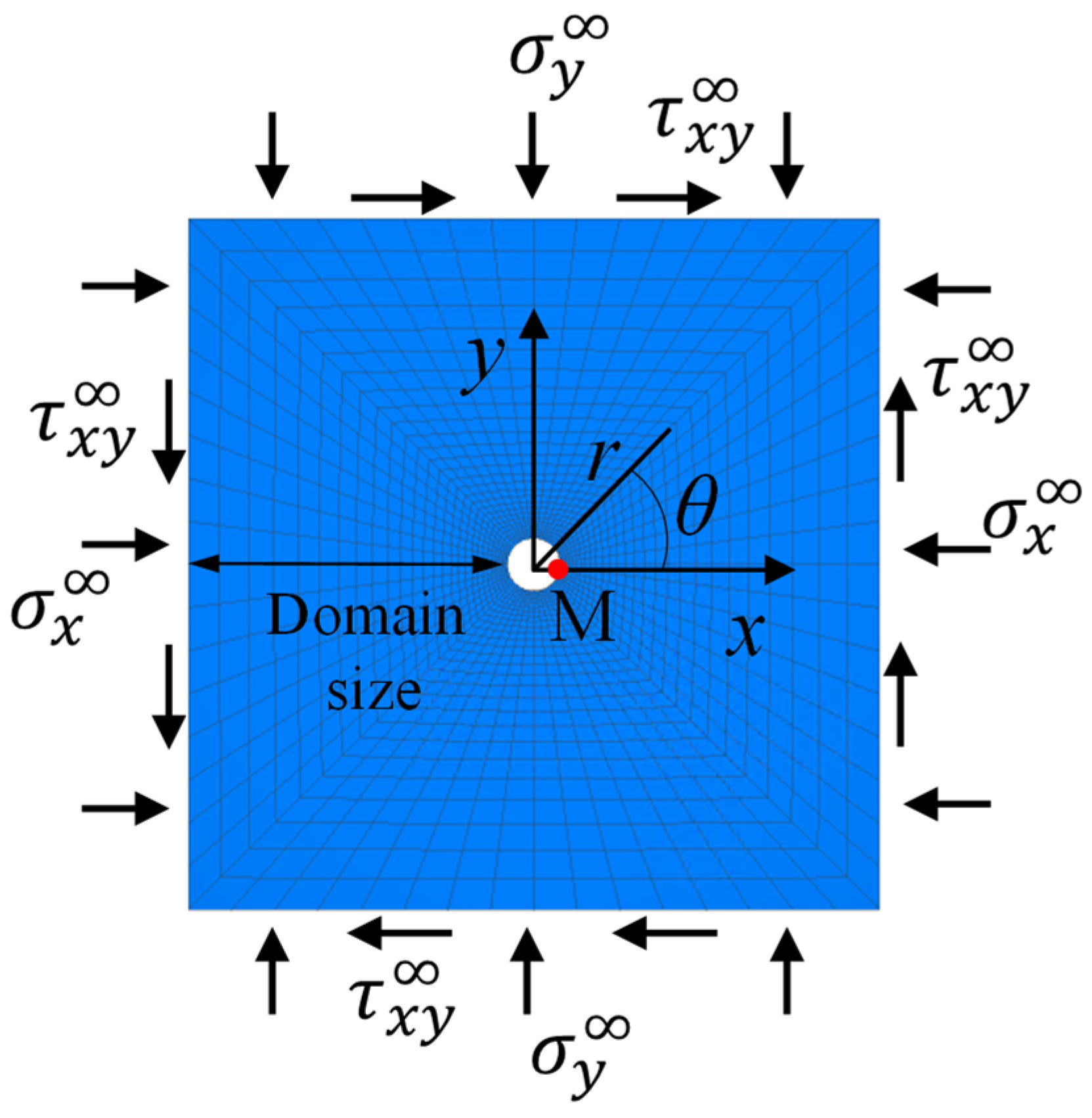
FLAC3D can be validated against analytical solutions of stresses and displacements around an infinite cylinder hole in the infinite linearly elastic material. The problem can be analyzed in a plane strain condition. The physical model of this problem is shown in Figure A1. The origin locates at the central point of the model. In the figure, a is the radius of the hole. Domain size is the distance from the hole to the model boundary. r and θ are the cylindrical coordinates. The model is characterized by Young’s modulus E and Poisson’s ratio ν.
Figure A1.
Physical plane strain model of a cylinder hole in an infinite linearly elastic material.

When the infinite hole is subject to a stress field composed of , , , , , , the analytical solutions for stresses around the hole are given as [60,61]:
where σr is the radial stress; σθ is the tangential stress; σz is the normal stress along third direction (z-axis); τrθ, τθz, and τzr are the shear stresses around infinite cylinder hole based on cylindrical coordinates.
The analytical solutions for displacements around the infinite cylinder hole were given by Li [62], as follows:
where U, V, and W are the components of displacement in the directions of r, θ, and z (third direction), respectively.
Figure A2 shows the corresponding plane strain numerical model built with FLAC3D. In the numerical model, hole radius a = 1 m, E = 10 GPa, ν = 0.25. The applied stress components include = 15 MPa, = 10 MPa, and = 3 MPa. The displacement along the third direction (z-axis) is restricted. In order to ensure stable numerical results, the domain size and mesh size of the numerical model need to be determined based on the sensitivity analyses.
Figure A2.
Plane strain numerical model of a cylinder hole in an infinite linearly elastic material built with FLAC3D.
Figure A2.
Plane strain numerical model of a cylinder hole in an infinite linearly elastic material built with FLAC3D.

The numerical results of radial displacement and tangential stress are obtained at point M in Figure A2. Figure A3 shows the variations of radial displacement and tangential stress at point M as functions of the domain size. The variation of numerical results reduces as the domain size increases from 1 to 20 m, and become stable when the domain size is larger than 10 m. Therefore, the optimal domain size is determined as 12 m that is 6 times the size of the hole.
Figure A3.
Variations of (a) radial displacement and (b) tangential stress at point M as functions of domain size.
Figure A3.
Variations of (a) radial displacement and (b) tangential stress at point M as functions of domain size.

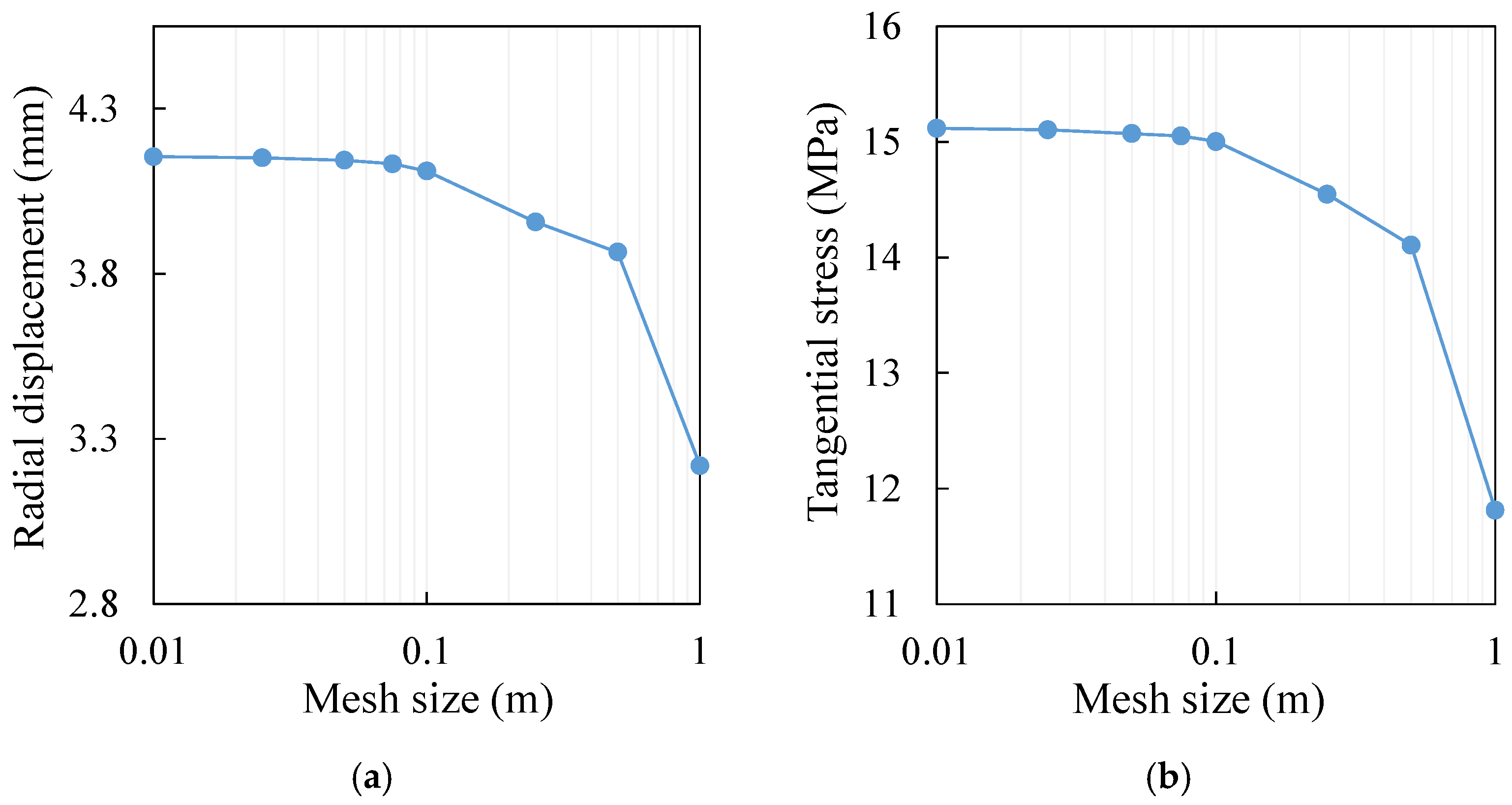
Figure A4 shows the variations of radial displacement and tangential stress at point M as functions of mesh size. The mesh size ranges from 1 to 0.01 m. The numerical results become stable when the mesh size is smaller than 0.1 m. Further reduction of the mesh size will not greatly change the results. Therefore, the optimal mesh size is determined as 0.05 m to ensure stable results.
Figure A4.
Variations of (a) radial displacement and (b) tangential stress at point M as functions of mesh size.
Figure A4.
Variations of (a) radial displacement and (b) tangential stress at point M as functions of mesh size.

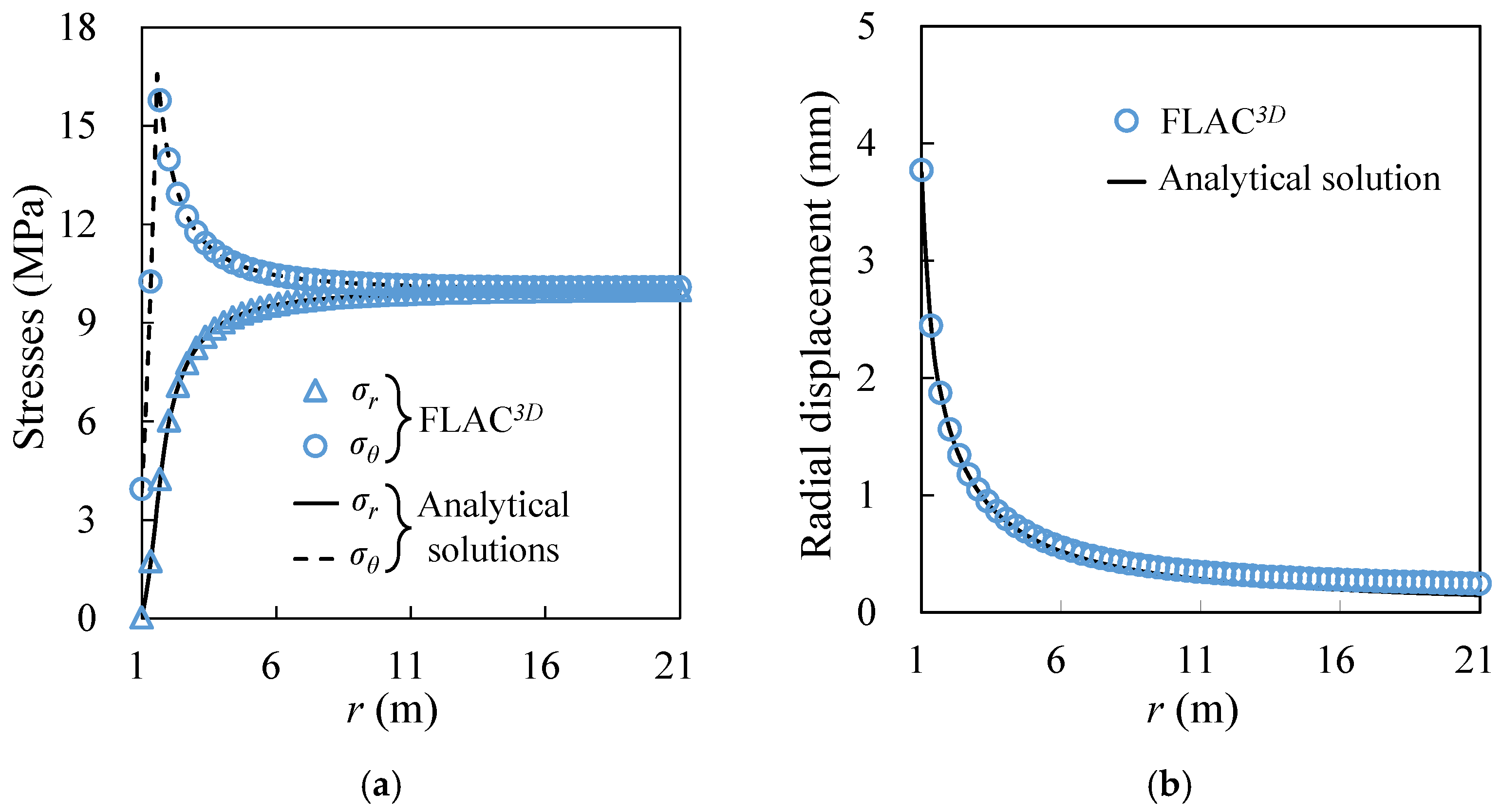
Numerical simulations are then conducted by using the optimal domain and mesh sizes. Figure A5 shows the comparisons between the numerical results of σr, σθ, τrθ, U, V long x-axis with the analytical solutions. The good correlations between the numerical and analytical results validate the FLAC3D.
Figure A5.
Comparisons between the numerical results and the analytical results of (a) σr, (b) σθ, (c) τrθ, (d) V, (e) U long x-axis around a cylinder hole in the linearly elastic material.
Figure A5.
Comparisons between the numerical results and the analytical results of (a) σr, (b) σθ, (c) τrθ, (d) V, (e) U long x-axis around a cylinder hole in the linearly elastic material.

Appendix B. Validation of FLAC3D against Analytical Solutions of Stresses and Displacements around a Cylinder Hole in the Mohr–Coulomb Material
FLAC3D can be further validated against analytical solutions of stresses and displacements around an infinite cylinder hole in the infinite Mohr–Coulomb (MC) material. Figure A6 shows the plane strain physical model of the problem subject to the isotropic in-situ stress P0. The origin is on the central point of the hole. Due to axial symmetry, only one-quarter of the model is considered. In Figure A6, a is the radius of the hole. The model is characterized by Young’s modulus E, Poisson’s ratio ν, cohesion c, friction angle ϕ, and dilation angle ψ.
Figure A6.
Physical plane strain model of a cylinder hole in an infinite MC material.

According to Salencon’s analytical solutions [63], the radius of yield zone R0 around the cylinder hole can be calculated as:
where Pin is the internal pressure; qMC = 2c·tan (45° + ϕ/2); Kp = (1 + sinϕ)/(1 − sinϕ).
The radial stress σr, tangential stress σθ, and radial displacement U in the elastic zone are given as:
where σre is the radial stress at the elastic-plastic interface and is given as:
The stresses and radial displacement in the plastic zone are given as:
where Kψ = (1 + sinψ)/(1 − sinψ).
Figure A7 shows the plane strain numerical model built with FLAC3D. In the numerical model, hole radius a = 1 m, P0 = 10 MPa. The MC material is characterized by E = 10 GPa, ν = 0.25, c = 1 MPa, ϕ = 35°, ψ = 0°. The displacement along the third direction (z-axis) is restricted. Normal displacement on the left boundary and the bottom are prohibited to simulate symmetric planes. Sensitivity analyses are then performed to determine optimal domain and mesh sizes to ensure stable numerical results.
Figure A7.
Plane strain numerical model of a cylinder hole in an infinite MC material built with FLAC3D.
Figure A7.
Plane strain numerical model of a cylinder hole in an infinite MC material built with FLAC3D.

The numerical results of radial displacement and tangential stress are obtained at point M in Figure A7. Figure A8 shows the variations of radial displacement and tangential stress at point M as functions of domain size ranging from 1 to 30 m. The numerical results become stable when the domain size is larger than 12 m. To be conservative, the optimal domain size is determined as 20 m.
Figure A8.
Variations of (a) radial displacement and (b) tangential stress at point M as functions of domain size.
Figure A8.
Variations of (a) radial displacement and (b) tangential stress at point M as functions of domain size.

Figure A9 shows the variations of radial displacement and tangential stress at point M as functions of mesh size. As the mesh size reduces from 1 to 0.005 m, the variation of numerical results decreases. The numerical results become stable when the mesh size reduces to 0.03 mm. Further reduction of the mesh size will not greatly affect the results. Therefore, the optimal mesh size is determined as 0.02 m to ensure stable results.
Figure A9.
Variations of (a) radial displacement and (b) tangential stress at point M as functions of mesh size.
Figure A9.
Variations of (a) radial displacement and (b) tangential stress at point M as functions of mesh size.

The optimal domain and mesh sizes are then used to conduct numerical simulations of the problem. Figure A10 shows the comparisons between the numerical results of stresses and radial displacement long x-axis with the analytical solutions. The good agreements between the numerical and analytical results indicate that the FLAC3D is validated.
Figure A10.
Comparisons between the numerical results and the analytical results of (a) σr and σθ, (b) U along x-axis around a cylinder hole in the MC material.
Figure A10.
Comparisons between the numerical results and the analytical results of (a) σr and σθ, (b) U along x-axis around a cylinder hole in the MC material.

Appendix C. Sensitivity Analyses of Domain and Mesh Sizes in the Numerical Simulations
Sensitivity analyses are conducted to determine the optimal mesh size for the numerical models of consolidation and triaxial tests in this study. For the numerical model of a backfilled stope overlying a sill mat, both optimal domain and mesh sizes are determined based on the sensitivity analyses.
For the one-dimensional consolidation simulation, the physical and numerical models are illustrated in Figure 4 and Figure 5. The material parameters are provided in Table 1. Figure A11 shows the variation of compressive strain under an applied stress of 500 kPa with different constitutive models as a function of the mesh size. The values of mesh sizes vary between 20 and 2 mm. The numerical results are considered stable when the mesh size is smaller than 5 mm.
Figure A11.
Variation of compressive strain under an applied stress of 500 kPa in one-dimensional consolidation simulations as functions of the mesh size.
Figure A11.
Variation of compressive strain under an applied stress of 500 kPa in one-dimensional consolidation simulations as functions of the mesh size.

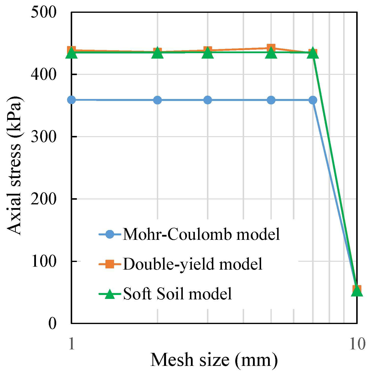
For the numerical simulations of consolidated drained triaxial compression tests, the physical and numerical models are shown in Figure 7 and Figure 8, while the material parameters are provided in Table 2. Figure A12 shows the variation of axial stress under an axial strain of 5% and a confining pressure of 200 kPa with different constitutive models as functions of the mesh size. The values of the mesh sizes range from 10 to 1 mm. The numerical results are considered stable when the mesh size reduces to 3 mm.
Figure A12.
Variation of axial stress under an axial strain of 5% and a confining pressure of 200 kPa in triaxial compression simulations as functions of the mesh size.
Figure A12.
Variation of axial stress under an axial strain of 5% and a confining pressure of 200 kPa in triaxial compression simulations as functions of the mesh size.

For the numerical model of a backfilled stope overlying a sill mat shown in Figure 10b, Mohr–Coulomb model is applied for backfill to conduct the sensitivity analyses at a mine depth of 1000 m. The material parameters are provided in Table 3. In the sensitivity analyses, two indicators are analyzed for different domains and mesh sizes. One is the total displacement of surrounding rock mass at Point A in Figure 10b (one corner of sill mat) after extracting the overlying stope. The other indicator is the horizontal stress after excavating the underlying stope at Point B in Figure 10b, which is at the middle height on the VCL of backfill. Figure A13 shows the variation of total displacement at Point A and horizontal stress at Point B as functions of domain sizes ranging from 35 to 550 m. The numerical results become stable when the domain size is larger than 200 m.
Figure A13.
Variation of (a) total displacement at Point A after extracting the overlying stope and (b) vertical stress at Point B after excavating the underlying stope as functions of domain size.
Figure A13.
Variation of (a) total displacement at Point A after extracting the overlying stope and (b) vertical stress at Point B after excavating the underlying stope as functions of domain size.

Figure A14 shows the variation of total displacement at Point A and horizontal stress at Point B as functions of the mesh size, which ranges from 5 to 0.1 m. The numerical results become stable when the mesh size reduces to 0.5 m.
Figure A14.
Variation of (a) total displacement at Point A after extracting the overlying stope and (b) horizontal stress at Point B after excavating the underlying stope as functions of the mesh size.
Figure A14.
Variation of (a) total displacement at Point A after extracting the overlying stope and (b) horizontal stress at Point B after excavating the underlying stope as functions of the mesh size.

References
- Hassani, F.; Archibald, J. Mine Backfill; Canadian Institute of Mine, Metallurgy and Petroleum: Montreal, QC, Canada, 1998. [Google Scholar]
- Benzaazoua, M.; Bussière, B.; Demers, I.; Aubertin, M.; Fried, É.; Blier, A. Integrated mine tailings management by combining environmental desulphurization and cemented paste backfill: Application to mine Doyon, Quebec, Canada. Min. Eng. 2008, 21, 330–340. [Google Scholar] [CrossRef]
- Stephan, G. Cut-and-fill mining. In SME Mining Engineering Handbook, 3rd ed.; Society for Mining, Metallurgy and Exploration: Littleton, CO, USA, 2011; pp. 1365–1373. [Google Scholar]
- Kortnik, J. Green mining–use of hydraulic backfill in the Velenje Coal Mine. In Proceedings of the 13th International Symposium on Mining with Backfill, Katowice, Poland, 25–28 May 2021; pp. 422–432. [Google Scholar]
- Potvin, Y.; Thomas, E.; Fourie, A. Handbook on Mine Fill; Australian Centre for Geomechanics: Perth, Australia, 2005. [Google Scholar]
- Newman, C.R.; Agioutantis, Z.G. Stress redistribution around single and multiple stope-and-fill operations. In Proceedings of the 52nd US Rock Mechanics/Geomechanics Symposium, Seattle, WA, USA, 17–20 June 2018. [Google Scholar]
- Zhao, T.; Ma, S.; Zhang, Z. Ground control monitoring in backfilled strip mining under the metropolitan district: Case study. Int. J. Geomech. 2018, 18, 05018003. [Google Scholar] [CrossRef]
- Vasichev, S. Ground control with backfill and caving in deep-level mining of gently dipping ore bodies. In Proceedings of the IOP Conference Series: Earth and Environmental Science, Subsurface Management, Exploration and Mining Technologies, Economics, Geoecology, Novosibirsk, Russia, 24–26 April 2019; p. 012022. [Google Scholar]
- Wang, R.; Zeng, F.; Li, L. Stability analyses of side-exposed backfill considering mine depth and extraction of adjacent stope. Int. J. Rock Mech. Min. Sci. 2021, 142, 104735. [Google Scholar] [CrossRef]
- Falaknaz, N.; Aubertin, M.; Li, L. Numerical investigation of the geomechanical response of adjacent backfilled stopes. Can. Geotech. J. 2015, 52, 1507–1525. [Google Scholar] [CrossRef]
- Sobhi, M.A.; Li, L. Numerical investigation of the stresses in backfilled stopes overlying a sill mat. J. Rock Mech. Geotech. Eng. 2017, 9, 490–501. [Google Scholar] [CrossRef]
- Raffaldi, M.J.; Seymour, J.B.; Richardson, J.; Zahl, E.; Board, M. Cemented paste backfill geomechanics at a narrow-vein underhand cut-and-fill mine. Rock Mech. Rock Eng. 2019, 52, 4925–4940. [Google Scholar] [CrossRef] [PubMed]
- Qi, C.; Fourie, A. Numerical investigation of the stress distribution in backfilled stopes considering creep behaviour of rock mass. Rock Mech. Rock Eng. 2019, 52, 3353–3371. [Google Scholar] [CrossRef]
- Brinkgreve, R.B.J. Selection of soil models and parameters for geotechnical engineering application. In Proceedings of the Geo-Frontiers Congress, Austin, TX, USA, 24–26 January 2005; pp. 69–98. [Google Scholar]
- Helinski, M.; Fahey, M.; Fourie, A. Numerical modeling of cemented mine backfill deposition. J. Geotech. Geoenviron. Eng. 2007, 133, 1308–1319. [Google Scholar] [CrossRef] [Green Version]
- Li, L.; Aubertin, M.; Shirazi, A. Implementation and application of a new elastoplastic model based on a multiaxial criterion to assess the stress state near underground openings. Int. J. Geomech. 2010, 10, 13–21. [Google Scholar] [CrossRef]
- Cui, L.; Fall, M. A coupled thermo–hydro-mechanical–chemical model for underground cemented tailings backfill. Tunn. Undergr. Space Technol. 2015, 50, 396–414. [Google Scholar] [CrossRef]
- Aubertin, M.; Li, L.; Arnoldi, S.; Belem, T.; Bussière, B.; Benzaazoua, M.; Simon, R. Interaction between backfill and rock mass in narrow stopes. In Proceedings of the 12th Panamerican Conference on Soil Mechanics and Geotechnical Engineering and 39th U.S. Rock Mechanics Symposium, Cambridge, MA, USA, 22–26 June 2003; pp. 1157–1164. [Google Scholar]
- Li, L.; Aubertin, M.; Simon, R.; Bussière, B.; Belem, T. Modeling arching effects in narrow backfilled stopes with FLAC. In Proceedings of the 3rd International Symposium on FLAC and FLAC3D Numerical Modelling in Geomechanics, Sudbury, ON, Canada, 22–24 October 2003; pp. 211–219. [Google Scholar]
- Pirapakaran, K.; Sivakugan, N. Arching within hydraulic fill stopes. Geotech. Geol. Eng. 2007, 25, 25–35. [Google Scholar] [CrossRef]
- Emad, M.Z.; Mitri, H.S.; Henning, J.G. Effect of blast vibrations on the stability of cemented rockfill. Int. J. Min. Reclam. Environ. 2012, 26, 233–243. [Google Scholar] [CrossRef]
- Li, L.; Aubertin, M. An improved method to assess the required strength of cemented backfill in underground stopes with an open face. Int. J. Min. Sci. Technol. 2014, 24, 549–558. [Google Scholar] [CrossRef]
- Liu, G.; Li, L.; Yang, X.; Guo, L. Numerical analysis of stress distribution in backfilled stopes considering interfaces between the backfill and rock walls. Int. J. Geomech. 2017, 17, 06016014. [Google Scholar] [CrossRef]
- Pagé, P.; Li, L.; Yang, P.; Simon, R. Numerical investigation of the stability of a base-exposed sill mat made of cemented backfill. Int. J. Rock Mech. Min. Sci. 2019, 114, 195–207. [Google Scholar] [CrossRef]
- Keita, A.M.T.; Jahanbakhshzadeh, A.; Li, L. Numerical analysis of the stability of arched sill mats made of cemented backfill. Int. J. Rock Mech Min. Sci. 2021, 140, 104667. [Google Scholar] [CrossRef]
- Pierce, M.E. Laboratory and Numerical Analysis of the Strength and Deformation Behaviour of Paste Backfill. Master’s Thesis, Queen’s University, Kingston, ON, Canada, 1999. [Google Scholar]
- Belem, T.; Benzaazoua, M.; Bussière, B. Mechanical behaviour of cemented paste backfill. In Proceedings of the 53rd Canadian Geotechnical Conference, Montreal, QC, Canada, 15–18 October 2000; pp. 373–380. [Google Scholar]
- Rankine, R.M. The Geotechnical Characterisation and Stability Analysis of BHP Billiton’s Cannington Mine Paste fill. Ph.D. Thesis, James Cook University, Douglas, Australia, 2004. [Google Scholar]
- Fall, M.; Belem, T.; Samb, S.; Benzaazoua, M. Experimental characterization of the stress–strain behaviour of cemented paste backfill in compression. J. Mater. Sci. 2007, 42, 3914–3922. [Google Scholar] [CrossRef]
- Jafari, M.; Shahsavari, M.; Grabinsky, M. Drained triaxial compressive shear response of cemented paste backfill (CPB). Rock Mech. Rock Eng. 2021, 54, 3309–3325. [Google Scholar] [CrossRef]
- Oliver, P.H.; Landriault, D. The convergence resistance of mine backfills. In Proceedings of the 4th International Symposium on mining with backfill, Montreal, QC, Canada, 2–5 October 1989; pp. 433–436. [Google Scholar]
- Clark, I.H. The cap model for stress path analysis of mine backfill compaction processes. In Proceedings of the 7th International Conference on Computer Methods and Advances in Geomechanics, Cairns, Australia, 6–10 May 1991; pp. 1293–1298. [Google Scholar]
- Fourie, A.B.; Gürtunca, R.G.; De Swardt, G.; Wendland, E. An evaluation of four constitutive models for the simulation of backfill behaviour. In Proceedings of the 5th International Symposium on Mining with Backfill, Johannesburg, South Africa, 7–9 June 1993; pp. 33–38. [Google Scholar]
- Lagger, M.; Henzinger, M.R.; Schubert, W. Numerical investigations on pea gravel using a nonlinear constitutive model. In Proceedings of the ISRM International Symposium-EUROCK, Cappadocia, Turkey, 29–31 August 2016; pp. 521–526. [Google Scholar]
- Labuz, J.F.; Zang, A. Mohr–Coulomb failure criterion. Rock Mech. Rock Eng. 2012, 45, 975–979. [Google Scholar] [CrossRef] [Green Version]
- Mohr, O. Welche Umstände bedingen die Elastizitätsgrenze und den Bruch eines Materials. Zeit. des Ver. Deut. Ing. 1900, 44, 1524–1530. [Google Scholar]
- Coulomb, C.A. Sur une application des règles de mximis et mnimis à qelques poblèmes de satique relatits à l’architecture. Académie R. Des Sci. Mémoires De Mathématique Et De Phys. 1773, 7, 343–382. [Google Scholar]
- Pietruszczak, S. Fundamentals of Plasticity in Geomechanics; CRC Press: Boca Raton, FL, USA, 2010. [Google Scholar]
- Mitchell, R.J.; Wong, B.C. Behaviour of cemented tailings sands. Can. Geotech. J. 1982, 19, 289–295. [Google Scholar] [CrossRef]
- Itasca. FLAC3D—Fast Lagrangian Analysis of Continua in 3 Dimensions; User’s Guide; Version 7.0; Itasca Consulting Group: Minneapolis, MN, USA, 2019. [Google Scholar]
- Antonov, D. Optimization of the Use of Cement in Backfilling Operations. Ph.D. Thesis, École Polytechnique de Montréal, Montréal, QC, Canada, 2005. [Google Scholar]
- Brinkgreve, R.B.J. Geomaterial Models and Numerical Analysis of Softening. Ph.D. Thesis, Delft University of Technology, Delft, The Netherlands, 1996. [Google Scholar]
- Roscoe, K.H.; Schofield, A.N.; Wroth, C.P. On the yielding of soils. Géotechnique 1958, 8, 22–53. [Google Scholar] [CrossRef]
- Burland, J.B. Correspondence on the yielding and dilation of clay. Géotechnique 1965, 15, 211–214. [Google Scholar] [CrossRef]
- Neher, H.; Wehnert, M.; Bonnier, P. An evaluation of soft soil models based on trial embankments. In Proceedings of the 10th International Conference on Computer Methods and Advances in Geomechanics, Tucson, AZ, USA, 7–12 January 2001; pp. 373–379. [Google Scholar]
- Kahlström, M. Plaxis 2D Comparison of Mohr-Coulomb and Soft Soil Material Models. Master’s Thesis, Luleå University of Technology, Luleå, Sweden, 2013. [Google Scholar]
- Canadian Geotechnical Society. Canadian Foundation Engineering Manual; BiTech Publishers Ltd.: Richmond, BC, Canada, 1978. [Google Scholar]
- Bowles, L. Foundation Analysis and Design, 5th ed.; McGraw-hill: New York, NY, USA, 1996. [Google Scholar]
- Duncan, J.M.; Bursey, A. Soil modulus correlations. In Foundation Engineering in the Face of Uncertainty; James, L.W., Kok-Kwang, P., Mohamad, H., Eds.; American Society of Civil Engineers: Reston, VA, USA, 2013; pp. 321–336. [Google Scholar]
- Yang, P.; Li, L.; Aubertin, M. Theoretical and numerical analyses of earth pressure coefficient along the centerline of vertical openings with granular fills. Appl. Sci. 2018, 8, 1721. [Google Scholar] [CrossRef] [Green Version]
- Herget, G. Stresses in Rock; AA Balkema: Rotterdam, The Netherlands, 1988. [Google Scholar]
- Stewart, J.M.; Clark, I.H.; Morris, A.N. Assessment of fill quality as a basis for selecting and developing optimal backfill systems for South African gold mines. In Proceedings of the International Conference on Gold, Johannesburg, South Africa, 15–17 September 1986; pp. 255–270. [Google Scholar]
- Liu, M.D.; Carter, J.P. Virgin compression of structured soils. Géotechnique 1999, 49, 43–57. [Google Scholar] [CrossRef] [Green Version]
- Jafari, M.; Shahsavari, M.; Grabinsky, M. Experimental study of the behavior of cemented paste backfill under high isotropic compression. J. Geotech. Geoenviron. Eng. 2020, 146, 06020019. [Google Scholar] [CrossRef]
- Duncan, J.M.; Williams, G.W.; Sehn, A.L.; Seed, R.B. Estimation earth pressures due to compaction. J. Geotech. Eng. 1991, 117, 1833–1847. [Google Scholar] [CrossRef]
- Yang, P. Investigation of the Geomechanical Behavior of Mine Backfill and Its Interaction with Rock Walls and Barricades. Ph.D. Thesis, École Polytechnique de Montréal, Montréal, QC, Canada, 2016. [Google Scholar]
- Pariseau, W.G. Coupled three-dimensional finite element modeling of mining in wet ground. In Proceedings of the 3rd Canadian Conference on Computer Applications in the Mineral Industry, Montreal, QC, Canada, 22–25 October 1995; pp. 283–292. [Google Scholar]
- Godbout, J.; Bussière, B.; Belem, T. Evolution of cemented paste backfill saturated hydraulic conductivity at early curing time. In Proceedings of the Diamond Jubilee Canadian Geotechnical Conference and the 8th Joint CGS/IAH-CNC Groundwater Conference, Ottawa, ON, Canada, 21–25 October 2007. [Google Scholar]
- Fall, M.; Adrien, D.; Célestin, J.; Pokharel, M.; Touré, M. Saturated hydraulic conductivity of cemented paste backfill. Miner Eng. 2009, 22, 1307–1317. [Google Scholar] [CrossRef]
- Hiramatsu, Y.; Oka, Y. Analysis of stress around a circular shaft or drift excavated in ground in a three dimensional stress state. J. Min. Metall. Inst. Jpn. 1962, 78, 93–98. [Google Scholar]
- Hiramatsu, Y.; Oka, Y. Determination of the stress in rock unaffected by boreholes or drifts, from measured strains or deformations. Int. J. Rock Mech. Min. Sci. Geomech. Abstr. 1968, 5, 337–353. [Google Scholar] [CrossRef]
- Li, L. Étude Expérimentale Du Comportement Hydromécanique D’une Fracture. Ph.D. Thesis, Institut de Physique du Globe de Paris, Université Paris 7, Paris, France, 1997. [Google Scholar]
- Salencon, J. Contraction Quasi-statique d’une cavité à symétrie sphérique ou cylindrique dans un milieu élastoplastique. Ann. Ponts Chaussés 1969, 4, 231–236. [Google Scholar]
Figure 1.
Schematic presentation of the Mohr–Coulomb elasto-plastic model: (a) yield surface in p–q space; (b) stress–strain relationship.
Figure 1.
Schematic presentation of the Mohr–Coulomb elasto-plastic model: (a) yield surface in p–q space; (b) stress–strain relationship.

Figure 2.
Schematic presentation of the double-yield model: (a) yield surface in p–q space; (b) stress–strain relationship.
Figure 2.
Schematic presentation of the double-yield model: (a) yield surface in p–q space; (b) stress–strain relationship.

Figure 3.
Schematic presentation of the Soft Soil model: (a) logarithmic relation between the volumetric strain and mean stress; (b) yield surface in p–q space; (c) stress–strain relationship.
Figure 3.
Schematic presentation of the Soft Soil model: (a) logarithmic relation between the volumetric strain and mean stress; (b) yield surface in p–q space; (c) stress–strain relationship.


Figure 4.
Physical model and stress–strain curve of one-dimensional consolidation tests on Golden Giant paste backfill with a binder content of 3% and a curing time of 28 days conducted by Pierce [26].
Figure 4.
Physical model and stress–strain curve of one-dimensional consolidation tests on Golden Giant paste backfill with a binder content of 3% and a curing time of 28 days conducted by Pierce [26].

Figure 5.
A numerical model of one-dimensional consolidation tests built with FLAC3D.

Figure 6.
Comparisons between the experimental results of one-dimensional consolidation tests reported by Pierce [26] and the numerical results by applying the (a) Mohr–Coulomb; (b) double-yield; and (c) Soft Soil models for backfill with parameters in Table 1.

Figure 7.
Physical model and deviatoric stress–strain curve under different confining pressures of consolidated drained compression triaxial tests on Cannington paste backfill, with a cement content of 2% and a curing time of 28 days performed by Rankine [28].
Figure 7.
Physical model and deviatoric stress–strain curve under different confining pressures of consolidated drained compression triaxial tests on Cannington paste backfill, with a cement content of 2% and a curing time of 28 days performed by Rankine [28].

Figure 8.
A numerical model of consolidated drained triaxial compression tests built with FLAC3D.

Figure 9.
Comparisons between the experimental results (dash lines with points) of consolidated drained triaxial compression tests reported by Rankine [28] and the numerical results (solid lines) under different confining pressures by applying the (a) Mohr–Coulomb; (b) double-yield and (c) Soft Soil models for backfill with parameters in Table 2.

Figure 10.
(a) Physical model and (b) numerical model built with FLAC3Dof an undercut below a sill mat with overlying backfill.
Figure 10.
(a) Physical model and (b) numerical model built with FLAC3Dof an undercut below a sill mat with overlying backfill.

Figure 11.
Distributions of the displacement with the Soft Soil model at a mine depth of 200 m for different simulation steps of (a) excavating the overlying stope; (b) backfilling the mined-out overlying stope; and (c) extracting the underlying stope.
Figure 11.
Distributions of the displacement with the Soft Soil model at a mine depth of 200 m for different simulation steps of (a) excavating the overlying stope; (b) backfilling the mined-out overlying stope; and (c) extracting the underlying stope.

Figure 12.
Distributions of the bulk modulus in overlying backfill after placement simulated with the (a) Mohr–Coulomb and (b) Soft Soil models.
Figure 12.
Distributions of the bulk modulus in overlying backfill after placement simulated with the (a) Mohr–Coulomb and (b) Soft Soil models.

Figure 13.
Variation of the (a) vertical and (b) horizontal stresses along the VCL of overlying backfilled stope before the underlying extraction.
Figure 13.
Variation of the (a) vertical and (b) horizontal stresses along the VCL of overlying backfilled stope before the underlying extraction.

Figure 14.
Variations of the (a) vertical and (b) horizontal stresses along the VCL of overlying backfill after excavating the underlying stope at a mine depth of 200 m.
Figure 14.
Variations of the (a) vertical and (b) horizontal stresses along the VCL of overlying backfill after excavating the underlying stope at a mine depth of 200 m.

Figure 15.
Variation of the (a) vertical and (b) horizontal stresses along the VCL of overlying backfill after excavating the underlying stope at a mine depth of 1000 m.
Figure 15.
Variation of the (a) vertical and (b) horizontal stresses along the VCL of overlying backfill after excavating the underlying stope at a mine depth of 1000 m.


Table 1.
Parameters of different constitutive models applied for backfill in numerical simulations of one-dimensional consolidation tests with ρ = 2013 kg/m3, ϕi = 27°, ci = 40 kPa.
Table 1.
Parameters of different constitutive models applied for backfill in numerical simulations of one-dimensional consolidation tests with ρ = 2013 kg/m3, ϕi = 27°, ci = 40 kPa.
| Constitutive Models | Parameters | |||||||||
|---|---|---|---|---|---|---|---|---|---|---|
| Mohr- Coulomb | K (kPa) | G (kPa) | ϕ (°) | c (kPa) | ψ (°) | T (kPa) | ||||
| 5388 | 3141 | 41 | 40 | 0 | 17.6 | |||||
| Double- yield | Kmax (GPa) | Gmax (GPa) | ϕ (°) | c (kPa) | ψ (°) | T (kPa) | R | |||
| 50 | 29.2 | 41 | 40 | 0 | 17.6 | 24.1 | ||||
| Prescribed piecewise-linear function for cap (kPa) hardening in terms of ( , Pc) | ||||||||||
| (0, 0); (0.008, 12); (0.0094, 14.2); (0.0103, 15.5); (0.0119, 30.5); (0.0178, 69.59); (0.0181, 72); (0.0246, 87.5); (0.0273, 92.46); (0.0301, 97.5); (0.0336, 120); (0.0393, 144.71); (0.0449, 169.2); (0.0479, 187); (0.0492, 193.73); (0.0573, 237); (0.0592, 246.89); (0.0611, 257); (0.0631, 285.97); (0.0689, 294.84); (0.0714, 310); (0.0741, 325); (0.0889, 455.85) | ||||||||||
| Soft Soil | ν | ϕ (°) | c (kPa) | ψ (°) | T (kPa) | κ* | λ* | K0 | pc (kPa) | eini |
| 0.26 | 41 | 40 | 0 | 17.6 | 0.0052 | 0.051 | 0.34 | 127 | 0.961 | |
Note: Kmax and Gmax denote the upper limits of the bulk and shear modulus. K and G for the Mohr–Coulomb model, R and piecewise-linear function of pc for the double-yield model, λ*, κ*, and pc for the Soft Soil model are calibrated based on the experimental results.
Table 2.
Parameters of different constitutive models applied for backfill in numerical simulations of the consolidated drained triaxial compression tests with ρ = 2091 kg/m3.
Table 2.
Parameters of different constitutive models applied for backfill in numerical simulations of the consolidated drained triaxial compression tests with ρ = 2091 kg/m3.
| Constitutive Models | Parameters | |||||||||
|---|---|---|---|---|---|---|---|---|---|---|
| Mohr- Coulomb | K (kPa) | G (kPa) | ϕ (°) | c (kPa) | ψ (°) | T (kPa) | ||||
| 2935 | 1203 | 32 | 14.73 | 0 | 21.8 | |||||
| Double- yield | Kmax (GPa) | Gmax (GPa) | ϕ (°) | c (kPa) | ψ (°) | T (kPa) | R | |||
| 50 | 20.5 | 32 | 14.73 | 0 | 21.8 | 2 | ||||
| Prescribed piecewise-linear function for cap (kPa) hardening (, Pc) | ||||||||||
| (0, 0); (0.052, 50); (0.103, 100); (0.155, 150); (0.196, 190); (0.2, 200); (0.218, 250); (0.237, 300); (0.256, 350); (0.274, 400); (0.312, 500); (0.376, 670); (0.383, 690); (0.387, 700) | ||||||||||
| Soft Soil | ν | ϕ (°) | c (kPa) | ψ (°) | T (kPa) | κ* | λ* | K0 | pc (kPa) | eini |
| 0.32 | 32 | 14.73 | 0 | 21.8 | 0.0078 | 0.135 | 0.47 | 50 | 1.05 | |
Note: c and ϕ, K and G for the Mohr–Coulomb model, R and the piecewise-linear function of pc for the double-yield model, λ*, κ*, and pc for the Soft Soil model are calibrated based on the experimental results.
Table 3.
Parameters of the Mohr–Coulomb and Soft Soil models applied for overlying uncemented backfill with unit weight γ = 18 kN/m3.
Table 3.
Parameters of the Mohr–Coulomb and Soft Soil models applied for overlying uncemented backfill with unit weight γ = 18 kN/m3.
| Constitutive Models | Parameters | |||||||||
|---|---|---|---|---|---|---|---|---|---|---|
| Mohr- Coulomb | K (MPa) | G (MPa) | ϕ (°) | c (kPa) | ψ (°) | T (kPa) | ||||
| 250 | 115 | 35 | 0 | 0 | 0 | |||||
| Soft Soil | ν | ϕ (°) | c (kPa) | ψ (°) | κ* ×10−3 | λ* ×10−3 | T (kPa) | K0 | pc (kPa) | eini |
| 0.3 | 35 | 0 | 0 | 0.2 | 1 | 0 | 0.43 | 1 | 0.9 | |
Publisher’s Note: MDPI stays neutral with regard to jurisdictional claims in published maps and institutional affiliations. |
© 2021 by the authors. Licensee MDPI, Basel, Switzerland. This article is an open access article distributed under the terms and conditions of the Creative Commons Attribution (CC BY) license (https://creativecommons.org/licenses/by/4.0/).
Share and Cite
MDPI and ACS Style
Wang, R.; Zeng, F.; Li, L. Applicability of Constitutive Models to Describing the Compressibility of Mining Backfill: A Comparative Study. Processes 2021, 9, 2139. https://0-doi-org.brum.beds.ac.uk/10.3390/pr9122139
AMA Style
Wang R, Zeng F, Li L. Applicability of Constitutive Models to Describing the Compressibility of Mining Backfill: A Comparative Study. Processes. 2021; 9(12):2139. https://0-doi-org.brum.beds.ac.uk/10.3390/pr9122139
Chicago/Turabian StyleWang, Ruofan, Feitao Zeng, and Li Li. 2021. "Applicability of Constitutive Models to Describing the Compressibility of Mining Backfill: A Comparative Study" Processes 9, no. 12: 2139. https://0-doi-org.brum.beds.ac.uk/10.3390/pr9122139
Note that from the first issue of 2016, this journal uses article numbers instead of page numbers. See further details here.