Temperature-Dependent Viscosity Model for Silicone Oil and Its Application in Viscous Dampers

Abstract

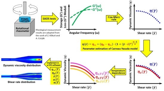
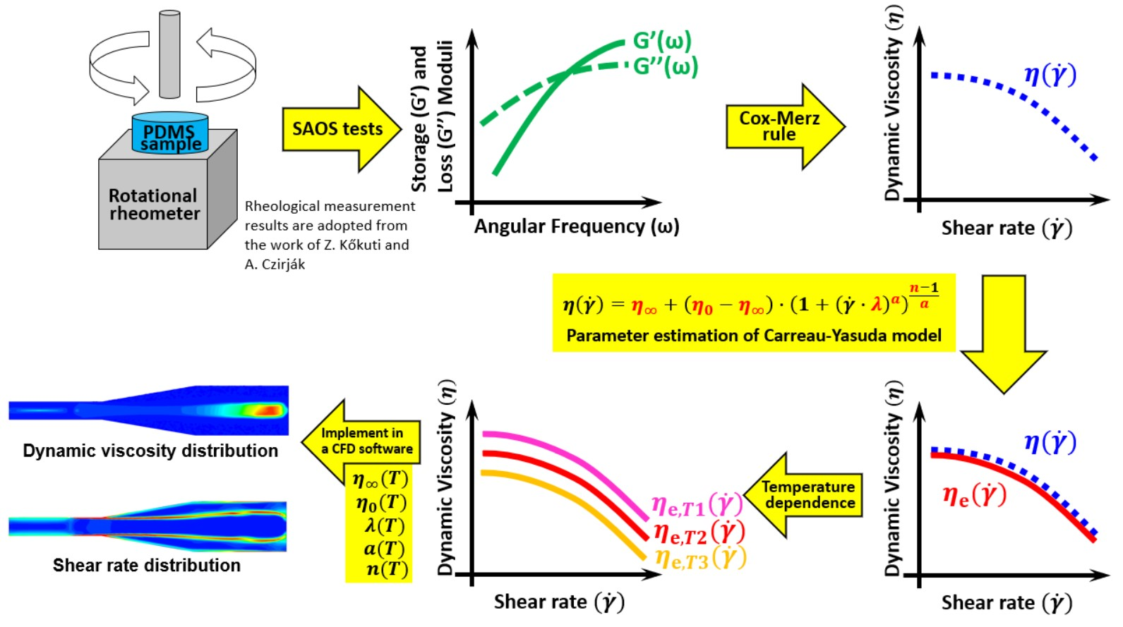
Silicone fluids belong to the group of pseudoplastic non-Newtonian fluids with complex rheological characteristics. They are considered in basic and applied researches and in a wide range of industrial applications due to their favorable physical and thermal properties. One of their specific field of applications in the automotive industry is the working fluid of viscous torsional vibration dampers. For numerical studies in the design and development phase of this damping product, it is essential to have thorough rheological knowledge and mathematical description about the silicone oil viscosity. In the present work, adopted rheological measurement results conducted on polydimethylsiloxane manufactured by Wacker Chemie with initial viscosity of 1000 Pas (AK 1 000 000 STAB silicone oil) are processed. As a result of the parameter identification by nonlinear regression, the temperature-dependent parameter curves of the Carreau–Yasuda non-Newtonian viscosity model are generated. By implementing these parameter sets into a Computational Fluid Dynamics (CFD) software, a temperature- and shear-rate-dependent viscosity model of silicone fluid was tested, using transient flow and thermal simulations on elementary tube geometries in the size range of a real viscous torsional vibration damper’s flow channels and filling chambers. The numerical results of the finite volume method provide information about the developed flow processes, with especial care for the resulted flow pattern, shear rate, viscosity and timing.

1. Introduction

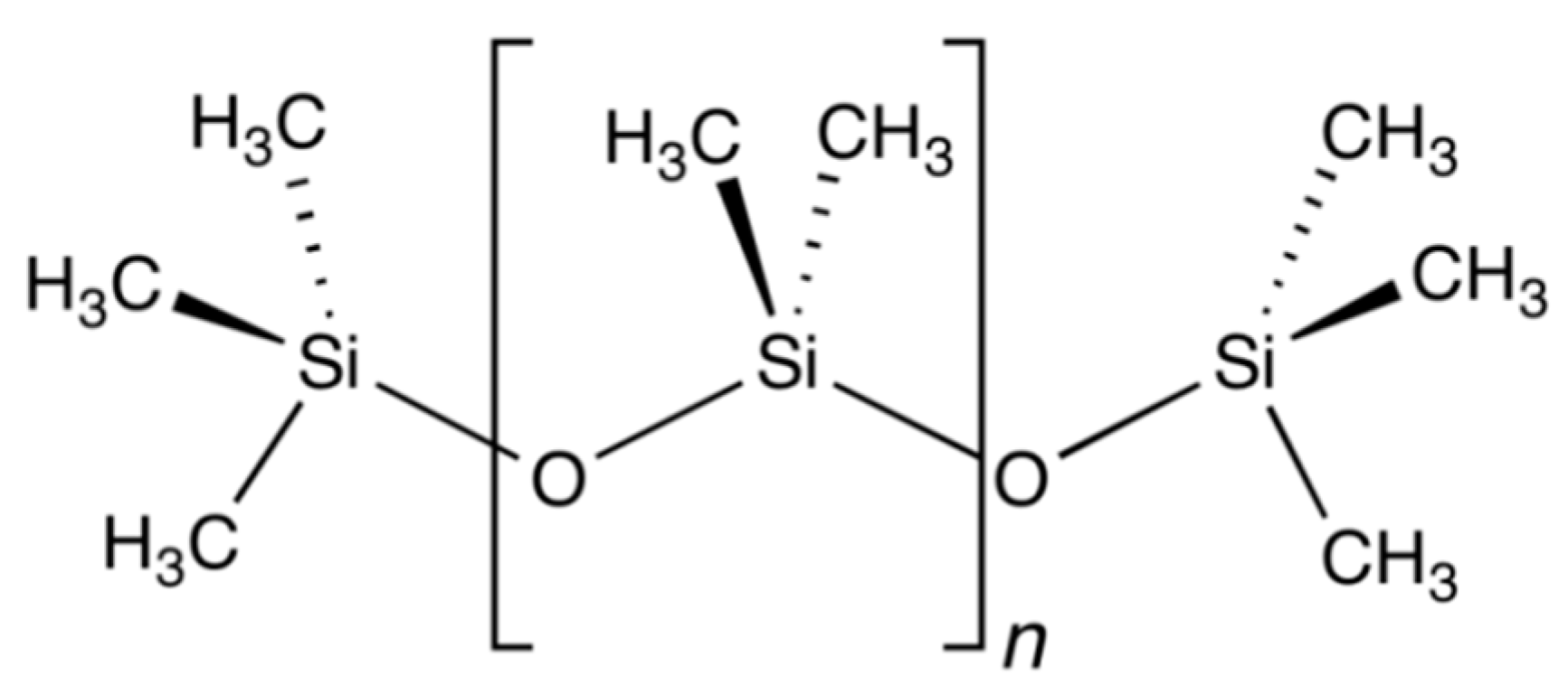
Polydimethylsiloxane (PDMS), or silicone oil, is a type of liquid polymerized siloxane (Si-O) whose molecules contain organic side chains (for instance, CH³ methyl radicals). Its chemical formula can be written as (H₃C)₃[Si(CH₃)₂O]_nSi(CH₃)₃, where n is the number of repeating monomer units, and the higher this number, the higher the viscosity of the sample [1]. The described molecular chain is shown in Figure 1.

PDMS fluids are non-naturally occurring, synthetic, colorless, odorless, pure, non-toxic, chemically neutral and hydrophobic silicon-based materials. Their density ranges from 760 to 1070 kg/m³, while their viscosity covers a wide range, from 0.0006 to 2000 Pas. Their freezing point is between −80 and −40 °C; however, they show lubricating properties only between −60 and 200 °C [2].

Due to the favorable heat-transfer properties of the PDMS materials, they are applied not only as a lubricant but also as an oil for fluid heaters or as hydraulic fluid. Silicone oils are excellent electrostatic insulators and non-flammables, so they can be used also as working fluids for transformers and diffusion pumps. Considering their special rheological behavior, they are also preferred as a test fluid for the validation of new rheological theories, novel measurement methods and measuring instruments [2].

The one of the most widespread applications of the silicone oil is in the torsional vibration dampers. The torsional vibration dampers are used in high power reciprocating engines in the vehicle, energetic and mining sector of the industry. They are applied in the markets of automotive, aircrafts, marine, combined heat and power, industrial manufacturing & processing, energy and utilities, landfill and biogas and agriculture.

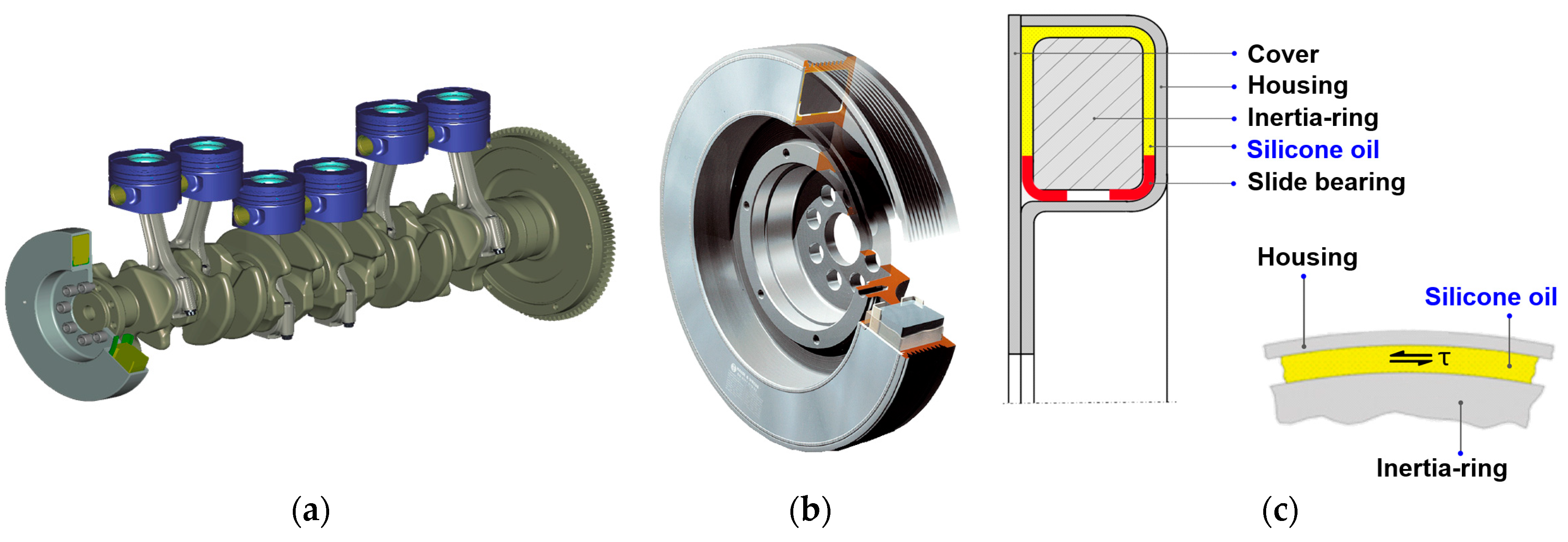
The vehicle industry primarily uses the torsional vibration dampers for the controlled damping of vibrations and oscillations. It is located at the free end of the crankshaft of reciprocating engines (see Figure 2a). Silicone oils have relatively high thermal stability, favorable tensile strength and density and have low friction properties thus they can effectively eliminate the torsional oscillations of the crankshaft in almost every frequency range. As the final stage of production process of viscous dampers, the structure of the damper is filled with silicone oil by using a special filling device. Because of the highly viscous nature of the oil and the narrow dimensions of the filling chamber (enclosed by the housing, cover, inertia-ring and bearings) (see Figure 2b,c), filling can take long time. The production time can be reduced by shortening the time required for the silicone oil entering in the system [3].

In order to properly use high viscosity silicone oils in basic research and industrial applications and to reduce the filling time of viscous torsional vibration dampers, it is essential to get to know the detailed rheological properties of PDMS, both in the linear and nonlinear viscoelastic range. In light of the rheological measurement results, a viscous (describing viscosity change) and elastic (multi-element Maxwell) model of the fluid can be developed. The obtained models are a fundamental input for advanced engineering software and for numerical simulations which enable quick, accurate and cost-effective analysis, design, and development of the viscous torsional vibration dampers. It is worth mentioning that there are several ongoing researches in conjunction with technical modelling and simulations, not only in the aeronautical industry [5,6], in the field of turbomachinery [7] and naval architecture [8], but in the all segments of the engineering sciences. This is because a significant amount of cost capacity and time can be saved by using different calculation techniques.

Most publications on rheological studies of polydimethylsiloxane are written for oils with a dynamic viscosity of 10 to 50 Pas or less [9,10]. Very few studies deal with high-viscosity silicone oils [11,12]. This can be explained by the fact that these materials are difficult to measure with the measurement capabilities of typical rheometers.

Kőkuti et al., in their studies [13,14,15,16], performed comprehensive rheological measurements on AK 1 000 000 STAB type silicone oil samples manufactured by Wacker Chemie, to investigate the temperature dependence of the viscoelastic behavior of the fluid in both linear and nonlinear ranges. Based on the measurement results, focusing on the elastic properties, they developed the constitutional equation of the oil with concentrated parameters. This equation consists of a constant-weighted, five-element White-Metzner model and was used to reproduce the Weissenberg effect during the rotational rheological measurement in the Comsol environment.

Syrakos et al. [17] linked the operating characteristics of a viscous dampener and the rheological behavior of the silicone oil used in the damper by applying three different rheological fluid models (Newton, Carreau–Yasuda, and Phan-Tien and Tanner) in numerical simulations. According to the results, the Newtonian model approximated creep and quasi steady-state flow well but did not take into account the hysteresis properties of the oil. The Carreau–Yasuda model described properly the viscous nature of the oil but did not model the elastic behavior. The Phan-Tien and Tanner model handled the viscous behavior of the oil similarly to the Carreau–Yasuda model and was also suitable for describing the elastic nature of the fluid with an appropriate hysteresis estimate.

Frings et al. [18] developed a mathematical model for a viscous vibration damper performing cyclic motion. The results of the model were compared with the experimental data. The damper model was also suitable for describing the fluid dynamic and thermal behavior of the silicone oil. The Carreau–Yasuda model was used as viscosity model for the oil, where the temperature dependence was also taken into account with a shifting factor. The numerical results showed that the model, despite its accuracy, tends to overestimate the decrease in damping force due to the change in viscosity caused by temperature increase. The authors also pointed out that, from a certain frequency value, the observed viscous hysteresis force–velocity relationship cannot be taken into account in a mathematical model that neglects the compressibility of the silicone fluid.

Abood et al. [19], in their study, made a comparison between experimental and numerical air–oil flow patterns in vertical pipe. A two-phase fluid dynamic simulation has been performed by utilizing volume of fluid (VOF) method to capture the phase boundary of air bubbles in the pipe filled with oil. During analysis the density, viscosity and temperature of the oil are set constant, and the surface tension between air and oil has to be taken into account. The effect of superficial velocity, gravity and length of pipe on movement and structure of air bubbles is discussed in detail.

Debnath et al. [20] investigated the flow of a non-Newtonian pseudoplastic fluid in pipes with different angles and shapes, in numerical a way, and compared the results with water flow. The analyzed fluid was considered isotherm, incompressible and time-independent, and the power law model was used to describe the fluid’s non-Newtonian behavior. The effect of the centrifugal and secondary flows caused by the pipe bend was explained, in detail, with the help of static and dynamic pressure, pressure drop, velocity field, viscosity, shear stress and shear-rate plots among others. The outcome of the numerical simulations was validated by experimental results.

Today, the viscous torsional vibration dampers have become more and more important in reciprocating engines, as the crankshaft has reduced stiffness due to the downsizing technology of the reciprocating engines for having higher performance, higher efficiency and lower emission.

The present case study, which is in conjunction with reciprocating engines via torsional vibration dampers, has strong business-related and economical background. The reciprocating engines market was valued at US$ 197,803.5 Million in 2017 and expected to reach US$ 271,508.6 Million in 2026, growing at a compounded annual growth rate (CAGR) of 6.5% from 2018 to 2026 [21].

The facts mentioned above motivated the authors to develop temperature- and shear-rate-dependent non-Newtonian viscosity model for a high viscosity silicone oil used in viscous torsional vibration dampers. The selected silicone oil must be a good representative of silicone fluids with a dynamic viscosity value between 200 and 2000 Pas (at 25 °C). Following the estimation of the model parameters with data used in Reference [13], and implementing the model in ANSYS FLUENT commercial software (2019 R1, ANSYS, Canonsburg, PA, USA, 2019), two transient silicone oil flow simulations were completed on elementary 3D tube geometry, in the size range of real viscous torsional vibration damper’s channels and filling chambers. The finite volume-based numerical results can provide information about flow characteristics of the silicone oil, including shear rate, viscosity and timeframe of the flow processes developed in different geometrical configurations.

2. The Applied Material, Instrument, Measurement Method and Adopted Results

Viscous torsional vibration dampers for heavy duty vehicles, trucks and ships require a high-viscosity silicone oil as working fluid, to meet the operational requirements for proper torsional vibration damping in almost any frequency ranges. According to Wacker Chemie’s website [22], AK 1 000 000 STAB silicone oil is suggested to be used in these devices; thus, the aim of the present paper is to develop a reliable, accurate, temperature- and shear-rate-dependent viscosity model of AK 1 000 000 STAB silicone oil for viscous torsional vibration damper applications. The authors found no available temperature- and shear-rate-dependent viscosity measurement data for AK 1 000 000 STAB silicone oil and for similar high-viscosity silicone oils on the website of Wacker Chemie or in scientific papers. Since Kőkuti et al. performed an extensive material research and model development for AK 1 000 000 STAB silicone oil with a large number of measurements in the preferred temperature and shear-rate ranges from viscous torsional vibration dampers’ manufacturing and operation point of view, the authors of this manuscript considered the viscosity, storage and loss moduli results with the applied rheological methods in Kőkuti et al.’s work [13,14] to be reliable, accurate and well-studied. Because of these facts, Kőkuti’s PhD dissertation [13,14] was used to adopt the measured rheological results and to deduce the necessary viscosity data from the storage and loss moduli curves presented in his work.

As reported in Kőkuti et al.’s works [13,14], Small Amplitude Oscillatory Shear (SAOS) tests have been performed on AK 1 000 000 STAB silicone oil sample, to determine the viscous properties of material. The Anton Paar Physica MCR 101 rheometer [23] was used for this purpose with CC10 (concentric cylinder with 10 mm inner gap) measuring head. This is a modern instrument that already includes air bearing (to reduce the friction loss) and strain-controlled measuring head (the shear stress in the sample is calculated from the instantaneous value of the current of the electric motor that rotates the measuring head in the sample). Above a given shear rate value, the Weissenberg effect can severely restrict the effectiveness and accuracy of the measurement, as the rotation causes a force in the oil sample parallel to the axis of rotation, which makes the sample to climb up on the measuring head and the instrument does not provide additional reliable measurement results [24]. To overcome this difficulty, the concentric cylinders measuring geometry should be replaced with cone-plate ones. The following data were recorded during the measurements:

-

Angular frequency (rad/s),

-

Storage and loss moduli (Pa),

-

Damping factor (-),

-

Deflection angle (mrad),

-

Torque (μNm).

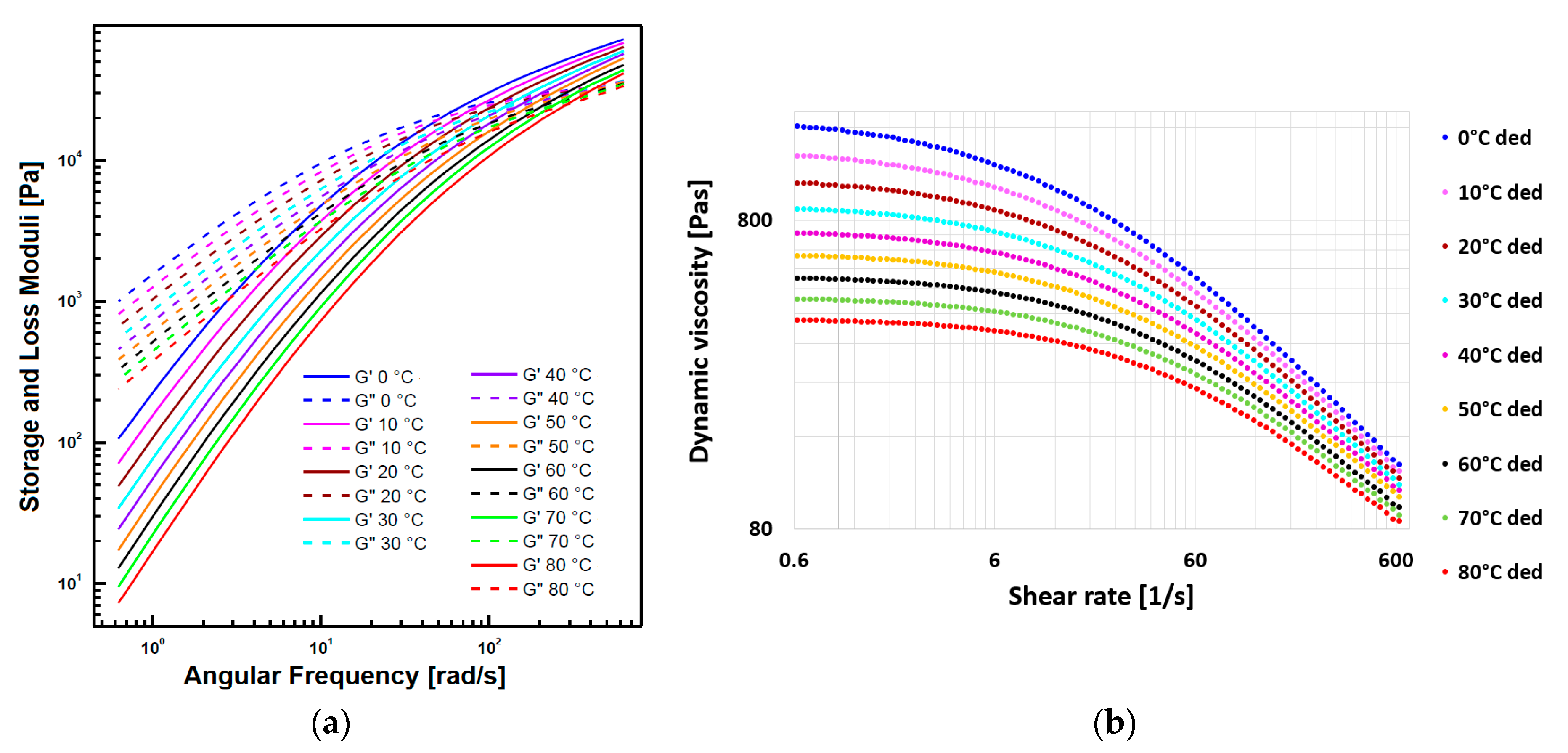
SAOS tests were performed on the silicone oil sample, at atmospheric pressure (1 bar), at different temperatures (0–80 °C by 10 °C temperature increment) and in the angular frequency range of 0.628–628 rad/s in 10 points per decade with 5% strain amplitude. The resting time before each measurement was selected to 15 min for reaching thermal equilibrium. Figure 3a shows the measured storage (solid lines) and loss (dashed lines) moduli for each temperature in the function of angular frequency with logarithmic axes. It turned out, from the SAOS tests, that the investigated oil behaves similarly in each temperature (curves can be vertically shifted into each other). Thus, AK 1 000 000 STAB obeys the so-called Time Temperature Superposition (TTS) principle.

The $\left|{\eta }^{*}\left(\omega \right)\right|$ absolute value of complex viscosity in the function of angular frequency can be calculated by Equation (1) [25], with the help of the $G\prime \left(\omega \right)$ storage and $G″\left(\omega \right)$ loss moduli in function of angular frequency. The dynamic viscosity, $\eta \left(\dot{\gamma }\right)$, in function of shear rate can be deduced from the absolute value of complex dynamic viscosity data based on the Cox–Merz rule expressed by Equation (2) [16]. The above-mentioned deduction process was done on 96 selected angular frequency values in the range of 0.628–628 rad/s, the temperature of each was taken from Figure 3a. Figure 3b shows the deduced dynamic viscosity data in function of shear rate with logarithmic axes. The viscous behavior of the oil depends not only on the temperature but also on the pressure, so it would be worthwhile in the future to perform similar rheological measurements at different pressures (above and below ambient pressure). As a first step of the present work, the goal is to mathematically describe the temperature dependence of viscosity data shown in Figure 3b, by estimating the parameters of a properly selected non-Newtonian viscosity model.

$$\left|{\eta }^{*}\left(\omega \right)\right|=\sqrt{{\left(\frac{G\prime \left(\omega \right)}{\omega }\right)}^2+{\left(\frac{G″\left(\omega \right)}{\omega }\right)}^2,}$$

(1)

$$\left|{\eta }^{*}\left(\omega \right)\right|={\eta \left(\dot{\gamma }\right)|}_{\omega =\dot{\gamma }}.$$

(2)

The geometric standard deviation was calculated for each storage and loss moduli curve obtained from rheological measurement at each investigated temperature (see

Table 1. Geometric standard deviation (GSD) values of storage and loss moduli curves.

Temperature	GSD of G′	GSD of G″
0 °C	6.728	2.903
10 °C	7.459	3.110
20 °C	8.222	3.316
30 °C	9.014	3.514
40 °C	9.821	3.707
50 °C	10.673	3.892
60 °C	11.403	4.068
70 °C	12.263	4.245
80 °C	13.048	4.408

).

3. Parameter Estimation

3.1. Carreau–Yasuda Viscosity Model

The Carreau–Yasuda model, which had been used in several previous works [17,18], is considered the most suitable for describing the viscous behavior of pseudoplastic non-Newtonian fluids in both the linear and nonlinear ranges. The general formula of the Carreau–Yasuda model is presented by Equation (3) [26]:

$$\eta \left(\dot{\gamma },T\right)={\eta }_{\infty }\left(T\right)+\left({\eta }_0\left(T\right)-{\eta }_{\infty }(T\right))\times {\left(1+{\left(\dot{\gamma }\times \lambda \left(T\right)\right)}^{a\left(T\right)}\right)}^{\frac{n\left(T\right)-1}{a\left(T\right)}}.$$

(3)

where$\dot{\gamma }—$current shear rate (1/s)$, T—$current temperature (°C)$, \eta \left(\dot{\gamma },T\right)—$shear-rate- and temperature-dependent current dynamic viscosity (Pas),${\eta }_{\infty }\left(T\right)—$temperature-dependent infinite-shear dynamic viscosity (Pas), ${\eta }_0\left(T\right)—$temperature-dependent zero-shear dynamic viscosity (Pas), $\lambda \left(T\right)—$temperature-dependent relaxation time (s),$a\left(T\right)—$temperature-dependent transition control factor (-) and$n\left(T\right)—$temperature-dependent power law index (-).

The material model of the silicone oil can be implemented in ANSYS FLUENT commercial software (2019 R1, ANSYS, Canonsburg, PA, USA, 2019), and the actual viscosity of the flow can be determined if the five temperature-dependent model parameters are known (each of them is non-negative in physical sense). The goal is, therefore, to determine the unknown model parameters in Equation (3) as a function of temperature.

3.2. Estimation of the Model Parameters

The relation indicated by Equation (3) is considered as the fitting function, and the introduced viscosity data in Figure 3 are used for parameter estimation. A variety of statistical optimization techniques are available in regression analysis for parameter estimation purpose, such as the least squares method, the least absolute deviation method, the M-estimation (maximum likelihood method) and S-estimation (scale method) or the least trimmed squares method. Even though the minimum sum method is also very competitive with the ordinary least squares method. In this work, the least squares method is used, considering its simplicity, effectiveness and completeness against any other methods. Additionally, the least squares method is widely used; it is a maximum-likelihood solution, and it is the best linear unbiased estimator [27,28].

The least squares functional contains the five model parameters with the deduced viscosity value (${\eta }_{N,T}$) at temperature, $T$, and with the selected shear-rate data, $\left({\dot{\gamma }}_N\right)$, according to Equation (4).

$${\epsilon }_T\left({\eta }_{\infty }\left(T\right),{\eta }_0\left(T\right),\lambda \left(T\right), a\left(T\right),n\left(T\right)\right)={\displaystyle \sum }_{N=1}^{96}{\left\{{\eta }_{N,T} -\left[{\eta }_{\infty }\left(T\right)+\left({\eta }_0\left(T\right)-{\eta }_{\infty }\left(T\right)\right)\times {\left(1+{\left({\dot{\gamma }}_N\times \lambda \left(T\right)\right)}^{a\left(T\right)}\right)}^{\frac{n\left(T\right)-1}{a\left(T\right)}}\right]\right\}}^2.$$

(4)

where${\epsilon }_T—$least squares functional containing the five model parameters at temperature, $T$;${\eta }_{\infty }\left(T\right),{\eta }_0\left(T\right),\lambda \left(T\right), a\left(T\right),n\left(T\right)—$unknown model parameters at temperature, $T$;$N—$sequence number of the current shear rate data;${\dot{\gamma }}_N—$Nth shear-rate data (1/s); and ${\eta }_{N,T}—$dynamic viscosity belonging to the N^th shear rate data at temperature $T$ (Pas).

The functional minimum is then gained by making the partial derivatives of the functional equal to zero according to Equations (5)–(9).

$$\begin{array}{l}\frac{\partial }{\partial {\eta }_{\infty }\left(T\right)}{\epsilon }_T\left({\eta }_{\infty }\left(T\right),{\eta }_0\left(T\right),\lambda \left(T\right), a\left(T\right),n\left(T\right)\right)={\displaystyle \sum }_{N=1}^{96}2\times \left\{{\left(1+{\left({\dot{\gamma }}_N\times \lambda \left(T\right)\right)}^{a\left(T\right)}\right)}^{\frac{n\left(T\right)-1}{a\left(T\right)}}-1\right\}\times \\ \left\{-\left({\eta }_0\left(T\right)-{\eta }_{\infty }\left(T\right)\right){\left(1+{\left({\dot{\gamma }}_N\times \lambda \left(T\right)\right)}^{a\left(T\right)}\right)}^{\frac{n\left(T\right)-1}{a\left(T\right)}}-{\eta }_{\infty }\left(T\right)+{\eta }_{N,T}\right\}=0,\end{array}$$

(5)

$$\begin{array}{l}\frac{\partial }{\partial {\eta }_0\left(T\right)}{\epsilon }_T\left({\eta }_{\infty }\left(T\right),{\eta }_0\left(T\right),\lambda \left(T\right), a\left(T\right),n\left(T\right)\right)={\displaystyle \sum }_{N=1}^{96}-2\times {\left(1+{\left({\dot{\gamma }}_N\times \lambda \left(T\right)\right)}^{a\left(T\right)}\right)}^{\frac{n\left(T\right)-1}{a\left(T\right)}}\times \{-\left({\eta }_0\left(T\right)-{\eta }_{\infty }\left(T\right)\right)\times \\ {\left(1+{\left({\dot{\gamma }}_N\times \lambda \left(T\right)\right)}^{a\left(T\right)}\right)}^{\frac{n\left(T\right)-1}{a\left(T\right)}}-{\eta }_{\infty }\left(T\right)+{\eta }_{N,T}\}=0,\end{array}$$

(6)

$$\begin{array}{l}\frac{\partial }{\partial \lambda \left(T\right)}{\epsilon }_T\left({\eta }_{\infty }\left(T\right),{\eta }_0\left(T\right),\lambda \left(T\right), a\left(T\right),n\left(T\right)\right)={\displaystyle \sum }_{N=1}^{96}-2\times \left(n\left(T\right)-1\right)\times {\dot{\gamma }}_N\times \left({\eta }_0\left(T\right)-{\eta }_{\infty }\left(T\right)\right)\times {\left({\dot{\gamma }}_N\times \lambda \left(T\right)\right)}^{a\left(T\right)-1}\times {\left(1+{\left({\dot{\gamma }}_N\times \lambda \left(T\right)\right)}^{a\left(T\right)}\right)}^{\frac{n\left(T\right)-1}{a\left(T\right)-1}}\\ \times \left\{-\left({\eta }_0\left(T\right)-{\eta }_{\infty }\left(T\right)\right)\times {\left(1+{\left({\dot{\gamma }}_N\times \lambda \left(T\right)\right)}^{a\left(T\right)}\right)}^{\frac{n\left(T\right)-1}{a\left(T\right)}}-{\eta }_{\infty }\left(T\right)+{\eta }_{N,T}\right\}=0,\end{array}$$

(7)

$$\begin{array}{l}\frac{\partial }{\partial a\left(T\right)}{\epsilon }_T\left({\eta }_{\infty }\left(T\right),{\eta }_0\left(T\right),\lambda \left(T\right), a\left(T\right),n\left(T\right)\right)={\displaystyle \sum }_{N=1}^{96}\{\frac{\left(n\left(T\right)-1\right)\times {\left({\dot{\gamma }}_N\times \lambda \left(T\right)\right)}^{a\left(T\right)}\times \ln \left({\dot{\gamma }}_N\times \lambda \left(T\right)\right)}{a\left(T\right)\times \left(1+{\left({\dot{\gamma }}_N\times \lambda \left(T\right)\right)}^{a\left(T\right)}\right)}-\frac{\left(n\left(T\right)-1\right)\times \ln \left(1+{\left({\dot{\gamma }}_N\times \lambda \left(T\right)\right)}^{a\left(T\right)}\right)}{a{\left(T\right)}^2}\}\times \\ \{-\left({\eta }_0\left(T\right)-{\eta }_{\infty }\left(T\right)\right)\times {\left(1+{\left({\dot{\gamma }}_N\times \lambda \left(T\right)\right)}^{a\left(T\right)}\right)}^{\frac{n\left(T\right)-1}{a\left(T\right)}}-{\eta }_{\infty }\left(T\right)+{\eta }_{N,T}\}=0,\end{array}$$

(8)

$$\begin{array}{l}\frac{\partial }{\partial n\left(T\right)}{\epsilon }_T\left({\eta }_{\infty }\left(T\right),{\eta }_0\left(T\right),\lambda \left(T\right), a\left(T\right),n\left(T\right)\right)={\displaystyle \sum }_{N=1}^{96}\frac{-2}{a\left(T\right)}\times \left({\eta }_0\left(T\right)-{\eta }_{\infty }\left(T\right)\right)\times {\left(1+{\left({\dot{\gamma }}_N\times \lambda \left(T\right)\right)}^{a\left(T\right)}\right)}^{\frac{n\left(T\right)-1}{a\left(T\right)}}\\ \times \ln \left(1+{\left({\dot{\gamma }}_N\times \lambda \left(T\right)\right)}^{a\left(T\right)}\right)\times \left\{-\left({\eta }_0\left(T\right)-{\eta }_{\infty }\left(T\right)\right)\times {\left(1+{\left({\dot{\gamma }}_N\times \lambda \left(T\right)\right)}^{a\left(T\right)}\right)}^{\frac{n\left(T\right)-1}{a\left(T\right)}}-{\eta }_{\infty }\left(T\right)+{\eta }_{N,T}\right\}=0.\end{array}$$

(9)

Parameter estimation with the Carreau–Yasuda fitting function requires nonlinear regression. Considering the complexity of the above derivatives, the approximation of the system of five nonlinear equations of the least-squares functionals is solved iteratively. There are numerous root-finding algorithms for the approximation of the solution, such as Newton’s method, secant method, bisection method or gradient method (gradient descent or conjugate gradient). Due to the fact that Newton’s method uses second-order derivatives and the order of its convergence is quadratic, it provides precise approximation in less iteration steps, as compared to any other approximation techniques [29]. However, based on the private communication with F. Pápai, generating the elements of the 5 × 5 Jacobian matrix required for the calculation would be cumbersome and time-consuming. Instead, the quasi-Newtonian method was used, where the elements of the Jacobian matrix are replaced by approximation and the problem is traced back to extremum search. MathCad 15 was used for the calculation outlined. Considering Equation (4), for example, a least square functional with five model parameters was written for each selected temperature case (9 equations and 45 unknown parameters). The “Minimize” function, based on the nonlinear quasi-Newton principle, available in the mathematical software, was used to find the minimum of the functional. To enhance the convergence, the initial values of the unknown parameters before the first iteration were set as follows. The initial values for $\lambda \left(T\right)$, $a\left(T\right)$ and $n\left(T\right)$ were selected according to Reference [26], while the initial value of ${\eta }_{\infty }$ was chosen for 0 Pas at all temperatures, and the initial value of ${\eta }_0$ was determined based on the deduced viscosity at the given temperature and at the lowest recorded shear rate (0.628 1/s). An additional setting was required to specify the constraints: The unknown model parameters could only take non-negative values. At the end of the iteration, the estimated parameters for each investigated temperature were gained, which satisfied the sign constraint and provided the least squares deviation in the examined shear-rate range.

3.3. Temperature Dependence of the Estimated Model Parameters

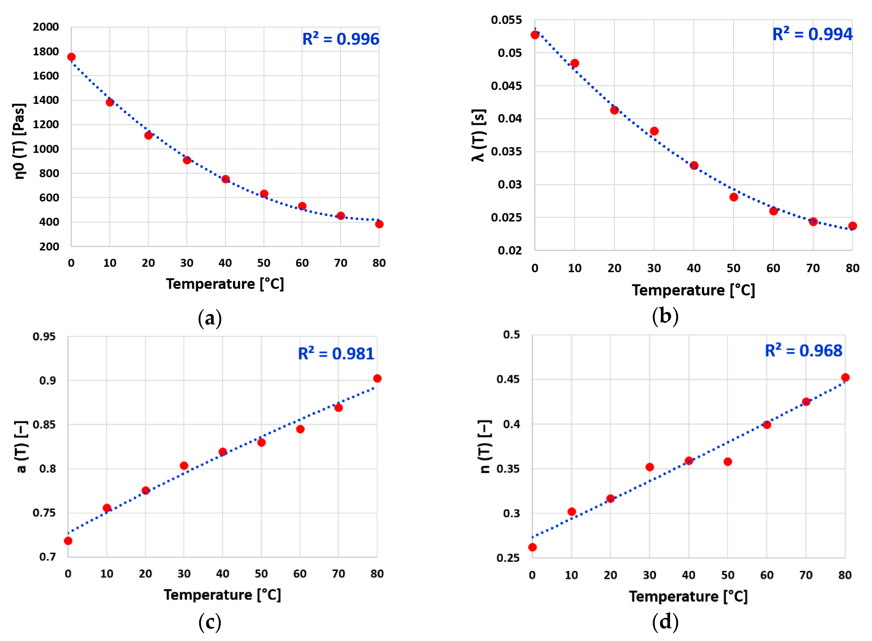
The red dots in Figure 4 show the estimated model parameters at the investigated temperatures. While the infinite-shear dynamic viscosity parameter value was set to zero based on the literature [17,30,31,32,33,34,35], the relaxation-time parameter values show a monotonically decreasing trend with increasing temperature. The transition control factor parameter values and the power law index parameter values show a monotonically increasing trend with increasing temperature. The temperature dependence of the plotted parameter values was approximated by a quadratic function according to Equation (10):

$$P\left(T\right)=p_1\times T^2+p_2\times T+p_3.$$

(10)

where $T$ is the current temperature (°C); $P\left(T\right)$ is an estimated model parameter, ${\eta }_0\left(T\right), \lambda \left(T\right), a\left(T\right)$ or $n\left(T\right)$, on a given $T$, temperature; and $p_1$, $p_2$ and $p_3$ are parameters of the approximate quadratic curve (quadratic parameters) [-].

Using the $P\left(T\right)$ estimated model parameter values for each investigated temperature, $T$, the $p_1$, $p_2$ and $p_3$ quadratic parameters of the fitting function can be determined for each model parameter, using the pseudoinverse of the coefficient matrix according to matrix Equation (11). $\underset{\_}{\mathit{P}}$ denotes the column vector of the parameter values${\eta }_0\left(T\right), \lambda \left(T\right), a\left(T\right)$ or $n\left(T\right)$, and $\underset{\_}{\mathit{p}}$ denotes the column vector of the quadratic parameters of the quadratic curve fitted to the parameter values at temperature, $T$, in Equation (11). Matrix Equation (11) is solved according to Equation (12).

$$\underset{\_}{\underset{\_}{\mathit{Q}}}\times \underset{\_}{\mathit{p}}=\underset{\_}{\mathit{P},}$$

(11)

$$\underset{\_}{\mathit{p}}={\underset{\_}{\underset{\_}{\mathit{Q}}}}^{+}\times \underset{\_}{\mathit{P},}$$

(12)

where the pseudoinverse of the $\underset{\_}{\underset{\_}{\mathit{Q}}}$ coefficient matrix is given by Equation (13).

$${\underset{\_}{\underset{\_}{\mathit{Q}}}}^{+}={\left({\underset{\_}{\underset{\_}{\mathit{Q}}}}^T\times \underset{\_}{\underset{\_}{\mathit{Q}}} \right)}^{-1}\times {\underset{\_}{\underset{\_}{\mathit{Q}}}}^T.$$

(13)

The results of the parameter estimation performed on 96 selected data at each temperature investigated (total number of evaluated viscosity data is 864) are summarized by the equations of Carreau–Yasuda model parameter curves, according to Equations (14)–(18) in the investigated temperature (0–80 °C) and shear-rate (0.628–628 1/s) range for AK 1 000 000 STAB silicone oil.

$${\eta }_{\infty }\left(T\right)\cong 0,$$

(14)

$${\eta }_0\left(T\right)=0.199\times T^2-32.146\times T+1.714\times {10}^3,$$

(15)

$$\lambda \left(T\right)=3.552\times {10}^{-6}\times T^2-6.656\times {10}^{-4}\times T+5.367\times {10}^{-2},$$

(16)

$$a\left(T\right)=-3.601\times {10}^{-6}\times T^2+2.356\times {10}^{-3}\times T+0.727,$$

(17)

$$n\left(T\right)=1.403\times {10}^{-6}\times T^2+2.055\times {10}^{-3}\times T+0.273.$$

(18)

Figure 4 shows not only the estimated model parameters (red dots) but also the fitted model parameter curves as a function of temperature (dotted lines) and the R-squared values in the right upper corner of the diagrams. See the interpretation of the presented results at the end of this chapter.

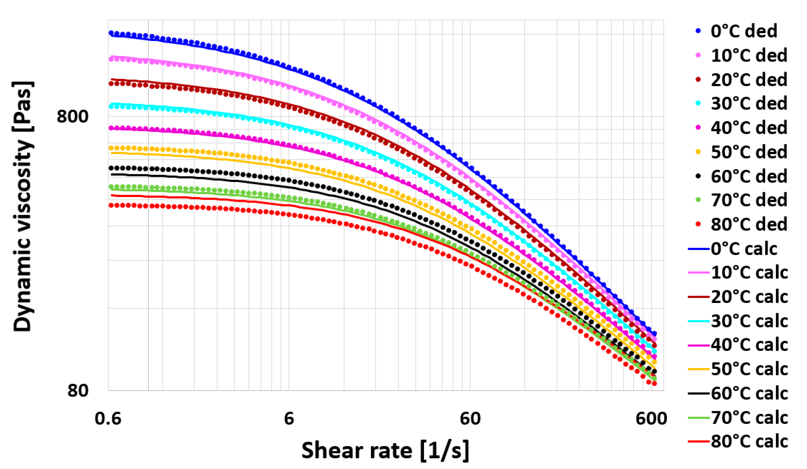
Figure 5 shows the deduced viscosity values (dots) and the viscosity curves (lines) calculated by Equations (3) and (14)–(18), as a function of shear rate at each investigated temperature.

The highest deviation between the deduced and the calculated viscosity data is found to be 34 Pas (relative deviation of 9%), at 80 °C, on 0.676 1/s shear rate; thus, the temperature-dependent viscosity model obtained by parameter estimation is suitable for use in non-Newtonian transient simulation calculated by ANSYS FLUENT commercial software (2019 R1, ANSYS, Canonsburg, PA, USA, 2019).

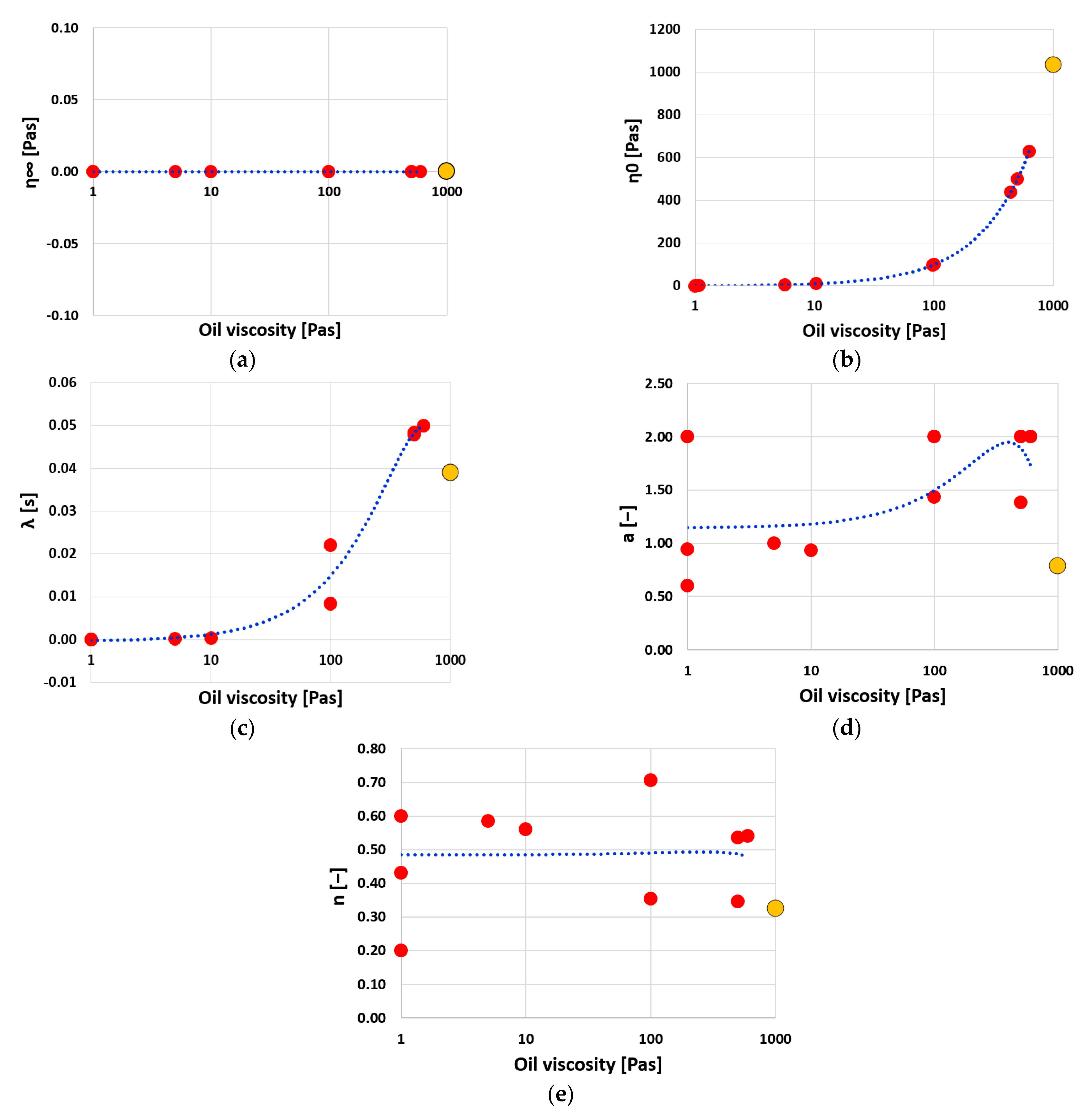
Based on available the literature data, the parameter estimation results of silicone oil with six different viscosities (1, 5, 10, 100, 500 and 600 Pas) were compared to the obtained model parameters of the current work, at room temperature, in Figure 6. The comparison shows a good coincidence, as the parameters fit the trend line or are situated in the close scatterplot of the literature data. See the interpretation of the presented results after Figure 6.

Zero-shear dynamic viscosity, ${\eta }_0\left(T\right)$, is actually the initial viscosity of the oil. As temperature raises, oil molecules have greater thermal energy and are more easily able to overcome the attractive forces binding them together across fluid layers, resulting in viscosity reduction and in a more fluent behavior (see Figure 4a). The increase in the number of repeating monomer units in the PDMS chain causes longer molecule chains, which are more likely to be entangled and result in higher viscosity (see Figure 6b).

Relaxation time, $\lambda \left(T\right)$, represents the time for the shear stress to decay by a factor after the oil stops being sheared. The temperature dependence of the relaxation time can be described by a $\tau$ correlation time that is often assumed to follow an Arrhenius law, according to Equation (19). Because of this fact, increasing temperature results in relaxation time decrease (see Figure 4b). Higher viscosities increase the activation energy that then result in higher relaxation time (see Figure 6c).

$$\tau \left(T\right)={\tau }_0\times e^{\frac{E}{k_B\times T}}.$$

(19)

where$\tau$—correlation time,$T—$temperature,${\tau }_0—$time constant,$E—$activation energy and$k_B—$Boltzmann constant.

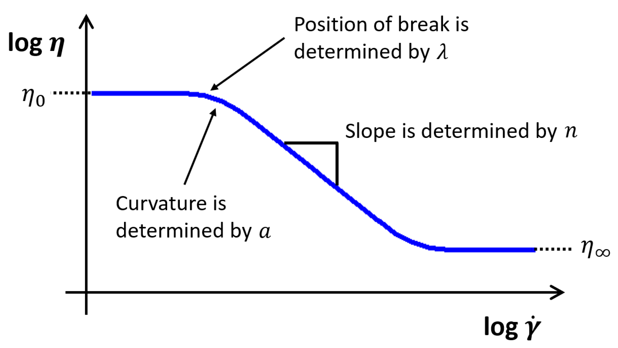
Transition control factor, $a\left(T\right)$, is a dimensionless parameter that describes the transition from the zero-shear rate region to the rapidly decreasing power law region of the viscosity versus shear rate curve. The higher this value at higher temperatures, the sharper the transition (see Figure 7).

Power law index $n\left(T\right)$ is another dimensionless parameter in the model that describes the slope of the rapidly decreasing region of viscosity versus shear rate curve (see Figure 7).

As stated in Morrison’s rheology book [36], Carreau–Yasuda model does not provide molecular insight into the polymer behavior. Consequently, only zero-shear dynamic viscosity ${\eta }_0\left(T\right)$ and relaxation time $\lambda \left(T\right)$ can be explained from physical point of view.

4. Numerical Transient Fluid Dynamic and Heat-Transfer Simulations

The aim of the simulations is to achieve the following:

i.

Apply and test the viscous behavior of AK 1 000 000 STAB silicone oil described by the viscosity curves of the Carreau–Yasuda model,

ii.

Gather fundamental design information about advantages/disadvantages on different variations of cross-sectional area of the flow field.

One of the most interesting question is—which we seek the answer to in this section—how the different channel shapes influences the speed of the flow front, the through-flow time in the channel in the function of temperature and why in case of the investigated non-Newtonian fluid. This information can provide new information and supports the design and developments of the torsional vibration dampers, not only in the nominal operation, but also in the production process.

4.1. Simulation Model

ANSYS FLUENT commercial software (2019 R1, ANSYS, Canonsburg, PA, USA, 2019) was used for flow modeling purposes; it is a computational fluid dynamics program suitable for handling multiphase flows, too. The exact solution of the governing equations (conservation law of mass, energy and momentum) is approximated—followed by the discretization of the flow field— in an iterative way based on the finite volume method. The governing equations are written in a compact and versatile form in Equation (20) [37].

$$\frac{\partial }{\partial t}{{\displaystyle \int }}_V^{}\rho \Phi dV+{{\displaystyle \oint }}_A^{}\rho \Phi V\times dA={{\displaystyle \oint }}_A^{}{\Gamma }_{\Phi }\nabla \Phi \times dA+{{\displaystyle \int }}_V^{}{S}_{\Phi }dV.$$

(20)

where$t—$time,$V—$domain volume,$\rho —$density,$A—$domain surface,$S—$source term,$\Gamma —$circulation,$\nabla —$nabla operator and $\Phi —$equation type parameter

If $\Phi$ = 1 → continuity equation,$\Phi$ = $u$ → momentum equation in X direction,$\Phi$ = $v$ → momentum equation in Y direction,$\Phi$ = $w$ → momentum equation in Z direction and$\Phi$ = $h$ → energy equation.

The interface between two different phases (silicone oil and air in this study) is calculated by Volume of Fluid (VOF) method. VOF is an advection scheme that allows us to track the shape and position of the interface in any timestep. The method is based on use of a fraction function that is defined as the integral of a fluid’s characteristic function in a mesh cell. The derivative of the fractional function must be equal to zero, as presented in Equation (21) [38].

$$\frac{\partial C}{\partial t}+v\times \nabla C+\nabla \times \left[C\left(1-C\right)U_r\right]=0.$$

(21)

where$t—$time,$C—$fractional function (phase interface is situated where 0 $\le C\le$ 1; $C$= 1 means the cell is full of fluid),$v—$fluid velocity,$U_r—$an artificial force that compresses the region under consideration and $\nabla —$nabla operator.

Three-dimensional elemental tube geometry, built up from three different tube sections in the size range of a real viscous torsional vibration damper’s channels and filling chamber, was used in the flow analysis.

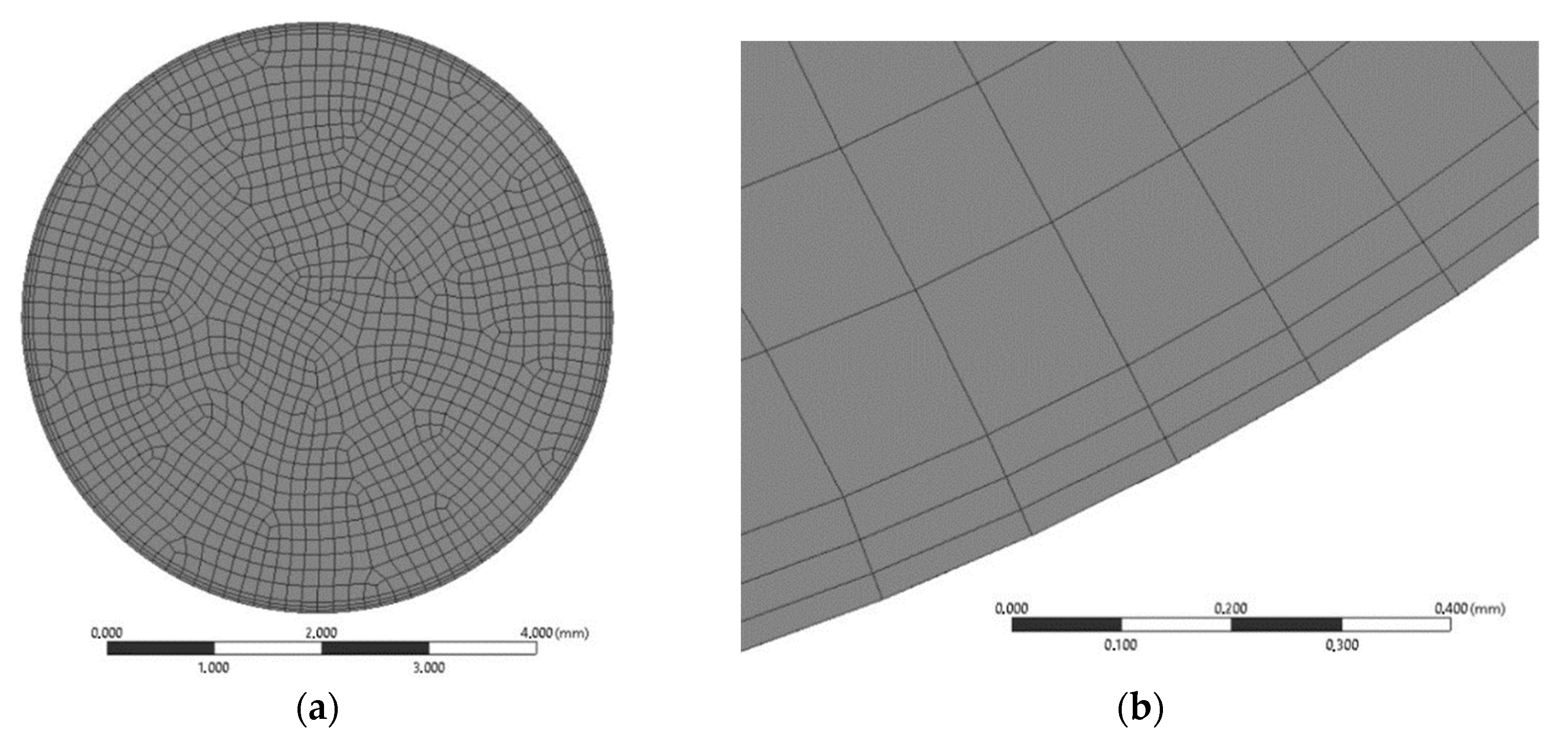
The length of the tube is 30 mm (see Figure 8a,b), with a maximum diameter of 5.5 mm and a minimum diameter of 2 mm, as shown in Figure 8a. The numerical mesh is built up from 0.15 mm hexagonal and prism elements with a total number of 299,088 elements (312,494 nodes), and the boundary layer close to the wall is also considered with a division of three sublayers, according to Figure 9b. The prism elements in these sublayers are generated in smooth transition option with 0.3 transition ratio and with 1.35 grow rate.

4.2. Boundary Conditions and Material Properties

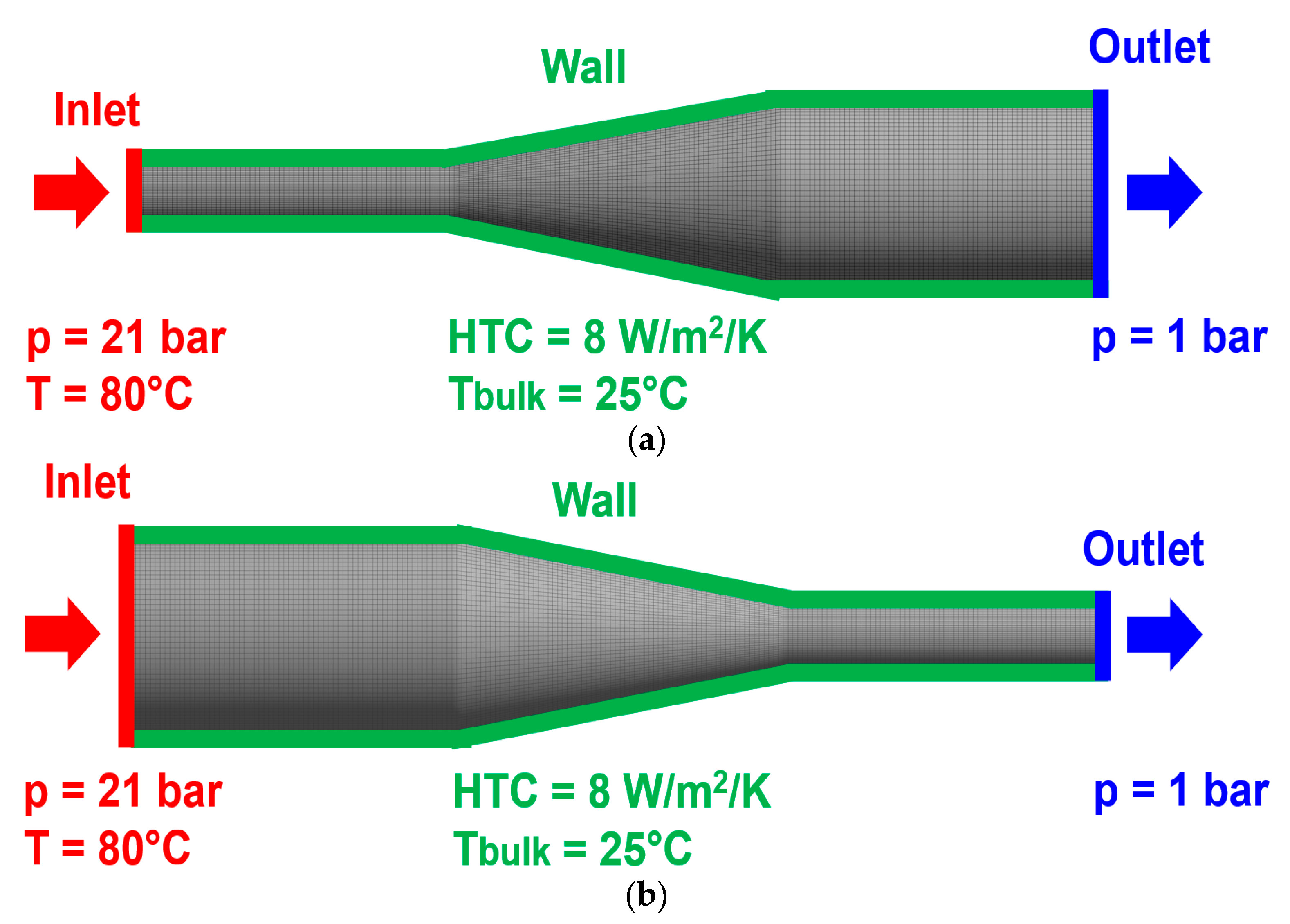
Two simulation cases were performed on the tube geometry presented in Section 4.1. In the first case, called diffuser simulation, the “Inlet” boundary condition was defined on the tube end with smaller diameter, while the other end of the tube, with the larger diameter, was set as “Outlet” boundary. In the second case, called confusor simulation, the roles of the boundaries are replaced according to Figure 10a,b. A total pressure of 21 bar on the “Inlet” boundary passes silicone oil at 80 °C, through the tube against the “Outlet” boundary that is at atmospheric pressure (1 bar).

The tube walls were defined as non-slip and smooth (zero surface roughness) with a heat-transfer coefficient (HTC) of 8 W/m²/K [39], where the temperature far away from the tube (Tbulk) was 25 °C.

Due to the high viscosity of the silicone fluid, laminar flow was assumed (based on preliminary calculations where the Reynolds number was found to be less than 1) over the entire flow domain for both simulation cases. The density of silicone fluid was described by Equation (22) [40] where $\rho \left(25 °\mathrm{C}\right)=970 \mathrm{kg}/{\mathrm{m}}^3$ and its viscosity was described by the Carreau–Yasuda model formulated by Equation (3), in which the temperature-dependent model parameters were defined by Equations (14)–(18).

$$\rho \left(T\right)=\frac{\rho \left(25 °\mathrm{C}\right)}{1+9.2\times {10}^{-4}\times \left(T-25\right)+4.5\times {10}^{-7}{\left(T-25\right)}^2} .$$

(22)

The considered silicone oil has an initial (zero-shear) dynamic viscosity around 1000 Pas at 25 °C, which would have made it not sufficiently fluent and would have led to a longer processing time. Therefore, similarly to the realistic operational conditions, the simulation was performed with a heated oil at 80 °C, at which the initial (zero-shear) dynamic viscosity is only 380 Pas. The density (1.225 kg/m³) and viscosity (1.7894 × 10⁻⁵ Pas) of the air were considered to be temperature-independent. A temperature-independent surface tension (0.02 N/m) was set at the interface of silicone oil and air, according to Reference [41]. In the first iteration step of the transient simulation, there was no oil in the tube, and in the next iteration steps, the current position of the oil front propagating during subsequent iterations was determined by the volume fraction function. The numerical results of the investigated tube flows are discussed in Section 4.3.

4.3. Numerical Simulation Results

A mesh-sensitivity analysis was performed on confusor simulation case with seven different mesh refinements in order to verify the mesh independency in the numerical results. Four different flow parameters (velocity, dynamic viscosity, shear rate and fluid volume fraction) were investigated in the same node and in the same flow time. It turned out, from the analysis, that the averaged relative difference (related to the reference mesh with element number of 299,088) in the parameters is 5.46% with a coarser mesh, while this value is 3.64% with a finer mesh. Thus, the numerical results are considered mesh-independent from element number 299,088 and above.

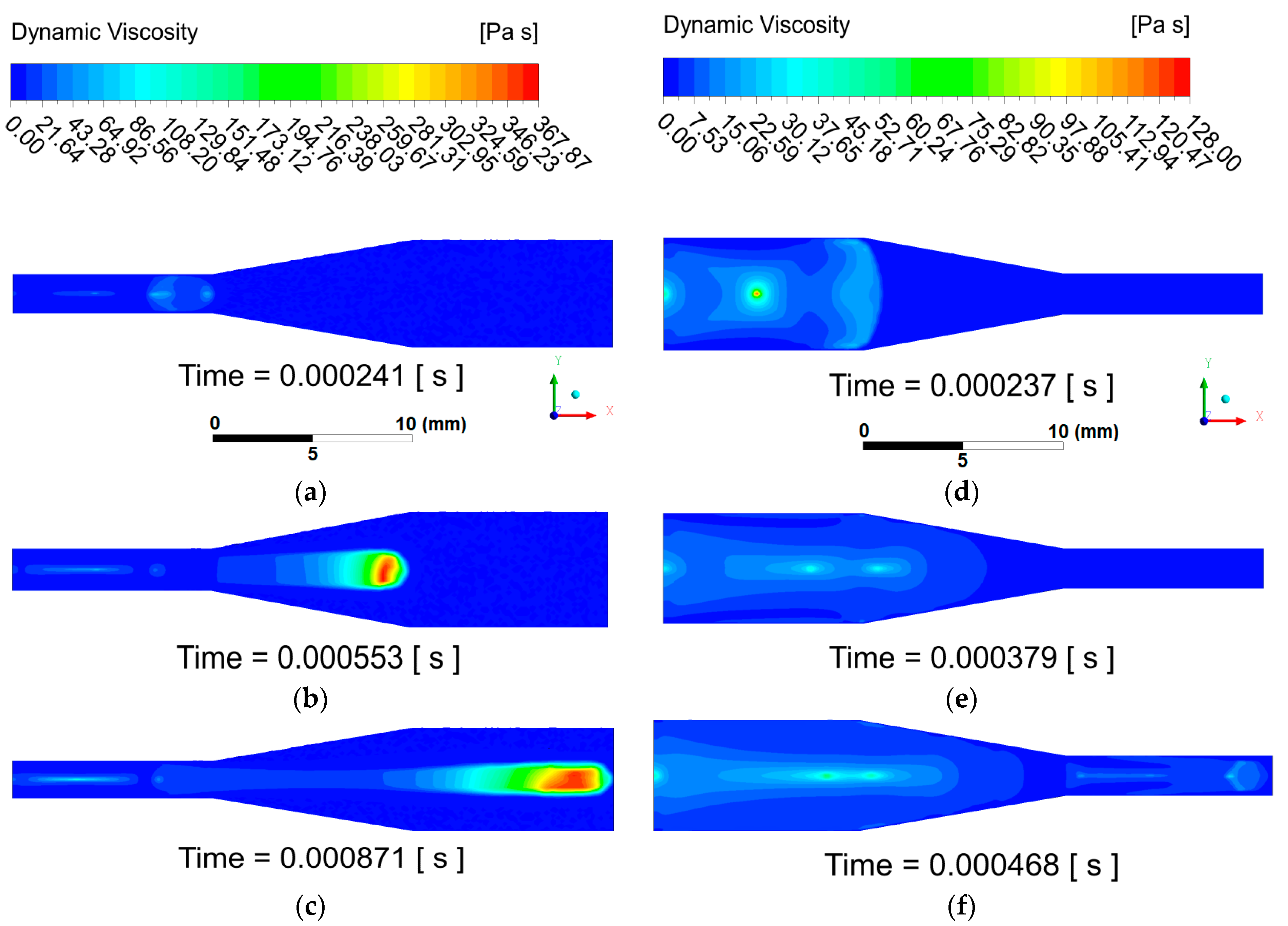
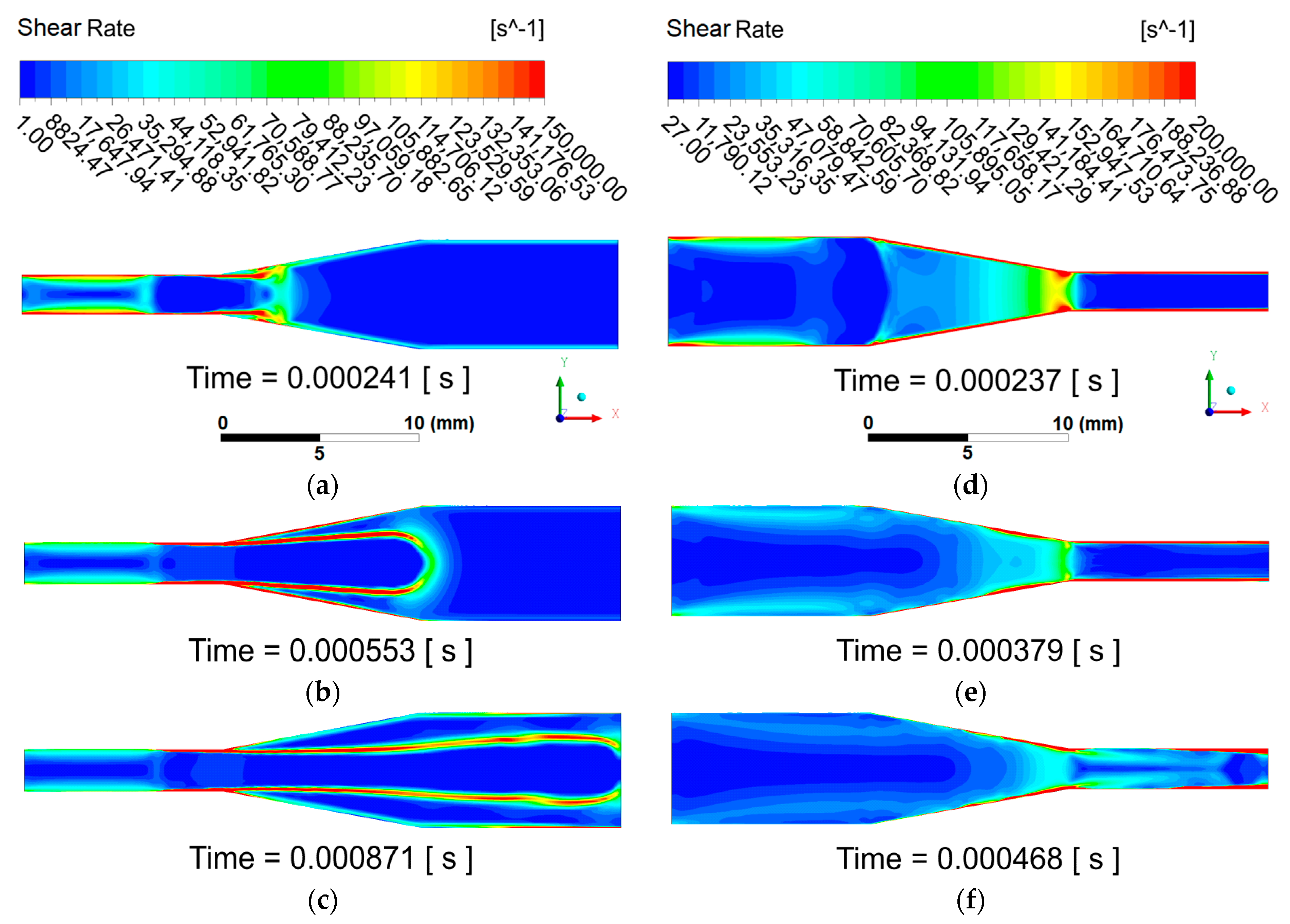
The distribution of dynamic viscosity (see in Figure 11) and the shear rate (see in Figure 12) obtained from the numerical results is plotted in the symmetry plane of the tube geometry. Three timesteps from the whole transient analysis were selected to present the results and discuss the fluid dynamic phenomena related the non-Newtonian behavior. The first timestep is the moment when the silicone fluid takes one-third of the length of the tube. The second timestep corresponds to the moment when two-thirds of the length of the tube are taken by the oil and the “Outlet” is reached in the third timestep. The same legend was used in each timestep per variable per simulation case.

The transient simulation results reveal the fact that, in the diffuser simulation case, the oil front decelerates continuously along the entire length of the tube, while in confusor simulation case, by entering the second tube section, there is an increase in the oil front velocity. The filling time of the tube in Figure 11f is less by 0.000403 s, compared to Figure 11c, which means that the flow front moves faster in confusor case. The oil flow remains cohesive in both simulations until the “Outlet” boundary is reached. Although the shorter filling time is rather due to the higher mass flow rate (higher inlet cross-section), it is also affected by higher shear rate and lower viscosity.

Dynamic viscosity results demonstrate that, in the diffuser simulation case, a free jet of silicone fluid forms (see definition in next paragraph) in the tube, and the viscosity of the oil jet behind the oil front increases continuously. The oil in the first tube section is sufficiently fluent (see Figure 11a) due to the low viscosity values (viscosity maximum: 50 Pas). In the second and third tube sections (Figure 11b,c), the environment of the oil front becomes highly viscous (viscosity maximum: 367.87 Pas), approaching the initial viscosity value of 380 Pas (zero shear). The continuous deceleration of the oil jet can be partially explained by the gradual increase of viscosity in the free jet of silicone oil.

The term “formation of free jet of silicone oil” refers to the following phenomenon according to Figure 11b,c: Silicone oil maintains its fluent properties (low viscosity) while the sample is under continuous shearing (see along the tube walls). In case the oil front passes through the diffusor, the cross-section expands, and the flow front loses the contact with the wall. As a result, the oil stops being sheared, and the viscosity starts increasing. It forms a free jet along the longitudinal axes of the tube inside of the flow front (where the viscosity increases to maximum value belong to the given temperature).

In the confusor simulation case, the opposite phenomenon can be observed. The reason for the velocity increment at the “Outlet” is, besides the geometrical shape (higher mass flow rate due to higher inlet cross-section), the reduction of viscosity in the second tube section. When the end of the first tube section is reached (see Figure 11d), the viscosity of the oil reaches its maximum (128 Pas) in the center line of tube. As the flow front enters the third tube section (see Figure 11e), the viscosity maximum drops to about 35 Pas, and the oil becomes sufficiently fluent. At the moment of reaching the “Outlet” boundary (see Figure 11f), the viscosity maximum raises to 60 Pas in the center line of the tube.

The reason of the continuous flow deceleration and gradual viscosity increase in the free jet of silicone oil experienced in the diffuser simulation can be found in the evolution of the shear rate. Because the silicone oil is a shear-thinning non-Newtonian fluid, the viscosity remains low only in areas of the flow domain where the shear rate is sufficiently high. The oil is sheared highly only close to the wall of the first tube section as shown in Figure 12a–c (maximum shear rate: 150,000 1/s), but as the oil front moves towards it, the shear rate values adjacent to the wall continuously decrease. Additionally, viscosity values are continuously increasing in the center part of the first tube section, and they are decreasing in a radial direction. By the end of the simulation, the shear rate adjacent to the wall in the first tube section is decreased to 75,000 1/s because of deceleration, while the shear rate at the center line of the tube is around 1 1/s. Apart from the first tube section, in the rest of the flow domain, the oil suffers from a negligible shear (1 1/s), which results in the formation of free jet of silicone oil with low shear and a continuous increase in viscosity. The maximum shear rate values around the oil jet, developed in the second and third tube sections, are caused by the high velocity difference between the oil and air.

In case of confusor simulation, the longitudinal size of the higher shear rate zones adjacent to the wall in the first tube section increases continuously as the oil front moves forward (see Figure 12d,e). Reaching the narrowest cross-section of the tube geometry, the oil suffers from additional and constant shear along the wall of the constriction (shear rate maximum: 200,000 1/s), resulting viscosity drop. At the moment of reaching the “Outlet” (see Figure 12f), oil remains under high shear in the constriction and in the entire third tube section, which, besides the geometrical shape (high inlet cross-section and thus high mass flow rate), provide sufficiently fluent flow and shorter through-flow (faster filling) time, compared to the diffuser simulation case. The shear rate minimum is 27 1/s in the center line of the first tube section.

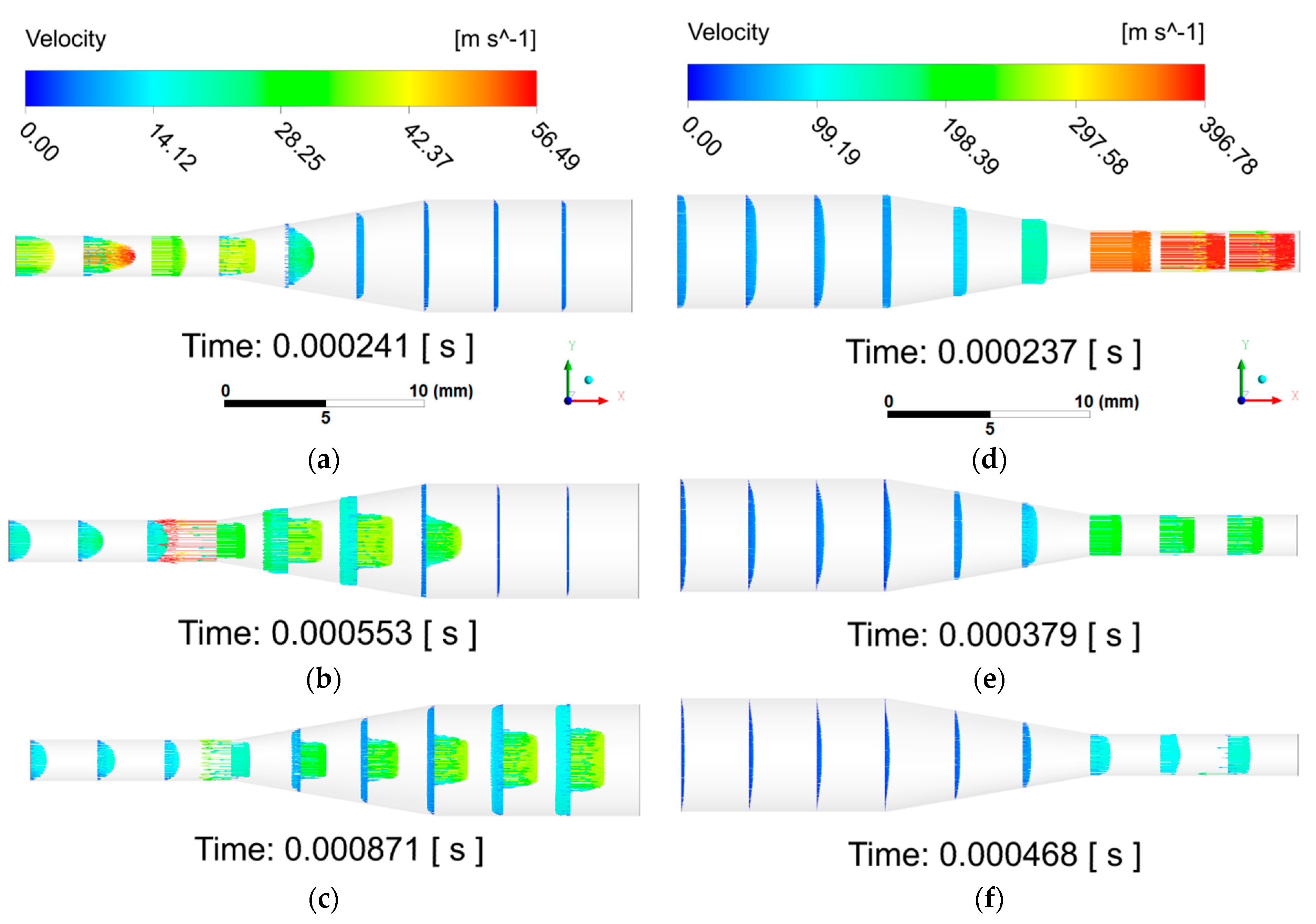
Figure 13 displays the velocity profile by vectors along the geometry for both diffuser and confusor simulation case in the selected timesteps. The free jet of silicone oil propagation through the calm air domain can be well observed in Figure 13a–c. In terms of confusor simulation case, high velocity vectors (see Figure 13d,e) show well how the air is pushed out of the straight tube with smaller diameter by the oil.

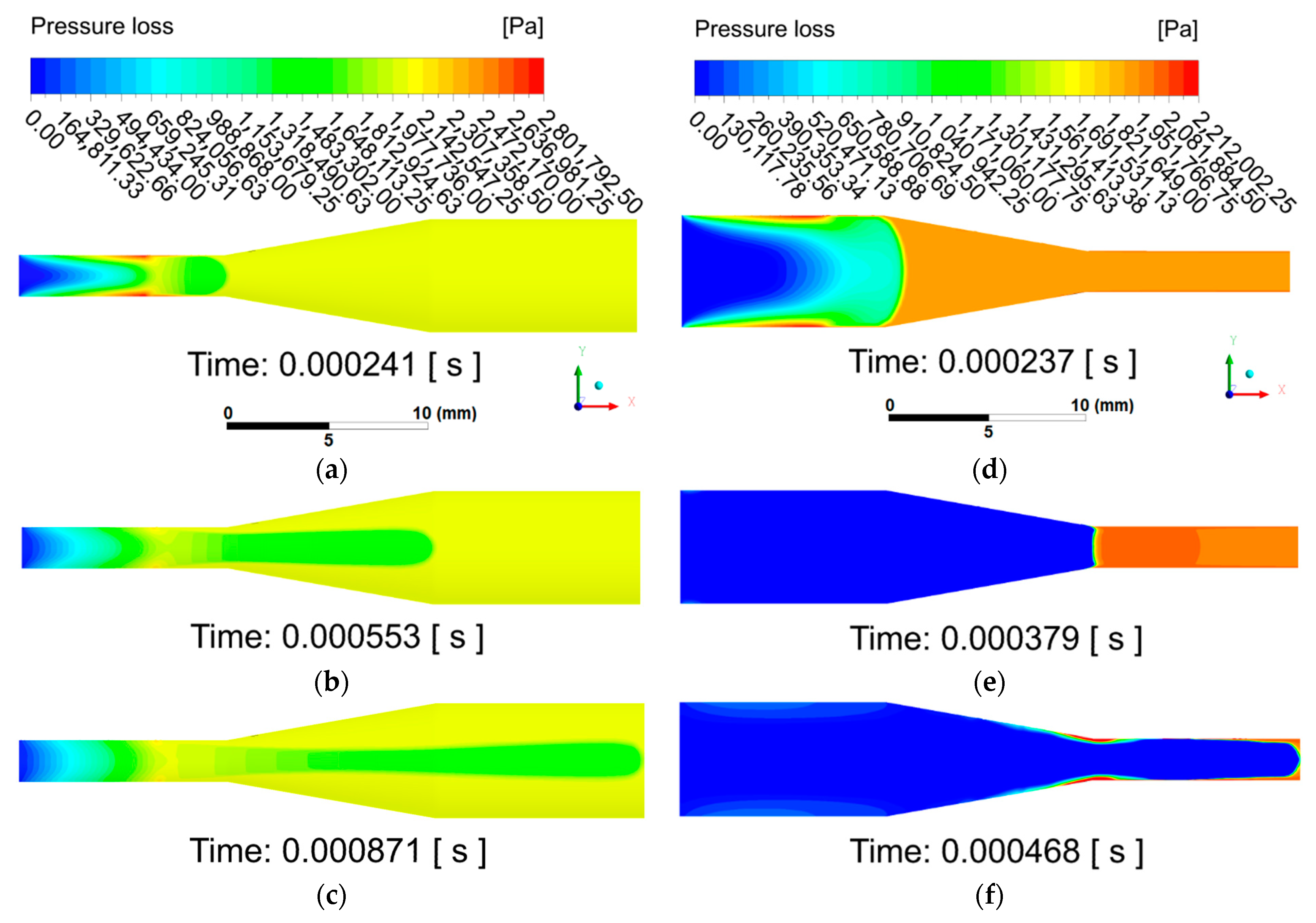
Figure 14 presents the pressure loss distribution along the geometry for both diffuser and confusor simulation case in the selected timesteps. Region of silicone oil and of air can be well distinguished from each other based on the pressure loss values along the flow domain.

It turned out, from the simulation results, that the formation of free jet of silicone fluid (low shear) slows down gradually; thus, it should be avoided for through-flow/filling time reduction. Since silicone oil has pseudoplastic (shear thinning) properties, the deceleration of the fluid (as shear rate decreases) causes the viscosity to increase. As a result of viscosity increase, the fluid suffers from further deceleration in the whole flow domain. In the filling process of viscous torsional vibration dampers, the goal is to minimize the viscosity by ensuring a permanent contact of the silicone oil with the housing, inertia-ring and cover (oil is under continuous shear near the walls) throughout the filling process, in order to avoid the formation of free jet flow. A further investigation is in progress, to determine effect of the dissipated heat for the process.

5. Conclusions

The application range of the silicone oils is increasing continuously; they are frequently used in energetics, vehicle engineering, astronautics and medical sciences. This material operates as lubricant and working fluids of transformers, diffusion pumps, fluid heaters and torsional vibration dampers in high power reciprocating engines. It requires accurate material models in the field of technical modeling and simulations, in order to reproduce different processes virtually with high precision (the average relative deviation between the measured and computed results should be less than or equal to 5%) in the entire lifetime cycle of the products.

Hence, a novel temperature- and shear-rate-dependent Carreau–Yasuda viscosity model equation was developed for the AK 1 000 000 STAB type silicone oil, verified and applied in a CFD code for testing and determining the effect of increasing and decreasing flow cross-sectional area with especial care for the speed of the flow-front and so the through-flow time.

Based on the available rheological measurement results of the high-viscosity silicone oil AK 1 000 000 STAB [13], which is a generally used material in damping technology, nonlinear regression and quadratic parameter estimation have been performed to develop a temperature-dependent (0–80 °C) and shear-rate-dependent (0.628–628 rad/s) Carreau–Yasuda viscosity model. Error analyses of the curve fitting for the model parameters and viscosity values were completed. The obtained model parameters show a good agreement with the parameters taken from the available literature. The developed viscosity model was applied in a validated finite-volume-method-based engineering software in multiphase transient simulations. The mesh and parameter sensitivity analyses were completed. Converged solutions were reached in each investigated case. Three-dimensional converging and diverging nozzle-geometries were considered in the analyses. The size ranges of the flow domains were determined in such a way that would fit with the dimensions of a real viscous torsional vibration damper’s channels and chambers, in order to get better understanding of the flow characteristics, including the flow speed and through-flow time at the given temperature of the silicone oil. The numerical results revealed a strong relationship between the shear rate and flow velocity in the oil affected by the geometry of the tubes. According to the simulation results, the through-flow time reduction requires—besides the geometrical shape (converging characteristics with high inlet cross-section)—that the shear rate, especially near the walls, be kept high while the oil viscosity becomes low. To achieve this, low shear rate zones, geometries with increasing cross-sectional area or the formation of free jet of silicone fluid should be avoided in the flow channels, together with having necessarily and sufficiently high temperature for both the oil and the walls and high supply pressure.

The recently established material model of the silicone oil in case of torsional vibration dampers can be used further: (a) for design and developments in terms of shear stress and damping factor calculation, thermal and lifetime analyses and geometry optimization beside; and (b) filling process optimization (effected by filling pressure, filling temperature and gap sizes for the silicone oil) in production.

The developed viscosity model and the conclusions introduced above can also be used in any other processes, in which the same silicone oil is the operational fluid and internal flow is considered at the similar boundary conditions.

As a continuation of the present work, it would be worthwhile to extend the rheological study of silicone oil to wider temperature and shear-rate ranges. It is also necessary to include the effect of viscous heating with properly selected thermal boundary conditions and heat-transfer coefficients measured during the nominal operation and/or filling process of the damper. Further investigations are required to determine the effect of pressure and thixotropy on the investigated phenomena of the silicone oil.

References

- Mark, J.E.; Allcock, H.R.; West, R. Inorganic Polymers; Prentice Hall: Upper Saddle River, NJ, USA, 1993; p. 272. [Google Scholar] [CrossRef]
- Wikipedia: Silikonöle. Available online: https://de.wikipedia.org/wiki/Silikonöle (accessed on 16 January 2020).
- Érsek, P. Numerische Untersuchung der Auffüllung eines Torsiondämpfers mit Silikonöl (Numerical Analysis of the Filling Process of a Torsional Vibration Damper with Silicone Oil); Diplomwork, Knorr-Bremse R & D Center Budapest, Faculty of Mechanical Engineering, Department of Hydrodynamic Systems, Budapest University of Technology and Economics: Budapest, Hungary, 2008. [Google Scholar]
- Hasse & Wrede. Visco Damper, After Sales Service. Service flyer, Hasse & Wrede GmbH, Berlin, Germany. Available online: https://www.hassewrede.com/media/documents/Serviceflyer.pdf (accessed on 16 January 2020).
- Rohacs, D.; Rohacs, J. Magnetic levitation assisted aircraft take-off and landing (feasibility study–GABRIEL concept). Prog. Aerosp. Sci. 2016, 85, 33–50. [Google Scholar] [CrossRef]
- Bera, J.; Pokorádi, L. Monte-Carlo Simulation of Helicopter Noise. Acta Polytech. Hung. 2015, 12, 21–32. [Google Scholar] [CrossRef]
- Beneda, K. Numerical Simulation of MEMS-based Blade Load Distribution Control in Centrifugal Compressor Surge Suppression. AIP Conf. Proc. 2012, 1493, 116. [Google Scholar] [CrossRef]
- Hargitai, C.; Schweighofer, J.; Simongáti, G. Simulator Demonstrations of Different Retrofit Options of a Self-propelled Inland Vessel. Period. Polytech. Transp. Eng. 2019, 47, 111–117. [Google Scholar] [CrossRef] [Green Version]
- Ghannam, M.T.; Esmail, M.N. Rheological Properties of Poly(dimethylsiloxane). Ind. Eng. Chem. Res. 1998, 37, 1335–1340. [Google Scholar] [CrossRef]
- Kataoka, T.; Ueda, S. Viscosity-Molecular Weight Relationship for Polydimethylsiloxane. Polym. Lett. 1966, 4, 317–322. [Google Scholar] [CrossRef]
- Kissi, N.E.; Piau, J.M.; Attané, P.; Turrel, G. Shear rheometry of polydimethylsiloxanes, Master curves and testing of Gleissle and Yamamoto relations. Rheol. Acta 1993, 32, 293–310. [Google Scholar] [CrossRef]
- Hadjistamov, D. Dependance of the First Normal Stress Difference of Silicone Oils on Zero-Shear Viscosity and Molecular Weight. Appl. Rheol. 1996, 6, 203. [Google Scholar] [CrossRef]
- Kőkuti, Z.; Czirják, A. Szilikonolaj Nemlineáris Viszkoelasztikus Tulajdonságainak Mérése és Modellezése. Ph.D. Thesis, Doctoral School of Physics, Institute of Technology and Materials Science, University of Szeged, Szeged, Hungary, 2015. Available online: http://doktori.bibl.u-szeged.hu/2672/1/Kokuti_Zoltan_PhD_Ertekezes.pdf (accessed on 3 May 2020).
- Kőkuti, Z.; Czirják, A. Measurements and Modeling of the Nonlinear Viscoelastic Properties of a Silicone oil. Ph.D. Thesis, Doctoral School of Physics, Institute of Technology and Materials Science, University of Szeged, Szeged, Hungary, 2015. Available online: http://doktori.bibl.u-szeged.hu/id/eprint/2672/3/Kokuti_Zoltan_PhD_tezisfuzet_ENG.pdf (accessed on 2 February 2021).
- Kőkuti, Z.; Völker-Pop, L.; Brandstätter, M.; Kokavecz, J.; Ailer, P.; Palkovics, L.; Szabó, G.; Czirják, A. Exploring the Nonlinear Viscoelasticity of a High Viscosity Silicone Oil with Laos. Appl. Rheol. 2019, 26, 14289. [Google Scholar] [CrossRef]
- Kőkuti, Z.; van Gruijthuijsen, K.; Jenei, M.; Toth-Molnar, G.; Czirjak, A.; Kokavecz, J.; Ailer, P.; Palkovics, L.; Volker, A.C.; Szabo, G. High-frequency rheology of a high viscosity silicone oil using diffusing wave spectroscopy. Appl. Rheol. 2014, 24, 32–38. [Google Scholar] [CrossRef]
- Syrakos, A.; Dimakopoulos, Y.; Tsamopoulos, J. Theoretical study of the flow in a fluid damper containing high viscosity silicone oil, Effects of shear-thinning and viscoelasticity. Phys. Fluids 2018, 30, 030708. [Google Scholar] [CrossRef] [Green Version]
- Frings, C.; Zemp, R.; De La Llera, L.C. Multiphysics Modeling, Experimental Validation and Building Implementation of Viscous Fluid Dampers. In Proceedings of the 16th World Conference on Earthquake Engineering, Santiago, Chile, 9–13 January 2017; Available online: https://www.wcee.nicee.org/wcee/article/16WCEE/WCEE2017-3678.pdf (accessed on 16 January 2020).
- Abood, S.A.; Abdulwahid, M.A.; Almudhaffar, M.A. Comparison between the experimental and numerical study of (airoil) flow patterns in vertical pipe. Case Stud. Therm. Eng. 2019, 4, 100424. [Google Scholar] [CrossRef]
- Debnath, S.; Bandyopadhyay, T.K.; Saha, A.K. CFD Analysis of Non-Newtonian Pseudo Plastic Liquid Flow through Bends. Period. Polytech. Mech. Eng. 2017, 61, 184–203. [Google Scholar] [CrossRef] [Green Version]
- Research and Markets: Global Reciprocating Engines Market Size, Market Share, Application Analysis, Regional Outlook, Growth Trends, Key Players, Competitive Strategies and Forecasts, 2018 To 2026”, ID: 4564310, May 2018. Available online: https://www.researchandmarkets.com/reports/4564310/global-reciprocating-engines-market-size-market (accessed on 19 December 2020).
- Wacker Chemie: WACKER® AK 1 000 000 STAB. Available online: https://www.wacker.com/h/en-us/silicone-fluids-emulsions/linear-silicone-fluids/wacker-ak-1-000-000-stab/p/000016048 (accessed on 3 February 2021).
- Anton Paar. Physica MCR, The Modular Rheometer Series. Supplier Brochure, Anton Paar. Available online: https://www.pcimag.com/ext/resources/PCI/Home/Files/PDFs/Virtual_Supplier_Brochures/Anton_Paar.pdf (accessed on 18 May 2020).
- Dealy, J.M.; Vu, T.K.P. The Weissenberg effect in molten polymers. J. Non-Newton. Fluid Mech. 1977, 3, 127–140. [Google Scholar] [CrossRef]
- Ferry, J.D. Viscoelastic Properties of Polymers, 3rd ed.; John Wiley: New York, NY, USA, 1980. [Google Scholar]
- Vázquez-Quesada, A.; Mahmud, A.; Dai, S.; Ellero, M.; Tanner, R.I. Investigating the causes of shear-thinning in non-colloidal suspensions: Experiments and simulations. J. Non-Newton. Fluid Mech. 2017, 248, 1–7. [Google Scholar] [CrossRef] [Green Version]
- Quora: What are the Advantages and Disadvantages of Least Square Approximation? Available online: https://www.quora.com/What-are-the-advantages-and-disadvantages-of-least-square-approximation (accessed on 29 May 2020).
- Researchgate: What is Alternative Robust Methods for Generalized Least Squares (GLS)? Available online: https://www.researchgate.net/post/What_is_alternative_robust_methods_for_generalized_least_squares_GLS (accessed on 29 May 2020).
- Computer Science AI: Advantages, Disadvantages and Applications of Newton Raphson Method. Available online: https://www.computerscienceai.com/2019/03/newton-raphsons-method.html (accessed on 29 May 2020).
- Chien, Y.H.; Deh, S.H.; Yung, F.L.; Hsing, Y.C.; Junn, D.H. Shear-thinning effects in annular-orifice viscous fluid dampers. J. Chin. Inst. Eng. 2007, 30, 275–287. [Google Scholar] [CrossRef]
- Chien, Y.H. Fluid Dynamics and Behavior of Nonlinear Viscous Fluid Dampers. J. Struct. Eng. 2008, 134, 56–63. [Google Scholar] [CrossRef]
- Clasen, C.; Kavehpour, H.P.; McKinley, G.H. Bridging Tribology and Microrheology of Thin Films. Appl. Rheol. 2010, 20, 45049. [Google Scholar] [CrossRef]
- Hirschfeld, S. Untersuchungen zur Filmentgasung Hochviskoser Polymere in Extrudern; Kassel University Press GmbH: Kassel, Germany, 2019; p. 2. Available online: https://kobra.uni-kassel.de/bitstream/handle/123456789/11685/kup_9783737607216.pdf?sequence=1&isAllowed=y (accessed on 10 February 2021). [CrossRef]
- Jingya, S.; Sujuan, J.; Xiuchang, H.; Hingxing, H. Investigation into the Impact and Buffering Characteristics of a Non-Newtonian Fluid Damper: Experiment and Simulation. Shock Vib. 2014, 2014. [Google Scholar] [CrossRef]
- Sujuan, J.; Jiajin, T.; Hui, Z.; Hongxing, H. Modeling of a hydraulic damper with shear thinning fluid for damping mechanism analysis. J. Vib. Control 2016, 23, 3365–3376. [Google Scholar] [CrossRef]
- Morrison, F.A. Understanding Rheology; Oxford University Press Inc: New York, NY, USA, 2001. [Google Scholar]
- ESSS: Dinámica de Fluidos Computacional: ¿que es? Available online: https://www.esss.co/es/blog/dinamica-de-fluidos-computacional-que-es/ (accessed on 27 November 2020).
- Thermopedia: Volume of Fluid Method. Available online: http://thermopedia.com/content/10120/ (accessed on 27 November 2020).
- Bentley Publishers. Bosch Electronic Automotive Handbook, 1st ed.; Robert Bosch GmbH: Gerlingen, Germany, 2002; p. 77. Available online: https://www.academia.edu/8456856/Bosch_automotive_handbook (accessed on 29 May 2020).
- Wacker-Chemie. Wacker Silicone Fluids AK. Product Brochure, Wacker-Chemie GmbH, Munich, Germany. Available online: https://www.behlke.com/pdf/wacker_silicone_oil.pdf (accessed on 6 May 2020).
- Khan, M.I.; Nasef, M.M. Spreading Behaviour of Silicone Oil and Glycerol Drops on Coated Papers. Leonardo J. Sci. 2009, 14, 18–30. Available online: http://ljs.academicdirect.org/A14/018_030.pdf (accessed on 16 January 2020).
Figure 1.
The constitutional formula of polydimethylsiloxane.
Figure 2.
Viscous torsional vibration damper (a) mounted on the free end of a crankshaft (reproduced with permission from P. Érsek [3]), (b) 3D model (reproduced with permission from Hasse & Wrede [4]) and (c) elements and structure (reproduced with permission from Hasse & Wrede [4]).
Figure 3.
(a) Measured storage and loss moduli data of Small Amplitude Oscillatory Shear (SAOS) tests (reproduced with permission from Z. Kőkuti [13]. (b) Deduced dynamic viscosity data in 96 selected shear rates, at each temperature.
Figure 4.
Estimated model parameters (red dots) and fitted model parameter curves (dotted lines) for (a) zero-shear dynamic viscosity, (b) relaxation time, (c) transition control factor and (d) power law index.
Figure 5.
Deduced viscosity data (dots) and viscosity curves (lines) calculated by the fitted model parameter curves.
Figure 6.
Validation of model parameters (orange dots) with parameter data available in the literature (red dots) with fitted trend line (dotted blue line) for (a) infinite-shear dynamic viscosity, (b) zero-shear dynamic viscosity, (c) relaxation time, (d) transition control factor and (e) power law index.
Figure 7.
The effect of relaxation time (), transition control factor () and power law index () on the viscosity versus shear-rate curve in Carreau–Yasuda viscosity model.
Figure 8.
Numerical mesh of the investigated flow domain with three different tube sections in (a) axonometric view and (b) side view.
Figure 9.
Details of the numerical mesh with (a) surface mesh of the wider tube-end and (b) boundary layer close to the wall.
Figure 10.
Boundary conditions in (a) diffuser simulation case and (b) confusor simulation case.
Figure 11.
Dynamic viscosity results of (a) diffuser case in the first selected timestep, (b) diffuser case in the second selected timestep, (c) diffuser case in the third selected timestep, (d) confusor case in the first selected timestep, (e) confusor case in the second selected timestep and (f) confusor case in the third selected timestep.
Figure 12.
Shear-rate results of (a) diffuser case in the first selected timestep, (b) diffuser case in the second selected timestep, (c) diffuser case in the third selected timestep, (d) confusor case in the first selected timestep, (e) confusor case in the second selected timestep and (f) confusor case in the third selected timestep.
Figure 13.
Velocity profile of (a) diffuser case in the first selected timestep, (b) diffuser case in the second selected timestep, (c) diffuser case in the third selected timestep, (d) confusor case in the first selected timestep, (e) confusor case in the second selected timestep and (f) confusor case in the third selected timestep.
Figure 14.
Pressure loss results of (a) diffuser case in the first selected timestep, (b) diffuser case in the second selected timestep, (c) diffuser case in the third selected timestep, (d) confusor case in the first selected timestep, (e) confusor case in the second selected timestep and (f) confusor case in the third selected timestep.