
Revenue and Cannibalization: The Effect of Interchangeable Design Confronted Remanufacturing Processing


1
School of Management and Economics, University of Electronic Science and Technology of China, Chengdu 611731, China
2
The Business School, Chengdu University of Technology, Chengdu 610059, China
*
Author to whom correspondence should be addressed.
Processes 2021, 9(3), 497; https://0-doi-org.brum.beds.ac.uk/10.3390/pr9030497
Submission received: 8 February 2021
/
Revised: 28 February 2021
/
Accepted: 4 March 2021
/
Published: 10 March 2021
(This article belongs to the Special Issue Green Supply Chain Management (GSCM): Design, Planning and Optimization)
Abstract
:Traditional wisdom suggests that the interchangeable design in process system engineering, such as modularity or commonality design, can lower the manufacturing cost and act as a revenue driver. Moreover, the interchangeable design will be efficient in both assembling for new production and disassembling for remanufacturing. As such, interchangeable design confronted remanufacturing processing often involves a balance of revenue from cost drivers and cannibalization effects from remanufacturing. Therefore, this paper studies how the original equipment manufacturers’ (OEMs’) interchangeable design impacts the remanufacturing decisions, as well as the economy and environment. Specifically, we develop two theoretical models, in which an OEM makes a strategic choice relating to design interchangeability when the remanufacturing operations are undertaken by itself (Model O) or outsourced to third-party remanufacturers (Model T). This study finds that, although the optimal level of interchangeability related to the product design in Model T is lower than that in Model O, the optimal quantity of remanufactured products in the latter scenario is always higher. This suggests that remanufacturing outsourcing deters the OEM’s strategic choice on design interchangeability, which may be consistent with the fact that Lexmark makes its products less interchangeable to avoid remanufacturing from third-party remanufacturers (TPRs). Conversely, although the OEM is always less likely to outsource its remanufacturing operations to independent remanufacturers, remanufacturing outsourcing may be more beneficial for the environment, industry, and society. These key insights on the environmental groups or agencies suggest that remanufacturing outsourcing may be more beneficial for the environment, industry, and society and depends on the OEMs’ attitudes towards its profitability loss. Furthermore, to eliminate the above contrasting effects between the OEMs’ profitability and other issues, two possible remedies, including a revenue-sharing contract and subsidy-incentive mechanism, are provided to achieve a “win-win” situation.
1. Introduction
In recent decades, the steadily growing consumer demand for greater product variety with personalization has had negative effects on the manufacturing efficiency due to increased process complexities [1]. Fortunately, based on the product design decisions made in process system engineering, interchangeable design, such as modular design and common components, has been deployed to fulfill consumers’ requirements more personally and in a costly manner. For example, by adopting interchangeable design in engines, suspension, and gearboxes, Volkswagen mitigated the adverse impact of a high variety and gained the greatest market share with a limited increase in the manufacturing cost [2]. Similarly, Toyota has unveiled a new modular global vehicle architecture that will be versatile enough to form the basis of compact and large vehicles and all sizes in between, along with supporting both front- and rear-wheel-drive layouts [3]. Nowadays, interchangeable design is a quite common form in the process systems of various industries, such as automotive parts, electronics, furniture, and electrical appliances [4].
Although interchangeable design can lower the manufacturing cost, it also reduces the differentiation between products and creates fierce cannibalization between them [5,6]. For instance, the Lexus line of Toyota, one of the United States’ best-selling lines of luxury motor vehicles, used several common components with its lower-end Camry line. Such interchangeable design leads to potential cannibalization for the Lexus sales. Some car reviews include an alert on the cannibalization issue as “same perfume, different bottle”. A Similar case can also be observed between Infiniti G20 and the lower-end Nissan lines: “(the modular design and common components of Infiniti G20) may leave the buyers nonplussed when they find the G20 has little to offer over the Nissan Sentra SE which has the same engine, suspension, and steering while costing $6550 less than the Infiniti” [5].
In fact, interchangeable design would create even fiercer cannibalization problems, when integrating remanufacturing into the existing business activities, because the interchangeable design would make it easy for the used products to be disassembled without force [7]. The decrease in the operating cost incurred in disassembling a used product would lead to lower prices for remanufactured products. In addition, remanufacturing is generally perceived as a process of restoring used products to a like-new condition by replacing certain components and providing a warranty for the remanufactured product that is at least as good as the warranty for a new product. In practice, in industries with a high interchangeability, such as the printer industry, the original equipment manufacturers (OEMs), including Fuji Xerox, Epson, and Canon, have adopted interchangeable design with new production and lost revenue, which exceeded $13 billion in 2010, due to cannibalization from the remanufactured units [8].
Traditional wisdom suggests that firms should balance revenue and cost drivers when adopting interchangeable design in different product lines [5,9]; however, in the remanufacturing context, the dynamics around the interchangeable design are intricate. For example, some OEMs would like to outsource remanufacturing to authorized remanufacturers. In practice, IBM outsourced its remanufacturing to several authorized remanufacturers through a certification program, in which all remanufactured products from the authorized remanufacturers had to be inspected by IBM’s engineers. According to the survey from the Industry Dept. of Manufacturing Engineering, in the United States remanufacturing market, almost 94% of more than 2000 remanufacturing firms are independent remanufacturers [10]. Confronting the cannibalization problem of remanufactured products from third-party remanufacturers (TPRs), some OEMs changed the interchangeable design that involved remanufacturing, such as design for modularity or design for disassembly [11]. For example, Lexmark makes its products less interchangeable to prevent remanufacturing from TPRs [12]. Therefore, the results on interchangeable design that consider cannibalization problems between independent products do not immediately extend to the interchangeable design involved in the remanufacturing context.
Therefore, in this paper, we examine how an OEM can use interchangeable design along with quantity as a competitive lever against the cannibalization problem from remanufacturing. This study develops two theoretical models, in which the OEM makes a strategic choice on design interchangeability to deal with the cannibalization problems from remanufactured products, when the remanufacturing operations are undertaken by itself (Model O) or outsourced to third-party remanufacturers (Model T). It should be noted that these two models are consistent with the observations of current practice. In practice, in the remanufacturing context, many OEMs, such as Canon, Epson, and Xerox, have engaged in the interchangeable design of inkjet cartridges and launched remanufacturing programs for many years. However, other OEMs, including Apple, IBM, and Land Rover, have outsourced their remanufacturing operations to TPRs. Based on the observations of current practice, this paper studies how the economic, environmental, and social benefits of remanufacturing depend on the OEM’s strategic choice of interchangeable design, when remanufacturing is undertaken in-house or outsourced.
More specifically, using these two theoretical models, we explore the following research questions relating to interchangeable design that is confronted with remanufacturing processing:
- (1)
- How does the OEM choose the level of interchangeability for new products under remanufacturing in-house or outsourcing?
- (2)
- Which scenario is beneficial for the related parties, such as OEM and the industry?
- (3)
- Which scenario is more friendly to the environment and/or the society?
The analysis reveals that, although the optimal level of interchangeability related to the product design in Model O is lower than that in Model T, the optimal quantity of remanufactured products under the later scenario is always higher. Conversely, although the OEM is always less likely to allow the remanufacturing undertaken by the independent remanufacturers, remanufacturing outsourcing may be more beneficial for the environment and industry. The above analysis reveals several important managerial insights for firms and environmental groups and agencies. In particular, for the firms, who have to make a strategic choice related to design interchangeability, this study finds that the outsourcing of remanufacturing actually deters the OEM’s strategic choice on design interchangeability. This is consistent with the fact that Lexmark makes its products less interchangeable to prevent remanufacturing from TPRs. Conversely, the latter key insight is relevant to environmental groups: Remanufacturing outsourcing may be more beneficial for the environment, industry, and society and depends on the OEM’s attitude towards its profitability loss. Furthermore, to eliminate the above contrasting effects between the OEM’s profitability and other issues, this paper provides two possible remedies, including a revenue-sharing contract and subsidy-incentive mechanism, to achieve a “win-win” situation.
This paper’s contributions are two-fold. In spite of the fact that there is numerous literature highlighting the interchangeable design between different product lines (see, e.g., [13,14]), their results on interchangeable design that consider cannibalization problems between high- and low-end products do not immediately extend to the interchangeable design involved in the remanufacturing context. On the other hand, in recent decades, whilst remanufacturing has gained much attention and been well studied from theoretical and empirical perspectives (see, e.g., [15,16]), this study provides insights on how the economic, environmental, and social benefits of remanufacturing depend on the OEM’s strategic choice of interchangeable design, when remanufacturing is undertaken in-house or outsourced.
This paper is organized as follows. Section 2 explains the detailed contributions through reviewing the related literature. Section 3 outlines the assumptions for model development. Section 4 formulates both models. Section 5 provides a detailed analysis on results relating to the economic, environmental, and social performance. Section 6 presents all of the main with numerical examples. Section 7 concludes with a discussion and future research directions.
2. Literature Review
There are numerous studies addressing the interchangeable design between independent products. For example, Desai et al. [5] investigated the marketing manufacturing trade off and derived the analytical implications for three possible design configurations of unique, premium-common, and basic-common. They found that when the high-quality component is made common, the average quality of the products offered to the two segments increases. Then, Stanton et al. [17] investigated how the dimensional measures of a product design form influence the aesthetic responses of consumers through the concepts of product prototypically and uniqueness and suggest that consumers prefer a prototypical design form across the entire passenger car market, but prefer a unique design form within specific market segments. Subsequently, Joshi et al. [18] studied product line decisions and showed that while one firm prefers to expand the scope, the profits may be higher for both firms, even in the absence of market size expansion. Recently, Afrin et al. [13] developed a novel integrated approach for demand prediction, utilizing the weighted product differentiation index between the new and predecessor products and the prior knowledge of the historical demand for the predecessor. Luchs et al. [19] provided synthesized summaries of research on product design conducted over the 20-year period from 1995 to 2014, as well as suggestions for future research. As mentioned earlier, the above studies investigated the interchangeability between different product lines; however, in the remanufacturing context, the dynamics of the interchangeable design are more intricate. For example, in the remanufacturing context, the quantities of remanufactured products are determined by the availability of used products. Moreover, in practice, many OEMs would like to outsource the remanufacturing to authorized remanufacturers. Therefore, the results on interchangeable design that consider cannibalization problems between different product lines do not immediately extend to the interchangeable design involved in the remanufacturing context.
Remanufacturing has significant importance in operations management. For example, Majumder and Groenevelt [20] presented a two-period model, where an original equipment manufacturer competes with a local remanufacturer under many reverse logistics configurations for the returned items and showed that, when the local remanufacturer competes in the sales market, they have incentives to reduce the original equipment manufacturers’ remanufacturing cost. Shi [21] Studied the spare parts inventory control problem under such a setting, where remanufacturing parts from product returns are adopted as the main approach to ensure a sufficient supply, and found that the inventory control target increases with the installed base size and part failure rate. Meanwhile, Li et al. [22] conducted an analytical study on remanufacturing channel design and after-sales service pricing, which jointly affect the sustainability and profitability of the supply chain, and revealed that it is most efficient for the retailer to collect the used product for remanufacturing and to offer an after-sales service. Han et al. [23] then considered an OEM who can handle used products by using different recovery strategies and found that when the government subsidy increases, the possible cannibalization leads to OEM adopting both recycling materials and a remanufacturing product strategy. More recently, Zhang et al. [15] developed two models in which an OEM produces new products, but outsources remanufacturing operations to authorized remanufacturers, and suggested that, if the collection cost coefficient is not pronounced, an aggressive response by the OEM can effectively minimize the cannibalization problems, but will reduce the profitability for the OEM. However, Geda and Kwong [16] empirically forecasted the quantity and timing of used product returns, representing one of the major challenges faced by remanufacturers based on past sales data. As mentioned earlier, in recent decades, remanufacturing has gained much attention and been well studied from theoretical (see, e.g., [15]) and empirical perspectives (see, e.g., [17]). However, to the best of our knowledge, the research issues related to interchangeable design have not been well studied. In particular, little is known about the impacts of interchangeable design in remanufacturing processing on the environment. Therefore, this study provides insights on how the economic and environmental benefits of remanufacturing depend on the OEM’s strategic choice of interchangeable design, when remanufacturing is undertaken in-house or outsourced.
Recently, a few researchers have paid attention to the quality choice in the remanufacturing context. For example, Wu [4] and Oersdemir et al. [12] characterized how the OEM competes with the independent remanufacturer in equilibrium and showed that the OEM relies more on quality as a strategic lever when it has a stronger competitive position and, in contrast, it relies more heavily on limiting the quantity of cores when it has a weaker competitive position. This paper diverges from these studies in the following two aspects: on the one hand, as a set, these two papers both assumed that all remanufacturing is undertaken by an independent remanufacturer without outsourcing licensing. It should be noted that, if the remanufacturer undertakes the remanufacturing without OEM licensing, it may face serious legal action from the latter. For example, Lexmark sent a letter to independent remanufacturers and stated that they would face legal action if they remanufactured its cartridges without a license. As such, unlike them, this paper assumes that all remanufacturing is undertaken by an independent remanufacturer that has an outsourcing license. On the other hand, although most remanufacturing in the United States is undertaken by remanufacturers, OEMs such as Xerox, Kodak, and Caterpillar have also undertaken remanufacturing in-house. As such, rather than assuming that all remanufacturing is undertaken by the remanufacturers, this study allows the possibility that the OEM can undertake the remanufacturing in-house. In addition, Sun et al. [24] developed two models that highlight the OEM’s product upgrading strategy under scenarios where remanufacturing is undertaken in-house or outsourced; however, the aim and model setting of this study are quite different. For example, rather than highlighting house.
In this study, we consider a supply chain consisting of two members, the manufacturer and the TPR. We assume that the product upgrading strategy can fend off cannibalization from remanufacturing, this study assumes that the interchangeable design will be efficient in both assembling for new production and disassembling for remanufacturing. More specifically, Sun et al. [24] provided an understanding on whether and how the product upgrading strategy impacts the potential cannibalization of new product sales from those of remanufactured ones. Unlike them, this study provides insights on how the economic, environmental, and social benefits of remanufacturing depend on the OEM’s strategic choice of interchangeable design, highlighting that a strategy must be efficient for both assembling for new production and disassembling for remanufacturing. In sum, a comparison of this study with related research is presented in Table 1.
3. Model Description and Assumptions
3.1. Problem Description
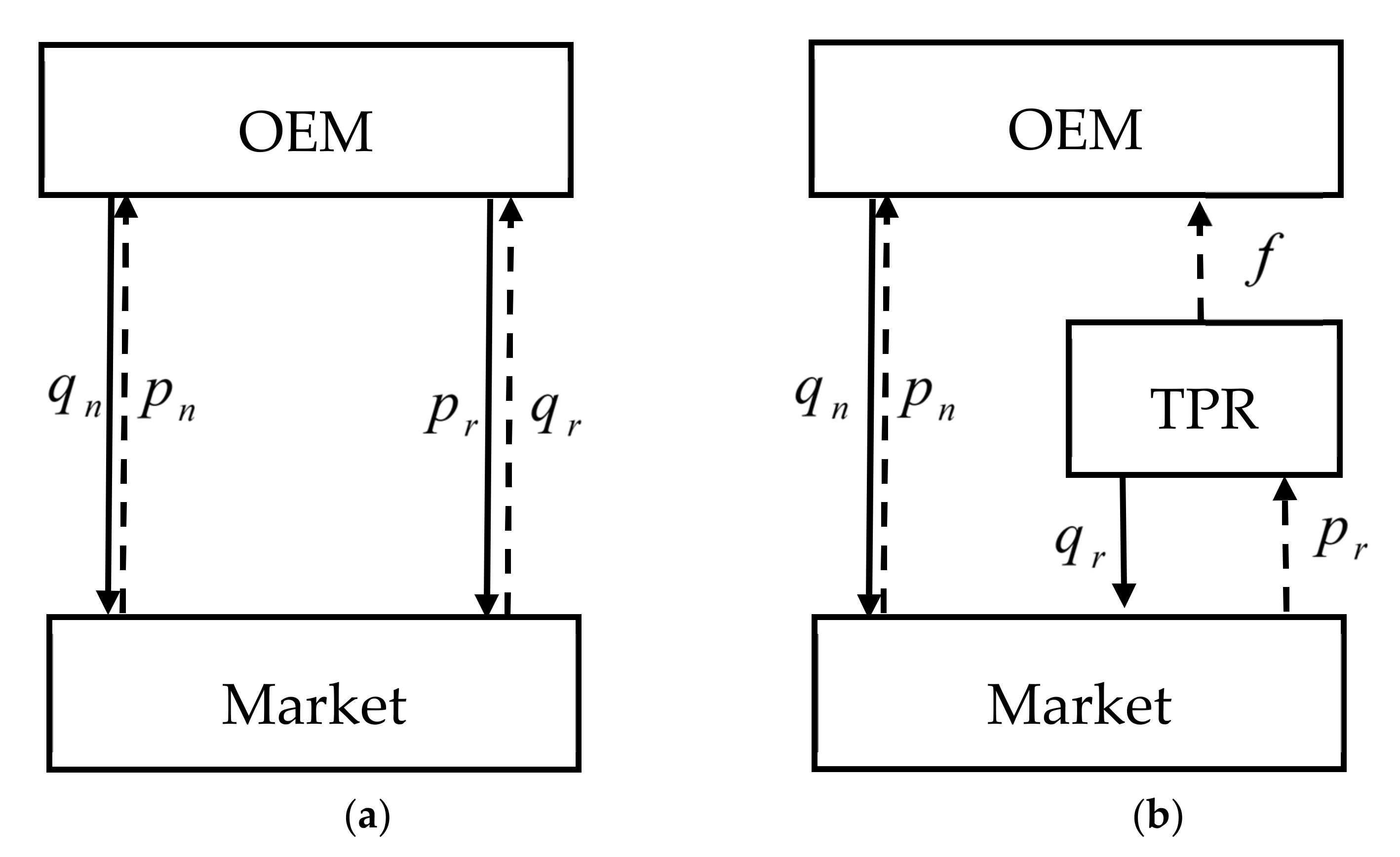
The primary goal of this paper is to explore how the economic, environmental, and social benefits of remanufacturing depend on the OEM’s strategic choice of interchangeable design, when remanufacturing is undertaken in-house or outsourced. As shown in Figure 1, under Model O, the OEM makes a strategic choice on design interchangeability, when the remanufacturing is conducted by itself. Model O is consistent with the fact that many OEMs have undertaken their remanufacturing operations in-house. For example, Canon, as one of the world’s largest remanufacturing operations, re-engaged in the interchangeable design of inkjet cartridges and launched remanufacturing programs for many years [25]. However, under Model T, the OEM only focuses on production and outsources the remanufacturing to TRPs. It should be noted that this model can illustrate how some OEMs, such as Apple, IBM, and Land Rover, have outsourced their remanufacturing operations to independent remanufacturers [26]. The details of assumptions made in this investigation will now be presented.
3.2. Model Assumptions
Assumption 1.
The interchangeability means that the products can be assembled and disassembled without force and results in a decrease in both the production and remanufacturing cost. That is, the per-unit cost for producing a new product isand the per-unit cost for remanufacturing is, whereis the spillover effect of interchangeability from the new product to the remanufactured product.
In this paper, the base unit manufacturing cost and the base unit remanufacturing cost are referred to as and , respectively. Since remanufacturing is always less costly than producing a new product [27], this study assumes that . This is consistent with the fact that remanufacturing costs over 40% less than new product manufacturing [28]. A product designed with a high interchangeability will be efficient for both assembling a new product and disassembling for remanufacturing, so the high interchangeability will directly decrease the production cost for both new and remanufactured products [4]. Let denote the OEM’s choice of interchangeability in their product design, which would result in the unit production cost of the new product being , and the unit remanufacturing product cost being , where is the spillover effect of interchangeability from the new product to the remanufactured product.
We assume that the interchangeable design induces a cost of , which is a quadric form of , where is the scaling parameter of with respect to . That is, we model the interchangeability levels, , as the function of the investment effort in product design, which is denoted by the cost of . To characterize the diminishing returns to investment, we use as a scaling parameter. Similar forms of response functions have been widely used in the quality choice in the remanufacturing context. For example, Wu [4] and Mukhopadhyay and Setoputro [29] investigated the sum of the additional costs associated with adjusting the design interchangeability. This paper investigates research issues that are similar to those in the above literature in the remanufacturing context.
Assumption 2.
Consumers are heterogeneous in their willingness to pay for new and remanufactured products. Each consumer value discount for the remanufactured products is a fraction () of the willingness to pay for the new products.
In this study, the mass of consumers is normalized to 1, and each consumer with their willingness to pay for a new product is assumed to be (). Consistent with the findings of previous studies [30,31], the primary consumer will discount the value of the remanufactured product so that it is a fraction () of the willingness-to-pay for a new product.
Based on the heterogeneity of consumers’ willingness to pay for new and remanufacturing products, we formulate that a customer can gain the net utility for a new product and per remanufactured unit. Therefore,
Assumption 3.
Both parties maximize their profits in a single-period model: the OEM first announces the level of interchangeability in product design () and the fees () charged for remanufacturing outsourcing. Then, both parties determine the optimal units of both products (i.e.,and).
The single-period model means that if all new products are deposited by the consumers, they can be returned for reuse immediately [26,32]. To keep this research focused, we consider the case that all used products are available for remanufacturing [33].
The related parameters and decision variables are provided in the following Table 2.
4. Model Formulation and Solution
In this section, we solve the optimal strategic decisions of both parties in a supply chain under two different models: Model O, in which both new and remanufactured products are made by the OEM, and Model T, where the OEM outsources the remanufacturing operations to the TPR.
4.1. Model O
In model O, the OEM first announces the degree of interchangeability in the product design (), and then chooses the optimal units of new and remanufactured products ( and ). The problem of the OEM can be given by
Equation (2) can be maximized with and . Then, by substituting and into the OEM’s profit, we can solve the optimal level of interchangeability in product design (the detailed decisions and profits can be found in Table 3).
4.2. Model T
Like model O, under model T, the OEM first determines the degree of interchangeability in the product design (), and the fees, , charged from remanufacturing outsourcing, simultaneously. Both parties’ profits can be maximized with and .
Therefore, the OEM’s problem and the TPR’s problem are as follows, respectively:
Then, we can obtain the optimal decisions under model T by adopting the backward approach again. All results are presented in Table 3.
To make sure that the sales of the new and remanufactured products are positive, and the demand for the new products is greater than that for remanufactured products, that is, , like Xiong et al. [31] and Zhang et al. [15], the following assumption should be imposed:
Assumption 4.
the unit remanufacturing cost () and the scaling parameter of the cost for interchangeability in product design () must satisfyand, respectively.
Assumption 4 means that, if the remanufacturing cost is too high, i.e., , the manufacturer or the independent remanufacturer would not remanufacture any used cores; that is . On the other hand, when the remanufacturing cost is too small, i.e., , the manufacturer would reluctant to offer enough new products for remanufacturing, that is, [15,31].
5. Model Analysis
We first focus on the equilibrium decisions of the two models, and then compare the differences in sustainability issues in the two models from economic, environmental, and social perspectives. Finally, we propose two possible remedies, including a revenue-sharing contract and subsidy-incentive mechanism, to achieve economic and environmental suitability for all parties (the proofs for all propositions are provided in Appendix A).
5.1. Comparison of Optimal Outcomes
This subsection highlights the difference in optimal outcomes, including the degree of interchangeability and the quantities of both products, between Model O and Model T. First, we analyze the degree of interchangeability as follows:
Proposition 1.
The OEM chooses the lower degree of interchangeability in Model T, that is,.
Proposition 1 suggests that when the remanufacturing is outsourced to the TPR, the OEM will decrease the degree of interchangeability in product design to reduce the cannibalization problem from remanufactured products. Note that a product designed with a high interchangeability will directly decrease the production cost and remanufacturing cost. Therefore, in Model O, the OEM intends to adopt a positive product design strategy with a high degree of interchangeability because both new and remanufactured products are offered by it. However, in Model T, all new products are produced by the OEM, but the remanufactured units are provided by the TPR. To deal with the fiercer competition from the TPR, the OEM chooses a low degree of interchangeability in product design, because the decrease in interchangeability can improve the difficulty of remanufacturing.
As Shu and Flowers [34] show, when the OEM and remanufacturer are not in direct competition with each other, the design for disassembly appears to be beneficial for the OEM. As such, Xerox undertakes the remanufacturing operations itself. Furthermore, Xerox has received much revenue in remanufacturing programmes due to the fact that it has heavily invested in interchangeable design to make its products easy to disassemble, and valuable when remanufactured [35]. However, if the OEM and remanufacturer are in direct competition, some OEMs may decrease the degree of disassembly to reduce the competition from remanufacturing. For instance, in the printer-cartridge industry, some OEMs, such as Hewlett–Packard Inc., try to limit the other remanufacturers by only producing single-use cartridges, which decreases the interchangeability of components [11,36]. Therefore, when facing great competition from remanufactured products, the OEM may adopt a product design with a low degree of interchangeability to increase the remanufacturer’s costs, thus weakening market cannibalization from remanufactured products.
The results of Liu et al. [37] also partly support Proposition 1. In particular, they conclude that the OEM takes a negative products design strategy if it does not engages in remanufacturing. However, it should be noted that this study is different form their research by considering the issue of interchangeable design in the remanufacturing outsourcing. Furthermore, as mentioned earlier, the results on interchangeable design that consider cannibalization problems between different product lines do not immediately extend to the interchangeable design involved in the remanufacturing context.
Proposition 2.
The optimal quantity of new products in Model T is lower than that of Model O, that is,. the opposite is true for the remanufactured products, that is,.
Proposition 2 indicates that when the TPR undertakes the remanufacturing operation, the OEM provides fewer units of new products, and the remanufacturer offers more units of remanufactured products. Firstly, according to proposition 1, in model O, the OEM provides a higher degree of interchangeability in product design, and both the production cost of new and remanufactured products can be reduced; That is, when the degree of interchangeability in product design is high, the cost savings for the new products are larger than the cost savings for the remanufactured products. As a result, the OEM has a more positive attitude towards the sales of new products than remanufacturing operations. Secondly, in Model T, as was mentioned before, all of the TPR’s profits are obtained from remanufacturing. Therefore, the TPR offers greater quantities of remanufactured products in Model T to maximize its own profit, which causes the number of units of new products to decrease.
5.2. Comparison of Economic Profitability
The OEM’s profitability is investigated as follows:
Proposition 3.
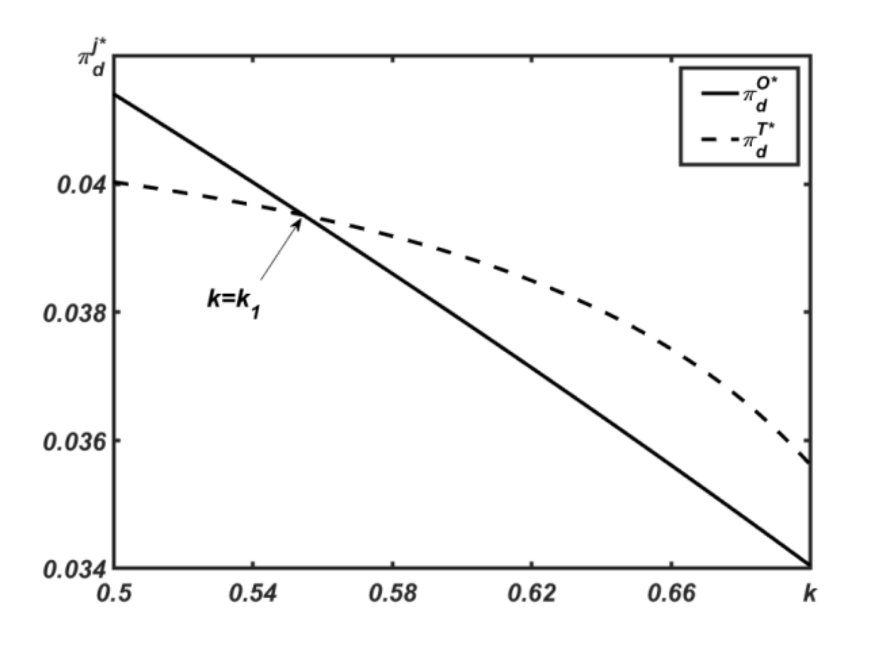
The OEM benefits less in model T than in model O; That is,.
Proposition 3 indicates that an OEM is always worse-off when remanufacturing operations are outsourced to the TPR. Before explaining Proposition 3, we briefly examine manufacturers’ profitability, which has two sources: (1) selling new products and (2) selling remanufactured products or charging TPR commission fees for remanufactured products. As mentioned earlier, in Model O, both products are provided by the OEM. However, in Model T, both products are provided by the OEM and TPR separately. Therefore, compared to Model O, the competition between new products and remanufacturing products is fiercer in Model T. The increased cannibalization from remanufactured products can decrease the OEM’s profits in two important ways. On the one hand, it causes the OEM to lower the degree of interchangeability in product design (see Proposition 1); That is, the decreasing interchangeability leads to an increase in the production costs of two products, particularly for the new products, which reduces the OEM to an increase new products. On the other hand, due to the direct cannibalization from the TPR’s remanufacturing, the quantities of new products decrease, while the opposite is true for the remanufactured products (see Proposition 2).
Although the OEM charges a fee for remanufactured products from the TPR, the benefits gained from remanufacturing under Model T are not so high that they can compensate for the loss from selling new products. Hence, the OEM is always worse off in model T. This may be consistent with the fact that some OEMs are willing to undertake the remanufacturing operations themselves and not outsource them to the authorized remanufacturers. For instance, Xerox has its own remanufacturing facilities in the USA, the UK, Japan, Australia, the Netherlands, Mexico, and Brazil; by undertaking remanufacturing operations itself, Xerox has saved millions of dollars in raw material and waste disposal costs and enhanced its image as an environmentally conscious company [35].
Extant studies have suggested that maximizing the industry always leaves impacts all parties the economic needs of all parties [38,39]. Therefore, we will further discuss the difference in the industry’s profitability predicted by the two models in the following proposition:
Proposition 4.
There exists a threshold, below which (i.e.,), the industry’s profitability in model T is lower than that in model O, that is,. Otherwise, the opposite is true, that is,.
Proposition 4 reveals that the scaling parameter of the cost for interchangeability in product design plays a strategic role in determining the industry’s profit in both models. In particular, when , the industry’s profit in model O is higher. In other words, when the scaling parameter of the cost for interchangeable design is relatively low (i.e., ), the industry would benefit more from the OEM’s monopoly position of providing both products, because it would maximize the profits from new products and remanufactured sales and limit the adverse effects of cannibalization problems. However, when the scaling parameter of the cost for interchangeability in product design is relatively high (i.e., ), this higher cost for interchangeable design is more harmful for Model O due to the fact that the OEM’s monopoly position is more sensitive to the variations in cost. In contrast, in Model T, new products are offered by the OEM, and remanufactured products are provided by the TPR separately. Therefore, compared to Model O, when , the competition between both parties breaks down the monopoly position of the OEM and provides a higher impetus for both parties to maximize their own profitability. Such competition naturally benefits the industry.
5.3. Comparison of Environmental Sustainability
Following the perspective on waste management of Agrawal et al. [40], this paper uses and to represent the per-unit disposal impacts of new and remanufactured products, respectively. Since the remanufacturing extends the new product lifecycle process and reduces waste disposal, the units obtained through remanufacturing have a lesser impact than that in new production; that is, > [41]. Then, the environmental impact can be calculated as , which can be concluded as follows:
Proposition 5.
Model T is always greener than Model O, that is,.
According to the equation , the environmental impact is not only related to the output of new products, but also to the quantity of remanufactured products. Based on the previous analysis, the quantities of new products provided by the OEM decrease (i.e., ), while the quantities of remanufactured products increase (i.e., ). This means that the resource saving from remanufacturing is greater, and the resource waste from new products is less in Model T.
Proposition 5 suggests that Model T is more environmentally friendly, due to the larger quantities of remanufactured and smaller quantities of new products produced under Model T. Therefore, from an environmental sustainability perspective, the OEM should be encouraged to outsource the remanufacturing operation. than Model O. However, if highlighting the OEM’s profitability, we find that the situations are quite different. That is, as Proposition 3 revealed, the OEM is always worse-off when remanufacturing operations are outsourced to the TPR. In sum, according to Proposition 3 and 5, we can conclude that, although Model T is more environmentally friendly, the OEM would not support the outsourcing of remanufacturing operations because this strategy always leaves the OEM worse off.
The argument is similar to the study of He et al. [42], who found that the OEM benefits more, but the environment is worse off when it determines the remanufacturing operation in-house. It should be noted that their study analyzes the economic and environment problems of remanufacturing outsourcing with focusing on the product quality choose; however, we examine how an OEM can use interchangeable design along with quantity as a competitive lever against the cannibalization problem from remanufacturing.
5.4. Comparison of the Social Performance
In this subsection, we study the differences in social welfare outcomes () between Model O and Model T; that is, this subsection focuses on how the impact of interchangeable design in remanufacturing processing will affect the social aspects of the participants in the supply chain.
Following the studies of Yenipazarli [43], this paper calculates the social welfare with a summary measure from three components: Consumer surplus; industry profit; and environmental cost:
- (1)
- Consumer surplus, , that is calculated as the following function:
- (2)
- ;
- (3)
- Industry’s profitability,, which has been discussed in Proposition 4;
- (4)
- The environmental cost of , where is the environmental impact discussed in Proposition 5, while represents a unit of emissions in a monetary unit, and [44].
Combining the components (1), (2), and (3), the total social welfare for model j is given as . As such, we compare the social welfare outcomes () of the two models in the following proposition:
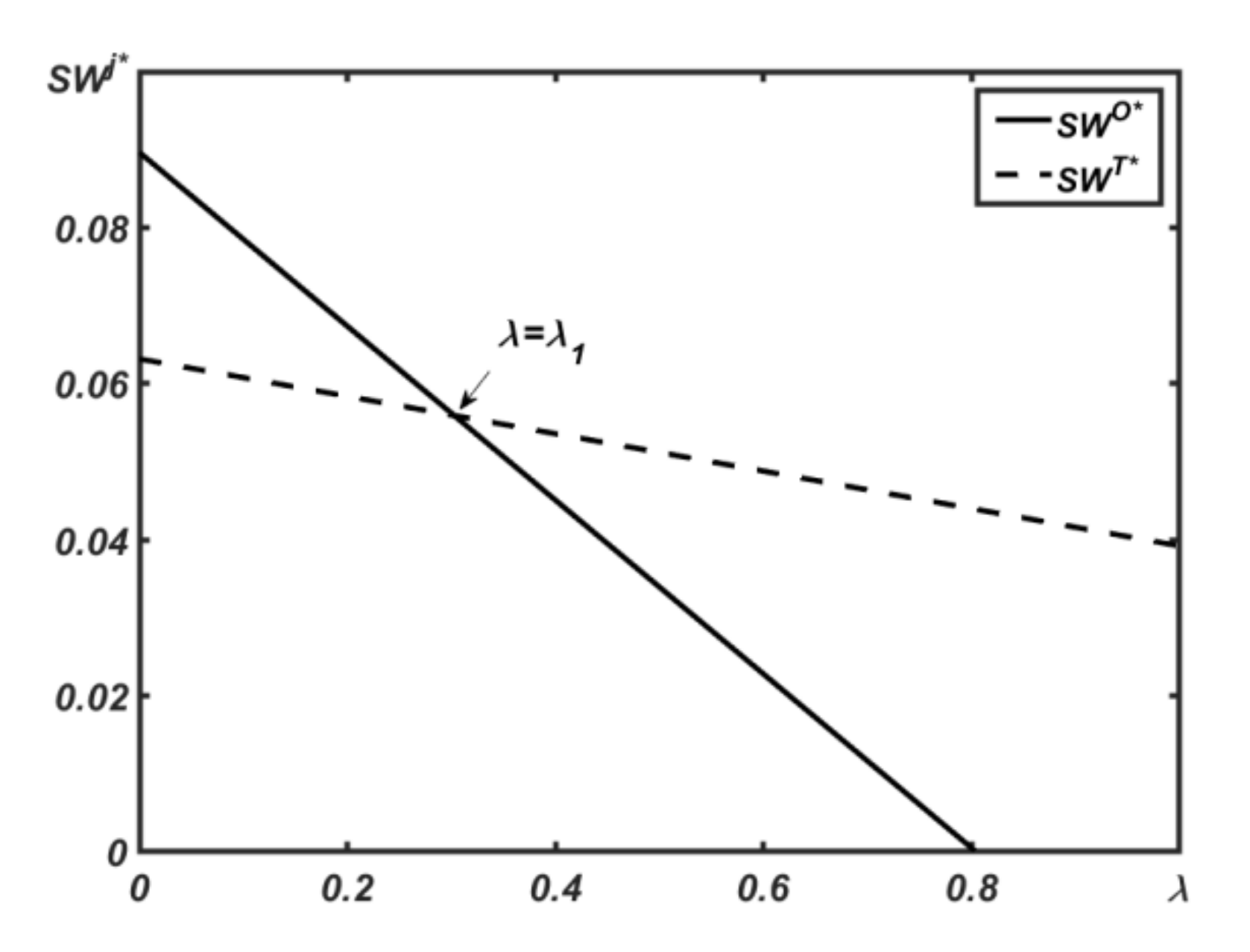
Proposition 6.
There exists a threshold, above which (i.e.,), the social welfare in Model T is larger than that in Model O, that is,. Otherwise, the opposite is true, that is,.
Proposition 6 reveals that, if the unit cost of emissions to the environment is pronounced, the social welfare in Model T is greater than that in Model O. Substituting the outcomes in Table 3 into , we can determine that the consumer surplus in Model T is lower than that in Model O due to the higher net utility and lower quantities of new products. Then, Proposition 6 can be explained by the consumer surplus and Propositions 4 and 5. Specifically, outsourcing remanufacturing to the TPR is not only always detrimental to the consumer surplus, but may also lead to a lower industry profit (see Proposition 4). However, Proposition 5 reveals that Model T is greener than Model O (see Proposition 5). As a result, as Proposition 6 shows, when the unit cost of emissions to the environment is higher, a smaller social welfare loss is perceived by the society in Model T due to environmental friendliness.
5.5. Two Remedies
Proposition 4 indicates that, when the scaling parameter of the cost for interchangeability in product design is relatively high, i.e., , the benefits to the TPR’s profitability in Model T are sufficient for “compensating” for OEM’s profit loss, and Proposition 5 further suggests that model T is more environmentally friendly than model O. As such, to fulfill the economic and environmental sustainability simultaneously, we need to take some measures to help both parties support Model T. More specifically, when , a revenue-sharing contract can be implemented to help all parties support Model T; however, if , to enable both parties to support Model T, a subsidy-incentive mechanism should be introduced.
5.5.1. A Revenue-Sharing Contract
Based on the results of Proposition 5, we find that, when , the TPR can undertake the remanufacturing outsourcing with the sharing parameter of (for Key parameters, see Table 4). Then, both parties are better off in model T, which is summarized in the following proposition:
Proposition 7.
When, compared to model O, the sharing parameter ofsatisfies the economic and environmental sustainability of Model T.
Proposition 7 suggests that, if , the OEM would prefer remanufacturing outsourcing. Additionally, if the sharing parameter of the revenue-sharing contract is , the TPR can benefit from remanufacturing and would like to produce remanufactured products. In sum, when , a revenue-sharing contract coordinates the benefit of both parties in Model T. Furthermore, such a contract not only has no impact on environmental requirements, but also makes the OEM better off in Model T.
We next introduce a subsidy-incentive mechanism that allows both parties to satisfy the economic and environmental sustainability. In practice, to promote the development of the remanufacturing industry and environmental sustainability, governments often provide subsidies. For example, the Chinese government offers a series of subsidies to customers who purchase the remanufactured products.
5.5.2. A Subsidy-Incentive Mechanism
Given that government subsidies are commonly provided in practice, in this subsection, we investigate the effect of subsidy incentives on the remanufacturing industry, and focus on the scenario where the government subsidizes the sales of remanufactured products under Model T. Specifically, the TPR will receive the per-unit subsidy for remanufactured products. Then, both parties’ optimization problems are as follows:
The superscript is denoted as the variables and results in Model T with the government subsidies. Comparing the results of Model T with the government subsidies with those of Model O, we propose a subsidy-incentive mechanism to benefit the OEM, and balance the economic and environmental requirements (for Key parameters, see Table 4).
Proposition 8.
When, the government can provide a subsidyfor each unit of remanufactured products in model T; furthermore, the OEM’s profit in model T would be larger than that in model O for.
On the one hand, Proposition 8 suggests that, for , the limited subsidy-incentive mechanism cannot create a “win-win” for both parties that satisfies the economic and environmental sustainability; That is, when , both parties can obtain revenue from the sales of remanufactured goods that allows both parties to be better off in model T, if the subsidiary parameter is not less than a certain amount, i.e., . Surprisingly, on the other hand, Proposition 8 further reveals that if , the subsidiary for remanufactured products is so high that the cannibalization problem from remanufacturing become fiercer, causing the OEM’s profitability to be decreased. Naturally, under this condition, the “win-win” would not increase, because the OEM would not support Model T.
6. Numerical Example
To gain a deeper understanding of the variations in the equilibrium outcomes between two modes, in this section, a numerical example is presented to reanalyze the above results.
Since the remanufacturing cost usually ranges from 25 to 75% of the manufacturing cost [45,46], this paper sets the parameters of the new production and remanufactured cost as and , respectively. Furthermore, as in [4], we denote the consumer value discount for remanufactured products and the cost savings parameter from the increasing degree of interchangeability as and , respectively. Consistent with Yan et al. [47], we set and , respectively.
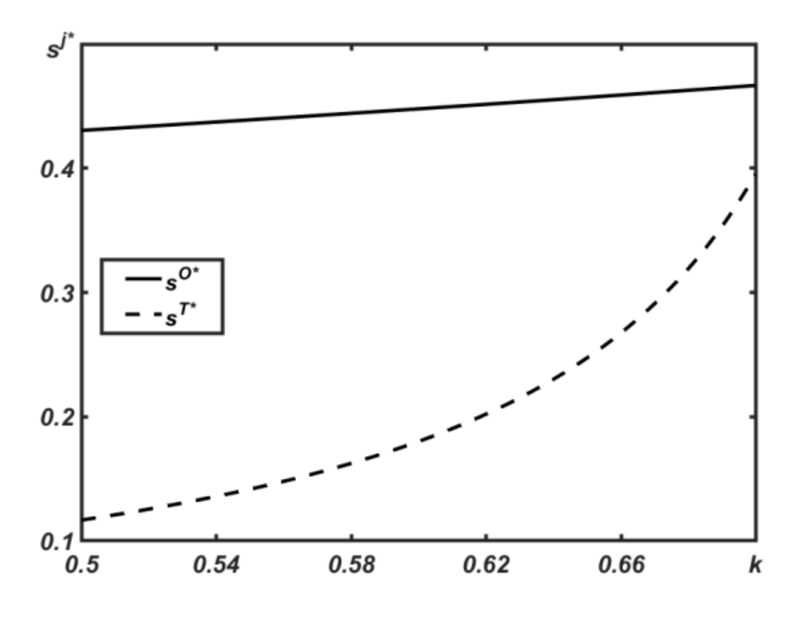
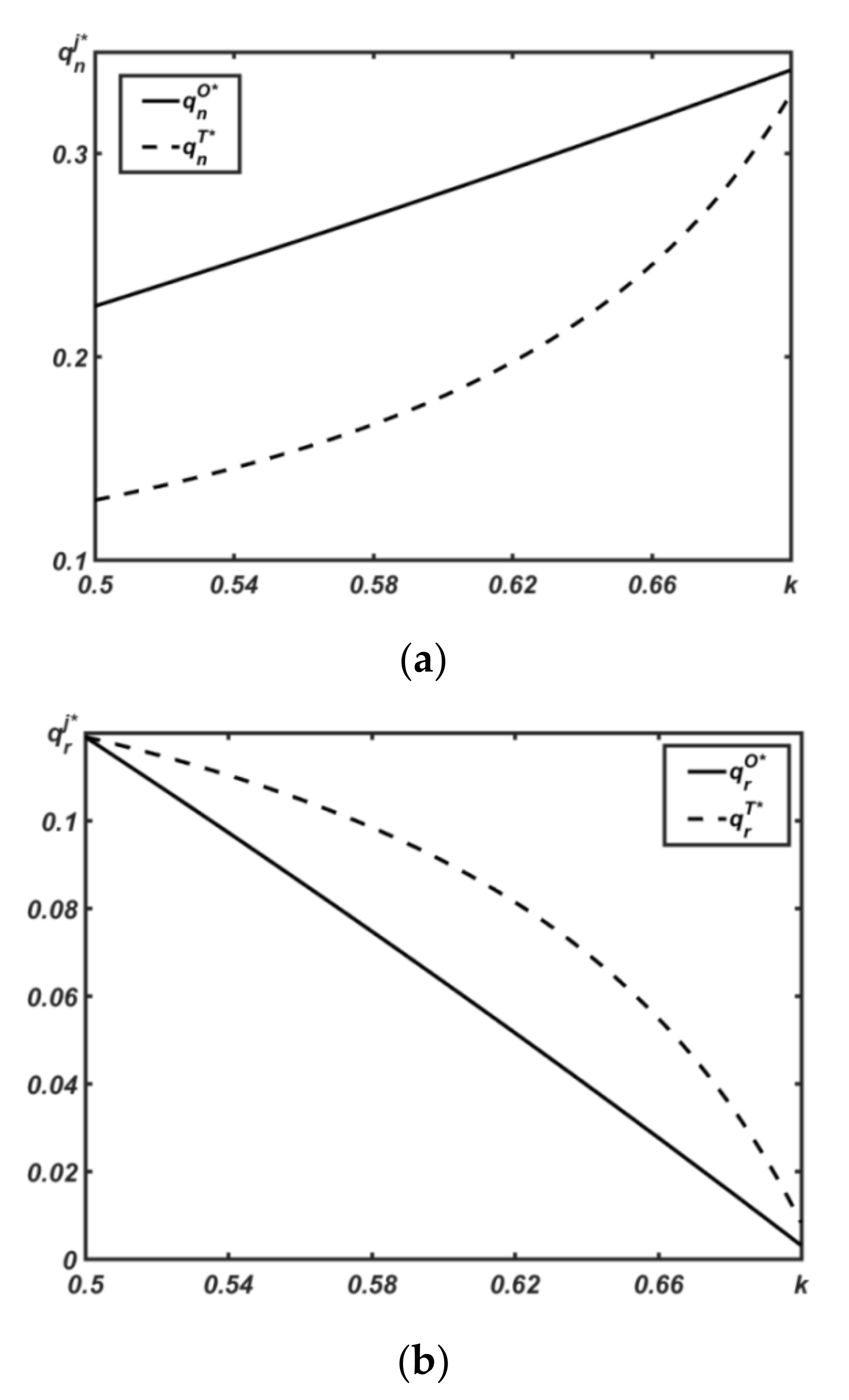
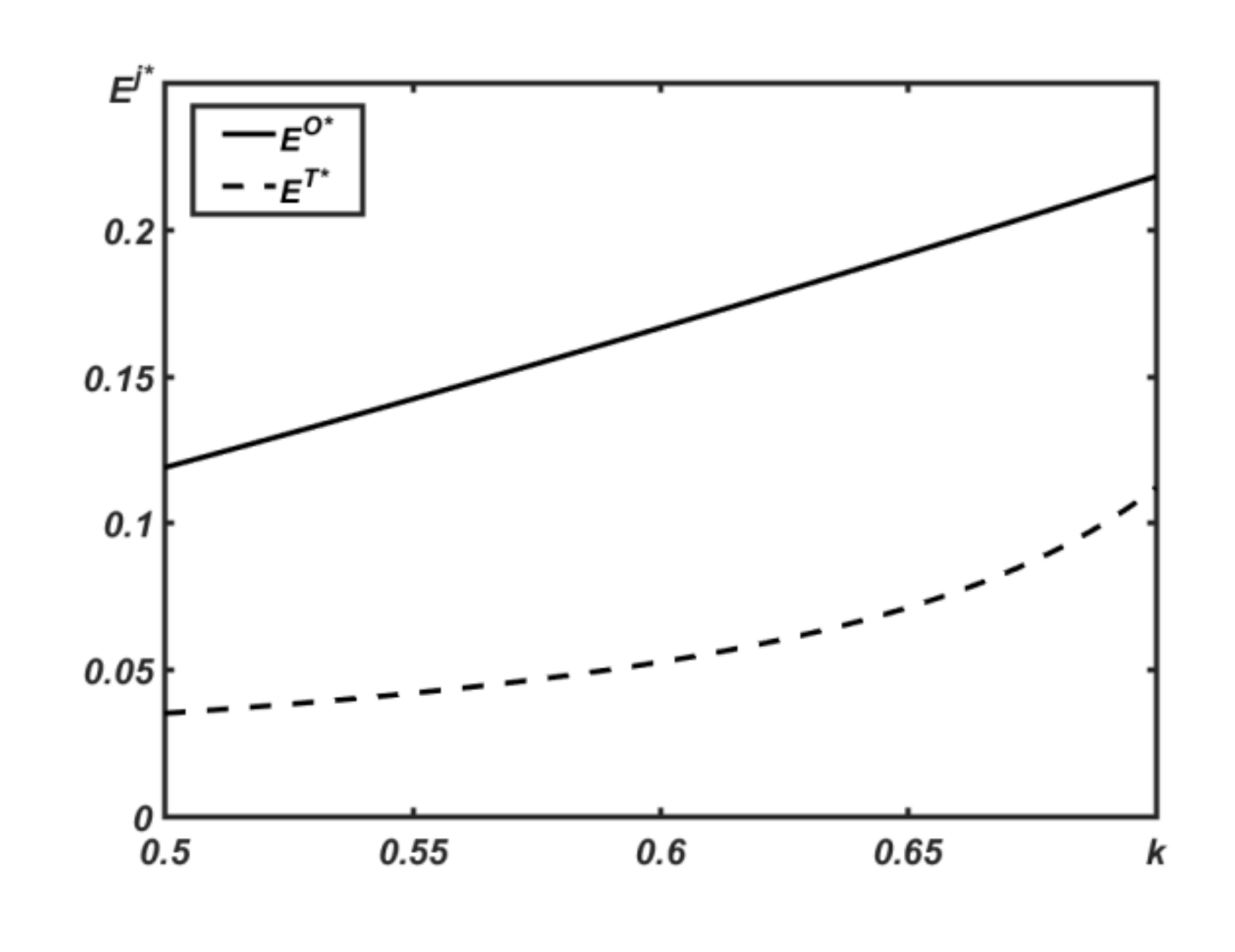
This subsection first presents a numerical simulation on the outcomes of optimal decisions, such as the interchangeable design and optimal quantities. From Figure 2, we can conclude that, consistent with Proposition 1, the OEM will choose a higher degree of interchangeability in Model O than in Model T (i.e., ). Furthermore, as the scaling parameter of the cost for interchangeability () increases, the difference in the levels in interchangeability between both models decreases. Next, the equilibrium quantities of new and remanufactured products are simulated in Figure 3. More specifically, according to Figure 3a, we can determine that ; That is, as Proposition 2 shows, the OEM tends to supply fewer quantities of new products in Model T than in Model O. Additionally, Figure 3b indicates that, as Proposition 2 shows, the equilibrium quantities of remanufactured products are higher in Model T than in Model O. In addition, we can further conclude that, as the scaling parameter of the cost for interchangeability increases (), the quantities of new products between both models increase, while the quantities of remanufactured products decrease.
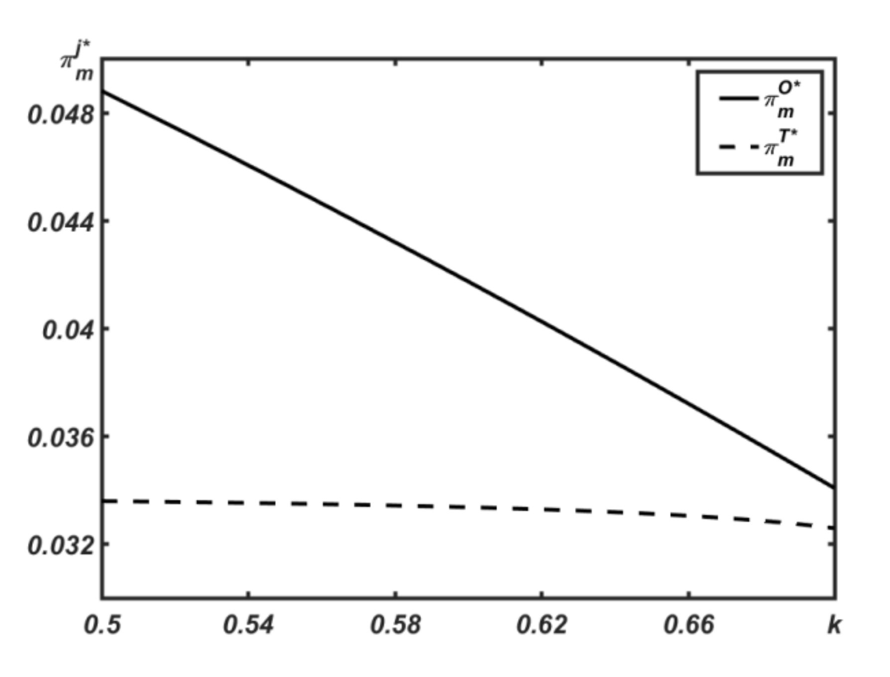
Then, Based on Figure 4, we can determine is always true. In addition, the difference in decreases with . Furthermore, as illustrated in Figure 5, we can find that there exists a threshold of , where the industry’s profits are higher in model T than those in model O (i.e., ), but are lower in Model O (i.e., ). This phenomenon is consistent with the theoretical argument discussed in Proposition 4.
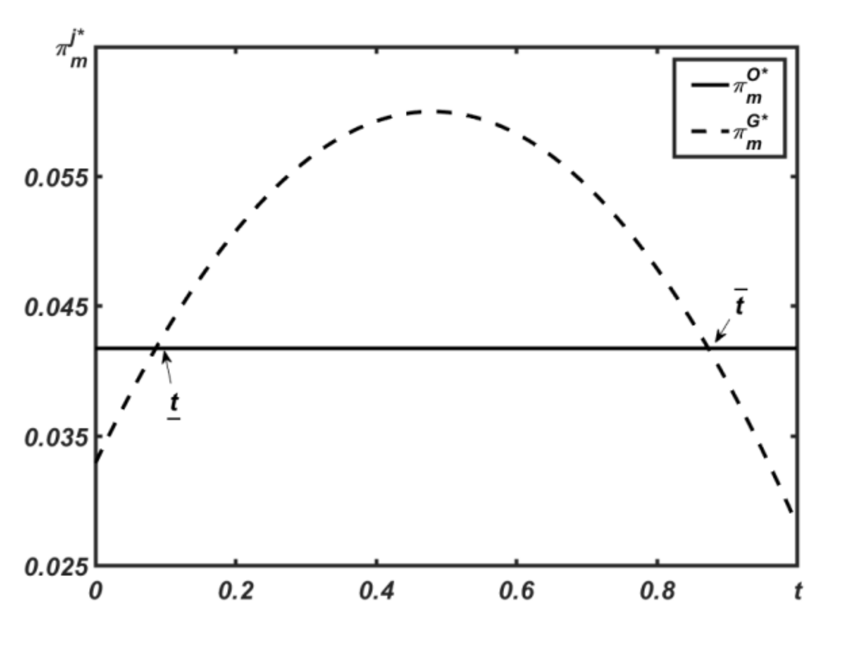
Figure 6 indicates that Model O will cause greater environmental impacts than Model T; that is, as Proposition 5 shows, Model T is always more environmentally friendly. Furthermore, the levels of environmental impact of both models increase with the scaling parameter of the cost for interchangeability. In addition, Figure 7 indicates that there also exists a threshold , where the social welfare is higher in Model T than that in Model O (i.e., ); otherwise, it is lower (i.e., ). Moreover, the higher the value of , the less social welfare due to environmental damage, which is illustrated by Figure 7.
Finally, Figure 8 and Figure 9 provide a numerical analysis on the two remedies. Specifically, Figure 8 indicates that, as Proposition 7 shows, when the scaling parameter of the cost for interchangeability in product design () is relatively high, the TPR would undertake remanufacturing outsourcing with ; if , the OEM would prefer to outsource the remanufacturing operation to the TPR. Additionally, if the sharing parameter of the revenue-sharing contract is , the TPR can benefit from remanufacturing and would like to produce remanufactured products. Figure 9 shows that, when the scaling parameter of the cost for interchangeability in product design () is low, a moderate government subsidy (i.e., ) can make both parties better in terms of remanufacting in-house. Figure 9 further reveals that, when the subsidiary parameter , the subsidy-incentive mechanism is too limited to create a “win-win” regarding the economic and environmental sustainability. However, if , the subsidiary for remanufactured products is so high that the cannibalization problem from remanufacturing becomes fiercer, causing the OEM’s profitability to be decreased; as such, the “win-win” also disappears.
We next conduct a sensitivity analysis to test the robustness of the above analytical results obtained in this paper. These sensitivity analysis results are summarized in Table 5 and Table 6.
First, as Table 5 and Table 6 show, in Model O and T, the optimal level of interchangeability in product design increases in . As the interchangeable design rises, the sales quantity of new products increases, while the demand for remanufactured products decreases.
Second, as summarized in Table 5 and Table 6, we observe that both the OEM and industry’s profits fall in . In particular, the profit decreases with a more gentle slope in Model T than Model O. For example, when the scaling parameter of the cost for interchangeability in products is increased from 0.50 to 0.68, the OEM’s profits in Model O and Model T are decreased by 36% and 32% respectively. Similarly, the industry’s profits in Model O and Model T are decreased by 36% and 14%, respectively. Moreover, based on Table 5 and Table 6, with increasing, the optimal industry’s profit may switch from remanufacturing in-house to remanufacturing outsourcing when is large enough (), which has been stated in Proposition 4.
Third, Table 5 and Table 6 also indicate that the consumer surplus, , and the environmental impacts, , increase with , while the social welfare, , decreases with it. Additionally, the social welfare decreases with a gentler slope in Model T than Model O. For example, when is increased from 0.50 to 0.58 and the unit cost of emissions to the environment , the social welfare in Model O and Model T is decreased by 20% and 11%, respectively. In particular, the optimal social welfare also depends on . When is high enough (), the social welfare in Model T is better off, and vice versa.
7. Conclusions, Implications, and Future Research Opportunities
Nowadays, interchangeable design is a quite common form in the process systems of various industries, such as automotive parts, electronics, furniture, and electrical appliances. Although the remanufactured products can cannibalize the new product sales, the interchangeable design can be efficient for both assembling for new production and disassembling for remanufacturing. As such, the interchangeable design confronted in remanufacturing processing often faces a balance of revenue from cost drivers and cannibalization effects from remanufacturing. The current literature has already explored the effect of product design between dependent products; however, their results do not immediately extend to the interchangeable design involved in the remanufacturing context.
In practice, in the remanufacturing context, many OEMs, such as Canon, Epson, and Xerox, have engaged in the interchangeable design of inkjet cartridges and launched remanufacturing programs for many years. However, other OEMs, including Apple, IBM, and Land Rover, have outsourced their remanufacturing operations to TPRs. Based on the observations of current practice, this paper develops two models where the OEM chooses the level of interchangeability in the product design, and has options of undertaking the remanufacturing operations itself (Model O), or outsourcing remanufacturing operations to TPRs (Model T). Using these two theoretical models, we investigate how the economic, environmental, and social benefits of remanufacturing depend on the OEM’s strategic choice of interchangeable design, when remanufacturing is undertaken in-house or outsourced.
We first found that, although the optimal level of interchangeability related to the product design in Model T is lower than that in Model O, the optimal quantity of remanufactured products under remanufacturing outsourcing is always higher than that in Model O. Conversely, although the OEM is always less likely to outsource its remanufacturing operations to independent remanufacturers, remanufacturing outsourcing may be more beneficial for the environment, industry, and society.
7.1. Research Implications
These findings of this research makes two main theoretical contributions to the literature. First, unlike the numerous literature highlighting the interchangeable design that considers cannibalization problems between high- and low-end products [13,14], the results of this paper focus on interchangeable design involved in the remanufacturing context. Second, in recent decades, whilst remanufacturing has gained much attention and been well studied from theoretical and empirical perspectives [15,16], this study provides insights on how the economic, environmental, and social benefits of remanufacturing depend on the OEM’s strategic choice of interchangeable design, when remanufacturing is undertaken in-house or outsourced.
7.2. Managerial Implications
From the managerial results, the above analysis reveals several important managerial insights for firms and environmental groups and agencies. In particular, for firms who have to make a strategic choice on design interchangeability, we have found that the outsourcing of remanufacturing actually deters the OEM’s strategic choice on design interchangeability. This is consistent with the fact that Lexmark makes its products less interchangeable to prevent remanufacturing from TPRs. Conversely, the latter key insight is relevant to environmental groups: Remanufacturing outsourcing may be more beneficial for the environment, industry, and society and depends on the OEM’s attitude towards its profitability loss. Furthermore, to eliminate the above contrasting effects between the OEM’s profitability and other issues, this study provides two possible remedies, such as a revenue-sharing contract and subsidy-incentive mechanism, to achieve a “win-win” situation.
7.3. Future Research Opportunities
In this paper, the models can be extended in the following ways. First, due to its tractability, we assumed that all decisions were considered in a single-period setting [4]. However, it worth addressing the relationship in multi-period models to highlight the product’s lifecycle. Second, to focus on the main research issues related to the effect of interchangeable design confronted in remanufacturing processing, this paper does not consider how the proposed mathematical formulation for product design can be integrated with product development technologies. However, Rashid et al. [48] and Rashid et al. [49] suggest that the product development technologies, particularly real-time optimization and economic control of production processes, can illustrate the improvement in economic performance under product design. As such, future researchers can extend models of this paper to address how the proposed mathematical formulation for product design can be integrated with product development technologies, such as real-time optimization and economic control of production processes. Finally, some of our assumptions, particularly the remanufacturing process without random defective, could be relaxed in future research. It should be note that the results may be different under a single-stage cleaner production system with random defective rate and remanufacturing.
Author Contributions
Writing and draft preparation, F.F.; writing—review and editing, S.C.; methodology—review and editing—origin, L.S. All authors have read and agreed to the published version of the manuscript.
Funding
This research was funded by National Natural Science Foundation of China (71672020, 72072020, and 71971043).
Institutional Review Board Statement
Not applicable.
Informed Consent Statement
Not applicable.
Data Availability Statement
Data is included in the paper.
Conflicts of Interest
We declare no conflict of interest.
Appendix A
This paper uses backward induction to solve for the equilibrium channel configuration. Thus, we solve the parameter scope of these nonlinear conditions in model O and T: , (referred to as , , , ). In the range of the threshold , for the rest of the paper, we compare the outcomes between Model O and Model T and draw the Proposition 1–8.
Appendix A.1. Proof for Proposition 1
To prove , we have to show that:
Let , we can obtain that in the range of the threshold , that is, the function is monotone increasing. Then solving , we can get , and . Thus, for any , the function is positive, that is to say, .
Appendix A.2. Proof for Proposition 2
(1) To prove , we have to show that:
Let , we can obtain that in the range of threshold , that is, the function is monotone increasing. Then solving , we can get , and . Thus, for any , the function is always positive, that is to say, .
(2) To prove , we have to show that:
Let , we can obtain that in the range of threshold , that is, the function is monotone decreasing. Then solving , we can get , and . Thus, for any , the function is negative, that is to say, .
Appendix A.3. Proof for Proposition 3
To prove , we have to show that:
Let , we can obtain that the function is convex, in the range of threshold . Further, solving , we get the only solution . Thus, the function is always positive, that is to say, . Hence, the OEM benefits less in model T than in model O.
Appendix A.4. Proof for Proposition 4
Comparing the whole industry’s profit between Model O and Model T, we give . Let , after simplification, that is:
Then, solving , we can get a threshold , when , , the function is convex. On the contrary, when , , the function is concave. Further, solving , we get the only solution . Thus, when , the function is positive, ie., . while , the function is negative, ie., , that is to say, the industry’s profitability in model T is higher than those in model O.
Appendix A.5. Proof for Proposition 5
Based on the analysis of Section 5.3, the disposal impact of new products can be referred as , the disposal impact of remanufactured products as . Thus, the total disposal impact in Model O and Model T are and . we can easily show that , because , , and . Thus, , meaning that the Model T is greener than Model O.
Appendix A.6. Proof for Proposition 6
Based on the analysis of Section 5.4, the difference of the social welfare between Model O and Model T, can be given as , according to this equation, we solve in the range of threshold , that is, the function is monotone decreasing. Further, solving , we can get
Thus, when , the function is negative, that is, , otherwise, if , the function is positive, that is, .
Appendix A.7. Proof for Proposition 7
When the scaling parameter of the cost for interchangeability in products design is relatively high, that is, , the industry’s profit in model T are higher than in model O, while the OEM’s profit is always worse off in model T. In such situation, TPR can share a portion of revenue to make the OEM support Model T, without hurt herself. Thus, we have to show that the OEM and the TPR’s profit should be better in Model T than that in Model O, that is, satisfy and .
To solve , we can show that . After simplification, we obtain.
That is to say, . Hence, when , for any , the OEM’s profitability in Model T would be higher than that in Model O.
To solve , we can obtain . That is to say, . Hence, when , for any ,the TPR’s profitability is always better in Model T.
Appendix A.8. Proof for Proposition 8
When the scaling parameter of the cost for interchangeability in products design is low, that is, , both of the industry and OEM’s profit in model T are less than in model O, while the environment is greener in model T than in model O. In this case, the government can provide a subsidy for per unit of remanufactured products to benefit the OEM, which can increase the industry simultaneously. Thus, we have to prove .
Let , we can obtain that the function is concave, i.e., for any in the range of threshold . Further, solving , we get the two solve:
and
Thus, when , the function is always positive, that is to say, . Hence, the OEM benefits better in model T than in model O, and prefer to support the model T.
References
- Tookanlou Parisa, B.; Wong Hartanto, W. Product line design with vertical and horizontal consumer heterogeneity: The effect of distribution channel structure on the optimal quality and customization levels. Eur. J. Market. 2020, 55, 95–131. [Google Scholar] [CrossRef]
- Miller, S. VW struggles with look-alike brands. Wall Street J. 1999, 1, M2. [Google Scholar]
- Caradvice. Toyota Has Unveiled a New Modular Global Vehicle Architecture That Will Underpin Approximately Half of All the Vehicles It Sells by 2020. 2015. Available online: https://www.caradvice.com.au/344812/toyota-reveals-new-modular-tnga-vehicle-architecture/ (accessed on 31 January 2021).
- Wu, C.-H. OEM product design in a price competition with remanufactured product. Omega 2013, 41, 287–298. [Google Scholar] [CrossRef]
- Desai, P.; Kekre, S.; Radhakrishnan, S.; Srinivasan, K. Product differentiation and commonality in design: Balancing revenue and cost drivers. Manag. Sci. 2001, 47, 37–51. [Google Scholar] [CrossRef]
- Jalali, H.; Carmen, R.; Van Nieuwenhuyse, I.; Boute, R. Quality and pricing decisions in production/inventory systems. Eur. J. Oper. Res. 2019, 272, 195–206. [Google Scholar] [CrossRef]
- Harivardhini, S.; Chakrabarti, A. A new model for estimating End-of-Life disassembly effort during early stages of product design. Clean Technol. Environ. Policy 2016, 18, 1585–1598. [Google Scholar] [CrossRef]
- Tripathi, V.; Weilerstein, K.; McLellan, L. Marketing Essentials: What Printer OEMs Must Do to Compete Against Low-Cost Remanufactured Supplies; Gartner Inc.: Stamford, CT, USA, 2009. [Google Scholar]
- Heese, H.S.; Swaminathan, J.M. Product Line Design with Component Commonality and Cost-Reduction Effort. Manuf. Serv. Oper. Manag. 2011, 8, 206–219. [Google Scholar] [CrossRef]
- Hauser, W.M.; Lund, R.T. The Remanufacturing Industry: Anatomy of a Giant: A View of Remanufacturing in America Based on a Comprehensive Survey across the Industry. Available online: www.bu.edu/reman (accessed on 2 February 2021).
- Wu, C.-H. Product-design and pricing strategies with remanufacturing. Eur. J. Oper. Res. 2012, 222, 204–215. [Google Scholar] [CrossRef]
- Oersdemir, A.; Kemahlioglu-Ziya, E.; Parlaktuerk, A.K. Competitive Quality Choice and Remanufacturing. Prod. Oper. Manag. 2014, 23, 48–64. [Google Scholar] [CrossRef]
- Afrin, K.; Nepal, B.; Monplaisir, L. A data-driven framework to new product demand prediction: Integrating product differentiation and transfer learning approach. Expert Syst. Appl. 2018, 108, 246–257. [Google Scholar] [CrossRef]
- Van den Broeke, M.M.; Boute, R.N.; Van Mieghem, J.A. Platform flexibility strategies: R&D investment versus production customization tradeoff. Eur. J. Oper. Res. 2018, 270, 475–486. [Google Scholar]
- Zhang, F.; Chen, H.; Xiong, Y.; Yan, W.; Liu, M. Managing collecting or remarketing channels: Different choice for cannibalisation in remanufacturing outsourcing. Int. J. Prod. Res. 2020, 1–16. [Google Scholar] [CrossRef]
- Geda, M.; Kwong, C.K. An MCMC based Bayesian inference approach to parameter estimation of distributed lag models for forecasting used product returns for remanufacturing. J. Remanufacturing 2021, 1–20. [Google Scholar] [CrossRef]
- Stanton, S.J.; Townsend, J.D.; Kang, W. Aesthetic responses to prototypicality and uniqueness of product design. Mark. Lett. 2016, 27, 235–246. [Google Scholar] [CrossRef]
- Joshi, Y.V.; Reibstein, D.J.; Zhang, Z.J. Turf Wars: Product Line Strategies in Competitive Markets. Mark. Sci. 2015, 35, 128–141. [Google Scholar] [CrossRef]
- Luchs, M.G.; Swan, K.S.; Creusen, M.E.H. Perspective: A Review of Marketing Research on Product Design with Directions for Future Research. J. Prod. Innov. Manag. 2016, 33, 320–341. [Google Scholar] [CrossRef]
- Majumder, P.; Groenevelt, H. Competition in Remanufacturing. Prod. Oper. Manag. 2010, 10, 125–141. [Google Scholar] [CrossRef]
- Shi, Z. Optimal remanufacturing and acquisition decisions in warranty service considering part obsolescence. Comput. Ind. Eng. 2019, 135, 766–779. [Google Scholar] [CrossRef]
- Li, K.; Li, Y.; Gu, Q.; Ingersoll, A. Joint effects of remanufacturing channel design and after-sales service pricing: An analytical study. Int. J. Prod. Res. 2019, 57, 1066–1081. [Google Scholar] [CrossRef]
- Han, X.; Shen, Y.; Bian, Y. Optimal recovery strategy of manufacturers: Remanufacturing products or recycling materials? Ann. Oper. Res. 2020, 290, 463–489. [Google Scholar] [CrossRef]
- Sun, L.; Zhang, L.; Li, Y. Sustainable Decisions on Product Upgrade Confrontations with Remanufacturing Operations. Sustainability 2018, 10, 4090. [Google Scholar] [CrossRef] [Green Version]
- Jixian. Canon Carrys out the Ink Cartridges’ Recycling: The Closed-Loop Recycling Program Promotes the Old Printer Cartridges’ Remanufacaturing. Available online: https://www.xianjichina.com/special/detail_471390.html (accessed on 2 February 2021).
- Zou, Z.-B.; Wang, J.-J.; Deng, G.-S.; Chen, H. Third-party remanufacturing mode selection: Outsourcing or authorization? Transp. Res. Pt. e-Logist. Transp. Rev. 2016, 87, 1–19. [Google Scholar] [CrossRef]
- Zhang, Y.; Chen, W. Optimal production and financing portfolio strategies for a capital-constrained closed-loop supply chain with OEM remanufacturing. J. Clean Prod. 2021, 279, 123467. [Google Scholar] [CrossRef]
- Giutini, R.; Gaudette, K. Remanufacturing: The next great opportunity for boosting US productivity. Bus. Horiz. 2003, 46, 41–48. [Google Scholar] [CrossRef]
- Mukhopadhyay, S.K.; Setoputro, R. Optimal return policy and modular design for build-to-order products. J. Oper. Manag. 2005, 23, 496–506. [Google Scholar] [CrossRef]
- Ma, P.; Gong, Y.; Mirchandani, P. Trade-in for remanufactured products: Pricing with double reference effects. Int. J. Prod. Econ. 2020, 230, 107800. [Google Scholar] [CrossRef]
- Xiong, Y.; Zhou, Y.; Li, G.; Chan, H.-K.; Xiong, Z. Don’t forget your supplier when remanufacturing. Eur. J. Oper. Res. 2013, 230, 15–25. [Google Scholar] [CrossRef] [Green Version]
- Galbreth, M.R.; Boyac, T.; Verter, V. Product reuse in innovative industries. Prod. Oper. Manag. 2013, 22, 1011–1033. [Google Scholar] [CrossRef]
- Reimann, M.; Xiong, Y.; Zhou, Y. Managing a closed-loop supply chain with process innovation for remanufacturing. Eur. J. Oper. Res. 2019, 276, 510–518. [Google Scholar] [CrossRef]
- Shu, L.; Flowers, W. A structured approach to design for remanufacture. In Proceedings of the 1993 ASME Winter Annual Meeting, New Orleans, LA, USA, 28 November–3 December 1993. [Google Scholar]
- Kerr, W.; Ryan, C. Eco-efficiency gains from remanufacturing: A case study of photocopier remanufacturing at Fuji Xerox Australia. J. Clean Prod. 2001, 9, 75–81. [Google Scholar] [CrossRef]
- HP Inc. Why HP Doesn’t Offer Remanufactured Print Cartridges. Available online: http://hp.sharedvue.net/sharedvue/resources/?rl=ipg-wp-no_reman_ink (accessed on 3 February 2021).
- Liu, Z.; Li, K.W.; Li, B.Y.; Huang, J.; Tang, J. Impact of product-design strategies on the operations of a closed-loop supply chain. Transp. Res. Pt. e-Logist. Transp. Rev. 2019, 124, 75–91. [Google Scholar] [CrossRef] [Green Version]
- Paolo, T.; Flavio, T.; Roberto, P. Performance measurement of sustainable supply chains: A literature review and a research agenda. Int. J. Product. Perform. Manag. 2013, 62, 782–804. [Google Scholar]
- Azevedo, S.G.; Carvalho, H.; Ferreira, L.M.; Matias, J.C.O. A proposed framework to assess upstream supply chain sustainability. Environ. Dev. Sustain. 2017, 19, 2253–2273. [Google Scholar] [CrossRef]
- Agrawal, V.; Ferguson, M.; Toktay, B.; Thomas, V. Is leasing greener than selling? Manag. Sci. 2012, 58, 523–533. [Google Scholar] [CrossRef] [Green Version]
- Geyer, R.; Van Wassenhove, L.; Atasu, A. The economics of remanufacturing under limited component durability and finite product life cycles. Manag. Sci. 2007, 53, 88–100. [Google Scholar] [CrossRef] [Green Version]
- He, W.; Liang, L.; Wang, K. Economic and Environmental Implications of Quality Choice under Remanufacturing Outsourcing. Sustainability 2020, 12, 874. [Google Scholar] [CrossRef] [Green Version]
- Yenipazarli, A. Managing new and remanufactured products to mitigate environmental damage under emissions regulation. Eur. J. Oper. Res. 2016, 249, 117–130. [Google Scholar] [CrossRef]
- Cachon, G.P. Retail Store Density and the Cost of Greenhouse Gas Emissions. Manag. Sci. 2014, 60, 1907–1925. [Google Scholar] [CrossRef] [Green Version]
- Esenduran, G.; Kemahlıoğlu-Ziya, E.; Swaminathan, J.M. Take-back legislation: Consequences for remanufacturing and environment. Decis. Sci. 2016, 47, 219–256. [Google Scholar] [CrossRef]
- Subramanian, R.; Subramanyam, R. Key Factors in the Market for Remanufactured Products. Manuf. Serv. Oper. Manag. 2012, 14, 315–326. [Google Scholar] [CrossRef] [Green Version]
- Yan, W.; Li, H.; Chai, J.; Qian, Z.; Chen, H. Owning or Outsourcing? Strategic Choice on Take-Back Operations for Third-Party Remanufacturing. Sustainability 2018, 10, 151. [Google Scholar] [CrossRef] [Green Version]
- Rashid, M.M.; Mhaskar, P.; Swartz, C.L.E. Handling multi-rate and missing data in variable duration economic model predictive control of batch processes. AICHE J. 2017, 63, 2705–2718. [Google Scholar] [CrossRef]
- Rashid, M.M.; Patel, N.; Mhaskar, P.; Swartz, C.L.E. Handling sensor faults in economic model predictive control of batch processes. AICHE J. 2019, 65, 617–628. [Google Scholar] [CrossRef]
Figure 1.
Two channel structures: (a) Model O and (b) Model T.

Figure 2.
Variations of .

Figure 3.
Variations of optimal of quantities: (a) variations of , and (b) variations of .

Figure 4.
Variations of .

Figure 5.
Variations of .

Figure 6.
Variations of .

Figure 7.
Variations of .

Figure 8.
The revenue-sharing contract.

Figure 9.
A subsidy-incentive mechanism.


Table 1.
Comparison of this study with related research.
| Author(s) | Interchangeable Design | Remanufacturing |
|---|---|---|
| Desai et al. [5], Stanton et al. [17], Joshi et al. [18], Afrin et al. [13] | √ | ✗ |
| Majumder and Groenevelt [20], Shi [21], Li et al. [22], Han et al. [23], Zhang et al. [15], Geda and Kwong [16] | ✗ | √ |
| This paper | √ | √ |
Table 2.
Definitions of the primary variables and decision variables.
| Type | Variable | Definition |
|---|---|---|
| Parameters | consumer willingness-to-pay for new products | |
| consumer value discount for remanufactured products | ||
| base unit production cost of new/remanufactured products | ||
| spillover effect of interchangeable design | ||
| scaling parameter of the cost for interchangeable design | ||
| unit environmental effect of a new/remanufactured product | ||
| player ’s profits under model | ||
| environmental effect under model | ||
| consumer surplus under model | ||
| social welfare under model | ||
| superscript, = m (OEM), 3p (TPR), d (Industry) | ||
| superscript, = O (Model O), T (Model T) | ||
| Decision variables | degree of interchangeability | |
| fees charged for remanufacturing outsourcing | ||
| production quantity of new/remanufactured products | ||
| price of new/remanufactured products |
Table 3.
Equilibrium decisions and profits.
| The OEM operates remanufacturing (Model O) |
| The TPR operates remanufacturing (Model T) |
Table 4.
Equilibrium decisions of two remedial measures.
| The key parameter of a revenue-sharing contract |
| The key parameter of a subsidy-incentive mechanism |
Table 5.
The sensitivity analysis results for Model O.
| 0.50 | 0.20 | 0.4673 | 0.2287 | 0.1206 | 0.0587 | 0.0566 | 0.0587 | 0.1459 | 0.0861 |
| 0.52 | 0.20 | 0.4710 | 0.2404 | 0.1118 | 0.0565 | 0.0571 | 0.0565 | 0.1588 | 0.0818 |
| 0.54 | 0.20 | 0.4747 | 0.2523 | 0.1000 | 0.0542 | 0.0575 | 0.0542 | 0.1719 | 0.0774 |
| 0.56 | 0.20 | 0.4785 | 0.2644 | 0.0880 | 0.0520 | 0.0580 | 0.0520 | 0.1851 | 0.0730 |
| 0.58 | 0.20 | 0.4823 | 0.2767 | 0.0758 | 0.0497 | 0.0586 | 0.0497 | 0.1986 | 0.0685 |
| 0.60 | 0.40 | 0.4862 | 0.2892 | 0.0634 | 0.0473 | 0.0591 | 0.0473 | 0.2123 | 0.0215 |
| 0.62 | 0.40 | 0.4902 | 0.3019 | 0.0508 | 0.0449 | 0.0597 | 0.0449 | 0.2262 | 0.0141 |
| 0.64 | 0.40 | 0.4942 | 0.3148 | 0.0380 | 0.0425 | 0.0603 | 0.0425 | 0.2404 | 0.0067 |
| 0.66 | 0.40 | 0.4983 | 0.3279 | 0.0250 | 0.0400 | 0.0610 | 0.0400 | 0.2548 | 0.0017 |
| 0.68 | 0.40 | 0.5025 | 0.3412 | 0.0118 | 0.0375 | 0.0617 | 0.0375 | 0.2694 | −0.0085 |
Table 6.
The sensitivity analysis results for Model T.
| 0.50 | 0.20 | 0.1531 | 0.1241 | 0.1225 | 0.0430 | 0.0272 | 0.0559 | 0.0622 | 0.0707 |
| 0.52 | 0.20 | 0.1860 | 0.1316 | 0.1194 | 0.0427 | 0.0281 | 0.0548 | 0.0695 | 0.0690 |
| 0.54 | 0.20 | 0.1783 | 0.1404 | 0.1147 | 0.0424 | 0.0291 | 0.0536 | 0.0780 | 0.0671 |
| 0.56 | 0.20 | 0.1943 | 0.1508 | 0.1091 | 0.0421 | 0.0304 | 0.0522 | 0.0879 | 0.0650 |
| 0.58 | 0.20 | 0.2134 | 0.1632 | 0.1024 | 0.0417 | 0.0320 | 0.0506 | 0.0998 | 0.0626 |
| 0.60 | 0.40 | 0.2367 | 0.1783 | 0.0942 | 0.0412 | 0.0340 | 0.0487 | 0.1144 | 0.0369 |
| 0.62 | 0.40 | 0.2657 | 0.1971 | 0.0841 | 0.0405 | 0.0365 | 0.0465 | 0.1325 | 0.0301 |
| 0.64 | 0.40 | 0.3028 | 0.2212 | 0.0711 | 0.0397 | 0.0400 | 0.0440 | 0.1556 | 0.0218 |
| 0.66 | 0.40 | 0.3519 | 0.2530 | 0.0539 | 0.0387 | 0.0449 | 0.0411 | 0.1862 | 0.0115 |
| 0.68 | 0.40 | 0.4201 | 0.2973 | 0.0301 | 0.0372 | 0.0522 | 0.0379 | 0.2288 | 0.0017 |
Publisher’s Note: MDPI stays neutral with regard to jurisdictional claims in published maps and institutional affiliations. |
© 2021 by the authors. Licensee MDPI, Basel, Switzerland. This article is an open access article distributed under the terms and conditions of the Creative Commons Attribution (CC BY) license (http://creativecommons.org/licenses/by/4.0/).
Share and Cite
MDPI and ACS Style
Fu, F.; Chen, S.; Sun, L. Revenue and Cannibalization: The Effect of Interchangeable Design Confronted Remanufacturing Processing. Processes 2021, 9, 497. https://0-doi-org.brum.beds.ac.uk/10.3390/pr9030497
AMA Style
Fu F, Chen S, Sun L. Revenue and Cannibalization: The Effect of Interchangeable Design Confronted Remanufacturing Processing. Processes. 2021; 9(3):497. https://0-doi-org.brum.beds.ac.uk/10.3390/pr9030497
Chicago/Turabian StyleFu, Feng, Shuangying Chen, and Lin Sun. 2021. "Revenue and Cannibalization: The Effect of Interchangeable Design Confronted Remanufacturing Processing" Processes 9, no. 3: 497. https://0-doi-org.brum.beds.ac.uk/10.3390/pr9030497
Note that from the first issue of 2016, this journal uses article numbers instead of page numbers. See further details here.