Modelling Methods and Validation Techniques for CFD Simulations of PEM Fuel Cells

Abstract

The large-scale adoption of fuel cells system for sustainable power generation will require the combined use of both multidimensional models and of dedicated testing techniques, in order to evolve the current technology beyond its present status. This requires an unprecedented understanding of concurrent and interacting fluid dynamics, material and electrochemical processes. In this review article, Polymer Electrolyte Membrane Fuel Cells (PEMFC) are analysed. In the first part, the most common approaches for multi-phase/multi-physics modelling are presented in their governing equations, inherent limitations and accurate materials characterisation for diffusion layers, membrane and catalyst layers. This provides a thorough overview of key aspects to be included in multidimensional CFD models. In the second part, advanced diagnostic techniques are surveyed, indicating testing practices to accurately characterise the cell operation. These can be used to validate models, complementing the conventional observation of the current–voltage curve with key operating parameters, thus defining a joint modelling/testing environment. The two sections complement each other in portraying a unified framework of interrelated physical/chemical processes, laying the foundation of a robust and complete understanding of PEMFC. This is needed to advance the current technology and to consciously use the ever-growing availability of computational resources in the next future.

1. Introduction

Nowadays, greenhouse gas emission reduction to keep global warming under control is the most urgent political target. According to the European climate policy, this means complete decarbonisation of the mobility sector by 2050, with several intermediate steps and emission targets [1,2]. While there is a strong trend to electrify passenger cars to fulfil future emission legislation, technical solutions for other mobility sectors, like long-haul transport, off-road applications, and air- and ship-traffic, are not straightforward [3]. The requirement of a high amount of stored onboard energy in conjunction with the weight and volume of current battery solutions necessitates research on alternatives.

Many European Union countries mention sustainable hydrogen production as an important solution to store and distribute the volatile excess energies from sun and wind power plants. Besides reformer processes based on the water–gas shift reaction, electrolysis of water is considered the most sustainable production path of “green” hydrogen as long as the energy supply is covered by CO${}_2$-free sources. The hydrogen can be used, on the one hand, for reconversion to electricity to overcome the “dark doldrums”, which designates phases of insufficient wind and sun exposure to stabilise the electric grid and, on the other hand, to act as an energy source for mobile applications.

The conversion of hydrogen’s chemical energy to mechanical energy can be realised with internal combustion engines or fuel cell/electric motor compounds. While the debate about which technology will prevail is still ongoing, the fuel cell solution has indisputable advantages in terms of conversion efficiency and local pollutant emissions. It is therefore considered a promising concept for mobile applications with high energy demands. The polymer electrolyte membrane fuel cells (PEMFCs) are particularly suitable due to their high power density, high efficiency and low operating temperatures. They consume hydrogen at the anode and oxygen from the air at the cathode and convert the chemical energy to electric power output. The product, and only exhaust, is pure water. The gases are distributed over the cell’s active area according to the flow field that is induced by the imprinted channel topology of the bipolar plates (BPP). The gases flow through the porous gas diffusion layer structures (GDLs) to the catalyst layers (CLs), where the electrochemical reactions occur. The electrolyte separates the anode and cathode compartments but enables the conduction of hydronium ions from the anode to the cathode. The polymer membrane needs to be hydrated to ensure proper conduction properties. Therefore, the water management of a low-temperature PEMFC is crucial for high performance. Sketches of a typical PEMFC assembly with its components and of the electrochemical reactions developing at CLs is reported in Figure 1a,b, respectively.

For the research and understanding of the processes happening inside of fuel cells, mathematical models were developed. Springer et al. [6] and Bernardi [7] developed the first 0D/1D mathematical models. In the following, more sophisticated 3D models were proposed to investigate the influence of liquid water [8]. Due to the continually increasing computational power, 3D-CFD simulations were successfully applied to fuel cell research during the last years. The CFD-simulation offers the possibility to analyse effects occurring inside a fuel cell with high spatial resolution, i.e., liquid water distribution, local species concentrations and the cell’s current distribution. However, the outcome of a typical CFD-model strongly relies on a huge number of material data and properties, which are usually unknown. The porosity and tortuosity of the GDL or the exchange current density of the cathode catalyst layer are just arbitrary examples to clarify the challenge. Therefore, assumptions must be made or sensitivity investigations must be carried out to gain the confidence of the model’s physical adherence.

The current work focuses on the modelling approaches for CFD simulation of PEM fuel cells and their validation. A short overview of electrochemistry is given in Section 2. In Section 3, the modelling methods of gas channels, GDLs, CLs and membrane can be found. Section 4 focuses on measurement techniques that are suitable to validate CFD models. First, the measurement methods to investigate the whole fuel cell stack are mentioned. In the second part of this section, the measurement techniques to obtain the most crucial material parameters with a significant impact on the overall solution are specified.

2. Electrochemistry

Fuel cells are energy conversion systems that convert the chemical energy of fuel into electrical energy via electrochemical reactions. This is obtained by the simultaneous development of two separate electrochemical reactions.

On the anode side, the hydrogen molecule reacts at the active sites of the anodic catalyst layer and separates into two electrons (e${}^{-}$) and two protons (H${}^{+}$), completing the Hydrogen Oxidation Reaction (HOR; Equation (1)). The electrons are driven by the potential gradient to the external circuit, originating the electric current useful to produce external work, while the protons migrate into the membrane (electrolyte) towards the cathode side. Here, the two H${}^{+}$ ions (from the membrane) and the two e${}^{-}$ from the external circuit react with the supplied oxygen molecule to form water and waste heat. This is the Oxygen Reduction Reaction (ORR; Equation (2)).

$${\mathrm{H}}_2⟶2{\mathrm{H}}^{\mathrm{+}}+{\mathrm{e}}^{\mathrm{-}}$$

(1)

$$\frac{1}{2}{\mathrm{O}}_2+2{\mathrm{H}}^{\mathrm{+}}+{\mathrm{e}}^{\mathrm{-}}⟶{\mathrm{H}}^2\mathrm{O}$$

(2)

Therefore, the overall reaction of the cell is the hydrogen oxidation (Equation (3)), for which the two half-reactions develop on the internal surface of the catalyst layers, separated by the electrolyte membrane.

$${\mathrm{H}}_2+\frac{1}{2}{\mathrm{O}}_2⟶{\mathrm{H}}^2\mathrm{O}$$

(3)

This is equivalent to the hydrogen combustion reaction where the heat released (enthalpy variation) is the heating value. However, a portion of this energy is not convertible into work due to the entropy production, leaving the variation of Gibbs free energy for useful work. The expression of the theoretical reversible cell potential $E_{rev}$ (Equation (4)) can be obtained from Gibbs free energy, entropy and temperature at reference conditions, and from the partial pressures of reactants/products. In an ideal case, this would be the cell potential regardless of the amount of produced current. However, in the real cases it represents the open circuit voltage (OCV) value, i.e., when no load is connected. When current is flowing, irreversible voltage losses are present (also known as overpotentials, related to activation, Ohmic and mass transfer losses) and their sum is known as the cell overpotential ${\eta }_{cell}$. The relationship between the cell voltage, the reversible voltage and the cell overpotential is given by Equation (5).

$$E_{rev}=\frac{G_{ref}}{2F}+\frac{S_{ref}}{2F}(T-T_{ref})+\frac{RT}{2F}ln\left(\frac{p_{H_2}{p}_{O_2}^{0.5}}{p_{H_{2}O}}\right)$$

(4)

$$E_{cell}=E_{rev}-{\eta }_{cell}$$

(5)

3. Modelling Methods for CFD Simulation of PEM Fuel Cells

3.1. Governing Equations

The governing equations for multidimensional PEMFC models express the general conservation principles common to any CFD simulation, i.e., conservation of mass, momentum, energy, species and charge. However, special modelling treatments dedicated to fuel cells are common to the most widespread models. These can be resumed in the following:

• Laminar: A common assumption in the numerical modelling of PEMFC is the consideration of laminar flows. This hypothesis is well justified by the typical velocity ranges in the gas channels (GC), with Reynolds number $Re\sim 1\times {10}^2$, further reduced in porous materials due to flow resistance.
• Steady State: The typical time-scales for PEMFC testing are in the order of minutes, thus justifying the assumption. For this reason, the governing equations presented in this paper are in the steady-state form. However, PEMFC testing cycles [9] and related transient simulations [10] are seeing a growing interest, as well as physical phenomena developing on relatively long time-scales ${\delta }_t$ (e.g., finite sorption rates with ${\delta }_t\sim$ 100–1000 s [11,12]).
• Multi-physics: All the models aiming at simulating processes in a PEMFC (or in a portion of it) include more than one component. Therefore, solid parts with different physics and macroscopic properties (e.g., GDL, CL and/or BPP) will be present alongside fluid continua, requiring dedicated modifications (source terms, material properties) to each equation.
• Multi-phase: Despite the fact that, in the following part of this section, a so-called single-phase approach will be presented, this is to be intended for fluid modelling in GC, GDL and CL. The dissolved water in the membrane (i.e., its presence in isolated clusters of molecules) is always accounted for, therefore introducing more than a single water phase in the simulation.
• Macro-homogeneous: All cell-scale models express the morphological/structural characteristics of solid parts via averaged (or effective) quantities, e.g., porosity, tortuosity, thermal/electrical conductivity, etc. With particular regard to porous parts (GDL and CL), the real fibrous structure is not directly modelled, and its effect is replaced by the use of calibrated integral properties. This allows great computational efficiency when simulating cell/stack domains.

In this context, a major role is played by the modelling of water and of its phase state, whose transport is a key trait for high-quality PEMFC 3D-CFD simulations. The interconnection between electrochemical kinetics, water content and liquid/vapour presence frames this sub-topic as a core problem. It involves all PEMFC parts (excluding solid BPP): CL are the production sites for H${}_2$O, porous GDL have the twofold task to remove waste H${}_2$O and delivering vapour H${}_2$O in humidified streams for adequate membrane hydration, the membrane hosts multiple water transport mechanisms (e.g., back-diffusion and electro-osmotic drag) and presents fundamental properties largely influenced by water content (e.g., ${\sigma }^{eff}$). In [5], the water states and the transport mechanisms for each component are exhaustively reviewed, presenting the different nature and their interconnection. In flow channels and porous materials (GDL and CL), water is transported via convection/diffusion mechanisms, with the additional complexity of its adherence to walls in porous materials. This is synthesised by the contact angle $\theta$, and hydrophobic materials ($\theta >90{}^{\circ }\mathrm{C}$) are preferred for lower transport losses. The effect is the presence of a capillary force, which can be seen as an additional momentum loss term, for which Leverett equations [13] are commonly used, although efforts for alternative formulations are proposed in [14,15].

The importance of water management is demonstrated by common PEMFC designs, e.g., the counterflowing anode/cathode streams are based on the desire to utilise the high water concentration at the cathode outlet to hydrate the membrane in the anode inlet proximity via water back-diffusion. Another example is the choice between straight-parallel and serpentine gas distributors [16], with the former excelling in reduced pressure losses for reactants delivery while the latter optimising water removal. Such designs are motivated by water handling issues; therefore, they testify the relevance of an accurate modelling of water management if 3D-CFD simulations are to be used alongside testing for design guidance of future PEMFC power systems [17,18,19].

In low-temperature PEMFC (conventionally operating between 60${}^{\circ }\mathrm{C}$–80${}^{\circ }\mathrm{C}$ at ambient or minimally pressurised levels), water condensation is always possible. From a numerical point of view, the presence of a multi-phase fluid implies the need for an adequate modelling approach. Conversely, the ease of water management is one of the main favourable aspects of the High-Temperature PEMFC (HT-PEMFC; operating $T>100 {}^{\circ }\mathrm{C}$), for which water is only present in single-phase gaseous form [20,21,22,23].

In the next paragraphs, the most common techniques are grouped and described (MMP, EMP and VOF). Another possible grouping for water management models is presented in [24], identifying (I) models aiming at simulating the water transport within the membrane [6,25], (II) cell-scale CFD models assuming a uniform membrane water content (e.g., fully hydrated) and (III) comprehensive models combining the previous two categories to provide a cell-scale representation of water transport including membrane/CL phenomena.

Alongside these approaches, mainly dealing with fluid treatment and water phase management, ionomer specific transport mechanisms are present at CL and membrane, i.e., electro-osmotic drag (from anode to cathode), back-diffusion and hydraulic permeation (from cathode to anode). Their relevance cannot be underemphasised as water concentration is a promoter of H${}^{+}$ transport (hence increasing the charge conductivity) via vehicular/hopping mechanisms. Wu et al. [26] compared several approaches for water transport and formation in a non-isothermal single straight-channel H${}_2$/air 3D-CFD model. They pointed out that water is formed in a dissolved phase at the CCL and that its evolution into a liquid water phase depends closely on the degree of saturation of the surrounding cathode gas stream.

3.1.1. Mixture Multi-Phase (MMP)

The Mixture Multi-Phase model (MMP) method assumes that the two fluid phases are miscible and at equilibrium, and their motion can be simulated as that of a unique continuum. This corresponds to an eulerian representation of low-saturated streams where isolated liquid droplets are transported by the bulk flow. This simplification implies that a single continuity, momentum and energy equation is solved for the eulerian mixture, and the phases subdivision (sharing the same mixture velocity ${\overrightarrow{u}}_{mix}$) is handled by a dedicated transport equation for the volume fraction and the phase relative velocity, or postprocessed via thermodynamic values (e.g., saturation tables).

The governing equations for the single-phase/MMP model are reported in

Table 1. Steady-state form of the mixture multi-phase (MMP) governing equations from [5,24].

	Equation
Mass	$\nabla \left({\rho }_{mix}{\overrightarrow{u}}_{mix}\right) =S_m$
Momentum	$\nabla \left(\frac{{\rho }_{mix}{\overrightarrow{u}}_{mix}{\overrightarrow{u}}_{mix}}{{ϵ}^2}\right)=-\nabla p+\mu \nabla \left[\nabla \left(\frac{{\overrightarrow{u}}_{mix}}{ϵ}\right)+\nabla \left(\frac{{\overrightarrow{u}}_{mix}^T}{ϵ}\right)\right]-\frac{2}{3}\mu \nabla \left[\left(\frac{{\overrightarrow{u}}_{mix}}{ϵ}\right)\right]+ S_u$
Species	$\nabla \left({\rho }_{mix}{Y}_i{\overrightarrow{u}}_{mix}\right)=\nabla (\rho D_i^{eff}\nabla Y_i)+S_i$
Energy	$\nabla \left[{\left({\rho }_{mix}{c}_p\right)}^{eff}{\overrightarrow{u}}_{mix}T\right]=\nabla \left(k^{eff}\nabla T\right)+ S_T$
Charge	$\nabla \left({\kappa }^{eff}\nabla {\Phi }_s\right) + S_{{\Phi }_s}=0$
	$\nabla \left({\sigma }^{eff}\nabla {\Phi }_e\right) + S_{{\Phi }_e}=0$

in steady-state form, and the related source terms are listed in

Table 2. Source terms for the mixture multi-phase (MMP) governing equations from in [5,24].

	GC	GDL	CL	Solid Parts
Mass	$S_m=0$	$S_m=0$	$S_m={\sum }_i{S}_i$	${\overrightarrow{u}}_{mix}=0$
Momentum	$ϵ=0$	$S_u=\left(-\frac{\mu }{K_{GDL}}\right){\overrightarrow{u}}_{mix}$	$S_u=\left(-\frac{\mu }{K_{CL}}\right){\overrightarrow{u}}_{mix}$	${\overrightarrow{u}}_{mix}=0$
	$S_u=0$
Species	$S_i=0$	$S_i=0$	Anode H${}_2$: $S_{H_2,a}=-\frac{j_a}{2F}{M}_{H_2}$	$Y_i=0$
			Anode H${}_2$O:
			$S_{H_{2}O,a}=-\nabla \left[\frac{n_d}{F}{\sigma }_{eff}\nabla {\Phi }_e\right]M_{H_{2}O}$
			Cathode O${}_2$: $S_{O_2,c}=-\frac{j_c}{4F}{M}_{O_2}$
			Cathode H${}_2$O:
			$S_{H_{2}O,c}=\frac{j_c}{2F}{M}_{H_{2}O}+\nabla \left[\frac{n_d}{F}{\sigma }_{eff}\nabla {\Phi }_e\right]M_{H_{2}O}$
Energy	$S_T=0$	$S_T=\frac{i_s^2}{{\kappa }^{eff}}$	Anode CL:	BPP:
			$S_T=j_a\left|{\eta }_{act}\right|+\frac{i_s^2}{{\kappa }^{eff}}+\frac{i_e^2}{{\sigma }^{eff})}$	$S_T=\frac{i_s^2}{{\kappa }^{eff}}$
			Cathode CL:	Membrane:
			$S_T=j_c\left|{\eta }_{act}\right|+\frac{j_{c}T\Delta S}{2F}+\frac{i_s^2}{{\kappa }^{eff}}+\frac{i_e^2}{{\sigma }^{eff}}$	$S_T=\frac{i_e^2}{{\sigma }^{eff}}$
Charge	${\Phi }_s=0$	$S_{{\Phi }_s}=0$	Anode CL: $S_{{\Phi }_s}=-j_a,S_{{\Phi }_e}=j_a$	$S_{{\Phi }_s}=0$
	${\Phi }_e=0$	$S_{{\Phi }_e}=0$	Cathode CL: $S_{{\Phi }_s}=j_c,S_{{\Phi }_e}=-j_c$	$S_{{\Phi }_e}=0$

.

The single-phase/MMP method represents the simplest comprehensive equation set to model the conservation and transport principles present in PEMFC, and it has largely contributed to the development of CFD in PEMFC [24,27]. In addition to the mentioned mixture fluid assumption, a further convenience of the single-phase/MMP equations is their application to all the domains present in PEMFC, with only part-specific modifications (e.g., source terms), thus rendering it a simple, unified and consistent model in terms of intra-component fluxes.

The main hypothesis of the presented framework is the allowance of a single fluid phase at equilibrium, i.e., liquid water is bundled in an averaged mixture fluid and not separately transported. This implies allowing saturation values higher than unity (supersaturation) to represent a vapour–liquid mist mixture of equal velocity (${\overrightarrow{u}}_{mix}$), with evident ease of implementation. The single-phase/MMP method is largely used in 3D-CFD simulations of PEMFC [28,29,30], although it preserves adherence to physics only for low saturation levels. For high saturated conditions, not only the physical soundness is questioned, but also numerical issues arise due to the mass-averaging of phases of largely different densities (gaseous/liquid) in the momentum equation.

The mass conservation (or continuity) equation in Table 1 can be ubiquitously solved if (I) in solid parts ${\overrightarrow{u}}_{mix}=0$ is imposed and (II) in CL the source term ($S_m$, Table 2) accounts for the local creation/destruction of all species operated by electrochemical reactions and by the the net water transport across the polymeric membrane.

The momentum conservation equation inherits the $ϵ=0$ (in GC) and ${\overrightarrow{u}}_{mix}=0$ (for solid parts) specification, while showing dedicated $S_u$ in porous GDL and CL. In this context, they are commonly used to replicate the viscous and inertial contributions to flow resistance expressed by the Darcy–Forchheimer law [13]. Capillary effects can be added as additional momentum sources.

The steady-state species conservation equation for the mass fraction $Y_i$ of the i-th substance is expressed by a conventional advection–diffusion equation. It is applied without modifications in GC, GDL and solid parts, where no source terms are considered ($S_i=0$). However, $S_i$ is proportional to the local volumetric current density $j_{a/c}$ in CL for reactants/products (H${}_2$ at anode, O${}_2$ and H${}_2$O at cathode), and the contribution of electro-osmotic driven diffusion in included $S_{H_{2}O,a/c}$. An important addendum to the MMP method is that water is created/consumed from the single-phase fluid mixture, i.e., there is no specification of the actual water phase in electrochemical reactions (dissolved), as it will be specified in Section 3.5.

The species diffusion term $D_i^{eff}$ is the conventional gaseous diffusion coefficient $D_i$ in gas channels, which is usually experimentally measured at reference conditions ($D_{i,0}$) and extrapolated to operating pressure and temperature as in Equation (6):

$$D_i(T,p)=D_{i,0}{\left(\frac{T}{T_0}\right)}^{1.5}\left(\frac{p_0}{p}\right)$$

(6)

The reference values for diffusion coefficients in [${\mathrm{m}}^2/\mathrm{s}$] at reference conditions ($T_0=353\mathrm{K}$, $p_0=1\mathrm{atm}$) are $D_{H_2,0}=1.1\times {10}^{-4}$, $D_{O_2,0}=3.2\times {10}^{-5}$ and $D_{H_{2}O,0}=7.35\times {10}^{-5}$. The effect of the material porosity on the species diffusion is accounted for by the Bruggeman correction [31], changing $D_{i,0}$ into $D_{i,0}^{\ast }$ as in Equation (7).

$$D_{i,0}^{\ast }=D_{i,0}·{ϵ}^{1.5}$$

(7)

However, in porous regions the Knudsen diffusion has to be considered alongside the molecular one, as the pore size for the fluid becomes comparable to the molecular mean free path. This is especially verified in the ultra-small pores of CL. The gas kinetic theory expresses the Knudsen diffusion coefficient $D_{i,K}$ as a function of the pore radius $r_p$ as in Equation (8):

$$D_{i,K}=\frac{2}{3}{\left(\frac{8RT}{\pi M_i}\right)}^{0.5}{r}_p$$

(8)

Therefore, the generic form of the effective diffusion coefficient $D_i^{eff}$ in Equation (9) includes both mechanisms:

$$D_i^{eff}={\left(\frac{1}{D_i}+\frac{1}{D_{i,K}}\right)}^{-1}$$

(9)

The steady-state form of the energy equation considers the heat capacitance $\rho c_p$ of the material, which is modified into an effective heat capacitance ${\left(\rho c_p\right)}^{eff}$ for porous media including the solid phase heat capacitance ${\left(\rho c_p\right)}_s$ as in Equation (10). Heat generation via the Joule effect is localised in all the electric conductive components (GDL, CL and membrane), with an additional electrochemical reaction heating contribution for CL.

$${\left(\rho c_p\right)}^{eff}=ϵ\left(\rho c_p\right)+(1-ϵ){\left(\rho c_p\right)}_s$$

(10)

The charge transport equation is divided into electrodes (s) and electrolyte (e) forms, considering the effective electrical and ionic (protonic) conductivity (${\kappa }^{eff}$ and ${\sigma }^{eff}$, respectively), and a potential source term $S_{{\Phi }_{s/e}}$ modified only in the CL where electrochemical reactions develop. The volumetric electric current density j [$\mathrm{A}/{\mathrm{m}}^3$] is typically calculated using Butler–Volmer kinetics equations, as it will be discussed in Section 3.5. Charge transport is prevented in fluid regions, acting as insulators (${\Phi }_{s/e}=0$), while materials for GDL and electrodes are excellent conductors. The use of the $eff$ superscript refers to the macrohomogeneous approach for solid parts modelling, e.g., the porous and fibrous nature of GDL leads to an effective conductivity (${\kappa }_s^{eff}$) different in value and in direction dependence than the solid material one (${\kappa }_s$). A number of pioneering multidimensional CFD models for PEMFC rely in one form or another on this set of single-phase equations, such as in [32,33].

3.1.2. Eulerian Multi-Phase (EMP)

In the Eulerian Multi-Phase (EMP) model the two phases are independently transported via specific continuity, momentum and energy equations, and inter-phase closure is provided. For this reason, it is also named a two-fluid model. The number of equations makes the EMP method numerically expensive, although it preserves the highest adherence to highly saturated physical states. The governing equations for the EMP model are reported in

Table 3. Steady-state form of the eulerian multi-phase (EMP) governing equations from the works in [5,24].

	Equation
Mass (gas)	$\nabla \left({\rho }_g{\overrightarrow{u}}_g\right)=S_m$
Momentum (gas)	$\nabla \left(\frac{{\rho }_g{\overrightarrow{u}}_g{\overrightarrow{u}}_g}{{ϵ}^2{(1-{\alpha }_l)}^2}\right)=-\nabla p_g+{\mu }_g\nabla \left[\nabla \left(\frac{{\overrightarrow{u}}_g}{ϵ(1-{\alpha }_l)}\right)+\nabla \left(\frac{{\overrightarrow{u}}_g^T}{ϵ(1-{\alpha }_l)}\right)\right]-\frac{2}{3}{\mu }_g\nabla \left[\left(\frac{{\overrightarrow{u}}_g}{ϵ(1-{\alpha }_l)}\right)\right]+S_u$
Species (gas)	${\displaystyle \nabla \left({\rho }_g{Y}_i{\overrightarrow{u}}_g\right)=\nabla ({\rho }_g{D}_i^{eff}\nabla Y_i)+S_i}$
Water (liquid)	$\nabla \left({\rho }_l{\overrightarrow{u}}_l\right)=\nabla ({\rho }_l{D}_l\nabla {\alpha }_l)+S_l$
Energy (gas)	$\nabla \left[{\left({\rho }_g{c}_{p,g}\right)}^{eff}{\overrightarrow{u}}_g{T}_g\right]=\nabla \left(k_g^{eff}\nabla T_g\right)+S_{T,g}$
Energy (liquid)	$\nabla \left[{\left({\rho }_l{c}_{p,l}\right)}^{eff}{\overrightarrow{u}}_l{T}_l\right]=\nabla \left(k_l^{eff}\nabla T_l\right)+S_{T,l}$)

in steady-state form, and the related source terms are in

Table 4. Source terms for the eulerian multi-phase (EMP) governing equations from the works in [5,24].

	GC	GDL	CL
Mass (gas)	$S_m=-S_{gl}$	$S_m=-S_{gl}$	$S_m=-S_{gl}+{\sum }_i{S}_i$
Momentum (gas)	$ϵ=0$	$S_u=\left(-\frac{{\mu }_g}{K_{GDL}}\right){\overrightarrow{u}}_g$	$S_u=\left(-\frac{{\mu }_g}{K_{CL}}\right){\overrightarrow{u}}_{mix}$
	$S_u=0$
Species (gas)	$S_i=0$	$S_i=0$	Anode H${}_2$: $S_{H_2,a}=-\frac{j_a}{2F}{M}_{H_2}$
			Anode H${}_2$O: $S_{H_{2}O,a}=-S_{gl}-S_{gd}$
			Cathode O${}_2$: $S_{O_2,c}=-\frac{j_c}{4F}{M}_{O_2}$
			Cathode H${}_2$O: $S_{H_{2}O,c}=\frac{j_c}{2F}{M}_{H_{2}O}-S_{gl}-S_{gd}$
Water (liquid)	$S_l=S_{gl}$	$S_l=S_{gl}$	Anode H${}_2$O: $S_{H_{2}O,a}=S_{gl}-S_{ld}$
			Cathode H${}_2$O: $S_{H_{2}O,c}=S_{gl}-S_{ld}$
Energy (gas)	$S_T=0$	$S_T=\frac{i_s^2}{{\kappa }^{eff}}+S_{gl}{h}_w$	$j_{a/c}\left[{\eta }_{a/c}+T\frac{\Delta S_{a/c}}{nF}\right]+\frac{i_s^2}{{\sigma }^{eff}}+\frac{i_e^2}{k^{eff}}+S_{gl}{h}_w+S_{gd}{h}_{w,m}$
Energy (liquid)	$S_T=0$	$S_T=\frac{i_s^2}{{\kappa }^{eff}}+S_{gl}{h}_w$	$j_{a/c}\left[{\eta }_{a/c}+T\frac{\Delta S_{a/c}}{nF}\right]+\frac{i_s^2}{{\sigma }^{eff}}+$
			$\frac{i_e^2}{k^{eff}}+S_{gl}{h}_w+S_{ld}(h_{w,m}-h_w)$

. As visible, the mixture terms of Table 1 are here substituted by gas/liquid-specific variables (g/l, respectively), and the liquid occupation in the gas-phase equations is represented by the liquid volume fraction (${\alpha }_l$). In order to focus on the multi-phase fluid treatment, equations are only reported for the fluid parts.

The source term $S_m$ in the continuity equation for the EMP model accounts not only for gas-phase destruction/creation by electrochemical reactions in CL (as in the MMP), but also due to phase change ($S_{gl}$ and $S_{ld}$ representing the gas-to-liquid and liquid-to-dissolved transitions, respectively) in all fluid domains (GC, GDL and CL).

The momentum equation for the gas phase considers the gaseous superficial velocity (${\overrightarrow{u}}_g$), and only gaseous-specific properties (e.g., ${\mu }_g$) are present, with the occupation of the liquid phase accounted for by its volume fraction ${\alpha }_l$. A dedicated equation is present in the EMP model for the transport of liquid water, and the source term $S_l$ accounts for the gas-to-liquid phase transition ($S_{gl}$). Differently than the MMP method, in the EMP approach the formation rate of each species (vapour/liquid) is explicitly accounted for, as well as the effect of phase transition (e.g., latent heat of evaporation). Both in the gas and liquid energy equations the CL source term includes the heat released by irreversible electrochemical reactions ($T\Delta S_{a/c}/nF$). However, note that a more precise notation should consider a unique heat source subdivided between the gas and liquid phase. The equations for the charge transport are the same as those used in the MMP model, as they are not affected by the multi-phase fluid treatment in use.

3.1.3. Volume of Fluid (VOF)

The Volume of Fluid (VOF) method is based on the numerical reconstruction of the interface between the immiscible phases and aims at simulating the superficial motion. Despite being mostly adopted in free surface studies, examples of its use in PEMFC [34] show its potential application in this field. It is believed that this method will play a more relevant role in future cell-scale studies thanks to the availability of computational resources, although it is currently limited to component characterisation (e.g., GDL). Given the specificity of the approach and the more limited application of MMP/EMP methods, it is not deepened in the next sections.

3.2. Boundary Conditions

Boundary conditions used for numerical models reflect the measured input quantities and controlled variables, when simulations aim at reproducing a full-scale cell experiment. However, artificial boundary conditions (e.g., symmetry or periodic planes) are often used in the context of fuel cells, given the repeatability of common serpentine-type PEMFC distributors. This last case is the most useful and applied boundary condition, permitting a simulated domain limitation and reducing the computational cost. This is made possible by the symmetrical domain often used for straight channels layouts, as in [33], allowing an efficient study of local processes (e.g., concentration losses due to reactants deficiency towards the outlet section). Periodic boundary conditions are used for serpentine distributor configurations, for which a single channel pattern can be studied [35], and the geometric repeatability is used to extend the outcomes to the full-scale cell. Regarding gas composition, multicomponent gas streams at the anode/cathode are specified in terms of mass/mole fractions, often accompanied by the relative humidity level, whereas the flow rate is commonly specified in terms of volumetric flow rate [36] or velocity.

Current collectors are specified as equipotential surfaces, with the cell voltage applied at the cathode current collector.

3.3. Gas Diffusion Layers: Key Modelling Aspects

Gas diffusion layers (GDL) are a crucial component in PEMFC, largely affecting the global cell performance [37]. Not only do they have the structural role of mechanically supporting the Membrane Electrode Assembly (MEA), but they also have contact with the electrochemically active CL, which makes them the main transfer route for both heat and electrons to BPP. Exhaustive surveys of GDL characteristics (e.g., porosity, permeability, structure and transport properties) are presented in [38,39], providing a clear picture of the concurring design needs. The review of transport approaches by Weber et al. [40] gives a rigorous framework of the present modelling methods, as well as of their limitations and needs. Macro-homogeneous approaches based on a presumed microstructure of equally-sized/-spaced carbon papers represent a common modelling technique and cover all the reviewed papers regarding the entire cell assembly/stack. The is done to preserve the lower limit of the minimum modelled scale to $1\times {10}^2$ $\mathsf{\mu }$$\mathrm{m}$. However, detailed studies considering the fibrous nature of GDL are common when the focus moves to the material characterisation [41,42], where samples of the fibre array are modelled to derive semi-empirical or analytical formulations to be compared with experiments, as well as statistical-based microstructure models [43].

3.3.1. Porosity

Several manufacturing techniques exist for GDL, i.e., paper-supported carbon fibre, woven and non-woven cloth, that all share a complex local morphology of the solid phase and a markedly direction-dominant structure (e.g., like composite materials). Despite the existence of advanced simulations to directly model the flows through the fibrous matrix of GDL, these are limited to component-specific studies. However, when the focus is on comprehensive cell (or even full stack) simulation, such approaches are unaffordable, and the characterisation of porous materials is substituted with statistically-averaged properties (also called macro-homogeneous approach). Among the multiple key properties of GDL, the porosity ($ϵ$) is probably the most important, as many other characteristics are expressed as functional forms of porosity. As porosity $ϵ$ is defined as the ratio of the void over the total volume, it weights the fluid prominent (e.g., flow permeability and tortuosity) over the solid typical (e.g., electron transport and solid phase heat transfer) transport phenomena in GDL. Rashapov et al. [44] used the buoyancy technique to measure the porosity of the most common type of GDL (with and without PTFE loading) together with an estimated error, which can be considered in CFD simulations.

3.3.2. Tortuosity

Another relevant property of porous materials is the tortuosity $\tau$, defined as the ratio between the effective fluid path between two points and the theoretical straight-line distance. Therefore, $\tau >1$ in porous materials, and it is clearly related to porosity $ϵ$ (or to its complement to unity, i.e., the solid volume fraction $\varphi =1-ϵ$). This is used to scale the diffusivity coefficients of species in porous media to mimic the effect of the un-modelled solid phase occupation and structure, thus effectively reducing the diffusion transport rate. Several correlations from literature for $\tau =f\left(ϵ\right)$ are reported in

Table 5. Correlations for gas diffusion layer (GDL) tortuosity $\tau$.

Reference	Correlation	Notes
[31]	$\tau ={\left(\frac{1}{ϵ}\right)}^{0.5}$
[45]	$\tau =1+0.72\frac{1-ϵ}{{(ϵ-0.11)}^{0.54}}$
[46]	$\tau ={\left(\frac{1-{ϵ}_p}{ϵ-{ϵ}_p}\right)}^{\alpha }$	${ϵ}_p=0.11$
		$\alpha =0.521$ (2D parallel flow)
		$\alpha =0.758$ (2D normal flow)

for implementation in 3D-CFD codes and illustrated in Figure 2.

3.3.3. Permeability

The porous material permeability represents the momentum conductance through a porous medium. Under the hypotheses of constant density, single-phase fluid, steady-state and low Reynolds number flow, the Darcy equation is commonly used to define the GDL permeability $K_i$ [m${}^2$] in the i-direction (Equation (11)):

$$\frac{dp}{d{x}_i}=\frac{\mu }{K_i}{u}_i$$

(11)

In Equation (11), $\frac{dp}{d{x}_i}$ is the pressure gradient in the flow direction, $u_i$ is the volume-average flow velocity through the porous material (also named superficial velocity) and $\mu$ is the fluid dynamic (molecular) viscosity. This simple semi-empirical equation (although it can be rigorously derived from the generic momentum equation) finds a great use in PEMFC modelling as it permits the use of macro-homogeneous material characterisation, ensuring high computational efficiency and adherence to the global permeability of the used material (if precise relationships are used). These must necessarily derive from vast campaigns over multiple GDL samples of the same type to provide meaningful confidence intervals, and this often constitutes a deciding factor for the resulting model accuracy.

Carbon paper GDLs are composed of randomly oriented fibrous layers. A periodic geometry-based model was idealised in [41], allowing one to relate the porosity to the distance of the equally sized fibres and their diameter. The model is composed of evenly distributed layers of fibres normal and parallel to the flow direction and blending techniques were proposed to derive global normal and parallel permeabilities ($K_{\perp }$ and $K_{\Vert }$, respectively). As for $K_{\perp }$, a closed analytical solution in the form of a function of the idealised fibre diameter d was derived in [47] and validated against normal flow experiments. An analogous approach was followed for $K_{\Vert }$ [48], proposing a correlation for parallel permeability. The derived $K_{\perp }$ and $K_{\Vert }$ are both proportional to $d^2$, and they represent the extreme asymptotic permeabilities for uniformly oriented porous materials (normal and parallel to the incoming flow, respectively), with $K_{\perp }$ systematically lower than $K_{\Vert }$ and with all weighting techniques lying in-between. This difference is expected to further increase when micro-porous layers (MPL) are introduced to facilitate the water removal from CL, leading to an even lower $K_{\perp }$ (for which the MPL acts as a series of resistances), whereas leaving $K_{\Vert }$ almost unaltered. The comparison with experimentally measured permeabilities confirms $K_{\perp }$ and $K_{\Vert }$ are the lower and upper bounds of global permeability, respectively, and indicate that the volume-weighting permeability method grants the best accuracy on a porosity range $ϵ=0.5-0.9$ for planar-type porous media. The model was extended in [42] to account for the porosity reduction due to both GDL compression and PTFE addition, leading to a permeability decrease. Tomadakis and Robertson [46] used an analogy between electrical and fluid flow and derived a permeability model function of $d^2$. A further confirmation of the functional relationship with $d^2$ is present in the Van Doormaal and Pharoah [49] model. The $d^2$ influence on global permeability is reinforced in [41] by the extension of the equally spaced structure to three-dimensional materials. The proposed correlation for K is in good agreement with experimental data for in-plane permeability of non-planar porous materials. The permeability anisotropy in GDL is one of the key aspects of interdigitated flow design [28], where all the flow is forced into the porous material via channel obstruction. This emphasises an exact characterisation of through- and in-plane permeabilities, which becomes fundamental for accurate pressure drop modelling. Gostick et al. [50] measured several GDL samples in both normal and parallel configurations, fitting the measured permeability with the Carman–Kozeny equation and highlighting the ever-present deviation between samples. This is useful to outline a so-called permeability sensitivity (average deviation $4.7\%$ for normal permeability) which can be used in macro-homogeneous models. A similar testing campaign was proposed by Gurau et al. [51], where through-plane and in-plane permeabilities of various GDL samples were measured using least-square regression methods to determine Darcy–Forchheimer viscous and inertial contributions. Their results confirmed the higher in-plane permeability by a factor higher than 2. Moreover, they highlighted the impact of MPL to possibly increase the global GDL permeability by ensuring a higher structural resistance under compressive load, thus better preserving the non-compressed porosity value. Feser et al. [52] measured in-plane permeability for several MPL-free GDL (woven, non-woven and carbon type) using a radial flow technique: the results confirmed that $K_{\Vert }\sim$ $1\times {10}^{-11}$ ${\mathrm{m}}^2$ for all GDL, although sensible type-to-type variation must be considered and the idealized Carman–Kozeny behaviour for $K-ϵ$ link generally holds. Taira and Liu [53] measured the operational permeability in a test cell where the flow could be varied from serpentine to interdigitated via a controllable valve. They found that the effective permeability always decreased for humidified GDL with respect to dry conditions, stressing the difference between $ex$$situ$ and $in$$situ$ measurements. However, they did not distinguish between $K_{\perp }$ and $K_{\Vert }$, which could explain the observed dependence on the land width. In [35], a representative serpentine channel sample was modelled, with the aim of investigating the effect of permeability anisotropy of porous GDL under the effect of pressure gradients between parallel gas channels. Convective transport is reported to be non-negligible for $K>$ $1\times {10}^{-13}$ ${\mathrm{m}}^2$, which is a relatively low value especially for $K_{\Vert }$. Based on the numerical results, the commonplace hypothesis of viscous-only resistance on which the Darcy equation is used is questioned, suggesting its adoption with the inclusion of the quadratic term in the Darcy–Forchheimer equation (12):

$$\frac{dp}{d{x}_i}=\frac{\mu }{K_i}{u}_i+\beta \rho \left|u_i\right|u_i$$

(12)

Furthermore, it reveals that the main flow mechanism in porous GDL shifts from a dominating through-plane diffusive transport, mediated by $K_{\perp }$, to a growing role of the intra-channel flow, driven by adjacent pressure gradients and loosely obstructed by moderate $K_{\Vert }$. An important outcome for the FC designer is the indication that the cell design for optimal species delivery to CL must consider porous GDL and flow channels are a unique interconnected system. An interesting guideline to quantify the relevance of inertial resistance is the non-dimensional Forchheimer number introduced by Zeng and Grigg [54], relating the inertial to the viscous pressure loss contributions in porous media. Feser et al. [55] proposed an analytical model for serpentine configurations to weight the relative importance of channel bypass convection through GDL over diffusion transport, using nondimensional geometrical groups and a Peclet number analysis, and speculating that a bypass-oriented GDL/gas channel design could be created to use enhanced convection as an efficient way to transport reactants to the CL, reducing concentration overpotential. In

Table 6. Correlations for GDL permeability K [${\mathrm{m}}^2$].

Reference	Correlation	Notes
[41]	$K=exp\left[\frac{-12.95+13.9ϵ}{1+1.57ϵ-2.22{ϵ}^2}\right]d^2$
[42]	$K=0.012\left(1-\varphi \right)\left[{\left(\frac{\pi }{4\varphi }\right)}^2-2\frac{\pi }{4\varphi }+1\right]\left[1+0.72\frac{\varphi }{{\left(0.89-\varphi \right)}^{0.54}}\right]$
[46]	$K=\frac{ϵ}{8·{\left(lnϵ\right)}^2}·\left[\frac{{(ϵ-{ϵ}_p)}^{\alpha +2}}{{(1-ϵ)}^{\alpha }{\left[(\alpha +1)ϵ-{ϵ}_p\right]}^2}\right]d^2$	${ϵ}_p=0.11$
		$\alpha =0.521$ (2D parallel flow)
		$\alpha =0.758$ (2D normal flow)
[49]	${\displaystyle K=0.0065·\frac{{ϵ}^{3.6}}{1-ϵ}{d}^2}$
[50]	${\displaystyle K=\frac{{ϵ}^3}{67.2{(1-ϵ)}^2}{d}^2}$

, useful correlations for the macro-homogeneous permeability characterisations of GDL are reported, and illustrated in Figure 2, although the distinction between $K_{\perp }$ and $K_{\Vert }$ is often omitted.

3.3.4. Thermal Conductivity and Thermal Contact Resistance

The solid phase constituting the porous material and the fibrous arrangement plays a fundamental role in the heat dissipation rate of GDL, mostly originating from heat generation of irreversible electrochemical reactions and current transport. This is resumed by the effective thermal conductivity $k^{eff}$ in Table 1 and Table 3. Interestingly, an analogy can be made between heat transport in fibrous porous media and the previously discussed momentum transport, with largely non-isotropic behaviours and favoured in-plane transport. This constitutes a major heat removal mechanism that must be included in simulations [24]. However, for heat transfer the solid phase plays a more active role than a simple volume occupation, providing preferential pathways and obstacles in the form of contact resistances. In [56,57], a basic cell unit was proposed to analytically determine the through-plane effective thermal conductivity $k^{eff}$ of GDL, including multiple heat transfer mechanisms: fibre-to-fibre contact (using Hertzian theory for the contact area under compressive loads), bulk solid phase conductivity and gas phase heat conduction. Under the hypotheses of steady-state flow and negligible natural convection and radiation, an analytical model for $k^{eff}$ was derived and validated against measurements. The thermal resistance network in the model was used to explore the sensitivities to geometrical and construction parameters: it revealed (I) the dominant role of the inter-fibres contact resistance on the other heat transfer pathways, (II) the dependence on both porosity and aspect ratio of fibres arrangement, (III) the higher thermal conductivity for increasing compressive loads and (IV) the globally negligible effect of fibres diameter. The model was extended in [58], including experimentally measured probability distribution functions of aspect ratio and contact angle distribution for two GDL, confirming that the random fibres orientation can be approximated in a sample unit cell model by an orthogonal arrangement. A practical expression for $k^{eff}$ is the Dagan equation [59] reported in Equation (13), which is based on solid/fluid thermal conductivities ($k_s$/k) and material porosity $ϵ$:

$$k^{eff}=-2k_s+{\left(\frac{ϵ}{2k_s+k}+\frac{1-ϵ}{3k_s}\right)}^{-1}$$

(13)

Moreover, the effect of the thermal contact resistance (TCR) between the GDL and the adjacent components (e.g., BPP) was analytically modelled and measured by Sadeghi et al. [60,61] under various compressive loads. They pointed out the superficial/interfacial nature of TCR, being conceptually different than the global thermal conductivity of the bulk porous medium. Test acquisition and model prediction, based on the parallel network of contact spots, agreed in indicating the inter-component contact resistance contributing by 65–90% to the overall thermal resistance, mainly due to the limited effective contact area which is estimated to the approximately 1% of the nominal cross-sectional area, and the maximum relevance of thermal contact resistance for thin materials. Experimental measurements were reported by Khandelwal and Mench [62] using a similar apparatus aiming at a dominating 1D heat conduction mechanism, where they extended the characterisation of thermal conductivity and thermal contact resistance to CL and dry/humidified Nafion membranes.

3.3.5. Electrical Conductivity and Electrical Contact Resistance

The fibre-oriented structure of GDL affects electron transport in a similar way as discussed for heat transfer, with the exception that here the solid phase is the only transport route available for e⁻ as the fluid is an insulator. Therefore, it is logical that a relationship between the solid material conductivity (${\kappa }^{eff}$) and the medium porosity ($ϵ$) must hold. However, electrons travel much easier along the carbon fibre than through the pressed contacts, ultimately resulting in higher $k^{eff}$ values for the in-plane direction than for the through-plane one. Whereas the former is associated to the lateral current transport towards the current collectors (e.g., BPP ribs), the latter is related to electrons travel from/to the CL active sites. Several correlations for ${\kappa }^{eff}$ of carbon paper GDL are available in literature, obtained from experimental data fitting and useful for 3D-CFD models as a function of the GDL $ϵ$. However, many of them do not distinguish between through-plane and in-plane electrical conductivity: the consequence is that an apparent inconsistency originates, hindering the development of physically solid numerical models. Examples are the correlations from Das et al. [63], Looyenga [64] and the common Bruggeman approximation [31]. A significant exception is the correlation from Zamel et al. [65], which was derived from a 3D-reconstructed anisotropic porous material and provided different coefficients for the through-/in-plane direction. All the mentioned correlations are reported in

Table 7. Correlations for GDL electrical conductivity ${\kappa }^{eff}$ [S/m].

Ref.	Correlation	Notes
[63]	${\kappa }^{eff}={\kappa }_s·\frac{2-2·ϵ}{2+ϵ}$	Bulk conductivity: though-/in-plane directions not distinguished.
[64]	${\kappa }^{eff}={\kappa }_s·{(1-ϵ)}^3$	Bulk conductivity: though-/in-plane directions not distinguished.
[31]	${\kappa }^{eff}={\kappa }_s·{(1-ϵ)}^{1.5}$	Bulk conductivity: though-/in-plane directions not distinguished.
[65]	$\begin{array}{c}{\kappa }^{eff}={\kappa }_s\left\{1-\left(\frac{3ϵ}{2+ϵ}\right)·A\right.\\ \left.·\exp \left[B·(1-ϵ)\right]·{(1-ϵ)}^C\right\}\end{array}$	Through-plane:
		$A=0.962\pm 0.01$, $B=0.889\pm 0.015$, $C=-0.00715\pm 0.005$
		In-plane:
		$A=0.962\pm 0.004$, $B=0.367\pm 0.005$, $C=-0.016\pm 0.002$

and included in Figure 3.

The analogy between heat and electron transport holds also for contact resistance, e.g., between GDL and BP plates. The contribution of it to Ohmic resistance is never negligible, yet poorly considered in simulations. The nature of this potential loss lies in the superficial asperity of the materials in contact (for both metallic treated BP and for the fibrous carbon cloth of GDL), for which Hertzian contact theory is used to develop analytical model and a parallel resistance network is associated to the contact spots. This is coupled with the clamping force to provide nonlinear decreasing trends of electrical contact resistance (ECR) with pressure. These are compared to test cells in which the overall resistivity is measured, assuming an exact characterisation for the bulk electrical conductivity of BP and GDL. Zhou et al. [66] developed the Greenwood and Williams model to numerically simulate the ECR of BP and GDL, obtaining results in line with tests for a wide variety of clamping pressures ($p_{seal}$) and indicating ECR ≃ 3 $\mathrm{m}\Omega ·\mathrm{c}{\mathrm{m}}^2$ for typical $p_{seal}\simeq 1\mathrm{M}\mathrm{Pa}$ and an asymptotic value of $ECR=1 \mathrm{m}\Omega ·\mathrm{c}{\mathrm{m}}^2$ for 2 $\mathrm{M}$$\mathrm{Pa}$ $\le p_{seal}\le 3\mathrm{M}\mathrm{Pa}$. Similar values were reported in [67]. The interest towards low-cost stainless steel to replace carbon BPP might affect ECR. Laedre et al. [68] measured ECR in the order of 5–25 $\mathrm{m}\Omega ·\mathrm{c}{\mathrm{m}}^2$, with all cases showing an increase in ECR after the first operating hours due to non-conductive oxide coating and a singular exception for a gold-coated steel BPP having the lowest and stablest ECR ($\simeq 5 \mathrm{m}\Omega ·\mathrm{c}{\mathrm{m}}^2$). Zhang et al. [69] proposed a correlation from experiments and FEM simulations reported in

Table 8. Correlations for electrical contact resistance $ECR$ in [$\mathrm{m}\Omega ·\mathrm{c}{\mathrm{m}}^2$] between GDL and BPP.

Reference	Correlation	Notes
[69]	$ECR=2.2163+\frac{3.5306}{p_{seal}}$	Overestimated ECR in the $p_{seal}\le$ 2 $\mathrm{M}$$\mathrm{Pa}$ range.

and illustrated in Figure 3, although overestimating ECR in the $p_{seal}\simeq 1\mathrm{M}\mathrm{Pa}$. Despite the usefulness of such type of models for CFD simulations, they are usually derived under strict assumptions for material selection, and their extension to other cases requires user care.

3.3.6. Compression Effect

The sealing pressure on the PEMFC components and its spatial distribution can potentially alter all the surveyed transport phenomena. Differently than the previously treated material properties, the compression effect is peculiar in being (I) rather a cross-property correction approach to material characterisation than a standalone aspect, (II) difficult to quantify as it is closely related to the in situ assembled cell but (III) highly desirable for 3D CAE simulation of PEMFC due to ease of implementation (via spatial maps, etc.) and in view of the potentially incomparable insight possibilities. Fibrous GDLs are the weakest component in the assembly from a structural point of view, and despite the nominal porosity provided by GDL manufacturers (${ϵ}_0$), the compressed (effective) value can be altered by the cell sealing force. This can be estimated by a linear extrapolation based on ${ϵ}_0$ and on the nominal/compressed thickness ratio (Equation (14), with $h_0/h>1$), showing the linear increase in effective (compressed) porosity $ϵ$ for compressed GDL [70].

$$ϵ=1-(1-{ϵ}_0)\frac{h_0}{h}$$

(14)

An attempt to infer the clamping effect on GDL thickness (and indirectly to flow permeability) was carried out by Radhakrishnan and Haridoss [71], where a flow analysis at a component level revealed the reduced pressure loss associated to the presence of GDL (with respect to non-GDL test cells) and their importance in serpentine-type gas channels over parallel-type gas distributors. Nitta et al. [72] measured the bulk and the contact thermal resistances of compressed GDL and concluded that whereas the former is almost independent of the compressive load, the latter shows a nonlinear decrease with compression. Despite reporting an impact of the contact resistance of the same order as the bulk thermal resistance, the concept of its inclusion in CAE models is reinforced. They also investigated the effect of the inhomogeneous compression of GDL [73,74], confirming the alteration of spatial fields (e.g., reaction rate and current distribution) for locally compressed GDL. The clamping pressure contributes to lowering the electrical contact resistance, as shown in [66,75]: the mechanism here is the increase in the number of contact sites, leading to a reduction of $R_{el,c}$ from 5 $\mathrm{m}\Omega ·\mathrm{c}{\mathrm{m}}^2$ to 1 $\mathrm{m}\Omega ·\mathrm{c}{\mathrm{m}}^2$. Ge et al. [76] tested a PEM cell with a variable displacement fixture, able to precisely change the GDL compression without disassembling operation. Despite conducting only global analyses, they showed that for more compressed GDL (I) a moderate increase in the electric power is measured at low current density, motivated by the higher number of contact spots reducing the activation overpotential, while (II) a relevant decrease in electric power is observed at high current density conditions, due to the more severe flow obstruction of compressed GDL, emphasising mass transfer loss. Interestingly, they postulated that (III) an optimal compression trade-off should always exist to optimise gas sealing requirements, reduced contact resistance and flow permeability. However, gas sealing probably overcomes the other factors and dictates an over-compression practice. The mentioned studies highlight the importance of including compression effects in multidimensional CAE models of PEMFC.

3.4. Polymeric Membrane: Key Modelling Aspects

The polymeric membrane has the fundamental functions of transporting the positive H⁺ charges from anode to cathode and of separating the two gas streams and half-reactions at CL. Note that the membrane hosts the transport of water and charged species, although their creation/destruction is pertinent to CL component, and for this reason their source term discussion is moved to the next section. From a modelling point of view, the assumption of fluid impermeability reduces to $\overrightarrow{u}=0$ in the continuity and momentum equations in Table 2, Table 3 and Table 4. In the following, the diffusive model and membrane hydration state will be introduced, based on which models for the proton and water transport will be presented.

3.4.1. Diffusive Model

Two species are transported in membrane, i.e., dissolved water and protons, and specific transport models not listed in Table 1, Table 2 and Table 3 are developed to describe the transport in a solid material. Among the several model proposed for this, the diffusive model is the one most widely implemented in multidimensional CFD codes. It is based on the solution theory, where the (fixed) ionomer is the solvent and water/protons are the independently transported solutes [5,77]. The flux of the i-th solute species ($J_i$) is represented by the Nernst–Planck equation as in Equation (15), where ${\theta }_i$ is the i-th species mobility, related to a diffusion coefficient by the Nernst–Einstein equation (Equation (16)). For both water and protons, the last term in Equation (15) is null, as the ionomer is fixed in space. As it will be discussed, Equation (15) could be seen in this context as a superclass containing both Ohmic (for H⁺) and Fickian (for H₂O) diffusive mechanisms.

$$J_i=-z_i{\theta }_{i}F\nabla \Phi -D_i\nabla c_i+c_i{\overrightarrow{u}}_{solvent}+S_i$$

(15)

$$D_i=RT{\theta }_i$$

(16)

The pivotal point of membrane modelling described in the next subsections is that water and H⁺ transport are closely coupled, and no accurate prediction of one is possible without a careful modeling of the other. The physical concepts that CFD simulations have to capture are as follows:

• H⁺ transport influences H₂O transport via a mechanism called electro-osmotic drag. The entity of it depends on the membrane hydration itself. It is included in simulations via a dedicated coefficient, although a large uncertainty on it is a potential source of inaccuracy.
• H${}_2$O influences H⁺ transport via increasing the protonic conductivity ${\sigma }^{eff}$ with its presence, thus facilitating the H⁺ migration through the polymer chain charged sites (SO₃⁻) via multiple mechanisms (direct/vehicular/hopping mechanisms).

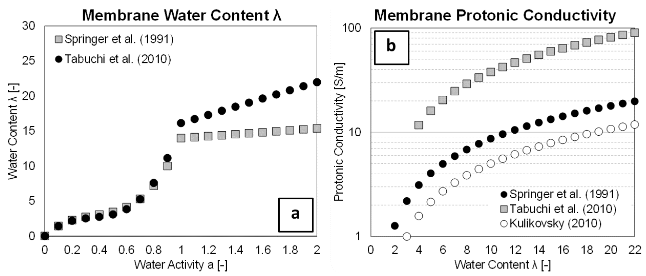
3.4.2. Membrane Water Content

The membrane hydration state is represented by the number of H₂O molecules per SO₃⁻ group, named water content $\lambda$, and equal to approximately 20 for fully-hydrated Nafion membranes. This is related to the water concentration in the membrane ionomer ($c_{H_{2}O}$, [$\mathrm{kmol}/{\mathrm{m}}^3$]), the membrane density (${\rho }_{m,dry}$, [$\mathrm{k}\mathrm{g}/{\mathrm{m}}^3$]) and the equivalent weight ($EW$, [$\mathrm{k}\mathrm{g}/\mathrm{kmol}$]) as in Equation (17). The membrane water content at equilibrium is usually related to the local water activity via algebraic expression, for which examples are reported in

Table 9. Correlations for membrane equilibrium water content $\lambda$.

Ref.	Correlation	Notes
[6]	$\lambda =\left\{\begin{array}{cc}0.043+17.81a-39.85a^2+36.0a^3,\hfill & \mathrm{for} 0<a<1\hfill \\ 14+1.4(a-1),\hfill & \mathrm{for} 1\le a\le 3\hfill \end{array}\right.$
[78]	$\lambda =\left\{\begin{array}{c}0.3+6a\left[1-\tanh (a-0.5)\right]+\hfill \\ +3.9\sqrt{a}\left[1+\tanh \left(\frac{a-0.89}{0.23}\right)\right]+s\left({\lambda }_{s=1}-{\lambda }_{a=1}\right),\hfill & \mathrm{for} s\le 0\hfill \\ 16.8s+{\lambda }_{a=1}(1-s),\hfill & \mathrm{for} s>0\hfill \end{array}\right.$	${\lambda }_{s=1}=16.8$ is the water content at saturation and ${\lambda }_{a=1}$ is the value obtained when $s=1$ and $a=1$.
[36]	$\lambda =\left\{\begin{array}{cc}0.03+18.43a-46.67a^2+44.36a^3,\hfill & \mathrm{for} 0<a<1\hfill \\ 16.15+5.85(a-1),\hfill & \mathrm{for} 1\le a\le 3\hfill \end{array}\right.$

and illustrated in Figure 4, showing that a good agreement is found for under-saturated states ($a<1$), whereas different values are reported for over-saturated conditions ($a>1$). The membrane water content is experimentally determined as a function of the local relative humidity and of water activity a as in Equation (18), where $p_{H_{2}O}$ represents the partial pressure of the water vapour. The relationship between the water concentration and water content $\lambda$ is given by Equation (17), with ${\rho }_{m,dry}$ the dry membrane density and $E{W}_m$ the membrane equivalent weight (represented by the dry mass of the membrane (ionomer) over the number of moles of SO₃⁻) which takes a value of 1100 $\mathrm{k}\mathrm{g}$/$\mathrm{k}$$\mathrm{mol}$ (for Nafion 112, 115 and 117) or 2100 $\mathrm{k}\mathrm{g}$/$\mathrm{k}$$\mathrm{mol}$ (for Nafion 211 and 212) [5].

$$\lambda =\frac{EW}{{\rho }_{m,dry}}{c}_{H_{2}O}$$

(17)

$$a=\frac{p_{H_{2}O}}{p_{sat,H_{2}O}}=\frac{x_{H_{2}O}·p_{abs}}{p_{sat,H_{2}O}}$$

(18)

As it will be shown in the following, the membrane water content $\lambda$ is a key property on which both the dissolved water flux and the protonic conductivity will be dependent, thus determining the rate of both species transport of interest.

3.4.3. Proton Transport in Membrane

For proton transport, a uniform H⁺ concentration in the membrane is assumed, thus also the second term in Equation (15) is null. Therefore, the H⁺ flux (i.e., the volumetric current density, $j_e$) reduces to a potential-gradient Ohm’s law (Equation (19)). Note that (Equation (19)) only describes the H⁺ flux in the membrane, while the source term for the charged species are included in Table 2.

$$j_e=-{\sigma }^{eff}\nabla {\Phi }_e$$

(19)

The membrane polymeric structure differs from the fibre-oriented one seen for GDL, and an isotropic approach for the charged species conductivity ${\sigma }^{eff}$ is more justified in this context. The effective ${\sigma }^{eff}$ depends on the membrane hydration state, thus it is a function of the water content $\lambda$. This is motivated by the different mechanisms of H⁺ migration in the membrane for increasing water content [5], moving from (I) direct-only H⁺ transfer between charged sites (for $\lambda <2$) to (II) water induced transport of H⁺ via H₃O⁺ ions (vehicular diffusion, similar to the the H⁺-induced electro-osmotic drag and relevant for $2<\lambda <13$) and (III) H⁺ migration between adjacent water molecules, as the polymer side chains are occupied by water molecules (hopping mechanism, dominating for $\lambda >13$)

Even if the mentioned mechanisms are not directly modelled in macro-homogeneous 3D-CFD models, their effect is synthesised by the Nafion protonic conductivity ${\sigma }^{eff}$ related to the water content $\lambda$. Correlations for ${\sigma }^{eff}$ for CFD models are reported in

Table 10. Correlations for membrane protonic conductivity ${\sigma }^{eff}$ in [$\mathrm{S}/\mathrm{m}$].

Ref.	Correlation	Notes
[6]	${\sigma }^{eff}=(0.5139\lambda -0.326)e^{1268\left(\frac{1}{303}-\frac{1}{T}\right)}$
[36]	${\sigma }^{eff}=(1.72\lambda -2.26)e^{2000\left(\frac{1}{303.15}-\frac{1}{T}\right)}$
[79]	${\sigma }^{eff}=0.5738\lambda -0.7192$

and illustrated in Figure 4, where an order of magnitude difference in the predicted ${\sigma }^{eff}$ is observed, indicating it as another relevant cause for modelling uncertainty.

3.4.4. Water Transport in Membrane

For water transport, also the first term in Equation (15) is null as water has no electron transfer in this context ($z_i=0$). Therefore, Equation (15) reduces to a Fickian-type transport flux towards negative gradient concentration (i.e., typically from cathode to anode). However, a secondary effect not included in the solute-independence hypothesis of the solution theory must be considered: the H⁺ migration to the cathode drags a number of H₂O molecules, opposing to the gradient-oriented transport. This effect is named electro-osmotic drag, and it is quantified by the electro-osmotic drag coefficient $n_d$ representing the number of transported moles of H₂O for each mole of H⁺. Several formulations from literature for $n_d$ are reported in

Table 11. Correlations for the electro-osmotic drag coefficient $n_d$.

Reference	Correlation
[6]	$n_d=\frac{2.5\lambda }{22}$
[80]	$n_d=\left[\frac{1}{{\left(0.35\lambda \right)}^4}+\frac{1}{1.{47}^4}\right]$
[81]	$n_d=0.0028\lambda +0.05\lambda -3.5·{10}^{-19}$
[82]	$n_d=\left\{\begin{array}{cc}1.0,\hfill & \mathrm{if} \lambda \le 14\hfill \\ \frac{1.5}{8}\left(\lambda -14\right)+1.0,\hfill & \mathrm{if} \lambda >14\hfill \end{array}\right.$

and illustrated in Figure 5. Note that all correlations generally predict an increase in $n_d$ for increased water content $\lambda$ (correlated with the water concentration), although their disagreement frames a still relevant uncertainty on this effect.

Another relevant influence of the membrane hydration state on its concurring transport mechanisms is the variation of the diffusion coefficient for the dissolved water, $D_{w,m}$. Several correlations from the literature are reported in

Table 12. Correlations for dissolved water diffusion coefficient $D_w$ in [${\mathrm{m}}^2/\mathrm{s}$].

Ref.	Correlation	Notes
[6]	$D_{w,m}={10}^{-10}{\mathrm{e}}^{2416\left(\frac{1}{303}-\frac{1}{T}\right)}\left(2.563-0.33\lambda +0.0264{\lambda }^2-0.000671{\lambda }^3\right)$
[83]	$D_{w,m}=\left\{\begin{array}{cc}3.1\times {10}^{-3}\lambda \left({\mathrm{e}}^{0.28\lambda }-1\right)·{\mathrm{e}}^{\left(\frac{-2436}{T}\right)},\hfill & \mathrm{for} 0<\lambda <3\hfill \\ 4.17\times {10}^{-4}\lambda \left(161·{\mathrm{e}}^{-\lambda }+1\right)·{\mathrm{e}}^{\left(\frac{-2436}{T}\right)},\hfill & \mathrm{for} 3\le \lambda <17\hfill \end{array}\right.$
[84]	$D_{w,m}=\left\{\begin{array}{c}\left(0.0049+2.02a-4.53a^2+4.09a^3\right)\hfill \\ D_0·{\mathrm{e}}^{2416\left(\frac{1}{303}-\frac{1}{T}\right)},\hfill & \mathrm{for} a\le 1\hfill \\ \left[1.59+0.159(a-1)\right]D_0·{\mathrm{e}}^{2416\left(\frac{1}{303}-\frac{1}{T}\right)},\hfill & \mathrm{for} a>1\hfill \end{array}\right.$	with $D_0=5.5\mathrm{e}-7\mathrm{c}\mathrm{m}/\mathrm{s}$
[81]	$D_{w,m}=\left\{\begin{array}{cc}{10}^{-10}{\mathrm{e}}^{2416\left(\frac{1}{303}-\frac{1}{T}\right)},\hfill & \mathrm{for} \lambda <2\hfill \\ {10}^{-10}\left[1+2(\lambda -2)\right]{\mathrm{e}}^{2416\left(\frac{1}{303}-\frac{1}{T}\right)},\hfill & \mathrm{for} 2\le \lambda <3\hfill \\ {10}^{-10}\left[3-1.67(\lambda -3)\right]{\mathrm{e}}^{2416\left(\frac{1}{303}-\frac{1}{T}\right)},\hfill & \mathrm{for} 3\le \lambda <4.5\hfill \\ 1.25·{10}^{-10}{\mathrm{e}}^{2416\left(\frac{1}{303}-\frac{1}{T}\right)},\hfill & \mathrm{for} \lambda \ge 4.5\hfill \end{array}\right.$
[26,85]	$D_{w,m}=4.1·{10}^{-10}{\left(\frac{\lambda }{25}\right)}^{0.15}\left[1+\tanh \left(\frac{\lambda -2.5}{14}\right)\right]$

for the implementation of $D_{w,m}$ in multidimensional CFD codes.

Finally, waster transport in the membrane is represented by an “extended Fickian” transport equation (Equation (20)), including both counteracting mechanisms. As for Equation (19), only the water flux in the membrane is included here, and source terms in Table 2, Table 3 and Table 4 are treated in Section 3.5.

$$J_{w,m}=-D_{w,m}\nabla c_{w,m}+\frac{n_{d}j}{F}$$

(20)

A final note is needed to underline that other water diffusion mechanisms are potentially present. One is the hydraulic permeation of membrane, related to possibly different pressure levels in the anode/cathode channels and superimposing to the ever-present water diffusion and electro-osmotic drag effects. Examples of its inclusion are models such as the Berning et al. [33] model, where a Schlögl equation (Equation (21)) is used for the liquid velocity ${\overrightarrow{u}}_l$, assuming a constant charge number ($z_f$) and concentration ($c_f$), and explicitly stating in the last term the hydraulic permeation effect.

$${\overrightarrow{u}}_l=\frac{k_{\Phi }}{{\mu }_l}{z}_f{c}_{f}F·\nabla \Phi -\frac{k_p}{{\mu }_l}·\nabla p$$

(21)

However, the pressure imbalance is in the order of ∼1–3 bar, and the very low permeability of Nafion allows to safely neglect this effect. For the same reason, the cross-diffusion of reactants from anode/cathode through the membrane is usually neglected.

3.5. Catalyst Layers: Key Modelling Aspects

Electrochemical reactions in a PEMFC develop within the Catalyst Layers (CL) or, more in detail, on the surface of the catalyst particles dispersed within this component. Two catalyst layers are present in a cell unit, an anodic (ACL) and a cathodic (CCL) one, and they are interposed between the membrane and the respective GDL. They constitute the electrochemical heart of the cell as it is where the half-reactions develop (see Equations (1) and (2)), representing the starting/ending site of charge species transport. The reaction kinetics and transport rates are strongly affected by the structure and composition of this component, for which modelling methods and accompanying assumptions might largely affect results. From a modelling standpoint, most of the effort is focused on CCL, where O₂, e⁻ and H⁺ ions combine to produce H₂O.

3.5.1. Modelling Approaches for CL

Several approaches to CL modelling can be found in the literature:

• Ultra-thin layer model: It is the simplest approach, consisting of neglecting the CL thickness and representing it with an infinitely thin surface where reactions take place as interfacial processes at the contact between membrane and GDL. Clearly, this approach is computationally very efficient and consequently attractive for the simulation of an entire cell. On the other hand, it prevents the analysis of the phenomena occurring within the catalyst layer and the role of the microstructure on cell performance. Berning and Djilali [86] used this model to analyse the effects of different parameters (e.g., GDL porosity and thickness) on the cell performance. However, note that this way to model the CL lead to an overestimation of the current density.
• Macro-homogeneous model (also called pseudo-homogeneous model): Similar to the GDL macro-homogeneous approach previously presented, it is a more accurate approach for CL modelling as it considers the finite CL thickness, with averaged transport coefficients describing the effect of variations in compositional parameters describing platinum catalyst, carbon support, solid GDL matrix and electrolyte materials [87]. However, it cannot assess the complex multi-material structure of the CL.
• Agglomerate model: It is the most complex and sophisticated approach, including both the composition and the structural distribution of CL materials. Generally, in this type of approach the CL is composed by agglomerates, each of them presenting ionomer and Pt/C particles. Agglomerate models results agree with experimental observations showing that a CL is composed by the agglomeration of catalyst particles (Pt and C) and an ionomer [88]. There are two types of pores, primary and secondary: the former are the internal pores within the agglomerates, while the latter are between the different agglomerates. The primary pores inside the agglomerate could be filled by an ionomer phase, as in the model presented in [88]. In this case, within these pores the diffusion of the reactants is permitted only in the dissolved phase, whereas the secondary pores may be partially or fully filled with liquid water. Each agglomerate has a radius and may be covered with an ionomer film of uniform thickness. Another agglomerate model is the one presented by Xing [89], where the generated liquid water occupies the void spaces of both the primary and secondary pores, reducing the void space. The generated liquid water is initially formed inside the primary pores, partially occupying the space until it fills them completely. When the primary pores are fully filled, the liquid water fills the secondary pores as a thin film surrounding the carbon agglomerate. This means that the presence of liquid water in the secondary pores depends on the filling of the primary pores. The effective species diffusivity in the primary pores will therefore be composed of the diffusivity through (I) the ionomer phase, (II) the liquid phase and (III) the void space, whereas the effective species diffusivity in the secondary pores will depend on the volume fraction of liquid.

3.5.2. Electrochemistry Modelling in CL

Catalyst layers require a dedicated treatment as they host the electrochemical reactions. From the point of view of species creation/destruction, this is handled by the species transport equation (see Table 1, Table 2 and Table 3) via the source term $S_i$ (Table 2, Table 3 and Table 4). This is normally expressed for a H₂/air PEMFC as in Equation (22), where the terms $S_{H_2,a}$, $S_{O_2,c}$ and $S_{H_{2}O,c}$, consider the consumption/production of H₂, H₂ and H₂O, respectively.

$$\begin{array}{ccc}\hfill S_{H_2,a}& =-\left(\frac{M_{H_2}}{2F}\right)j_a;S_{H_{2}O,a}=-M_{H_{2}O}\left(\frac{n_d{j}_a}{F}\right),\hfill & \hfill \mathrm{in}\mathrm{ACL}\\ \hfill S_{O_2,c}& =-\left(\frac{M_{O_2}}{4F}\right)j_c;S_{H_{2}O,c}=M_{H_{2}O}\left(\frac{n_d{j}_c}{F}\right)+\left(\frac{M_{H_{2}O}}{2F}\right),\hfill & \hfill \mathrm{in}\mathrm{CCL}\end{array}$$

(22)

This bundled expression for $S_i$ is particularly suited for the single-phase/MMP method, while it is not formally appropriate to the EMP approach as the water phase is not made explicit in Equation (22). The $S_{H_{2}O}$ terms also include the water flux from anode to cathode accompanying proton migration, i.e., the electro-osmotic drag effect discussed in Section 3.4.

As discussed in Section 3.1, the diffusion coefficients for the i-th species ($D_i^{eff}$) are related to the porosity of the media using the Bruggeman correlation as in Equations (6)–(9). Considering the blockage of liquid water and the reduced size of CL pores, it can be assumed that liquid water has the similar effect as the solid materials. Therefore, Equation (7) can be modified in Equation (23) including the liquid water volume fraction s [5]:

$$D_{i,0}^{\ast }=D_{i,0}·{ϵ}^{1.5}·{(1-s)}^{1.5}$$

(23)

The charge conservation equations for solid and electrolyte phases are obtained by applying the Ohmic’s Law as in Table 1 and Table 2, where ${\sigma }^{eff}$ and ${\kappa }^{eff}$ are the effective ionic and electrical conductivity in ionomer and solid phase, respectively, and ${\Phi }_e$ and ${\Phi }_s$ are the ionomer and electrical phase potentials, respectively. In the charge equations in Table 1, the source terms ($S_{\Phi ,s}$, $S_{\Phi ,e}$) are only present in the CL, and they express the volumetric transfer current (charge flux). The $j_a$ and $j_c$ terms are given by the Butler–Volmer Equation (24):

$$\begin{array}{ccc}\hfill j_a& ={\zeta }_a·j_{0,a}^{ref}·{\left(\frac{c_{H_2}}{c_{H_2}^{ref}}\right)}^{{\gamma }_a}·\left[{\mathrm{e}}^{\left(\frac{{\alpha }_{a}F{\eta }_a}{RT}\right)}-{\mathrm{e}}^{\left(\frac{-{\alpha }_{c}F{\eta }_a}{RT}\right)}\right],\hfill & \hfill \mathrm{in}\mathrm{ACL}\\ \hfill j_c& ={\zeta }_c·j_{0,c}^{ref}·{\left(\frac{c_{O_2}}{c_{O_2}^{ref}}\right)}^{{\gamma }_c}·\left[-{\mathrm{e}}^{\left(\frac{{\alpha }_{a}F{\eta }_c}{RT}\right)}+{\mathrm{e}}^{\left(\frac{-{\alpha }_{c}F{\eta }_c}{RT}\right)}\right],\hfill & \hfill \mathrm{in}\mathrm{CCL}\end{array}$$

(24)

Normally, ${\gamma }_a$ and ${\gamma }_c$ are pressure scaling coefficients equal to 0.5 and 1, respectively, and $c_{H_2}$, $c_{H_2}^{ref}$, $c_{O_2}$ and $c_{O_2}^{ref}$ are the hydrogen and oxygen local and reference concentrations. The specific active surface area of the catalyst (${\zeta }_a$ and ${\zeta }_c$, [$1/\mathrm{m}$]) is related to the catalyst surface area per unit mass of the catalyst ($A_s$, [${\mathrm{m}}^2/{\mathrm{g}}_{\mathrm{Pt}}$]), the Pt loading ($m_{Pt}$, [${\mathrm{g}}_{\mathrm{Pt}}/{\mathrm{m}}^2$]) and the thickness of the catalyst layer (${\delta }_{CL}$, [$\mathrm{m}$]) [90] as in Equation (25):

$$\begin{array}{ccc}\hfill {\zeta }_a& =\frac{A_s^a{m}_{Pt}^a}{{\delta }_{CL}^a},\hfill & \hfill \mathrm{in} ACL\\ \hfill {\zeta }_c& =\frac{A_s^c{m}_{Pt}^c}{{\delta }_{CL}^c},\hfill & \hfill \mathrm{in} CCL\end{array}$$

(25)

Typical Pt loading is between 2–4 ${\mathrm{g}}_{\mathrm{Pt}}$/${\mathrm{m}}^2$, although different values between ACL and CCL are often applied albeit they are rarely indicated. In such cases, CCL is preferred for Pt loading with the aim to reduce its activation overpotential.

The catalyst-specific surface area $A_s$ strongly depends on different types of supported catalysts and platinum black. Nevertheless, it may be approximated in terms of the platinum mass fraction f (in this case $A_s$ [${\mathrm{m}}^2/{\mathrm{g}}_{\mathrm{Pt}}$]) as in Equation (26):

$$A_s=(227.79f^3-158.57f^2-201.53f+159.5)\times {10}^3$$

(26)

In

Table 13. Exchange current density and transfer coefficients from literature. The table continues in the bottom part for additional references and variables.

Ref.	$j_{0,a}^{ref}[\mathbf{A}/{\mathrm{m}}^2]$	$j_{0,c}^{ref}[\mathbf{A}/{\mathrm{m}}^2]$	${\alpha }_a$	${\alpha }_c$
[77]	$1.0\times {10}^4$	1	$0.5$	$0.8$
[90]	$3.0\times {10}^3$	$0.3$	$1.0$	$0.8$
[91]	$3.5$	$3.5\times {10}^{-4}·\exp \left[\frac{-7900·(353.15-T)}{353.15·T}\right]$	$0.5$	$0.5$
[87]	−	${10}^{0.037·T-16.96}$	$0.5$	$1.0$
[92]	$3.5·\exp \left[\frac{-1400(353.15-T)}{353.15·T}\right]$	$3.5\times {10}^{-4}·\exp \left[\frac{-1400(353.15-T)}{353.15·T}\right]$	$0.5$	$0.5$
[93]	$1.0\times {10}^4$	$\left[{10}^{\left(3.507-\frac{4001}{T}\right)}\right]\times {10}^4$	1	$0.495+2.3\times {10}^{-3}(T-300)$
Ref.	$j_{0,a}^{ref}·{\zeta }_a$ [$\mathrm{A}/{\mathrm{m}}^3$]	$j_{0,c}^{ref}·{\zeta }_c$ [$\mathrm{A}/{\mathrm{m}}^3$]	${\alpha }_a$	${\alpha }_c$
[28]	$1.0\times {10}^{-9}$	$3.0\times {10}^5·\exp \left[0.014189(T-353)\right]$	$1.0$	$1.0$

, several values from the literature for the reference exchange current densities $j_{0,a}^{ref}$ and $j_{0,c}^{ref}$ are reported. Moreover, in some cases it is indicated directly that $j_{0,a}^{ref}·{\zeta }_a$ and $j_{0,c}^{ref}·{\zeta }_c$, whereas ${\alpha }_a$ and ${\alpha }_c$ are the transfer coefficients.

A widely adopted correlation relating $j_{0,c}^{ref}$ (here in $\mathrm{A}/{\mathrm{cm}}^2$) and T is obtained from a curve fit of experimental data presented in [94] (Equation (27)):

$$lo{g}_{10}\left(j_{0,c}^{ref}\right)=3.507-\frac{4001}{T}$$

(27)

In the majority of the numerical studies, the resulting polarisation curve from simulations is compared to the experimental one. Unfortunately, the phase interaction area and reference exchange currents density are commonly adjusted to fit the numerically predicted curve to its corresponding experimental values, introducing an undesired model tuning which could easily hide modelling inaccuracies. Regarding the anodic transfer coefficient ${\alpha }_a$, the Pt electrode seems to be independent of temperature for HOR and ${\alpha }_a=0.5$ is widely reported. The situation is different at cathode, where usually two Tafel slopes are obtained for ORR: a low (≃ 60 $\mathrm{m}$$\mathrm{V}$/dec) and a high slope (≃ 120 $\mathrm{m}$$\mathrm{V}$/dec), depending on the potential range and electrode materials used [95]. The high slope regime is typically that one when the cell potential is below $0.8$ $\mathrm{V}$. Note that the cathodic transfer coefficient (${\alpha }_c$) is unity for the low slope regime, while in the high slope regime it varies with temperature according to Equation (28) [96]. Another expression for the dependence of ${\alpha }_c$ on temperature is Equation (29) [97]:

$${\alpha }_c=0.495+2.3·{10}^{-3}·(T-300)$$

(28)

$${\alpha }_c=\left(0.001678\right)T$$

(29)

A recent study showed that in high-temperature PEMFCs ( 120 ${}^{\circ }\mathrm{C}$), the relative humidity of the cathodic stream ($R{H}_c$) dependence of ${\alpha }_c$ follows Equation (30):

$${\alpha }_c=(0.001552·R{H}_c+0.000139)T$$

(30)

3.5.3. Dissolved Water Treatment in CL

The simplified treatment of the water source terms $S_{H_{2}O}$ in the previous section suffers from the inability to distinguish between the three phases of water existence, i.e., vapour, liquid and dissolved. An improved description of $S_{H_{2}O}$ is advisable because (I) all three phases coexist in CL, (II) water is formed in dissolved phase [26] and (III) it is formally required if the EMP method is used for multi-phase fluid treatment. The dissolved water steady-state transport in membrane/CL is described by Equation (31), where the dissolved water flux $J_{w,m}$ is from Equation (20) and $S_d$ is the dissolved water source term. This last is expressed as in Equation (32):

$$\nabla J_{w,m}+S_d=0$$

(31)

$$S_d=\left\{\begin{array}{cc}{S}_{gd}+S_{ld},\hfill & \mathrm{in} \mathrm{ACL}\hfill \\ S_{gd}+S_{ld}+S_{\lambda }\hfill & \mathrm{in} \mathrm{CCL}\hfill \end{array}\right.$$

(32)

The terms composing $S_d$ describe the separate water transition from gas to dissolved ($S_{gd}$) and from liquid to dissolved ($S_{ld}$) due to sorption reactions, and in dissolved phase ($S_{\lambda }$, only present at CCL) due to electrochemical reactions. A detailed description of these terms is given in [26], and their relevance cannot be neglected for non-equilibrium conditions.

3.5.4. Heat Generation in CL

Alongside the heat generation due to the Joule effect present in all the conductive parts (BPP, GDL and membrane), CL hosts an additional heat generation contribution associated to the irreversible reactions developing herein. The energy transport equation in steady-state conditions is presented in Table 1 and Table 3. The source term $S_T$ in the single-phase/MMP approach can be expressed as in Equation (33), whereas in the EMP method it can be more precisely described as in Equation (34), including the thermal contributions of water phase transition and absorption using the latent heat of condensation ($h_w$) and of absorption/desorption ($h_{w,m}$) [77]:

$$S_T=j\left[\eta +T\frac{\Delta S}{nF}\right]+\frac{i_s^2}{{\sigma }^{eff}}+\frac{i_e^2}{k^{eff}}$$

(33)

$$S_T=\left\{\begin{array}{cc}{j}_a\left[{\eta }_a+T\frac{\Delta S_a}{nF}\right]+\frac{i_s^2}{{\sigma }^{eff}}+\frac{i_e^2}{k^{eff}}+S_{gl}{h}_w+S_{gd}{h}_{w,m},\hfill & \mathrm{in} \mathrm{ACL}\hfill \\ j_a\left[{\eta }_c+T\frac{\Delta S_c}{nF}\right]+\frac{i_s^2}{{\sigma }^{eff}}+\frac{i_e^2}{k^{eff}}+S_{gl}{h}_w+S_{ld}(h_{w,m}-h_w),\hfill & \mathrm{in} \mathrm{CCL}\hfill \end{array}\right.$$

(34)

4. Validation Techniques for CFD Simulation of PEM Fuel Cells

As mentioned in Section 3, the modelling of PEM fuel cells involves a considerable number of (material) parameters. Many of these parameters are unknown and must be obtained by measurements or by literature research. In addition, the developed models for PEM fuel cells need to be validated. Therefore, the first part of the next section, Section 4.1, focuses on the whole stack’s measurement techniques to receive input and output values, i.e., species mass flows and fractions, electrical current/voltage and temperature distributions. The second part, Section 4.2, focuses on the measurement techniques of material parameters of the cell parts, i.e., electrical/protonic conductivities, water diffusion/electro-osmotic drag coefficients and permeability/porosity.

4.1. Measurement Techniques for Fuel Cell Stacks

Besides the standard measurement values (electric current, voltage, humidity, mass flow, pressure and temperature) at predefined locations, the more advanced methods, which provide a more detailed analysis, will be outlined in the next section.

For the in-depth analysis of fuel cells, numerous advanced measurement methods exist. The methods include the determination of operating parameters on fuel cell performance (in situ characterisation, i.e., during operation) and material properties (ex situ characterisation of the individual components composing the fuel cell). Furthermore, electrochemical techniques (electrochemical impedance spectroscopy, cyclic voltammetry, etc.) represent a powerful diagnostic tool set, but these techniques solely measure the average property of the whole electrode. For the validation of numerical models, the local effects and properties are of interest. In the following sections, the applicable in situ measurement methods to validate the CFD results of an operating fuel cell are presented: gas composition of the anode and cathode, liquid water content, current density distribution and temperature distribution [98,99,100,101,102,103].

4.1.1. Gas Composition Anode/Cathode

For the determination of the gas composition of the cathode/anode and the contained particles therein, the following methods are presented in the literature.

Infrared Spectroscopy

Infrared spectroscopy determines the absorption of light in the infrared region of the electromagnetic spectrum for different gaseous components. It was used by Miyaoka et al. [104] for the measurement of the NH${}_3$ content in hydrogen (NH${}_3$ was used as a hydrogen carrier to store energy). Furthermore, Maass et al. [105] utilised this method to measure the concentrations of CO${}_2$ and CO in the range of ppm at the cathode outlet (in nitrogen and oxygen atmosphere) during fuel cell operation. Infrared spectroscopy is also often applied in conjunction with the mathematical process of a Fourier-transform (Fourier-transform infrared spectroscopy (FTIR)), which allows for investigations with wider spectral ranges.

Mass Spectrometer

When atoms and molecules are ionised (electrically charged), they can be deflected by magnetic fields. This phenomenon is used by mass spectrometry. Depending on the mass of the ionised particle, the deviation differs and the mass of the particle can be determined. As a result, Lim et al. [106] applied this method to measure the content of O${}_2$ and CO${}_2$ in the anode exhaust gas. Furthermore, Shao et al. [107] utilised online mass spectroscopy to detect particles in the gas flow under fuel starvation (which is associated with aging effects).

Gas Chromatography

A gas chromatograph uses a carrier gas (usually nitrogen or helium) in which the gas sample is injected. A detector determines the molecules in the gas. There are different types of detectors depending on the application, e.g., detectors that respond to specific types of molecules or carbon–hydrogen bonds. Liu et al. [108] analysed gas samples of the anode to determine the nitrogen concentration under different load conditions. As a result, the nitrogen crossover coefficient was obtained. David et al. [109] mentioned that gas chromatography was used by various other authors to determine the water vapour inside the cell.

Colorimetric Tubes

A fast and easy-to-use method to detect specific gas concentrations in a sample are colorimetric tubes. The sample is injected into a tube which contains a reagent. The resulting colour change is proportional to the concentration of the substance being investigated. The concept is similar to pH paper, which is used to determine acids and bases. Miyaoka et al. [104] roughly estimated the NH${}_3$ concentration with a measuring range of 0.2ppm–20ppm.

4.1.2. Liquid Water Content

The water content inside a fuel cell is a crucial factor for the proper operation. If liquid water blocks the gas feed to the catalyst, no reaction can take place and the power of the cell is reduced. Likewise, if the water vapour content is too low and the humidification of the membrane is insufficient, proper proton conduction is not guaranteed and increased ohmic losses are the consequence. Therefore, the proper water and humidity management inside the cell is of utmost importance. Various in situ methods have been developed to investigate liquid water inside the cell, such as the transparent cell, which offers a comparably easy and fast way to optically visualise water after some initial design changes of the cell (optical access of the flow field). Other methods, such as neutron imaging, X-ray imaging and magnetic resonance imaging, show increased complexity and limitations to spatial and temporal resolution, but allow for investigation with less deviation from the original cell design [110,111].

Transparent Cell

For the optical assessment of the flow channels (by means of a optical camera), the opaque bipolar plates (usually metal or carbon is used) have to be redesigned. A certain part of the bipolar plate (usually around 1 mm thickness) is replaced by polycarbonate, which offers the advantage of high light transmittance. Replacing the original bipolar plate material may affect the in situ investigation, but the comparably easy optical access represents a clear advantage [112]. By utilising this method, the liquid water inside the flow channels (anode and cathode side) can be optically visualised [113].

Neutron Imaging

The method of neutron imaging is based on the attenuation of neutrons, which shows certain similarities to X-ray imaging. However, the neutron attenuation is not related to the density of the material (as it is for X-rays), but only the neutron attenuation property of the material itself, so that images through metal plates are possible. Depending of the direction of the neutron beam through the cell, different aspects can be investigated: if the beam is parallel to the membrane plane, the water content of the anode or cathode can be visualised. If the neutron beam is perpendicular to the membrane plane, it enables the investigation across the lateral extend of the cell [114]. Neutron imaging offers the advantage of high contrast in situ water distribution investigations with excellent penetration through typical bipolar materials, such as aluminium, graphite or steel. This method has been applied for almost two decades to asses the effects of different flow channels geometries and operating conditions [115,116]. The measured water thickness accuracy is stated to be in the range of 5–10 $\mathsf{\mu }\mathrm{m}$ [117].

X-ray Imaging

X-ray imaging is based on the additional attenuation of photons (depending on the density of material) when liquid water is present in fuel cells. It offers high spatial resolution (below 10 $\mathsf{\mu }\mathrm{m}$) and high temporal resolution (less than 10 $\mathrm{s}$), which is sufficient to analyse the dynamic liquid transport behaviour of fuel cells [118]. The sample is placed between the X-ray source and a detector, which is used to visualise the attenuation of the beam. Utilising this technique, the opaque materials of a cell do not prevent the in situ liquid water formation and transport investigation in the channels and gas diffusion layers [119]. Moreover, it offers the possibility to analyse the cell from the side (in contrast to optical investigations of transparent cells perpendicular to the membrane), which is critical to capture droplet formation and droplet height [120]. Banerjee et al. [121] reported X-ray images of $6.5$ $\mathsf{\mu }\mathrm{m}$/pixel and 0.33 frames per second, which were deemed sufficient to capture changes in membrane hydration.

Magnetic Resonance Imaging

For this method, a strong magnetic field and radio waves (which resonate with specific atoms) are used. The radio waves interact with the magnetic properties of the sample. Receiver coils around the sample receive the signal. Magnetic resonance imaging is used to examine water motion within the membrane and flow fields. For the investigation, the materials of the cell must be compatible with strong magnetic fields, thus ferromagnetic materials (iron, nickel and cobalt) must be avoided [122]. A disadvantage of this method is the limited spatial ( 25 $\mathsf{\mu }\mathrm{m}$) and temporal resolution [111,123]. Tsushima et al. [124] stated that the strong magnetic field has no significant effect on the cell performance, so that the investigation is not disturbed by the specific method.

Raman Spectroscopy

This method uses a laser as a source to analyse the backscattered light spectra at different depths along the membrane thickness [125]. The laser source and the recorder are typically attached to the bipolar plate through a cylindrical access [126,127]. Depending on the recorded spectra, the sorbed water/state of hydration of the membrane during operation can be determined at a specific point of the membrane.

4.1.3. Current Density Distribution

For the assessment of the current density, typically special probe preparation is required (preparation or modification of cell components). The methods are printed circuit boards and segmented cells. Besides, magnetic resonance can be applied, which is a noninvasive method [128].

Printed Circuit Board (PCB)

For this method, an array of shunt resistors on a printed circuit board (PCB) is used to measure the current. Depending on the segmentation of the cell and the number of shunt resistors, the spatial resolution of the distribution can be adjusted. Rasha et al. [129] applied an 14 × 14 array of shunt resistors across a 100 ${\mathrm{cm}}^2$ cell. Furthermore, Peng et al. [130] utilised 144 current collecting segments and shunt resistors for a 250 ${\mathrm{cm}}^2$ and 3 $\mathrm{k}$$\mathrm{W}$ level fuel cell stack.

Segmented Cells

The segmented cells method is similar to the printed circuit boards method. The current of each segment of a cell is measured. Reshetenko and Kulikovsky [131] used 10 segments with an area of $7.6$ ${\mathrm{cm}}^2$ each; every segment has its own current collector and GDL. The segmentation was applied to the cathode, and the gas flow was directed consecutively through the 10 segments. Chevalier et al. [132] used 11 segments for a 12 ${\mathrm{cm}}^2$ cell. Shunt resistors or Hall-effect sensors can be used for the current measurement [133].

Magnetic Resonance

Magnetic resonance is based on a static external magnetic field in combination with rf (radiofrequency) coils that are applied to the fuel cell. When the fuel cell generates electric current, both the static magnetic field and the magnetic field generated by fuel cell current are detected by the coils. As a result, the electric current of the cell can be measured. This method allows noninvasive investigations on the current density of the cell. Typically, this method is used to detect the water content of the fuel cell. Yet, Ogawa et al. [134] utilised this method to determine the current distribution by an inverse analysis that reproduces the spatial distribution of the resonance frequency of the signals. Rf coils arranged in 7 rows and 7 columns were placed into the MEA. The frequency of the nuclear magnetic resonance signal, which is proportional to the magnetic field strength (and therefore the electric current), is received by the coils. The two-dimensional spatial distribution of the coil signals is used to determine the current density across the cell.

Magnetotomography

This method allows noninvasive investigations on the current density of the cell. It is based on the measurement of the magnetic flux surrounding a single fuel cell or a stack caused by the electric current. Hauer et al. [135] developed a four-axis positioning system with a 3-D magnetic flux sensor to visualise and investigate the current density distribution. Plait et al. [136] designed a new magnetic field analyser device with a ferromagnetic circuit for the magnetic flux sensors, which is essentially different to other devices using this principle. The authors state to have achieved a more accurate analysis of the current distribution utilising this type of sensors.

4.1.4. Temperature Distribution

For the proper humidity management, the temperature of the cell is crucial. Depending on the size of the cell, the temperature distribution can cause varied performance across the cell.

Infrared Thermography

This comparably easy method does not require any preparation of the fuel cell. An infrared camera can be used to measure the surface temperature of the cell under different operating conditions [137].

Micro-Thermocouples

This technique uses several thermocouples which are integrated into the bipolar plates. Wilkinson et al. [138] used this technique to measure the temperature at the interface of the gas diffusion layer and the graphite bipolar plate.

In-Fibre Bragg Grating (FBG) Sensors

This method is similar to micro-thermocouples, but in contrast to conventional thermocouples, optical fibres are used. The measurement principle is based on the reflection and transmission of particular wavelength in the fibre. The advantage is that fibres are comparably small, immune to moisture, provide minimal impact on cell performance and are unaffected by the electrochemically active environment [139].

4.2. Measurement Techniques for Material Parameters

The setup of a CFD simulation model requires a significant amount of material properties for the different parts, e.g., sulfonic acid group concentration, water diffusion and electro-osmotic drag coefficient for the membrane, the porosities and permeabilities for GDL and CL or electrochemical parameters of the CLs. Identifying the most critical material parameters with the biggest influence on the solution is based on the research of Karpenko-Jereb et al. [140]. Their findings agreed well with the authors’ own experience. In [140], a computational mesh with hexahedral cells of a straight, single-channel PEM-fuel cell was created. This mesh was further used to perform CFD simulations with varying material properties. The reference solution $x_0$ was followed by two simulations: one with 50% lower value ($x_0·0.5$) and the other with 50% higher value ($x_0·1.5$) of the corresponding material parameter. For the present paper, the material parameters were categorised by the deviation of the resulting current density according to

• high impact: current density deviates by more than 10% (absolute) or
• medium impact: current density deviates between 5% to 10% (absolute)

The bar graph in Figure 6 shows the influence of the material parameters on the simulated current density:

With the capital letters representing the following material parameters:

(A)

Membrane thickness

(B)

Membrane ionic conductivity

(C)

Cathode CL thickness

(D)

Cathode CL exchange current density

(E)

GDL thickness

(F)

GDL porosity

(G)

GDL electrical conductivity

(H)

Membrane sulfonic acid group concentration

(I)

Membrane water diffusion coefficient

(J)

Cathode CL transfer coefficient

(K)

GDL contact angle

Therefore, the classification in high and medium is as follows: (A–G) high impact and (H–K) medium impact. Al-Baghdadi and Al-Janabi [141] performed a parametric study on material properties, such as GDL thickness and porosity as well as membrane thickness. They came to a similar conclusion as [140]: that the membrane and GDL thickness significantly impact overall fuel cell performance.

According to this classification, the correct determination of the material parameters from the high-impact pool is crucial in order to achieve accurate simulation results of the fuel cell’s current density and voltage. Therefore, the focus of the present chapter will be on the determination of these parameters. However, the measurement methods for the material parameters from the medium-impact pool will be mentioned as well.

4.2.1. Thickness Measurement

Other authors confirmed the influence of the membrane thickness on the overall fuel cell performance [141,142]. The thickness of the membrane without electrodes can be measured using simple tools like a thickness gauge [143]. In contrast, the determination of catalyst layer thickness is a more challenging task. The catalyst layer is located between the membrane and the gas diffusion layer (GDL) and has a typical thickness of 5–20 $\mathsf{\mu }\mathrm{m}$ [144,145]. Membranes with two electrodes (anode and cathode) are called MEAs or Catalyst-Coated Membranes (CCMs) [146]. Catalyst layers consist of carbon particles with embedded platinum (Pt/C particles), and these particles are mixed with ionomer powder [147,148]. The mixture is hand-painted, air-brushed, sputtered or screen-printed onto the membrane. This approach ensures good bonding of the catalyst layer with the membrane and a high number of triple-phase boundaries (TPB) to achieve good overall performance of the fuel cell [149,150]. Keeping the manufacturing process in mind, the individual measurement of anode/cathode catalyst layer and the membrane is challenging. Destructive methods like scanning electron microscopy or scanning transmission X-ray microscopy [151,152,153,154,155,156] and non-destructive methods like 3D imaging with X-ray Computed Tomography (XCT) were developed to measure the thicknesses.

For scanning electron microscopy (SEM) or scanning transmission X-ray microscopy (STM), a proper preparation of the probe like cutting, handling and viewing under vacuum conditions has to be ensured. CCM probes for STM measurements need to be embedded into epoxy or polymers like polystyrene (PS) [155,156,157] to stabilise the probe. After embedding, fragile probes of about 100 $\mathrm{n}$$\mathrm{m}$ are cut from the samples and analysed. The whole process has to take place under vacuum and can cause unwanted dehydration of the ionomer. Furthermore, the sample could be damaged by charged particles (e.g., electrons) used by SEM or TEM. For investigations on the degradation of the MEA, the different layers cannot be distinguished any more due to the chemical and structural altering of the probe [147].

The XCT method helps to overcome the mentioned limitations and is a completely non-destructive method. White et al. [158] and Pokhrel et al. [147] investigated the carbon corrosion of the cathode catalyst layer (CCL) and the accompanying thickness reduction. The XCT method was further used to analyse parameters of different length scales. On the micron length scale, the thickness, uniformity and morphology of fuel cell electrodes during different manufacturing processes were visualised [149]. On the nano length scale, the pore structures of the catalyst layer were investigated [159]. Usually, a sample was mounted on a rotating table and hundreds of 2D slices were produced. These pictures were used to compute a 3D volume with the help of specialised software and computer clusters. The process can be repeated several times without damaging the probe itself. The active area of the samples ranging from approximately 9–36 ${\mathrm{mm}}^2$ [158,160,161]. With the XCT method, it is possible to perform 4D (the fourth dimension is time) in situ measurements to visualise the fuel cell’s degradation. Figure 7 shows XCT based cross-sectional views of the MEA at different degradation stages. The thickness can be determined with elaborated computer programs. More information on this topic can be found in [158,161].

4.2.2. Ionic Conductivity

The ionic conductivity of the polymer membrane (ionomer, electrolyte) greatly influences the overall fuel cell performance and voltage per current density [162]. The ionic conductivity strongly depends on the water content of the membrane [162,163]. Thus, a fuel cell system’s water management is crucial for high performance [164,165]. The water transport mechanisms within a polymer membrane are further discussed in Section 4.2.3. Despite other important (material) parameters, Karpenko-Jereb et al. [140], Lee et al. [162] and Figure 6 depicted the importance of conductivity investigations of membrane and GDLs for detailed numerical approaches like CFD-simulation.

The main methods to determine the ionic conductivity of membranes are alternating (AC) or direct current (DC) impedance measurements. These methods are based on the measurement of the probe’s resistivity during the application of electrical or ionic current. Electrochemical impedance spectroscopy (EIS) is not only used for ex situ measurements of material characterisation or single parts of the fuel cell, but can also be applied for in situ measurements of the fuel cell or whole stack [166,167,168]. Rezaei Niya and Hoorfar [167] reviewed the application of EIS for in situ measurements for PEM fuel cell systems.

The basic principles of EIS can be found in [98,162,165,166,167,169,170,171,172,173,174,175,176,177], but a short overview is given in the following. For EIS measurements, harmonic perturbations are applied to the probes, and the impedance response is recorded over a wide frequency range. The impedance Z is the ratio of the oscillating voltage $\tilde{U}$ and current density $\tilde{j}$ and is defined as a complex number. A negative sign is required to be consistent with the definition of a positive current [168].

$$Z=-\frac{\tilde{U}}{\tilde{j}}$$

(35)

The measurement of the impedance response for different frequencies requires a frequency response analyser (FRA). The FRA applies a sinusoidal current to the fuel cell or membrane through a load bank. The response of the system is captured and analysed by the FRA. After capturing the system response, an impedance spectrum is calculated [166,167]. For probes with low resistance, a four-electrode configuration, see Figure 8a, reduces the interfacial resistance and polarisation during measurement. Two electrodes are mainly used for samples with high resistance ($>10 \mathrm{k}\Omega$) because the resistivity of the lead itself is low enough to be neglected [162]. A Nyquist plot (rectangular form $Z^{\prime }+j{Z}^{″}$) or a Bode plot with the logarithm of the magnitude $\log \left(\right|Z\left|\right)$ vs. the logarithm of the frequency $\log \left(\omega \right)$ can be used to present the complex impedance [162]. A typical complex impedance spectrum (Nyquist plot) of a Nafion membrane is shown in Figure 9.

The equivalent circuit consists of ohmic resistances and capacitors, as the membrane also has a capacitive part. Therefore, the impedance is calculated via $Z=Z^{\prime }+j{Z}^{″}=\sqrt{R^2+{(X_L+X_C)}^2}$ with R ohmic resistance, $X_L$ inductive and $X_C$ capacitive reactance. With $\sigma =d/(R·A)$, where d is the length between the electrodes, A is the sample area and R the ohmic resistance from the Nyquist plot where the half-circle of the impedance crosses the real axis, the ionic conductivity of the membrane can be determined [162,167,178].

Beattie et al. [170] and Gardner and Anantaraman [172] conducted AC impedance measurement using the coaxial probe method, see Figure 8b. The open end of the coaxial probe element is pressed to one open end of the investigated membrane. This method’s main advantage is that the accessibility to the membrane needs to be ensured only from one side. In addition, environmental influences such as temperature and humidity can be controlled easily. For membranes thicknesses that are small compared to the probe’s gap size ($b-a$, Figure 8b), the current distribution is nearly uniform. Then, the ionic conductivity of the membrane can be obtained by a simple relationship [172]:

$$\sigma =\frac{1}{2\pi R_{T}h}ln\left(\frac{b}{a}\right)\mathrm{with}{R}_T=\frac{R_S}{2\pi }ln\left(\frac{b}{a}\right)$$

(36)

with membrane thickness h, measured resistance $R_T$ and surface resistivity $R_S=1/\left(\sigma h\right)$. If the thickness of the membrane is large compared to the gap size, a more complicated calculation is necessary. For more details, see Gardner and Anantaraman [172].

Karpenko et al. [173] investigated the difference, differential-difference and mercury-contact method for measuring the ionic conductivity.

Büchi and Scherer [179] researched the resistivity of the membrane as a function of current density with in situ measurements. They used current pulses to determine the resistivity of the membrane and concluded that there is a remarkable increase in resistivity for current densities >$0.5\mathrm{A}/{\mathrm{cm}}^2$.

Lee et al. [162] and others [163,180,181] investigated the dependence of the ionic conductivity on the temperature and water content as well. They showed that the temperature dependence can be modelled with an Arrhenius type formula [182,183].

4.2.3. Water Diffusion Coefficient/Electro-Osmotic Drag Coefficient

The water management of a PEM fuel cell is very important for high performance as the ionic conductivity strongly depends on the water content [164]. Water diffusion and electro-osmotic drag are two crucial water transport mechanisms within perfluorosulfonate acid (PFSA) membranes. Convection generated by pressure gradient is the third water transport mechanism [184]. Recent works also reported a fourth mechanism, thermo-osmosis, arising from temperature gradients [185]. However, the latter two are not discussed in this context.

The main methods to measure the diffusion coefficient of water in polymer membranes are the pulse field gradient spin echo nuclear magnetic resonance (PGSE-NMR) method [165,186,187,188,189], radioactivated-tracer techniques [190,191,192,193,194] and by the change of weight of the membrane on sorption/desorption of water from the vapour phase [195].

Superconducting magnets and spectrometers were used for PGSE-NMR measurements. The samples were stored at a constant temperature before the measurements to get equilibrium conditions. Short pulses of 10–20 $\mathsf{\mu }\mathrm{m}$ and a maximum amplitude of the pulse field gradients of approximately 13 $\mathrm{T}$/$\mathrm{m}$ were applied. With the signal reduction of the pulse field gradient against its magnitude, the diffusion coefficient can be calculated [165].

Sawada et al. [193] used the radioactivated-tracer method with tritium-labelled water to measure the water diffusion coefficient of fluoropolymer-based electrolytes with dependency on water content. The measurement device consists of two compartments connected with a tube. The membrane separates the two compartments, one filled with tracer liquid the other with distilled water. The concentration change of trace liquid in the compartment filled with distilled water is measured at different times and the radioactivity concentration was determined. The self-diffusion coefficient of water was determined with Fick’s diffusion theory.

Similar to the diffusion coefficient of water in polymer membranes, the electro-osmotic drag coefficient depends on the membrane’s water content [184]. Pivovar [196] reviewed the measurement methods of the electro-osmotic drag coefficient in more detail than would be possible in the scope of this work.

The electro-osmotic drag cell was used in [164,197] to determine electro-osmotic drag coefficients. The drag cell consists of two chambers filled with solution that are connected with an electrode-coated membrane. The electrodes induce a current in the membrane. The flux of ions through the membrane causes a flux of solvent due to electro-osmotic effects. Therefore, a volume change of the reservoirs is detected and recorded as a function of the current. As the volume changes appear to be very small, the accuracy limits of this method must be carefully considered. Side reactions can influence the measured values significantly. In addition, the temperature of the measurement device should be kept constant to avoid density changes of the fluids [196].

Fuller and Newman [198] and Zawodzinski et al. [82] determined the water transport number in Nafion 117 and other membranes by measuring the electrostatic potential of water with very similar measurement devices. The design of the device and how to obtain the electro-osmotic drag coefficient is explained in [82,198].

Weng et al. [199] used a measurement device that consists of two chambers, one smaller than the other ( 2200 ${\mathrm{cm}}^3$ and 175 ${\mathrm{cm}}^3$) that are separated by the investigated membrane. This method is also called the hydrogen pump method [196], see Figure 10 for schematics. On the membrane, two E-TEK gas diffusion electrodes were hot-pressed. Both chambers were evacuated and then filled with hydrogen. Liquid water was injected into the big reservoir to get the desired partial water vapour pressure to set the membrane water content. The partial pressure of water was significantly higher than in the small chamber [199]. The pressure change in the small chamber due to water diffusion through the membrane was recorded. After equalisation of the pressure, a stable DC current through the membrane was applied through the electrodes. Hydrogen is consumed from the big reservoir, whereas hydrogen is produced at the small reservoir side. The resulting proton current through the membrane drags water molecules from anode to cathode (big chamber to small chamber). Therefore, the pressure in the small reservoir due to the hydrogen and dragged water molecules is increasing. With the pressure vs. time data and mathematical relationships found in [199], the osmotic-drag coefficient can be determined.

Ise et al. [200] used electrophoretic NMR (ENMR) to measure the electro-osmotic drag coefficient in polymer electrolyte membranes. NMR spin echo pulse sequences are applied, and a proton current is drawn through the sample located inside a NMR radiofrequency coil. This proton current causes an electro-osmotic current of water in the same direction. While the protons are moving through the magnetic field gradient, their spin’s Larmor precession frequency is changed [200]. The result is a phase shift of the NMR signal directly proportional to the magnitude of the electro-osmotic drag coefficient. This method allows the investigation of the water and dependence of the electro-osmotic drag coefficient without special pretreatments of the sample. Further details of the ENMR method can be found in [200].

A recent work investigated the electro-osmotic drag coefficient in perfluoronated sulfonic acid membranes without any diffusion assumption [185]. The experimental setup was very similar to [199]. For more measurement techniques and more detailed information, see in [196].

Typical values of diffusion coefficient of water in Nafion membranes ranges from 1 $\times {10}^{-10}–14\times {10}^{-10} {\mathrm{m}}^2$/$\mathrm{s}$ [83,165] with varying membrane hydration and temperature for Nafion membranes. Electro-osmotic drag coefficients ranges from 0.2 to 3 for different levels of hydration and solutions [196].

4.2.4. Ion-Exchange Capacity

An essential parameter for the characterisation of polymer electrolyte membranes, despite the thickness, is the ion-exchange capacity (IEC) in $\mathrm{meq}/\mathrm{g}$ (milliequivalent of ions per gram dry membrane) [201,202]. It represents the active or functional groups available for ion exchange [203]. Karas et al. [204] mentioned several methods to determine the IEC of polymer membranes. Acid-based titration [201,205,206,207] and the glass pH method are well established [208]. The IEC can also be determined with ion chromatography [209] and methods on the basis of spectroscopy techniques [204], e.g., Fourier transform infrared (FTIR) spectroscopy [210] and NMR [202]. They provide information on the content of functional groups that are able to dissociate in the membrane structure. The primary method to determine the ionic exchange capacity is titration so far [204].

The titration method is based on the exchange of H⁺-ions with Na⁺ [201,207]. To achieve the ion exchange, the samples are soaked in NaCl for several hours. Afterward, a defined amount of the solution was titrated with NaOH. The IEC can be determined with the following formula [201]:

$$IEC[\mathrm{meq}/\mathrm{g}]=\frac{V_{\mathrm{NaOH}}·S_{\mathrm{NaOH}}}{W_{dry}}$$

(37)

with $V_{\mathrm{NaOH}}$ being the amount of NaOH needed for neutralization, $S_{\mathrm{NaOH}}$ being the strength of NaOH used for titration and $W_{dry}$ being the dry weight of the sample. Other standard parameters to characterise a polymer membrane are equivalent weight (EW) and sulfonic acid group concentration. The connection between $IEC$ and $EW$, and between $EW$ and sulfonic acid group concentration a, is given with [202]

$$EW[\mathrm{g}/\mathrm{mol}]=\frac{1000\mathrm{g}}{IEC\left[\mathrm{meq}\right]},a[\mathrm{mol}/{\mathrm{m}}^3]=\frac{EW}{{\rho }_{dry}}$$

(38)

where ${\rho }_{dry}$ is the dry density in $\mathrm{k}\mathrm{g}/{\mathrm{m}}^3$ of the membrane. The sulfonic acid group concentration is used, e.g., to normalise the membrane water content ($\lambda ,C_W$). Typical EW values for long-side-chain (LSC) PFSA polymers like Nafion are $\approx 1000 \mathrm{g}/\mathrm{mol}$, whereas short-side-chain (SSC) PFSA has EW values of approximately 800 $\mathrm{g}$/$\mathrm{mol}$ [202].

4.2.5. Porous Media Characterisation

As already mentioned in Section 3.3, the GDL as a connection between the MEA and the bipolar plate has a significant influence on the overall fuel cell performance. High electrical conductivity for low ohmic resistance and high thermal conductivity to remove electrochemical reaction heat from the catalyst layers must be ensured. For sufficient mass transfer, high porosity and permeability are required to provide sufficient and uniform distribution of reactants across the catalyst layer and remove water from the reaction sites [211,212]. Williams et al. [213] investigated three different GDLs with different permeabilities to study the influence of the permeability on limiting current density. They determined that the highest limiting current density occurs at the GDL with the highest permeability. This study highlights the importance of well-chosen GDLs for high performance of fuel cells.

Mainly carbon fabrics with special treatment and hydrophobic properties like PTFE coatings are used for proper water removal. Substrates made from stainless steel, aluminium, copper or titanium were used in studies as well [211]. Figure 11a,b shows two different carbon fabric types used for GDLs, carbon paper (non-woven carbon fibers) and woven carbon [214,215,216]. It also highlights different material properties, which are, in general, anisotropic for both types.

Early CFD models did not take anisotropy into account due to the lack of available experimental data [218]. Therefore, many studies were conducted regarding the anisotropic material properties of GDLs [50,52,217,218,219,220,221,222,223] and showed that the in-plane properties affect the gas and current distribution inside the GDL under the land of the bipolar plate. Recent studies suggested that the value of the in-plane (IP, x- and y- direction) permeability and electrical conductivity can be at least one order of magnitude higher than the through-plane (TP, z-direction) value [50,217,218]. GDL and CL structure are usually not locally resolved in present numerical simulations, but volume averaging methods (macro-homogeneous models) are used. The material is assumed to be porous media and is characterised by using volume averaging parameters like porosity, permeability and tortuosity [140,224,225,226,227]. Therefore, it is crucial to determine the volume-averaged material parameters to get the most accurate simulation results. Although Banerjee and Kandlikar [223] showed the influence of temperature on permeability, it is considered constant in numerical simulations.

Permeability/Porosity

Porosity $ϵ$ and permeability K measurements are mainly conducted on a laboratory scale using core-flooding experimental systems [228]. Volumetric measurements of core samples like petrographic image analysis (PIA), mercury injection methods and fluid re-saturation methods are used to assess porosity [229]. Other more sophisticated and expensive methods to determine the surface area and pore distribution of the sample are X-ray tomography and scanning electron microscopy (SEM) [217,228,230,231,232,233,234]. A reconstructed 3D view of a carbon paper GDL is shown in Figure 11c. The first mentioned methods are mainly used in the gas and oil industry to assess rock properties, while XCT and SEM are used to study fuel cell GDLs.

According to the literature, the estimation models for permeability are mostly based on three correlations [228]:

(1)

Darcy’s Law [235,236,237]. The pressure drop of flow with low Reynolds number through a porous medium is determined as follows (3D case):

$$\nabla P=-\frac{\mu }{K}·v$$

(39)

with pressure P, permeability K, dynamic viscosity $\mu$ and velocity v.

(2)

Nonlinear Darcy models, e.g., Darcy–Forchheimer equation [227,238,239]. The Darcy–Forchheimer equation accounts for the inertial losses in high-Reynolds flows.

(3)

Klinkenberg effect/Knudsen slip-models, e.g., modified binary frictionmodel [240,241]

The Reynolds number of the gas flow through the pores of GDL and CL is usually low. Therefore, the assumption of Stokes flow is valid and the inertial effects taken into account by the Forchheimer extension are negligible compared to the viscous effects [211,224]. However, Gostick et al. [50] suggested to estimate the error when using the Darcy equation wit h the Forchheimer number $F_O$ [54] on a case-by-case basis.

The determination of the permeability with Darcy’s law (Equation (39)) is based on the pressure drop and velocity measurement of the flow through the porous media. Figure 12 shows a typical measurement device for permeability measurement [50]. The sample is clamped and air flows through it at a certain velocity. The pressure drop between the air inlet and the air outlet is recorded and the permeability can be determined with Equation (39).

As reported in [218], the sensitivity of fuel cell performance to the GDL permeability is very low, which was also shown in [140].

Electrical Conductivity

In contrast to the permeability, the electrical conductivity is very sensitive to the fuel cell performance, as shown with CFD-simulations in [140,218]. The electron transport in porous media can be described with ohm’s law and effective media theory $i=-{\sigma }_{eff}\nabla \varphi$ [217], where ${\sigma }_{eff}={\sigma }_{solid}(1-ϵ)$ with ${\sigma }_{solid}$ as electrical conductivity of the solid and $ϵ$ the porosity of the porous media [242]. Recently, many studies have been conducted on investigations of electrical conductivity/resistivity and contact resistance of GDLs, CCMs and bipolar plates [214,218,242,243,244,245,246,247]. Figure 13 shows the four-point probe (4PP) arrangements of TP and IP conductivity measurements [247].

The reason for anisotropic electrical (and thermal) conductivity is due to the fibre structure of the GDLs. IP conduction mainly occurs through the fibre material, whereas in TP direction the current conduction is dominated over inconsistent fibre-to-fibre contacts [247]. It is also reported that the IP conductivity does not need to be isotropic (e.g., same value of electrical conductivity in x-y direction). Especially for non-random aligned fibres it can differ by a factor of two [245] or even by one order of magnitude [247] between x- and y-direction. This is due to the preferential orientation of the carbon fibres in one IP direction.

Sadeghifar [243] investigated the electrical conductivity of industrial CCM, GDL and bipolar plates and the influence of humidity and compressive load. In addition, the electrical contact resistance of GDLs and bipolar plates was investigated. The results showed that the electrical conductivity of wet and dry GDLs is the same, whereas wet CCMs have significantly lower electrical conductivity (three times lower) compared to dry ones. Ismail et al. [245] conducted research on the PTFE treatment of GDLs and its influence on the TP and IP electrical conductivity. They showed that the IP conductivity is insensitive to the PTFE content, whereas the conductivity in the TP direction and the contact resistance are very sensitive to PTFE content.

4.2.6. (Reference) Exchange Current Density

The exchange current density is a measure of the “readiness” of an electrode. It is used in the Butler–Volmer equation to determine an electrode’s current density at a specific interface potential [248,249].

$$j=j_0\left({\mathrm{e}}^{\frac{\alpha F}{RT}\eta }-{\mathrm{e}}^{\frac{-(1-\alpha )F}{RT}\eta }\right)$$

(40)

with the exchange current density being $j_0$, the transfer coefficient being $\alpha$, the (activation) overpotential being $\eta$ and temperature being T. F and R are Faraday’s and the universal gas constant, respectively. The exchange current density depends on temperature, species concentration and reference exchange current density at reference conditions. For high overpotentials, the second term of the Butler–Volmer equation can be neglected, and it simplifies to the Tafel equation [248]:

$$j=j_0{\mathrm{e}}^{\frac{\alpha F}{RT}\eta }\Rightarrow ln\left(j\right)=ln\left(j_0\right)+\frac{\alpha F}{RT}\eta$$

(41)

The logarithmised and linearised form of the Tafel equation (41) can be used to determine the exchange current and the transfer coefficient from measured polarisation curve data. In fuel cells, the curve is mainly depending on three mechanisms: activation overpotential, ohmic overpotential and concentration overpotential.

For this purpose, rotating-disk electrode (RDE) voltammetry is used to determine the electrochemical parameters of an electrode [250,251]. With the mass-corrected current density, the kinetic current density is plotted against the potential. The value of the intersection of the obtained linear plot with the current density axis is the exchange current density. The transfer coefficient can be derived from the linear plot’s slope [251].

Frequently, the (reference) exchange current density is used as a tuning or calibration parameter in CFD simulations as it is rarely available from measurements [225,226,252,253].

5. Conclusions

The engineering and technological advancement of PEMFC for sustainable power generation will necessarily rely on combined virtual models for multidimensional numerical simulations and advanced testing. Despite being an actor of electric power generation for decades, it is believed that the PEMFC system will emerge in the short-term future as an indispensable technology in all power generation sectors, complementary to the use of battery-based devices. However, the advancement of fuel cell systems beyond the current status requires an unprecedented understanding of all the key steps of their operation, covering fluid-dynamics, electrochemistry and material sciences. The growth of such multisectorial knowledge is seen as the most important milestone for fuel cells further progress.

In this review article, two main section are discussed, presenting both the modelling methods and the diagnostic validation techniques:

• In the first block, the most common modelling approaches for the simulation of fluid/heat/charge transport in PEMFC are presented, namely, the Mixture Multi-Phase (MMP), the Eulerian Multi-Phase (EMP) and the Volume of Fluid (VOF). The multi-part and multi-physics feature of PEMFC and the ubiquitous effect of water transport and phase-change on all the concurring phenomena are the pillars of all the mentioned methods, and their inclusion in model equations is elucidated. Then, a component-based analysis of key properties for multidimensional modelling of GDL, membrane and CL are provided, and the most common correlations from the literature are presented and discussed.
• In the second part, the most advanced measuring methods to measure fluid properties (e.g., gas composition and liquid water content), electrical variables (e.g., current distribution) and material characterisation (e.g., permeability and conductivity) are presented. The variety of the surveyed techniques renders the complexity of the problem and testifies how insufficient is PEMFC testing only based on cell polarisation curves.

The two parts are intended to complement each other, contributing to render a unified framework of the physical/electrochemical processes developing in modern PEMFC, of the mathematical methods to model their interrelationships and of the testing methods which can be used for model validation. It is the authors’ intention to provide with this review with an accompanying cross-disciplinary knowledge base to guide researchers and designers into the understanding of fuel cell processes, as well as of the still unclear (and often approximated) aspects. The easily foreseeable availability of low-cost computational power in the next years will need to be accompanied by a robust comprehension of fuel cells phenomena, ultimately leading to the establishment of a well-validated virtual-based development approach.

References

1. European Commission. Communication from the Commission to the European Parliament, the European Council, the Council, the European Economic and Social Committee and the Committee of the Regions: The European Green Deal; European Commission: Brussels, Belgium, 2019. [Google Scholar]
2. European Parliament. Regulation (EU) 2019/631 of the European Parliament and of the Council: Setting CO2 Emission Performance Standards for New Passenger Cars and for New Light Commercial Vehicles, and Repealing Regulations (EC) No 443/2009 and (EU) No 510/2011; European Parliament: Bruxelles, Belgium, 2019. [Google Scholar]
3. Bethoux, O. Hydrogen Fuel Cell Road Vehicles: State of the Art and Perspectives. Energies 2020, 13, 5843. [Google Scholar] [CrossRef]
4. Zhang, G.; Jiao, K. Multi-phase models for water and thermal management of proton exchange membrane fuel cell: A review. J. Power Sources 2018, 391, 120–133. [Google Scholar] [CrossRef]
5. Jiao, K.; Li, X. Water transport in polymer electrolyte membrane fuel cells. Prog. Energy Combust. Sci. 2011, 37, 221–291. [Google Scholar] [CrossRef]
6. Springer, T.E.; Zawodzinski, T.A.; Gottesfeld, S. Polymer Electrolyte Fuel Cell Model. J. Electrochem. Soc. 1991, 138, 2334–2342. [Google Scholar] [CrossRef]
7. Bernardi, D.M. A Mathematical Model of the Solid-Polymer-Electrolyte Fuel Cell. J. Electrochem. Soc. 1992, 139, 2477. [Google Scholar] [CrossRef]
8. Berning, T.; Djilali, N. A 3D, Multiphase, Multicomponent Model of the Cathode and Anode of a PEM Fuel Cell. J. Electrochem. Soc. 2003, 150, A1589. [Google Scholar] [CrossRef]
9. Höflinger, J.; Hofmann, P.; Geringer, B. Experimental PEM-Fuel Cell Range Extender System Operation and Parameter Influence Analysis; SAE Technical Paper Series; SAE International400 Commonwealth Drive: Warrendale, PA, USA, 2019. [Google Scholar] [CrossRef]
10. Wang, Y.; Wang, C.Y. Transient analysis of polymer electrolyte fuel cells. Electrochim. Acta 2005, 50, 1307–1315. [Google Scholar] [CrossRef]
11. Opekar, F.; Svozil, D. Electric resistance in a Nafion membrane exposed to air after a step change in the relative humidity. J. Electroanal. Chem. 1995, 385, 269–271. [Google Scholar] [CrossRef]
12. Satterfield, M.B.; Benziger, J.B. Non-Fickian water vapor sorption dynamics by Nafion membranes. J. Phys. Chem. B 2008, 112, 3693–3704. [Google Scholar] [CrossRef]
13. Dullien, F.A.L. Porous Media: Fluid Transport and Pore Structure, 2nd ed.; Academic Press: San Diego, CA, USA, 1992. [Google Scholar]
14. Kumbur, E.C.; Sharp, K.V.; Mench, M.M. Validated Leverett Approach for Multiphase Flow in PEFC Diffusion Media. J. Electrochem. Soc. 2007, 154, B1295. [Google Scholar] [CrossRef]
15. Ye, Q.; van Nguyen, T. Three-Dimensional Simulation of Liquid Water Distribution in a PEMFC with Experimentally Measured Capillary Functions. J. Electrochem. Soc. 2007, 154, B1242. [Google Scholar] [CrossRef]
16. Kumar, R.R.; Suresh, S.; Suthakar, T.; Singh, V.K. Experimental investigation on PEM fuel cell using serpentine with tapered flow channels. Int. J. Hydrog. Energy 2020, 45, 15642–15649. [Google Scholar] [CrossRef]
17. Chadha, K.; Martemianov, S.; Thomas, A. Study of new flow field geometries to enhance water redistribution and pressure head losses reduction within PEM fuel cell. Int. J. Hydrog. Energy 2021, 46, 7489–7501. [Google Scholar] [CrossRef]
18. Pan, W.; Wang, P.; Chen, X.; Wang, F.; Dai, G. Combined effects of flow channel configuration and operating conditions on PEM fuel cell performance. Energy Convers. Manag. 2020, 220, 113046. [Google Scholar] [CrossRef]
19. Dhahad, H.A.; Alawee, W.H.; Hassan, A.K. Experimental study of the effect of flow field design to PEM fuel cells performance. Renew. Energy Focus 2019, 30, 71–77. [Google Scholar] [CrossRef]
20. Taccani, R.; Zuliani, N. Effect of flow field design on performances of high temperature PEM fuel cells: Experimental analysis. Int. J. Hydrog. Energy 2011, 36, 10282–10287. [Google Scholar] [CrossRef]
21. Chandan, A.; Hattenberger, M.; El-kharouf, A.; Du, S.; Dhir, A.; Self, V.; Pollet, B.G.; Ingram, A.; Bujalski, W. High temperature (HT) polymer electrolyte membrane fuel cells (PEMFC)—A review. J. Power Sources 2013, 231, 264–278. [Google Scholar] [CrossRef]
22. Zhang, J.; Xie, Z.; Zhang, J.; Tang, Y.; Song, C.; Navessin, T.; Shi, Z.; Song, D.; Wang, H.; Wilkinson, D.P.; et al. High temperature PEM fuel cells. J. Power Sources 2006, 160, 872–891. [Google Scholar] [CrossRef]
23. Bose, S.; Kuila, T.; Nguyen, T.X.H.; Kim, N.H.; Lau, K.t.; Lee, J.H. Polymer membranes for high temperature proton exchange membrane fuel cell: Recent advances and challenges. Prog. Polym. Sci. 2011, 36, 813–843. [Google Scholar] [CrossRef]
24. Wang, C.Y. Fundamental models for fuel cell engineering. Chem. Rev. 2004, 104, 4727–4765. [Google Scholar] [CrossRef]
25. Fuller, T.F.; Newman, J. Water and Thermal Management in Solid–Polymer–Electrolyte Fuel Cells. J. Electrochem. Soc. 1993, 140, 1218–1225. [Google Scholar] [CrossRef] [Green Version]
26. Wu, H.; Li, X.; Berg, P. On the modeling of water transport in polymer electrolyte membrane fuel cells. Electrochim. Acta 2009, 54, 6913–6927. [Google Scholar] [CrossRef]
27. Wu, H.W. A review of recent development: Transport and performance modeling of PEM fuel cells. Appl. Energy 2016, 165, 81–106. [Google Scholar] [CrossRef]
28. Um, S.; Wang, C.Y. Three-dimensional analysis of transport and electrochemical reactions in polymer electrolyte fuel cells. J. Power Sources 2004, 125, 40–51. [Google Scholar] [CrossRef]
29. D’Adamo, A.; Riccardi, M.; Locci, C.; Romagnoli, M.; Fontanesi, S. Numerical Simulation of a High Current Density PEM Fuel Cell; SAE Technical Paper Series; SAE International400 Commonwealth Drive: Warrendale, PA, USA, 2020. [Google Scholar] [CrossRef]
30. Riccardi, M.; d’Adamo, A.; Vaini, A.; Romagnoli, M.; Borghi, M.; Fontanesi, S. Experimental Validation of a 3D-CFD Model of a PEM Fuel Cell. E3S Web Conf. 2020, 197, 05004. [Google Scholar] [CrossRef]
31. Bruggeman, D.A.G. Berechnung verschiedener physikalischer Konstanten von heterogenen Substanzen. I. Dielektrizitätskonstanten und Leitfähigkeiten der Mischkörper aus isotropen Substanzen. Ann. Phys. 1935, 416, 636–664. [Google Scholar] [CrossRef]
32. Dutta, S.; Shimpalee, S.; van Zee, J.W. Numerical prediction of mass-exchange between cathode and anode channels in a PEM fuel cell. Int. J. Heat Mass Transf. 2001, 44, 2029–2042. [Google Scholar] [CrossRef]
33. Berning, T.; Lu, D.M.; Djilali, N. Three-dimensional computational analysis of transport phenomena in a PEM fuel cell. J. Power Sources 2002, 106, 284–294. [Google Scholar] [CrossRef]
34. Ferreira, R.B.; Falcão, D.S.; Oliveira, V.B.; Pinto, A. 1D + 3D two-phase flow numerical model of a proton exchange membrane fuel cell. Appl. Energy 2017, 203, 474–495. [Google Scholar] [CrossRef]
35. Pharoah, J.G. On the permeability of gas diffusion media used in PEM fuel cells. J. Power Sources 2005, 144, 77–82. [Google Scholar] [CrossRef]
36. Tabuchi, Y.; Shiomi, T.; Aoki, O.; Kubo, N.; Shinohara, K. Effects of heat and water transport on the performance of polymer electrolyte membrane fuel cell under high current density operation. Electrochim. Acta 2010, 56, 352–360. [Google Scholar] [CrossRef]
37. Tsukamoto, T.; Aoki, T.; Kanesaka, H.; Taniguchi, T.; Takayama, T.; Motegi, H.; Takayama, R.; Tanaka, S.; Komiyama, K.; Yoneda, M. Three-dimensional numerical simulation of full-scale proton exchange membrane fuel cells at high current densities. J. Power Sources 2021, 488, 229412. [Google Scholar] [CrossRef]
38. Zamel, N.; Li, X. Effective transport properties for polymer electrolyte membrane fuel cells—With a focus on the gas diffusion layer. Prog. Energy Combust. Sci. 2013, 39, 111–146. [Google Scholar] [CrossRef]
39. Cindrella, L.; Kannan, A.M.; Lin, J.F.; Saminathan, K.; Ho, Y.; Lin, C.W.; Wertz, J. Gas diffusion layer for proton exchange membrane fuel cells—A review. J. Power Sources 2009, 194, 146–160. [Google Scholar] [CrossRef]
40. Weber, A.Z.; Borup, R.L.; Darling, R.M.; Das, P.K.; Dursch, T.J.; Gu, W.; Harvey, D.; Kusoglu, A.; Litster, S.; Mench, M.M.; et al. A Critical Review of Modeling Transport Phenomena in Polymer-Electrolyte Fuel Cells. J. Electrochem. Soc. 2014, 161, F1254–F1299. [Google Scholar] [CrossRef] [Green Version]
41. Tamayol, A.; Bahrami, M. In-plane gas permeability of proton exchange membrane fuel cell gas diffusion layers. J. Power Sources 2011, 196, 3559–3564. [Google Scholar] [CrossRef]
42. Tamayol, A.; McGregor, F.; Bahrami, M. Single phase through-plane permeability of carbon paper gas diffusion layers. J. Power Sources 2012, 204, 94–99. [Google Scholar] [CrossRef]
43. Froning, D.; Drakselová, M.; Tocháčková, A.; Kodým, R.; Reimer, U.; Lehnert, W.; Bouzek, K. Anisotropic properties of gas transport in non-woven gas diffusion layers of polymer electrolyte fuel cells. J. Power Sources 2020, 452, 227828. [Google Scholar] [CrossRef]
44. Rashapov, R.R.; Unno, J.; Gostick, J.T. Characterization of PEMFC Gas Diffusion Layer Porosity. J. Electrochem. Soc. 2015, 162, F603–F612. [Google Scholar] [CrossRef] [Green Version]
45. Hao, L.; Cheng, P. Lattice Boltzmann simulations of anisotropic permeabilities in carbon paper gas diffusion layers. J. Power Sources 2009, 186, 104–114. [Google Scholar] [CrossRef]
46. Tomadakis, M.M.; Robertson, T.J. Viscous Permeability of Random Fiber Structures: Comparison of Electrical and Diffusional Estimates with Experimental and Analytical Results. J. Compos. Mater. 2005, 39, 163–188. [Google Scholar] [CrossRef]
47. Tamayol, A.; Bahrami, M. Analytical determination of viscous permeability of fibrous porous media. Int. J. Heat Mass Transf. 2009, 52, 2407–2414. [Google Scholar] [CrossRef]
48. Tamayol, A.; Bahrami, M. Parallel Flow Through Ordered Fibers: An Analytical Approach. J. Fluids Eng. 2010, 132. [Google Scholar] [CrossRef]
49. van Doormaal, M.A.; Pharoah, J.G. Determination of permeability in fibrous porous media using the lattice Boltzmann method with application to PEM fuel cells. Int. J. Numer. Methods Fluids 2009, 59, 75–89. [Google Scholar] [CrossRef]
50. Gostick, J.T.; Fowler, M.W.; Pritzker, M.D.; Ioannidis, M.A.; Behra, L.M. In-plane and through-plane gas permeability of carbon fiber electrode backing layers. J. Power Sources 2006, 162, 228–238. [Google Scholar] [CrossRef]
51. Gurau, V.; Bluemle, M.J.; de Castro, E.S.; Tsou, Y.M.; Zawodzinski, T.A.; Mann, J.A. Characterization of transport properties in gas diffusion layers for proton exchange membrane fuel cells. J. Power Sources 2007, 165, 793–802. [Google Scholar] [CrossRef]
52. Feser, J.P.; Prasad, A.K.; Advani, S.G. Experimental characterization of in-plane permeability of gas diffusion layers. J. Power Sources 2006, 162, 1226–1231. [Google Scholar] [CrossRef]
53. Taira, H.; Liu, H. In-situ measurements of GDL effective permeability and under-land cross-flow in a PEM fuel cell. Int. J. Hydrog. Energy 2012, 37, 13725–13730. [Google Scholar] [CrossRef]
54. Zeng, Z.; Grigg, R. A Criterion for Non-Darcy Flow in Porous Media. Transp. Porous Media 2006, 63, 57–69. [Google Scholar] [CrossRef]
55. Feser, J.P.; Prasad, A.K.; Advani, S.G. On the relative influence of convection in serpentine flow fields of PEM fuel cells. J. Power Sources 2006, 161, 404–412. [Google Scholar] [CrossRef]
56. Sadeghi, E.; Bahrami, M.; Djilali, N. Analytic determination of the effective thermal conductivity of PEM fuel cell gas diffusion layers. J. Power Sources 2008, 179, 200–208. [Google Scholar] [CrossRef]
57. Sadeghi, E.; Bahrami, M.; Djilali, N. A Compact Thermal Resistance Model for Determining Effective Thermal Conductivity in the Fibrous Gas Diffusion Layers of Fuel Cells. In Heat Transfer: Volume 1; American Society of Mechanical Engineers (ASME): New York, NY, USA, 2008; pp. 439–447. [Google Scholar] [CrossRef]
58. Sadeghifar, H.; Bahrami, M.; Djilali, N. A statistically-based thermal conductivity model for fuel cell Gas Diffusion Layers. J. Power Sources 2013, 233, 369–379. [Google Scholar] [CrossRef]
59. Dagan, G. Flow and Transport in Porous Formations; Springer: Berlin/Heidelberg, Germany, 1989. [Google Scholar] [CrossRef]
60. Sadeghi, E.; Djilali, N.; Bahrami, M. Effective thermal conductivity and thermal contact resistance of gas diffusion layers in proton exchange membrane fuel cells. Part 1: Effect of compressive load. J. Power Sources 2011, 196, 246–254. [Google Scholar] [CrossRef]
61. Sadeghi, E.; Djilali, N.; Bahrami, M. Effect of Compression on the Effective Thermal Conductivity and Thermal Contact Resistance in PEM Fuel Cell Gas Diffusion Layers. In Volume 7: Fluid Flow, Heat Transfer and Thermal Systems, Parts A and B; American Society of Mechanical Engineers (ASME): New York, NY, USA, 2010; pp. 385–393. [Google Scholar] [CrossRef] [Green Version]
62. Khandelwal, M.; Mench, M.M. Direct measurement of through-plane thermal conductivity and contact resistance in fuel cell materials. J. Power Sources 2006, 161, 1106–1115. [Google Scholar] [CrossRef]
63. Das, P.K.; Li, X.; Liu, Z.S. Effective transport coefficients in PEM fuel cell catalyst and gas diffusion layers: Beyond Bruggeman approximation. Appl. Energy 2010, 87, 2785–2796. [Google Scholar] [CrossRef]
64. Looyenga, H. Dielectric constants of heterogeneous mixtures. Physica 1965, 31, 401–406. [Google Scholar] [CrossRef]
65. Zamel, N.; Li, X.; Shen, J. Numerical estimation of the effective electrical conductivity in carbon paper diffusion media. Appl. Energy 2012, 93, 39–44. [Google Scholar] [CrossRef]
66. Zhou, Y.; Lin, G.; Shih, A.J.; Hu, S.J. A micro-scale model for predicting contact resistance between bipolar plate and gas diffusion layer in PEM fuel cells. J. Power Sources 2007, 163, 777–783. [Google Scholar] [CrossRef]
67. Mishra, V.; Yang, F.; Pitchumani, R. Measurement and Prediction of Electrical Contact Resistance Between Gas Diffusion Layers and Bipolar Plate for Applications to PEM Fuel Cells. J. Fuel Cell Sci. Technol. 2004, 1, 2–9. [Google Scholar] [CrossRef]
68. Laedre, S.; Kongstein, O.E.; Oedegaard, A.; Seland, F.; Karoliussen, H. Measuring In Situ Interfacial Contact Resistance in a Proton Exchange Membrane Fuel Cell. J. Electrochem. Soc. 2019, 166, F853–F859. [Google Scholar] [CrossRef] [Green Version]
69. Zhang, L.; Liu, Y.; Song, H.; Wang, S.; Zhou, Y.; Hu, S.J. Estimation of contact resistance in proton exchange membrane fuel cells. J. Power Sources 2006, 162, 1165–1171. [Google Scholar] [CrossRef]
70. Mortazavi, M.; Santamaria, A.D.; Chauhan, V.; Benner, J.Z.; Heidari, M.; Médici, E.F. Effect of PEM fuel cell porous media compression on in-plane transport phenomena. J. Power Sources Adv. 2020, 1, 100001. [Google Scholar] [CrossRef]
71. Radhakrishnan, V.; Haridoss, P. Effect of GDL compression on pressure drop and pressure distribution in PEMFC flow field. Int. J. Hydrog. Energy 2011, 36, 14823–14828. [Google Scholar] [CrossRef]
72. Nitta, I.; Himanen, O.; Mikkola, M. Thermal conductivity and contact resistance of compressed gas diffusion layer of PEM fuel cell. Hels. Univ. Technol. Adv. Energy Syst. 2008, 36, 1–21. [Google Scholar] [CrossRef] [Green Version]
73. Nitta, I.; Hottinen, T.; Himanen, O.; Mikkola, M. Inhomogeneous compression of PEMFC gas diffusion layer: Part I. Experimental. J. Power Sources 2007, 171, 26–36. [Google Scholar] [CrossRef]
74. Hottinen, T.; Himanen, O.; Karvonen, S.; Nitta, I. Inhomogeneous compression of PEMFC gas diffusion layer: Part II. Modeling the effect. J. Power Sources 2007, 171, 113–121. [Google Scholar] [CrossRef]
75. Wang, J.; Yuan, J.; Sundén, B. On electric resistance effects of non-homogeneous GDL deformation in a PEM fuel cell. Int. J. Hydrog. Energy 2017, 42, 28537–28548. [Google Scholar] [CrossRef]
76. Ge, J.; Higier, A.; Liu, H. Effect of gas diffusion layer compression on PEM fuel cell performance. J. Power Sources 2006, 159, 922–927. [Google Scholar] [CrossRef]
77. Carcadea, E.; Varlam, M.; Ingham, D.B.; Ismail, M.S.; Patularu, L.; Marinoiu, A.; Schitea, D. The effects of cathode flow channel size and operating conditions on PEM fuel performance: A CFD modelling study and experimental demonstration. Int. J. Energy Res. 2018, 42, 2789–2804. [Google Scholar] [CrossRef]
78. Weber, A.Z.; Newman, J. Transport in Polymer-Electrolyte Membranes. J. Electrochem. Soc. 2003, 150, A1008. [Google Scholar] [CrossRef]
79. Kulikovsky, A.A. Analytical Modeling of Fuel Cells; Elsevier: Amsterdam, The Netherlands, 2010. [Google Scholar]
80. Fuller, P.T. Solid-Polymer-Electrolyte Fuel Cells; University of California: Berkeley, CA, USA, 1992. [Google Scholar]
81. Carcadea, E.; Ingham, D.; Stefanescu, I.; Ionete, R.; Ene, H. The influence of permeability changes for a 7-serpentine channel pem fuel cell performance. Int. J. Hydrog. Energy 2011, 36, 10376–10383. [Google Scholar] [CrossRef]
82. Zawodzinski, T.A.; Davey, J.; Valerio, J.; Gottesfeld, S. The water content dependence of electro-osmotic drag in proton-conducting polymer electrolytes. Electrochim. Acta 1995, 40, 297–302. [Google Scholar] [CrossRef]
83. Motupally, S.; Becker, A.J.; Weidner, J.W. Diffusion of Water in Nafion 115 Membranes. J. Electrochem. Soc. 2000, 147, 3171. [Google Scholar] [CrossRef]
84. Nguyen, T.V.; White, R.E. A Water and Heat Management Model for Proton–Exchange–Membrane Fuel Cells. J. Electrochem. Soc. 1993, 140, 2178–2186. [Google Scholar] [CrossRef]
85. Kulikovsky, A.A. Quasi-3D Modeling of Water Transport in Polymer Electrolyte Fuel Cells. J. Electrochem. Soc. 2003, 150, A1432. [Google Scholar] [CrossRef]
86. Berning, T.; Djilali, N. Three-dimensional computational analysis of transport phenomena in a PEM fuel cell—A parametric study. J. Power Sources 2003, 124, 440–452. [Google Scholar] [CrossRef]
87. Khajeh-Hosseini-Dalasm, N.; Kermani, M.J.; Moghaddam, D.G.; Stockie, J.M. A parametric study of cathode catalyst layer structural parameters on the performance of a PEM fuel cell. Int. J. Hydrog. Energy 2010, 35, 2417–2427. [Google Scholar] [CrossRef]
88. Khajeh-Hosseini-Dalasm, N.; Fesanghary, M.; Fushinobu, K.; Okazaki, K. A study of the agglomerate catalyst layer for the cathode side of a proton exchange membrane fuel cell: Modeling and optimization. Electrochim. Acta 2012, 60, 55–65. [Google Scholar] [CrossRef]
89. Xing, L. An agglomerate model for PEM fuel cells operated with non-precious carbon-based ORR catalysts. Chem. Eng. Sci. 2018, 179, 198–213. [Google Scholar] [CrossRef]
90. Carcadea, E.; Varlam, M.; Marinoiu, A.; Raceanu, M.; Ismail, M.S.; Ingham, D.B. Influence of catalyst structure on PEM fuel cell performance—A numerical investigation. Int. J. Hydrog. Energy 2019, 44, 12829–12841. [Google Scholar] [CrossRef] [Green Version]
91. Tao, W.Q.; Min, C.H.; Liu, X.L.; He, Y.L.; Yin, B.H.; Jiang, W. Parameter sensitivity examination and discussion of PEM fuel cell simulation model validation. J. Power Sources 2006, 160, 359–373. [Google Scholar] [CrossRef]
92. Xie, B.; Zhang, G.; Xuan, J.; Jiao, K. Three-dimensional multi-phase model of PEM fuel cell coupled with improved agglomerate sub-model of catalyst layer. Energy Convers. Manag. 2019, 199, 112051. [Google Scholar] [CrossRef]
93. Xing, L.; Liu, X.; Alaje, T.; Kumar, R.; Mamlouk, M.; Scott, K. A two-phase flow and non-isothermal agglomerate model for a proton exchange membrane (PEM) fuel cell. Energy 2014, 73, 618–634. [Google Scholar] [CrossRef]
94. Parthasarathy, A.; Srinivasan, S.; Appleby, A.J.; Martin, C.R. Temperature Dependence of the Electrode Kinetics of Oxygen Reduction at the Platinum/Nafion Interface—A Microelectrode Investigation. J. Electrochem. Soc. 1992, 139, 2530–2537. [Google Scholar] [CrossRef]
95. Zhang, J.; Tang, Y.; Song, C.; Xia, Z.; Li, H.; Wang, H.; Zhang, J. PEM fuel cell relative humidity (RH) and its effect on performance at high temperatures. Electrochim. Acta 2008, 53, 5315–5321. [Google Scholar] [CrossRef]
96. Sun, W.; Peppley, B.A.; Karan, K. An improved two-dimensional agglomerate cathode model to study the influence of catalyst layer structural parameters. Electrochim. Acta 2005, 50, 3359–3374. [Google Scholar] [CrossRef]
97. Song, C.; Tang, Y.; Zhang, J.L.; Zhang, J.; Wang, H.; Shen, J.; McDermid, S.; Li, J.; Kozak, P. PEM fuel cell reaction kinetics in the temperature range of 23–120 °C. Electrochim. Acta 2007, 52, 2552–2561. [Google Scholar] [CrossRef]
98. Yuan, X.Z. Electrochemical Impedance Spectroscopy in PEM Fuel Cells: Fundamentals and Applications; Springer: London, UK, 2010. [Google Scholar] [CrossRef]
99. O’Hayre, R.; Cha, S.W.; Colella, W.; Prinz, F.B. Fuel Cell Fundamentals; John Wiley & Sons, Inc: Hoboken, NJ, USA, 2016. [Google Scholar] [CrossRef]
100. Barbir, F. PEM Fuel Cells: Theory and Practice, 2nd ed.; Elsevier: Amsterdam, The Netherlands; Academic Press: Boston, MA, USA, 2013. [Google Scholar]
101. Revankar, S.T.; Majumdar, P. Fuel Cells: Principles, Design, and Analysis; Mechanical and Aerospace Engineering Series; CRC Press: Hoboken, NJ, USA, 2014. [Google Scholar]
102. Wang, H.H.; Yuan, X.Z.; Li, H. PEM Fuel Cell Durability Handbook; CRC Press/Taylor & Francis: Boca Raton, FL, USA, 2012. [Google Scholar]
103. Zhang, J.; Zhang, H.; Wu, J. PEM Fuel Cell Testing and Diagnosis; Elsevier: Amsterdam, The Netherlands, 2013. [Google Scholar]
104. Miyaoka, H.; Miyaoka, H.; Ichikawa, T.; Ichikawa, T.; Kojima, Y. Highly purified hydrogen production from ammonia for PEM fuel cell. Int. J. Hydrog. Energy 2018, 43, 14486–14492. [Google Scholar] [CrossRef]
105. Maass, S.; Finsterwalder, F.; Frank, G.; Hartmann, R.; Merten, C. Carbon support oxidation in PEM fuel cell cathodes. J. Power Sources 2008, 176, 444–451. [Google Scholar] [CrossRef]
106. Lim, K.H.; Lee, W.H.; Jeong, Y.; Kim, H. Analysis of Carbon Corrosion in Anode under Fuel Starvation Using On-Line Mass Spectrometry in Polymer Electrolyte Membrane Fuel Cells. J. Electrochem. Soc. 2017, 164, F1580–F1586. [Google Scholar] [CrossRef]
107. Shao, Y.; Dodelet, J.P.; Wu, G.; Zelenay, P. PGM-Free Cathode Catalysts for PEM Fuel Cells: A Mini-Review on Stability Challenges. Adv. Mater. (Deerfield Beach Fla.) 2019, 31, e1807615. [Google Scholar] [CrossRef] [PubMed]
108. Liu, Z.; Chen, J.; Liu, H.; Yan, C.; Hou, Y.; He, Q.; Zhang, J.; Hissel, D. Anode purge management for hydrogen utilization and stack durability improvement of PEM fuel cell systems. Appl. Energy 2020, 275, 115110. [Google Scholar] [CrossRef]
109. David, N.; von Schilling, K.; Wild, P.M.; Djilali, N. In situ measurement of relative humidity in a PEM fuel cell using fibre Bragg grating sensors. Int. J. Hydrog. Energy 2014, 39, 17638–17644. [Google Scholar] [CrossRef]
110. Zhao, J.; Jian, Q.; Huang, Z. Visualization study on enhancing water transport of proton exchange membrane fuel cells with a dead-ended anode by generating fluctuating flow at anode compartment. Energy Convers. Manag. 2020, 206, 112477. [Google Scholar] [CrossRef]
111. Bozorgnezhad, A.; Shams, M.; Kanani, H.; Hasheminasab, M.; Ahmadi, G. Two-phase flow and droplet behavior in microchannels of PEM fuel cell. Int. J. Hydrog. Energy 2016, 41, 19164–19181. [Google Scholar] [CrossRef]
112. Rahimi-Esbo, M.; Ramiar, A.; Ranjbar, A.A.; Alizadeh, E. Design, manufacturing, assembling and testing of a transparent PEM fuel cell for investigation of water management and contact resistance at dead-end mode. Int. J. Hydrog. Energy 2017, 42, 11673–11688. [Google Scholar] [CrossRef]
113. Aslam, R.M.; Ingham, D.B.; Ismail, M.S.; Hughes, K.J.; Ma, L.; Pourkashanian, M. Simultaneous thermal and visual imaging of liquid water of the PEM fuel cell flow channels. J. Energy Inst. 2019, 92, 311–318. [Google Scholar] [CrossRef]
114. Meyer, Q.; Ashton, S.; Boillat, P.; Cochet, M.; Engebretsen, E.; Finegan, D.P.; Lu, X.; Bailey, J.J.; Mansor, N.; Abdulaziz, R.; et al. Effect of gas diffusion layer properties on water distribution across air-cooled, open-cathode polymer electrolyte fuel cells: A combined ex-situ X-ray tomography and in-operando neutron imaging study. Electrochim. Acta 2016, 211, 478–487. [Google Scholar] [CrossRef] [Green Version]
115. Boillat, P.; Lehmann, E.H.; Trtik, P.; Cochet, M. Neutron imaging of fuel cells—Recent trends and future prospects. Curr. Opin. Electrochem. 2017, 5, 3–10. [Google Scholar] [CrossRef]
116. Salva, J.A.; Iranzo, A.; Rosa, F.; Tapia, E. Validation of cell voltage and water content in a PEM (polymer electrolyte membrane) fuel cell model using neutron imaging for different operating conditions. Energy 2016, 101, 100–112. [Google Scholar] [CrossRef]
117. Coz, E.; Théry, J.; Boillat, P.; Faucheux, V.; Alincant, D.; Capron, P.; Gébel, G. Water management in a planar air-breathing fuel cell array using operando neutron imaging. J. Power Sources 2016, 331, 535–543. [Google Scholar] [CrossRef]
118. Chevalier, S.; Ge, N.; George, M.G.; Lee, J.; Banerjee, R.; Liu, H.; Shrestha, P.; Muirhead, D.; Hinebaugh, J.; Tabuchi, Y.; et al. Synchrotron X-ray Radiography as a Highly Precise and Accurate Method for Measuring the Spatial Distribution of Liquid Water in Operating Polymer Electrolyte Membrane Fuel Cells. J. Electrochem. Soc. 2017, 164, F107–F114. [Google Scholar] [CrossRef]
119. Patel, V.; Battrell, L.; Anderson, R.; Zhu, N.; Zhang, L. Investigating effect of different gas diffusion layers on water droplet characteristics for proton exchange membrane (PEM) fuel cells. Int. J. Hydrog. Energy 2019, 44, 18340–18350. [Google Scholar] [CrossRef]
120. Rahimian, P.; Battrell, L.; Anderson, R.; Zhu, N.; Johnson, E.; Zhang, L. Investigation of time dependent water droplet dynamics on porous fuel cell material via synchrotron based X-ray imaging technique. Exp. Therm. Fluid Sci. 2018, 97, 237–245. [Google Scholar] [CrossRef]
121. Banerjee, R.; Ge, N.; Han, C.; Lee, J.; George, M.G.; Liu, H.; Muirhead, D.; Shrestha, P.; Bazylak, A. Identifying in operando changes in membrane hydration in polymer electrolyte membrane fuel cells using synchrotron X-ray radiography. Int. J. Hydrog. Energy 2018, 43, 9757–9769. [Google Scholar] [CrossRef]
122. Dunbar, Z.W.; Masel, R.I. Magnetic resonance imaging investigation of water accumulation and transport in graphite flow fields in a polymer electrolyte membrane fuel cell: Do defects control transport? J. Power Sources 2008, 182, 76–82. [Google Scholar] [CrossRef]
123. Teranishi, K.; Tsushima, S.; Hirai, S. Analysis of Water Transport in PEFCs by Magnetic Resonance Imaging Measurement. J. Electrochem. Soc. 2006, 153, A664. [Google Scholar] [CrossRef]
124. Tsushima, S.; Teranishi, K.; Hirai, S. Magnetic Resonance Imaging of the Water Distribution within a Polymer Electrolyte Membrane in Fuel Cells. Electrochem. Solid-State Lett. 2004, 7, A269. [Google Scholar] [CrossRef]
125. Peng, Z.; Badets, V.; Huguet, P.; Morin, A.; Schott, P.; Tran, T.B.H.; Porozhnyy, M.; Nikonenko, V.; Deabate, S. Operando Micro-Raman study of the actual water content of perfluorosulfonic acid membranes in the fuel cell. J. Power Sources 2017, 356, 200–211. [Google Scholar] [CrossRef]
126. Huguet, P.; Morin, A.; Gebel, G.; Deabate, S.; Sutor, A.K.; Peng, Z. In situ analysis of water management in operating fuel cells by confocal Raman spectroscopy. Electrochem. Commun. 2011, 13, 418–422. [Google Scholar] [CrossRef]
127. Kendrick, I.; Fore, J.; Doan, J.; Loupe, N.; Vong, A.; Dimakis, N.; Diem, M.; Smotkin, E.S. Operando Raman Micro-Spectroscopy of Polymer Electrolyte Fuel Cells. J. Electrochem. Soc. 2016, 163, H3152–H3159. [Google Scholar] [CrossRef] [Green Version]
128. Zhang, G.; Wu, J.; Wang, Y.; Yin, Y.; Jiao, K. Investigation of current density spatial distribution in PEM fuel cells using a comprehensively validated multi-phase non-isothermal model. Int. J. Heat Mass Transf. 2020, 150, 119294. [Google Scholar] [CrossRef]
129. Rasha, L.; Cho, J.; Millichamp, J.; Neville, T.P.; Shearing, P.R.; Brett, D. Effect of reactant gas flow orientation on the current and temperature distribution in self-heating polymer electrolyte fuel cells. Int. J. Hydrog. Energy 2021, 46, 7502–7514. [Google Scholar] [CrossRef]
130. Peng, L.; Shao, H.; Qiu, D.; Yi, P.; Lai, X. Investigation of the non-uniform distribution of current density in commercial-size proton exchange membrane fuel cells. J. Power Sources 2020, 453, 227836. [Google Scholar] [CrossRef]
131. Reshetenko, T.; Kulikovsky, A. On the distribution of local current density along a PEM fuel cell cathode channel. Electrochem. Commun. 2019, 101, 35–38. [Google Scholar] [CrossRef]
132. Chevalier, S.; Olivier, J.C.; Josset, C.; Auvity, B. Polymer Electrolyte Membrane Fuel Cell Characterisation Based on Current Distribution Measurements. ECS Trans. 2018, 86, 211–220. [Google Scholar] [CrossRef]
133. Hwnag, J.; Chang, W.; Peng, R.; Chen, P.; Su, A. Experimental and numerical studies of local current mapping on a PEM fuel cell. Int. J. Hydrog. Energy 2008, 33, 5718–5727. [Google Scholar] [CrossRef]
134. Ogawa, K.; Sasaki, T.; Yoneda, S.; Tsujinaka, K.; Asai, R. Two-dimensional spatial distributions of the water content of the membrane electrode assembly and the electric current generated in a polymer electrolyte fuel cell measured by 49 nuclear magnetic resonance surface coils: Dependence on gas flow rate and relative humidity of supplied gases. J. Power Sources 2019, 444, 227254. [Google Scholar] [CrossRef]
135. Hauer, K.H.; Potthast, R.; Wüster, T.; Stolten, D. Magnetotomography—A new method for analysing fuel cell performance and quality. J. Power Sources 2005, 143, 67–74. [Google Scholar] [CrossRef]
136. Plait, A.; Giurgea, S.; Hissel, D.; Espanet, C. New magnetic field analyzer device dedicated for polymer electrolyte fuel cells noninvasive diagnostic. Int. J. Hydrog. Energy 2020, 45, 14071–14082. [Google Scholar] [CrossRef]
137. Wang, M.; Guo, H.; Ma, C. Temperature distribution on the MEA surface of a PEMFC with serpentine channel flow bed. J. Power Sources 2006, 157, 181–187. [Google Scholar] [CrossRef]
138. Wilkinson, M.; Blanco, M.; Gu, E.; Martin, J.J.; Wilkinson, D.P.; Zhang, J.J.; WANG, H. In Situ Experimental Technique for Measurement of Temperature and Current Distribution in Proton Exchange Membrane Fuel Cells. Electrochem. Solid-State Lett. 2006, 9, A507. [Google Scholar] [CrossRef]
139. David, N.A.; Wild, P.M.; Hu, J.; Djilali, N. In-fibre Bragg grating sensors for distributed temperature measurement in a polymer electrolyte membrane fuel cell. J. Power Sources 2009, 192, 376–380. [Google Scholar] [CrossRef]
140. Karpenko-Jereb, L.; Sternig, C.; Fink, C.; Hacker, V.; Theiler, A.; Tatschl, R. Theoretical study of the influence of material parameters on the performance of a polymer electrolyte fuel cell. J. Power Sources 2015, 297, 329–343. [Google Scholar] [CrossRef]
141. Al-Baghdadi, M.A.R.S.; Al-Janabi, H.A.K.S. Numerical analysis of a proton exchange membrane fuel cell. Part 2: Parametric study. Proc. Inst. Mech. Eng. Part A J. Power Energy 2007, 221, 931–939. [Google Scholar] [CrossRef]
142. Baik, K.D.; Hong, B.K.; Kim, M.S. Effects of operating parameters on hydrogen crossover rate through Nafion membranes in polymer electrolyte membrane fuel cells. Renew. Energy 2013, 57, 234–239. [Google Scholar] [CrossRef]
143. Büchi, F.N.; Scherer, G.G. Investigation of the Transversal Water Profile in Nafion Membranes in Polymer Electrolyte Fuel Cells. J. Electrochem. Soc. 2001, 148, A183. [Google Scholar] [CrossRef]
144. Wilson, M.S.; Valerio, J.A.; Gottesfeld, S. Low platinum loading electrodes for polymer electrolyte fuel cells fabricated using thermoplastic ionomers. Electrochim. Acta 1995, 40, 355–363. [Google Scholar] [CrossRef]
145. Ai, S.; Tatsuya, H.; Ryuji, M.; Hideyuki, T.; Nozomu, H.; Hiromitsu, T.; Williams, M.C.; Akira, M. Porosity and Pt content in the catalyst layer of PEMFC: Effects on diffusion and polarization characteristics. Int. J. Electrochem. Sci. 2010, 5, 1948–1961. [Google Scholar]
146. Meyer, Q.; Hack, J.; Mansor, N.; Iacoviello, F.; Bailey, J.J.; Shearing, P.R.; Brett, D.J.L. Multi–Scale Imaging of Polymer Electrolyte Fuel Cells using X–ray Micro– and Nano–Computed Tomography, Transmission Electron Microscopy and Helium–Ion Microscopy. Fuel Cells 2019, 19, 35–42. [Google Scholar] [CrossRef] [Green Version]
147. Pokhrel, A.; El Hannach, M.; Orfino, F.P.; Dutta, M.; Kjeang, E. Failure analysis of fuel cell electrodes using three-dimensional multi-length scale X-ray computed tomography. J. Power Sources 2016, 329, 330–338. [Google Scholar] [CrossRef]
148. Wilson, M.S.; Gottesfeld, S. Thin-film catalyst layers for polymer electrolyte fuel cell electrodes. J. Appl. Electrochem. 1992, 22, 1–7. [Google Scholar] [CrossRef]
149. Jhong, H.R.M.; Brushett, F.R.; Kenis, P.J.A. The Effects of Catalyst Layer Deposition Methodology on Electrode Performance. Adv. Energy Mater. 2013, 3, 589–599. [Google Scholar] [CrossRef]
150. Haug, A.T.; White, R.E.; Weidner, J.W.; Huang, W.; Shi, S.; Stoner, T.; Rana, N. Increasing Proton Exchange Membrane Fuel Cell Catalyst Effectiveness Through Sputter Deposition. J. Electrochem. Soc. 2002, 149, A280. [Google Scholar] [CrossRef]
151. Hitchcock, A.P.; Berejnov, V.; Lee, V.; West, M.; Colbow, V.; Dutta, M.; Wessel, S. Carbon corrosion of proton exchange membrane fuel cell catalyst layers studied by scanning transmission X-ray microscopy. J. Power Sources 2014, 266, 66–78. [Google Scholar] [CrossRef]
152. Young, A.P.; Colbow, V.; Harvey, D.; Rogers, E.; Wessel, S. A Semi-Empirical Two Step Carbon Corrosion Reaction Model in PEM Fuel Cells. J. Electrochem. Soc. 2013, 160, F381–F388. [Google Scholar] [CrossRef] [Green Version]
153. Keiser, H.; Beccu, K.D.; Gutjahr, M.A. Abschätzung der porenstruktur poröser elektroden aus impedanzmessungen. Electrochim. Acta 1976, 21, 539–543. [Google Scholar] [CrossRef]
154. Kelly, P.M.; Jostsons, A.; Blake, R.G.; Napier, J.G. The determination of foil thickness by scanning transmission electron microscopy. Phys. Status Solidi (a) 1975, 31, 771–780. [Google Scholar] [CrossRef]
155. Susac, D.; Berejnov, V.; Hitchcock, A.P.; Stumper, J. STXM Study of the Ionomer Distribution in the PEM Fuel Cell Catalyst Layers. ECS Trans. 2011, 41, 629–635. [Google Scholar] [CrossRef]
156. Berejnov, V.; Susac, D.; Stumper, J.; Hitchcock, A.P. Nano to Micro Scale Characterization of Water Uptake in The Catalyst Coated Membrane Measured by Soft X-ray Scanning Transmission X-ray Microscopy. ECS Trans. 2011, 41, 395–402. [Google Scholar] [CrossRef]
157. Croll, L.M.; Stöver, H.D.H.; Hitchcock, A.P. Composite Tectocapsules Containing Porous Polymer Microspheres as Release Gates. Macromolecules 2005, 38, 2903–2910. [Google Scholar] [CrossRef]
158. White, R.T.; Wu, A.; Najm, M.; Orfino, F.P.; Dutta, M.; Kjeang, E. 4D in situ visualization of electrode morphology changes during accelerated degradation in fuel cells by X-ray computed tomography. J. Power Sources 2017, 350, 94–102. [Google Scholar] [CrossRef]
159. Epting, W.K.; Gelb, J.; Litster, S. Resolving the Three-Dimensional Microstructure of Polymer Electrolyte Fuel Cell Electrodes using Nanometer-Scale X-ray Computed Tomography. Adv. Funct. Mater. 2012, 22, 555–560. [Google Scholar] [CrossRef]
160. Griesser, S.; Buchinger, G.; Raab, T.; Claassen, D.P.; Meissner, D. Characterization of Fuel Cells and Fuel Cell Systems Using Three-Dimensional X-ray Tomography. J. Fuel Cell Sci. Technol. 2007, 4, 84–87. [Google Scholar] [CrossRef]
161. Singh, Y.; White, R.T.; Najm, M.; Haddow, T.; Pan, V.; Orfino, F.P.; Dutta, M.; Kjeang, E. Tracking the evolution of mechanical degradation in fuel cell membranes using 4D in situ visualization. J. Power Sources 2019, 412, 224–237. [Google Scholar] [CrossRef]
162. Lee, C.H.; Park, H.B.; Lee, Y.M.; Lee, R.D. Importance of Proton Conductivity Measurement in Polymer Electrolyte Membrane for Fuel Cell Application. Ind. Eng. Chem. Res. 2005, 44, 7617–7626. [Google Scholar] [CrossRef]
163. Guo, X.; Fang, J.; Watari, T.; Tanaka, K.; Kita, H.; Okamoto, K.i. Novel Sulfonated Polyimides as Polyelectrolytes for Fuel Cell Application. 2. Synthesis and Proton Conductivity of Polyimides from 9,9-Bis(4-aminophenyl)fluorene-2,7-disulfonic Acid. Macromolecules 2002, 35, 6707–6713. [Google Scholar] [CrossRef]
164. Zawodzinski, T.A.; Springer, T.E.; Davey, J.; Jestel, R.; Lopez, C.; Valerio, J.; Gottesfeld, S. A Comparative Study of Water Uptake By and Transport Through Ionomeric Fuel Cell Membranes. J. Electrochem. Soc. 1993, 140, 1981–1985. [Google Scholar] [CrossRef]
165. Kidena, K.; Ohkubo, T.; Takimoto, N.; Ohira, A. PFG-NMR approach to determining the water transport mechanism in polymer electrolyte membranes conditioned at different temperatures. Eur. Polym. J. 2010, 46, 450–455. [Google Scholar] [CrossRef]
166. Yuan, X.; Wang, H.; Colinsun, J.; Zhang, J. AC impedance technique in PEM fuel cell diagnosis—A review. Int. J. Hydrog. Energy 2007, 32, 4365–4380. [Google Scholar] [CrossRef]
167. Rezaei Niya, S.M.; Hoorfar, M. Study of proton exchange membrane fuel cells using electrochemical impedance spectroscopy technique—A review. J. Power Sources 2013, 240, 281–293. [Google Scholar] [CrossRef]
168. Baricci, A.; Bisello, A.; Serov, A.; Odgaard, M.; Atanassov, P.; Casalegno, A. Analysis of the effect of catalyst layer thickness on the performance and durability of platinum group metal-free catalysts for polymer electrolyte membrane fuel cells. Sustain. Energy Fuels 2019, 3, 3375–3386. [Google Scholar] [CrossRef]
169. Brunetto, C.; Moschetto, A.; Tina, G. PEM fuel cell testing by electrochemical impedance spectroscopy. Electr. Power Syst. Res. 2009, 79, 17–26. [Google Scholar] [CrossRef]
170. Beattie, P.D.; Orfino, F.P.; Basura, V.I.; Zychowska, K.; Ding, J.; Chuy, C.; Schmeisser, J.; Holdcroft, S. Ionic conductivity of proton exchange membranes. J. Electroanal. Chem. 2001, 503, 45–56. [Google Scholar] [CrossRef]
171. Fitt, A.D.; Owen, J.R. Simultaneous measurements of conductivity and thickness for polymer electrolyte films: A simulation study. J. Electroanal. Chem. 2002, 538–539, 13–23. [Google Scholar] [CrossRef]
172. Gardner, C.L.; Anantaraman, A.V. Measurement of membrane conductivities using an open-ended coaxial probe. J. Electroanal. Chem. 1995, 395, 67–73. [Google Scholar] [CrossRef]
173. Karpenko, L.V.; Demina, O.A.; Dvorkina, G.A.; Parshikov, S.B.; Larchet, C.; Auclair, B.; Berezina, N.P. Comparative Study of Methods Used for the Determination of Electroconductivity of Ion-Exchange Membranes. Russ. J. Electrochem. 2001, 37, 287–293. [Google Scholar] [CrossRef]
174. Kim, S.H.; Lee, K.H.; Chu, J.Y.; Kim, A.R.; Yoo, D.J. Enhanced Hydroxide Conductivity and Dimensional Stability with Blended Membranes Containing Hyperbranched PAES/Linear PPO as Anion Exchange Membranes. Polymers 2020, 12, 3011. [Google Scholar] [CrossRef] [PubMed]
175. Qian, X.; Gu, N.; Cheng, Z.; Yang, X.; Wang, E.; Dong, S. Methods to study the ionic conductivity of polymeric electrolytes using a.c. impedance spectroscopy. J. Solid State Electrochem. 2001, 6, 8–15. [Google Scholar] [CrossRef]
176. Tsampas, M.N.; Pikos, A.; Brosda, S.; Katsaounis, A.; Vayenas, C.G. The effect of membrane thickness on the conductivity of Nafion. Electrochim. Acta 2006, 51, 2743–2755. [Google Scholar] [CrossRef]
177. Lim, T.M.; Ulaganathan, M.; Yan, Q. Advances in membrane and stack design of redox flow batteries (RFBs) for medium- and large-scale energy storage. In Advances in Batteries for Medium and Large-Scale Energy Storage; Elsevier: Amsterdam, The Netherlands, 2015; pp. 477–507. [Google Scholar] [CrossRef]
178. Mikhailenko, S.; Guiver, M.; Kaliaguine, S. Measurements of PEM conductivity by impedance spectroscopy. Solid State Ionics 2008, 179, 619–624. [Google Scholar] [CrossRef] [Green Version]
179. Büchi, F.N.; Scherer, G.G. In-situ resistance measurements of Nafion 117 membranes in polymer electrolyte fuel cells. J. Electroanal. Chem. 1996, 404, 37–43. [Google Scholar] [CrossRef]
180. Badessa, T.S.; Shaposhnik, V.A. Electrical Conductance Studies on Ion Exchange Membrane Using Contact-Difference Method. Electrochim. Acta 2017, 231, 453–459. [Google Scholar] [CrossRef]
181. Luo, Z.; Chang, Z.; Zhang, Y.; Liu, Z.; Li, J. Electro-osmotic drag coefficient and proton conductivity in Nafion membrane for PEMFC. Int. J. Hydrog. Energy 2010, 35, 3120–3124. [Google Scholar] [CrossRef]
182. Alakanandana, A.; Subrahmanyam, A.R.; Siva Kumar, J. Structural and Electrical Conductivity studies of pure PVA and PVA doped with Succinic acid polymer electrolyte system. Mater. Today Proc. 2016, 3, 3680–3688. [Google Scholar] [CrossRef]
183. Arrhenius, S. Über die Reaktionsgeschwindigkeit bei der Inversion von Rohrzucker durch Säuren. Z. Phys. Chem. 1889, 4. [Google Scholar] [CrossRef] [Green Version]
184. Ge, S.; Yi, B.; Ming, P. Experimental Determination of Electro-Osmotic Drag Coefficient in Nafion Membrane for Fuel Cells. J. Electrochem. Soc. 2006, 153, A1443. [Google Scholar] [CrossRef]
185. Sellin, R.C.; Mozet, K.; Ménage, A.; Dillet, J.; Didierjean, S.; Maranzana, G. Measuring electro-osmotic drag coefficients in PFSA membranes without any diffusion assumption. Int. J. Hydrog. Energy 2019, 44, 24905–24912. [Google Scholar] [CrossRef]
186. Zawodzinski, T.A.; Neeman, M.; Sillerud, L.O.; Gottesfeld, S. Determination of water diffusion coefficients in perfluorosulfonate ionomeric membranes. J. Phys. Chem. 1991, 95, 6040–6044. [Google Scholar] [CrossRef]
187. Edmondson, C.A.; Fontanella, J.J.; Chung, S.H.; Greenbaum, S.G.; Wnek, G.E. Complex impedance studies of S-SEBS block polymer proton-conducting membranes. Electrochim. Acta 2001, 46, 1623–1628. [Google Scholar] [CrossRef]
188. Tsushima, S.; Teranishi, K.; Hirai, S. Water diffusion measurement in fuel-cell SPE membrane by NMR. Energy 2005, 30, 235–245. [Google Scholar] [CrossRef]
189. Gong, X.; Bandis, A.; Tao, A.; Meresi, G.; Wang, Y.; Inglefield, P.; Jones, A.; Wen, W.Y. Self-diffusion of water, ethanol and decafluropentane in perfluorosulfonate ionomer by pulse field gradient NMR. Polymer 2001, 42, 6485–6492. [Google Scholar] [CrossRef]
190. Kreuer, K. On the development of proton conducting materials for technological applications. Solid State Ionics 1997, 97, 1–15. [Google Scholar] [CrossRef]
191. Suresh, G.; Scindia, Y.; Pandey, A.; Goswami, A. Self-diffusion coefficient of water in Nafion-117 membrane with different monovalent counterions: A radiotracer study. J. Membr. Sci. 2005, 250, 39–45. [Google Scholar] [CrossRef]
192. Schneider, E.W.; Verbrugge, M.W. Radiotracer method for simultaneous measurement of cation, anion and water transport through ion-exchange membranes. Appl. Radiat. Isot. 1993, 44, IN11-1408. [Google Scholar] [CrossRef]
193. Sawada, S.i.; Yamaki, T.; Nishimura, H.; Asano, M.; Suzuki, A.; Terai, T.; Maekawa, Y. Water transport properties of crosslinked-PTFE based electrolyte membranes. Solid State Ionics 2008, 179, 1611–1614. [Google Scholar] [CrossRef]
194. Sawada, S.; Yamaki, T.; Asano, M.; Suzuki, A.; Terai, T.; Maekawa, Y. Water diffusion in fluoropolymer-based fuel-cell electrolyte membranes investigated by radioactivated-tracer permeation technique. Proc. Radiochem. 2011, 1, 409–413. [Google Scholar] [CrossRef]
195. Rivin, D.; Kendrick, C.E.; Gibson, P.W.; Schneider, N.S. Solubility and transport behavior of water and alcohols in Nafion™. Polymer 2001, 42, 623–635. [Google Scholar] [CrossRef]
196. Pivovar, B.S. An overview of electro-osmosis in fuel cell polymer electrolytes. Polymer 2006, 47, 4194–4202. [Google Scholar] [CrossRef]
197. Zawodzinski, T.A.; Derouin, C.; Radzinski, S.; Sherman, R.J.; van Smith, T.; Springer, T.E.; Gottesfeld, S. Water Uptake by and Transport Through Nafion 117 Membranes. J. Electrochem. Soc. 1993, 140, 1041–1047. [Google Scholar] [CrossRef]
198. Fuller, T.F.; Newman, J. Experimental Determination of the Transport Number of Water in Nafion 117 Membrane. J. Electrochem. Soc. 1992, 139, 1332–1337. [Google Scholar] [CrossRef]
199. Weng, D.; Wainright, J.S.; Landau, U.; Savinell, R.F. Electro–osmotic Drag Coefficient of Water and Methanol in Polymer Electrolytes at Elevated Temperatures. J. Electrochem. Soc. 1996, 143, 1260–1263. [Google Scholar] [CrossRef]
200. Ise, M.; Kreuer, K.; Maier, J. Electroosmotic drag in polymer electrolyte membranes: An electrophoretic NMR study. Solid State Ionics 1999, 125, 213–223. [Google Scholar] [CrossRef]
201. Jeon, J.D.; Kwak, S.Y. Ionic cluster size distributions of swollen nafion/sulfated beta-cyclodextrin membranes characterized by nuclear magnetic resonance cryoporometry. J. Phys. Chem. B 2007, 111, 9437–9443. [Google Scholar] [CrossRef]
202. Moukheiber, E.; de Moor, G.; Flandin, L.; Bas, C. Investigation of ionomer structure through its dependence on ion exchange capacity (IEC). J. Membr. Sci. 2012, 389, 294–304. [Google Scholar] [CrossRef]
203. Dutta, K.; Kundu, P.P. (Eds.) Progress and Recent Trends in Microbial Fuel Cells; Elsevier: Amsterdam, The Netherlands, 2018. [Google Scholar]
204. Karas, F.; Hnát, J.; Paidar, M.; Schauer, J.; Bouzek, K. Determination of the ion-exchange capacity of anion-selective membranes. Int. J. Hydrog. Energy 2014, 39, 5054–5062. [Google Scholar] [CrossRef]
205. Kumar, P.; Singh, A.D.; Kumar, V.; Kundu, P.P. Incorporation of nano-Al 2 O 3 within the blend of sulfonated-PVdF-co-HFP and Nafion for high temperature application in DMFCs. RSC Adv. 2015, 5, 63465–63472. [Google Scholar] [CrossRef]
206. Kumar, P.; Dutta, K.; Das, S.; Kundu, P.P. Membrane prepared by incorporation of crosslinked sulfonated polystyrene in the blend of PVdF-co-HFP/Nafion: A preliminary evaluation for application in DMFC. Appl. Energy 2014, 123, 66–74. [Google Scholar] [CrossRef]
207. Kumar, V.; Kumar, P.; Nandy, A.; Kundu, P.P. A nanocomposite membrane composed of incorporated nano-alumina within sulfonated PVDF-co-HFP/Nafion blend as separating barrier in a single chambered microbial fuel cell. RSC Adv. 2016, 6, 23571–23580. [Google Scholar] [CrossRef]
208. Schauer, J.; Llanos, J.; Žitka, J.; Hnát, J.; Bouzek, K. Cation-exchange membranes: Comparison of homopolymer, block copolymer, and heterogeneous membranes. J. Appl. Polym. Sci. 2012, 124, E66–E72. [Google Scholar] [CrossRef]
209. Higa, M.; Nishimura, M.; Kinoshita, K.; Jikihara, A. Characterization of cation-exchange membranes prepared from poly(vinyl alcohol) and poly(vinyl alcohol-b-styrene sulfonic acid). Int. J. Hydrog. Energy 2012, 37, 6161–6168. [Google Scholar] [CrossRef]
210. Perusich, S.A. FTIR equivalent weight determination of perfluorosulfonate polymers. J. Appl. Polym. Sci. 2011, 120, 165–183. [Google Scholar] [CrossRef]
211. Park, S.; Lee, J.W.; Popov, B.N. A review of gas diffusion layer in PEM fuel cells: Materials and designs. Int. J. Hydrog. Energy 2012, 37, 5850–5865. [Google Scholar] [CrossRef]
212. Jordan, L.; Shukla, A.; Behrsing, T.; Avery, N.; Muddle, B.; Forsyth, M. Diffusion layer parameters influencing optimal fuel cell performance. J. Power Sources 2000, 86, 250–254. [Google Scholar] [CrossRef]
213. Williams, M.V.; Kunz, H.R.; Fenton, J.M. Influence of Convection Through Gas-Diffusion Layers on Limiting Current in PEM FCs Using a Serpentine Flow Field. J. Electrochem. Soc. 2004, 151, A1617. [Google Scholar] [CrossRef]
214. Chen, Y.; Jiang, C.; Cho, C. Characterization of Effective In-Plane Electrical Resistivity of a Gas Diffusion Layer in Polymer Electrolyte Membrane Fuel Cells through Freeze–Thaw Thermal Cycles. Energies 2020, 13, 145. [Google Scholar] [CrossRef] [Green Version]
215. Kim, H.; Lee, Y.J.; Lee, S.J.; Chung, Y.S.; Yoo, Y. Fabrication of carbon papers using polyacrylonitrile fibers as a binder. J. Mater. Sci. 2014, 49, 3831–3838. [Google Scholar] [CrossRef]
216. Williams, M.V.; Begg, E.; Bonville, L.; Kunz, H.R.; Fenton, J.M. Characterization of Gas Diffusion Layers for PEMFC. J. Electrochem. Soc. 2004, 151, A1173. [Google Scholar] [CrossRef]
217. Becker, J.; Flückiger, R.; Reum, M.; Büchi, F.N.; Marone, F.; Stampanoni, M. Determination of Material Properties of Gas Diffusion Layers: Experiments and Simulations Using Phase Contrast Tomographic Microscopy. J. Electrochem. Soc. 2009, 156, B1175. [Google Scholar] [CrossRef]
218. Ismail, M.S.; Hughes, K.J.; Ingham, D.B.; Ma, L.; Pourkashanian, M. Effects of anisotropic permeability and electrical conductivity of gas diffusion layers on the performance of proton exchange membrane fuel cells. Appl. Energy 2012, 95, 50–63. [Google Scholar] [CrossRef]
219. Sharma, S.; Siginer, D.A. Permeability Measurement Methods in Porous Media of Fiber Reinforced Composites. Appl. Mech. Rev. 2010, 63. [Google Scholar] [CrossRef]
220. El-kharouf, A.; Mason, T.J.; Brett, D.J.; Pollet, B.G. Ex-situ characterisation of gas diffusion layers for proton exchange membrane fuel cells. J. Power Sources 2012, 218, 393–404. [Google Scholar] [CrossRef] [Green Version]
221. Mangal, P.; Pant, L.M.; Carrigy, N.; Dumontier, M.; Zingan, V.; Mitra, S.; Secanell, M. Experimental study of mass transport in PEMFCs: Through plane permeability and molecular diffusivity in GDLs. Electrochim. Acta 2015, 167, 160–171. [Google Scholar] [CrossRef]
222. Phillips, R.K.; Friess, B.R.; Hicks, A.D.; Bellerive, J.; Hoorfar, M. Ex-situ Measurement of Properties of Gas Diffusion Layers of PEM Fuel Cells. Energy Procedia 2012, 29, 486–495. [Google Scholar] [CrossRef] [Green Version]
223. Banerjee, R.; Kandlikar, S.G. Effect of Temperature on In-Plane Permeability of the Gas Diffusion Layer of PEM Fuel Cell. ECS Trans. 2011, 41, 489–497. [Google Scholar] [CrossRef] [Green Version]
224. Ismail, M.S.; Damjanovic, T.; Hughes, K.; Ingham, D.B.; Ma, L.; Pourkashanian, M.; Rosli, M. Through-Plane Permeability for Untreated and PTFE-Treated Gas Diffusion Layers in Proton Exchange Membrane Fuel Cells. J. Fuel Cell Sci. Technol. 2010, 7. [Google Scholar] [CrossRef]
225. Fink, C.; Karpenko-Jereb, L.; Ashton, S. Advanced CFD Analysis of an Air-cooled PEM Fuel Cell Stack Predicting the Loss of Performance with Time. Fuel Cells 2016, 16, 490–503. [Google Scholar] [CrossRef] [Green Version]
226. Bednarek, T.; Tsotridis, G. Issues associated with modelling of proton exchange membrane fuel cell by computational fluid dynamics. J. Power Sources 2017, 343, 550–563. [Google Scholar] [CrossRef]
227. Pant, L.M.; Mitra, S.K.; Secanell, M. Absolute permeability and Knudsen diffusivity measurements in PEMFC gas diffusion layers and micro porous layers. J. Power Sources 2012, 206, 153–160. [Google Scholar] [CrossRef]
228. Joseph, J.; Siva Kumar Gunda, N.; Mitra, S.K. On-chip porous media: Porosity and permeability measurements. Chem. Eng. Sci. 2013, 99, 274–283. [Google Scholar] [CrossRef]
229. Rigby, S.P.; Fletcher, R.S.; Raistrick, J.H.; Riley, S.N. Characterisation of porous solids using a synergistic combination of nitrogen sorption, mercury porosimetry, electron microscopy and micro-focus X-ray imaging techniques. Phys. Chem. Chem. Phys. 2002, 4, 3467–3481. [Google Scholar] [CrossRef]
230. Bera, B.; Mitra, S.K.; Vick, D. Understanding the micro structure of Berea Sandstone by the simultaneous use of micro-computed tomography (micro-CT) and focused ion beam-scanning electron microscopy (FIB-SEM). Micron (Oxford Engl. 1993) 2011, 42, 412–418. [Google Scholar] [CrossRef]
231. Gunde, A.C.; Bera, B.; Mitra, S.K. Investigation of water and CO2 (carbon dioxide) flooding using micro-CT (micro-computed tomography) images of Berea sandstone core using finite element simulations. Energy 2010, 35, 5209–5216. [Google Scholar] [CrossRef]
232. Dong, H.; Blunt, M.J. Pore-network extraction from micro-computerized-tomography images. Phys. Review. E Stat. Nonlinear Soft Matter Phys. 2009, 80, 036307. [Google Scholar] [CrossRef] [Green Version]
233. Clelland, W.D.; Fens, T.W. Automated Rock Characterization With SEM/Image-Analysis Techniques. SPE Form. Eval. 1991, 6, 437–443. [Google Scholar] [CrossRef]
234. Gunda, N.S.K.; Choi, H.W.; Berson, A.; Kenney, B.; Karan, K.; Pharoah, J.G.; Mitra, S.K. Focused ion beam-scanning electron microscopy on solid-oxide fuel-cell electrode: Image analysis and computing effective transport properties. J. Power Sources 2011, 196, 3592–3603. [Google Scholar] [CrossRef]
235. Whitaker, S. Flow in porous media I: A theoretical derivation of Darcy’s law. Transp. Porous Media 1986, 1, 3–25. [Google Scholar] [CrossRef]
236. Nield, D.A.; Bejan, A. Convection in Porous Media; Springer International Publishing: Cham, Switzerland, 2017. [Google Scholar] [CrossRef]
237. Vafai, K.; Tien, C.L. Boundary and inertia effects on flow and heat transfer in porous media. Int. J. Heat Mass Transf. 1981, 24, 195–203. [Google Scholar] [CrossRef]
238. Nield, D.A. The limitations of the Brinkman-Forchheimer equation in modeling flow in a saturated porous medium and at an interface. Int. J. Heat Fluid Flow 1991, 12, 269–272. [Google Scholar] [CrossRef]
239. Alazmi, B.; Vafai, K. Analysis of fluid flow and heat transfer interfacial conditions between a porous medium and a fluid layer. Int. J. Heat Mass Transf. 2001, 44, 1735–1749. [Google Scholar] [CrossRef]
240. Pant, L.M.; Mitra, S.K.; Secanell, M. A generalized mathematical model to study gas transport in PEMFC porous media. Int. J. Heat Mass Transf. 2013, 58, 70–79. [Google Scholar] [CrossRef]
241. Carnes, B.; Djilali, N. Analysis of coupled proton and water transport in a PEM fuel cell using the binary friction membrane model. Electrochim. Acta 2006, 52, 1038–1052. [Google Scholar] [CrossRef]
242. Aydin, Ö.; Zedda, M.; Zamel, N. Challenges Associated with Measuring the Intrinsic Electrical Conductivity of Carbon Paper Diffusion Media. Fuel Cells 2015, 15, 537–544. [Google Scholar] [CrossRef]
243. Sadeghifar, H. In-plane and through-plane electrical conductivities and contact resistances of a Mercedes-Benz catalyst-coated membrane, gas diffusion and micro-porous layers and a Ballard graphite bipolar plate: Impact of humidity, compressive load and polytetrafluoroethylene. Energy Convers. Manag. 2017, 154, 191–202. [Google Scholar] [CrossRef]
244. Morris, D.R.; Gostick, J.T. Determination of the in-plane components of the electrical conductivity tensor in PEM fuel cell gas diffusion layers. Electrochim. Acta 2012, 85, 665–673. [Google Scholar] [CrossRef] [Green Version]
245. Ismail, M.S.; Damjanovic, T.; Ingham, D.B.; Pourkashanian, M.; Westwood, A. Effect of polytetrafluoroethylene-treatment and microporous layer-coating on the electrical conductivity of gas diffusion layers used in proton exchange membrane fuel cells. J. Power Sources 2010, 195, 2700–2708. [Google Scholar] [CrossRef]
246. Tanaka, S.; Shudo, T. Experimental and numerical modeling study of the electrical resistance of gas diffusion layer-less polymer electrolyte membrane fuel cells. J. Power Sources 2015, 278, 382–395. [Google Scholar] [CrossRef]
247. Todd, D.; Schwager, M.; Mérida, W. Three-Dimensional Anisotropic Electrical Resistivity of PEM Fuel Cell Transport Layers as Functions of Compressive Strain. J. Electrochem. Soc. 2015, 162, F265–F272. [Google Scholar] [CrossRef] [Green Version]
248. Bockris, J.O.; Reddy, A.K.N.; Gamboa-Aldeco, M. Modern Electrochemistry 2A: Fundamentals of Electrodics, 2nd ed.; Kluwer Academic Publishers: Boston, MA, USA, 2002. [Google Scholar] [CrossRef]
249. Newman, J.; Thomas-Alyea, K.E. Electrochemical Systems, 3rd ed.; Wiley-Interscience: New York, NY, USA, 2012. [Google Scholar]
250. Muthukrishnan, A.; Nabae, Y.; Hayakawa, T.; Okajima, T.; Ohsaka, T. Fe-containing polyimide-based high-performance ORR catalysts in acidic medium: A kinetic approach to study the durability of catalysts. Catal. Sci. Technol. 2015, 5, 475–483. [Google Scholar] [CrossRef]
251. Woodroof, M.D.; Wittkopf, J.A.; Gu, S.; Yan, Y.S. Exchange current density of the hydrogen oxidation reaction on Pt/C in polymer solid base electrolyte. Electrochem. Commun. 2015, 61, 57–60. [Google Scholar] [CrossRef] [Green Version]
252. Fink, C.; Fouquet, N. Three-dimensional simulation of polymer electrolyte membrane fuel cells with experimental validation. Electrochim. Acta 2011, 56, 10820–10831. [Google Scholar] [CrossRef]
253. Karpenko-Jereb, L.; Innerwinkler, P.; Kelterer, A.M.; Sternig, C.; Fink, C.; Prenninger, P.; Tatschl, R. A novel membrane transport model for polymer electrolyte fuel cell simulations. Int. J. Hydrog. Energy 2014, 39, 7077–7088. [Google Scholar] [CrossRef]
Figure 1. Left (a): component of a PEMFC, elaborated from [4]. Right (b): sketch of electrochemical reactions and species transport, elaborated from [5].
Processes 09 00688 g001
Figure 2. Correlations for GDL tortuosity from Table 5 (left, (a)) and correlations for GDL permeability from Table 6 (right, (b)) as a function of the GDL porosity ϵ .
Processes 09 00688 g002
Figure 3. Left (a): Correlations for GDL electrical conductivity κ e f f from Table 7 as a function of the GDL porosity ϵ using κ s = 1 × 10 5 [ S / m ]. Right (b): Correlation for GDL/BPP ECR from Table 8 as a function of the sealing pressure.
Processes 09 00688 g003
Figure 4. Left (a): Correlations for the membrane water content λ as a function of the water activity a. Right (b): Membrane protonic conductivity σ e f f from Table 11.
Processes 09 00688 g004
Figure 5. Left (a): Correlations for the dissolved water diffusion coefficient D w from Table 12. Right (b): Correlations for the electro-osmotic drag coefficient n d from Table 11.
Processes 09 00688 g005
Figure 6. Influence of material parameter on current density. Raw values are from the work in [140].
Processes 09 00688 g006
Figure 7. XCT-based cross-sectional views at different degradation stages. The thickness of CLs and membrane can be determined. Reprinted from the work in [158].
Processes 09 00688 g007
Figure 8. (a) Principle of the four-probe method and complex equivalent circuit. WE: Working electrode; CE: Counterelectrode; RE: Reference electrode. The electrodes are placed on a Teflon bed. For the two-probe method, two RE coincide with WE and RE (based on the work in [162]). (b) Open-ended coaxial probe with equivalent circuit (based on the work in [172]).
Processes 09 00688 g008
Figure 9. Typical complex impedance response of a Nafion membrane ( ϑ = 23   C , R H = 65 % ) with frequency range of 50–1 ×   10 2 . Dashed line: data from measurement; solid line: fitting of all measured points; dotted line: fitting of the first half-circle. The resulting ionic conductivity of the sample is 0.023 S / c m . (based on the work in [178]).
Processes 09 00688 g009
Figure 10. Principle of hydrogen pump cell (based on the work in [196]).
Processes 09 00688 g010
Figure 11. Two different GDL fabrication types: (a) carbon paper (Toray 090) and (b) woven carbon cloth (E-Tek Cloth “A”) (reprinted from the work in [50]). (c) Reconstructed 3D view of GDL structure of uncompressed carbon paper using phase contrast tomographic microscopy. Reprinted from the work in [217].
Processes 09 00688 g011
Figure 12. Measurement device for permeability measurements on GDLs. Reprinted from the work in [50].
Processes 09 00688 g012
Figure 13. Four-point-probe electrode arrangements for TP (a) and IP in square (b) and linear (c) configurations. Reprinted from the work in [247].
Processes 09 00688 g013