
Optimization of a Fuzzy Automatic Voltage Controller Using Real-Time Recurrent Learning


1
Facultad de Ingeniería, Universidad Distrital Francisco José de Caldas, Bogotá 11021-110231588, Colombia
2
Departamento de Ingeniería Eléctrica, Electrónica de Computadores y Sistemas, Campus de Viesques, Universidad de Oviedo, 33204 Gijón/Xixón, Spain
*
Author to whom correspondence should be addressed.
Processes 2021, 9(6), 947; https://0-doi-org.brum.beds.ac.uk/10.3390/pr9060947
Submission received: 26 April 2021
/
Revised: 17 May 2021
/
Accepted: 21 May 2021
/
Published: 27 May 2021
(This article belongs to the Section Automation Control Systems)
Abstract
:The automatic voltage regulator is an important component in energy generation systems; therefore, the tuning of this system is a fundamental aspect for the suitable energy conversion. This article shows the optimization of a fuzzy automatic voltage controller for a generation system using real-time recurrent learning, which is a technique conventionally used for the training of recurrent neural networks. The controller used consists of a compact fuzzy system based on Boolean relations, designed having equivalences with PI, PD, PID, and second order controllers. For algorithm implementation, the training equations are deduced considering the structure of the second order compact fuzzy controller. The results show that a closed-loop fuzzy control strategy was successfully implemented using real-time recurrent learning. In order to implement the controllers optimization, different weighting values for error and control action are used. The results show the behavior of the configurations used and its performance considering the steady state error, overshoot, and settling time.
1. Introduction
The power grid is a non-linear complex system consisting of various interconnected systems or control areas. In general, the distribution network is employed to control various nodes in the supply network with power supply stabilizers, power systems, and Automatic Voltage Regulators (AVRs) [1,2].
It is also noteworthy that the quick expansion of energetic resources distributed along the low voltage network induces violations in the voltage limits, especially in rural zones with a low electrical charge. Therefore, the use of devices for line voltage regulation arises as an approach to solve such issue and at low costs for the grid [3].
Following [4], excitation systems for synchronous generators contribute to the effective control of voltage and the stability of the energy system. Even if such an excitation system is adjusted to allow the proper operation of the electric energy scheme in a wide range of operating conditions, it may be necessary to tune it again when aiming at the improvement of the system’s stability amid disregarded operation conditions.
In a generator, the excitation system helps keep the energy and the control of power flux employing an automatic voltage regulator. The job of an AVR consists of maintaining the magnitude in the energy of a synchronous generator at a certain level; hence, the stability in an AVR may affect the security in an energy system [5]. Furthermore, an AVR can be found in a Direct Current (DC) Microgrid system to regulate the Alternating Current (AC) power produced by the generators before rectification and then supplied to DC grid [6].
1.1. Automatic Voltage Regulator Design
Regarding related works to a voltage controller design, AVR voltage responses and frequencies for different gains in a specified limit for output voltage are studied in [7]. This work proposes a Proportional Integral (PI) controller achieving a response with minimal overshoot and small settling time.
Reference [2] displays a study of predictive Proportional Integral Derivative (PID) automatic voltage regulator used in a multi-machine feeding system. This work carries out the comparison with a traditional PID controller observing that the proposed method may provide better attenuation of the system’s oscillators in the power grid with small and large disturbances.
Meanwhile, an automatic voltage regulator AVR based on series voltage compensation with an AC chopper is proposed in [8], this consists of an AC chopper with Pulse Width Modulation (PWM), and a transformer for the series voltage compensation. The AC chopper provides AC-AC direct energy conversion with no energy storage elements; thus, the size and cost of the AVR are reduced. The proposed AVR can compensate the voltage drops and the increment of voltage in the power input.
1.2. Automatic Voltage Regulator Optimization
Given the relevance of the AVR systems in the generation of energy, the literature allows observing different works performing the optimization of controllers employed with the AVRs. In [5], is displayed an approach with evolutionary computation to establish the optimal values of the gains of a PID employing evolutionary algorithms. This work shows the relevance of achieving the controller’s adjustment.
Regarding the employment of other bio-inspired algorithms, in [9] the optimization of a Fractional-Order Proportional-Integral-Derivative (FOPID) controller is performed, since such controller includes two additional parameters compared to a conventional PID and its adjustment process is more complex. Therefore, it is used the Salp Swarm Optimization Algorithm (SSA) for the selection of the optimized parameters of the controller FOPID to achieve the optimal dynamic response and stability; besides, an analysis of stability is shown utilizing zero pole stability criteria and bode diagrams.
A method for the optimal adjustment of a FOPID to an automatic voltage regulator is presented in [10]. The method is based on the Yellow Saddle Goatfish Algorithm (YSGA). The performance of the obtained FOPID controller is verified when compared to various FOPID controllers adjusted by other metaheuristic algorithms.
In addition, in [11] is presented a technique to determine optimal value gains of a PID controller for an AVR using Cuckoo Search (CS) evolutionary algorithm. The dynamic performance of the proposed controller is evaluated considering the transitory response characteristics like the rise time, settling time, overshoot, and steady state error.
Finally, in [12] is displayed a hybrid metaheuristic method for the optimal adjustment of four different types of PID controllers for an automatic voltage regulator system. The method is based on the optimization algorithm of Simulated Annealing - Manta Ray Foraging Optimization (SA-MRFO). The performance of the ideal PID, real PID, fractional order PID, and PID obtained from second-order derived controllers is verified through the comparison with the tuned controllers by different algorithms presented in the literature.
1.3. Real-Time Recurrent Learning
The Real-Time Recurrent Learning (RTRL) algorithm is usually employed for identification and control of dynamic systems using recurrent neural networks [13,14]. This algorithm corresponds to the application of the chain rule when using the descending gradient method for the adjustment of parameters in a recurrent neural network. Even though this is mostly used for training of neural networks, it can be also applied in other optimization applications. This algorithm calculates the derivatives of states and outputs concerning all weights as the network processes the sequence (during the forward step) by which is not necessary the neural network unfolding [13]. The derivative of the states regarding the weights at the moment n is calculated starting from the states, and the derivatives at the moment , and the input at the moment n. In this way, a set of recurrence equations is employed for the neural network training.
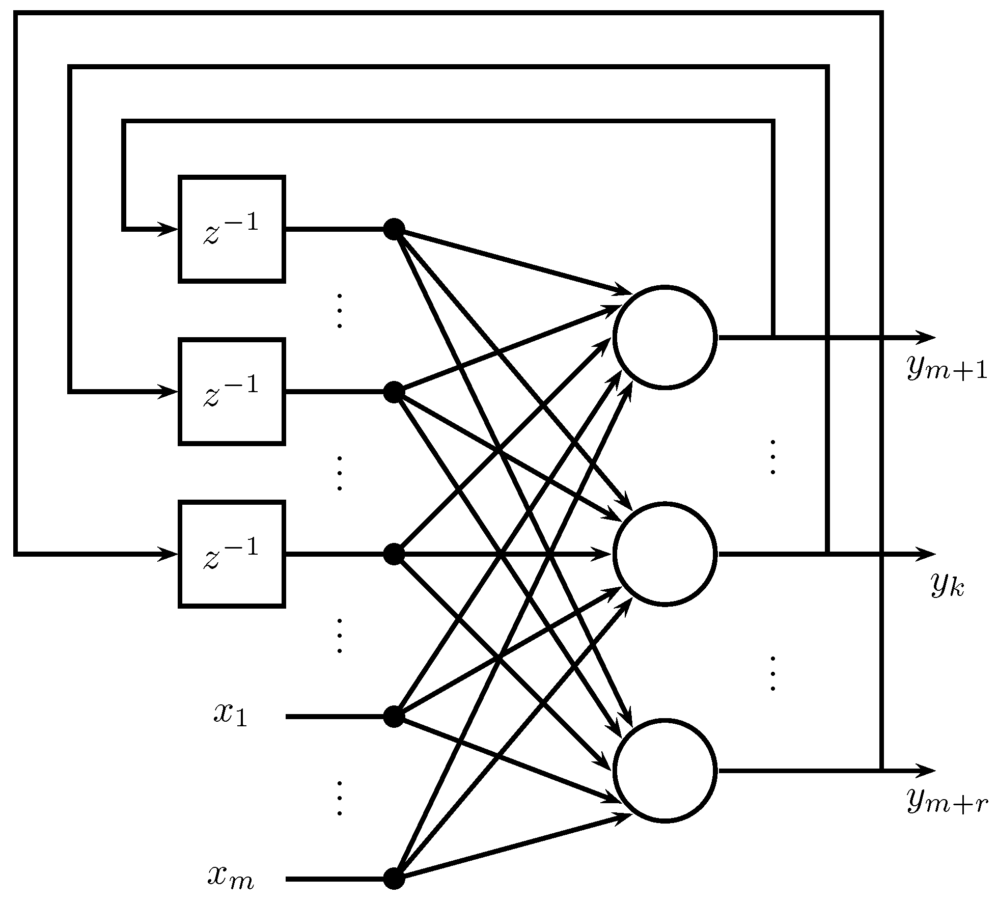
In this paper, is used the RTRL algorithm for the optimization of a fuzzy controller in close-loop, however, to present the RTRL theory is considered the classical application for a Recurrent Network (RN). An example of a fully connected RN is shown in Figure 1, where represents a memory element (delay).
Considering the presented in [15], for a step time n, the parameters of a fully connected recurrent network are:
- : signal applied to input node k.
- : output of processing node k.
- : target output of processing node k.
- : activation of processing node k.
- : weight values connecting node j to node i.
- I: set of indexes associated with the input nodes.
- U: set of indexes associated with the processing nodes.
The neural connections for the output of a processing node k in the step time is , which is calculated using Equation (1).
In Equation (1) is the activation function. On the other hand, taking as the set of indexes belonging to U representing the existence of a target value for a processing node k in a step time n, then, the total instantaneous squared error at the step time n is given by Equation (2).
In Equation (2), the error signal for each node is . Using the gradient descent method where is the learning rate, the weights can be updated using Equation (3).
In this way is observed that:
Calculating the derivative of (given in Equation (1)) with respect to is obtained:
1.4. Proposal Approach and Document Organization
This article shows the optimization of a fuzzy automatic voltage controller for a generation system employing the algorithm real-time recurrent learning. The controller’s optimization is performed in discrete time domain. The architecture of this controller consists of a fuzzy compact structure based on Boolean relations. The main purpose of the document is to deduce the equations of the algorithm for the controller’s training, as well as its application for the AVR system using the weighting values for error and action control obtaining different behaviors. In this way, for the application of generation systems the real-time recurrent learning is a suitable option for training neuro-fuzzy controllers, which is the central aspect of this article.
The main contributions of this work are described as follows.
- Considering a close-loop control system, it is presented the deduction of the training equations employed to implement the training algorithm using the AVR discrete time model. Furthermore, the algorithm steps used for controller optimization are presented.
- Fuzzy controller schemes are proposed making analogies with linear controllers and the result of the training process is shown.
The document is organized as follows. Section 2 details the model of an automatic voltage regulator. Section 3 displays the architecture of the fuzzy controller (compact fuzzy based on Bolean relations). Section 4 presents the deduction of training equations and the algorithm used for parameter adaptation. Next, Section 5 presents the implementation of compact fuzzy controllers: Second Order (SO), PI (Proportional Integral), Proportional Derivative (PD), and Proportional Integral Derivative (PID). Section 6 describes the experimental results; finally, Section 7 presents the conclusions.
2. Automatic Voltage Regulator
In energy systems, the automatic voltage regulator is a crucial part for achieving energy exchange and regulating the energy for the consumers. The AVR in the power system allows supplying quality reliable energy aiming at reducing the steady-state error to zero in an interconnected power system [7]. In the design of an AVR, the main requisites are quick response, low overshoot and steady-state error to zero at deviation from reference voltage [2]; all of this is to keep the reliability in the operations of the power system. Generally, a real power station has more than one generator connected to a busbar and each one has an AVR [16,17].
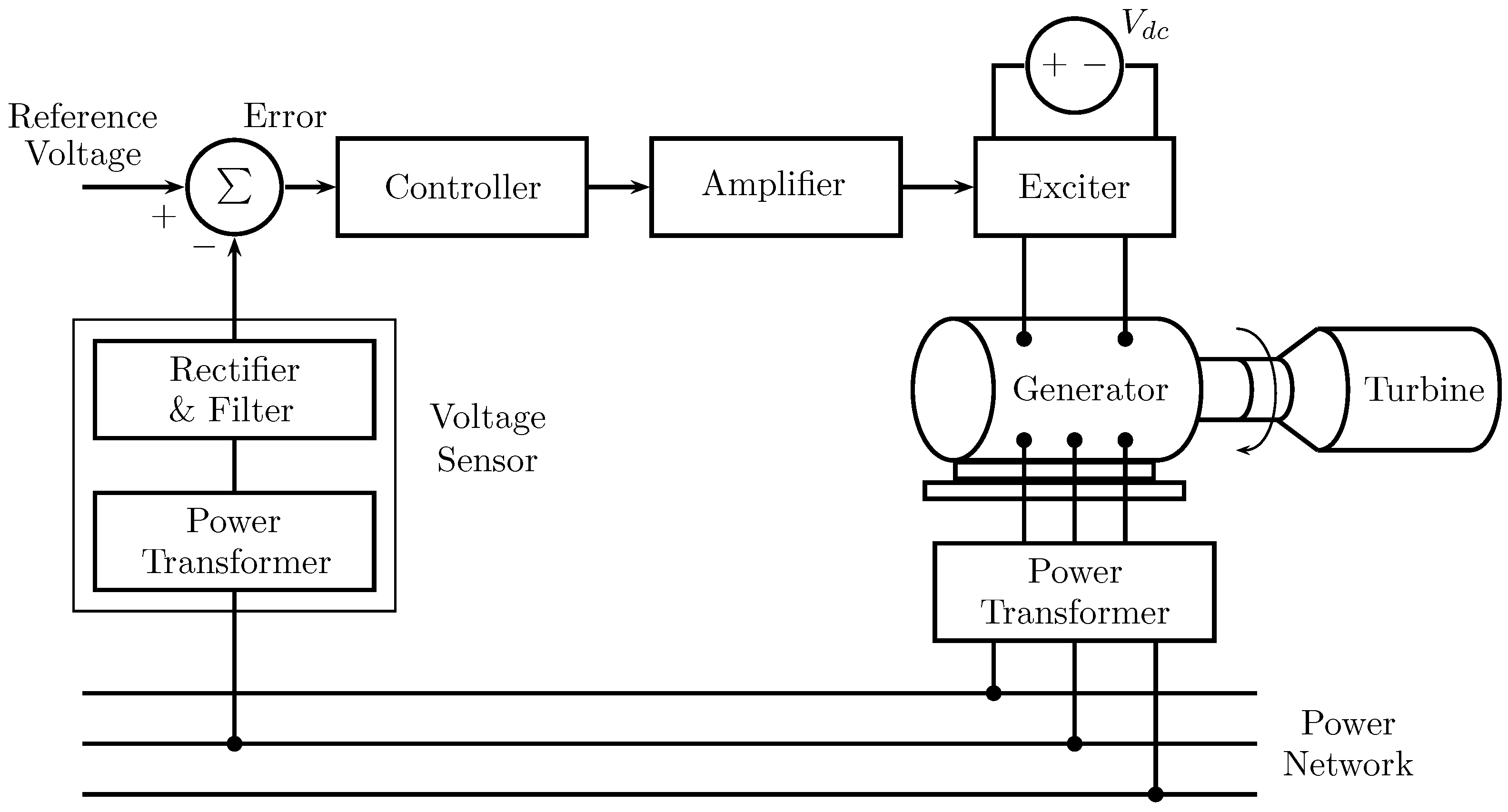
In Figure 2, is observed the schematic diagram of an AVR system. A simple AVR includes four main components: an amplifier, an exciter, a generator, and a sensor [18,19]. In this order, the controller allows having a suitable behavior of AVR.
As mentioned, the purpose of designing an AVR is to keep the output voltage at a certain level in a generation system. An electric power grid includes more than one generator connected to a similar busbar and each one has an AVR. Since the purpose of this system is to control the energy of the power grid to which the generator is connected by a power transformer, the level of energy is constantly measured as a feedback signal using an energy sensor that may consist of a transformer. After being rectified and filtered, this signal is compared to the reference voltage in the comparator to obtain a voltage error signal. The error signal passes through the controller, then it is amplified to feed the exciter for the adjustment of the voltage/current of the field winding in the generator’s in a way that any voltage deviation may be compensated [20].
According to [5], to obtain the mathematical model and transfer function of the AVR, the four main components are linearized taking into account their time constants. Considering the presented in [2,5,21], an AVR can have a representation like the one in Figure 3, where:
- : Amplifier gain (10–40), nominal 10.
- : Excitation gain (1–10), nominal 1.
- : Generator gain (0.7–1.0), depends on the load.
- : Sensor gain with nominal value of 1.
- : Amplifier time constant (0.02 s–0.1 s), nominal .
- : Exciter time constant (0.4 s–1.0 s), nominal .
- : Generator time constant (1.0 s–2.0 s), depends on the load.
- : Sensor time constant (0.001 s–0.06 s), nominal .
AVR Discrete Time Model
Considering that the fuzzy controller optimization takes place in discrete time, it is proceeding to obtain the respective AVR model in this domain. For this, the transfer function of the AVR corresponds to:
Transforming this transfer function into a discrete time representation considering a sampling time of , and using the bilinear transformation method is obtained that:
where . In general, this transfer function can be written as:
Using negative exponents:
3. Fuzzy Controller
According to [22], fuzzy logic has wide applicability in control systems, due to its flexibility for the implementation of control strategies, using knowledge of the system and linguistically proposing control strategies.
The architecture of the fuzzy controller is proposed considering its equivalence with a discrete time linear controller, in this way, the controller is optimized using Real-Time Recurrent Learning.
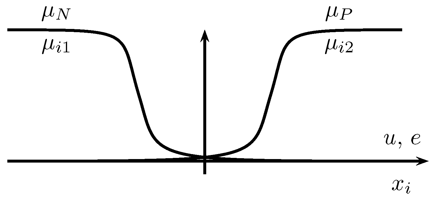
The controller architecture uses the structure of fuzzy logic systems based on Boolean relationships. In this regard, reference [23] presents the design methodology starting from a controller using Boolean sets which then become fuzzy. For the implementation of the fuzzy controller, two possible regions corresponding to negative and positive values in each universe of discourse are considered, therefore, for its implementation, membership functions of the sigmoidal type are used.
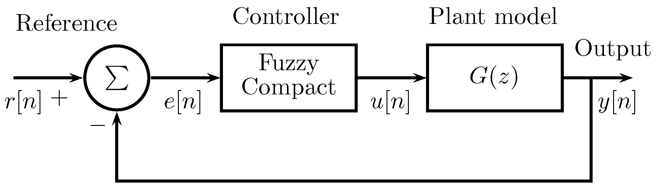
The fuzzy controller uses the compact structure presented in [24] that allows having an equivalence with a linear controller (in discrete time) using fuzzy sets to model the actions of direct inputs and the controller feedback. The general scheme of the control system can be seen in Figure 4.
To carry out the design of the fuzzy controller, a second order linear controller (in discrete time) is considered where the transfer function is:
The difference Equation (in discrete time) of this controller corresponds to:
where the respective coefficients , are constant. For the fuzzy controller, these constants are replaced by non-linear relations given by fuzzy membership functions, such that:
In general terms:
For the fuzzy control system is used the membership functions shown in Figure 5, where fuzzy sets of sigmoidal type are employed to model the negative and positive values of the universe of discourse. In this way, the membership function is given by Equation (17).
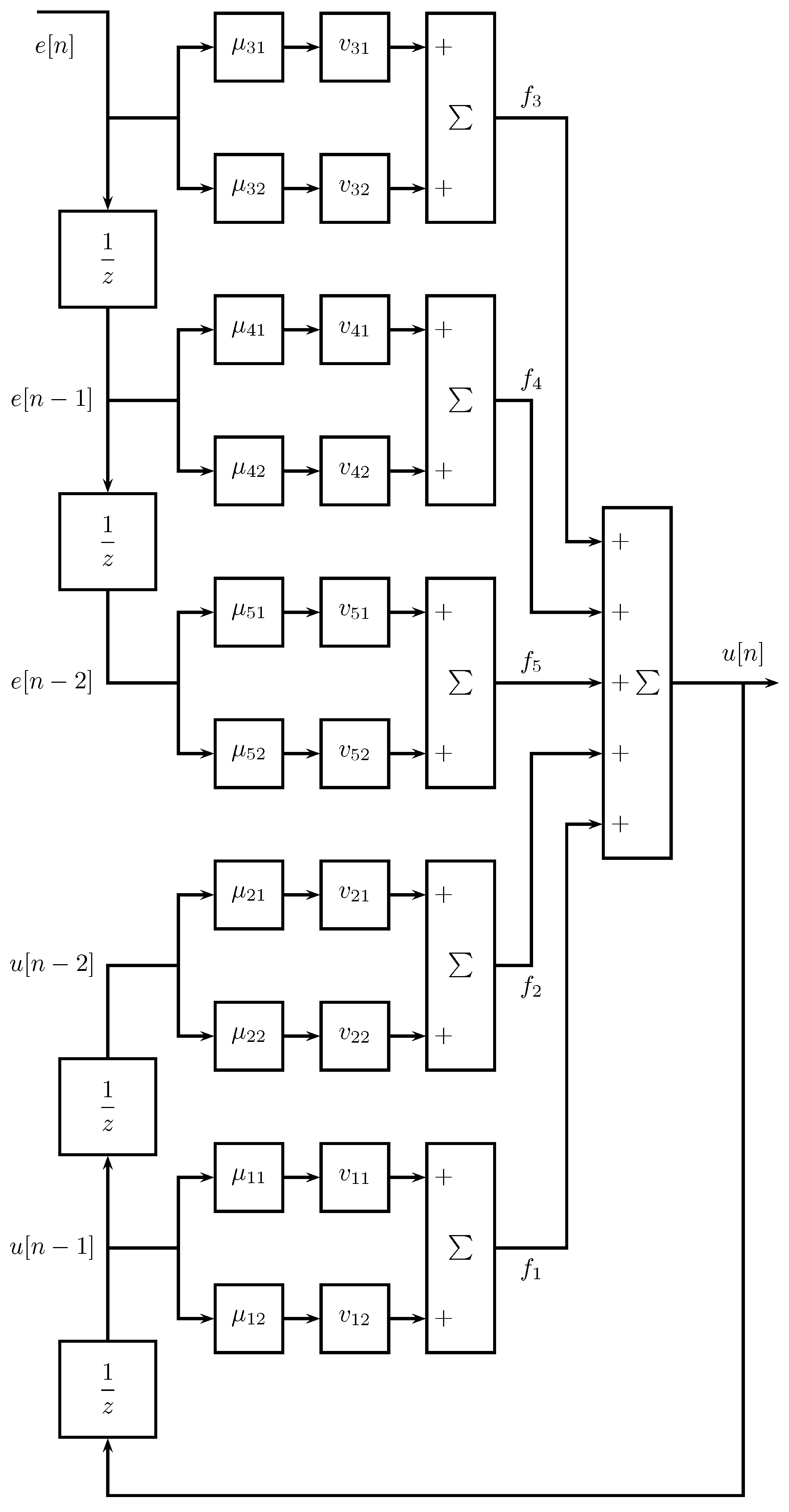
Considering the fuzzy sets of Figure 5, and the general structure of the controller given by the Equation (15) it is obtained the scheme of Figure 6, where the fuzzy controller used is shown.
Considering that , the controller output can be calculated as:
In this way, it is obtained Equation (19), being the set of controller parameters , where is a scalar value and , the parameters of the membership function .
4. Fuzzy Controller Training Process
For a practical approach from the scheme of Figure 3, it is obtained the respective equivalent system in discrete time shown in Figure 4. In this model, the sensor is included as part of the plant, this being the variable to control.
In order to perform the adaptation of the fuzzy controller parameters , it is used the learning rate , if chosen with a very large value, it can cause that the algorithm does not converge, while choosing a very small value can cause the algorithm to require more time to converge [25]. Considering the presented in [25], the training method is based on the direction of maximum descent given by the gradient, therefore, the adaptation (optimization) of is carried out in the following way:
where J corresponds to the adjustment function defined by the error signal then:
In Equation (21) the factor P weights the error signal and Q the control action, in a way that combinations of these values allow having different behaviors as desired.
The derivative of J depending on the adjustment parameters is:
On the other hand, from the transfer function (12), the corresponding recurrence equation for the plant is:
Considering the controller architecture (Figure 6) and Equation (19) for the dynamics of the controller is given by:
To implement the training Equation (20), the derivative of the plant output with respect to a controller parameter is:
In the same way, the derivative of the control action with respect to is:
Meanwhile, the derivative of the error with respect to a controller parameter is:
In order to establish the respective derivatives using Equation (19) is obtained:
where , and , therefore, the following cases are presented:
Case 1: When and j can be equal to any value , then:
The respective derivatives are:
Case 2: When and , it is established that:
Case 3: When and is obtained:
To calculate the respective derivatives of cases 2 and 3, it is first obtained:
For the other derivatives:
In the case of the parameter is determined:
Taking the parameter it is established that:
With the parameter the respective derivative is:
Furthermore, also:
Taking in a general way a controller parameter it has:
Using the previous equations, the update of the controller parameters is carried out using the general Equation (20) having for each parameter the following equations:
Training Algorithm
Algorithm 1 shows the steps used for controller training, in the first step is chosen the initial parameter settings for the controller. In the next step, the control system output is calculated using the plant model. Then it proceeds to perform the adjustment of the fuzzy controller parameters using the equations that involve the dynamics of the control system and the derivatives (Equations (25)–(27) and subsequent equations). It is important to note that the adjusted parameters are stored in an auxiliary variable since during this step the controller does not use these values. Then, it is returned to the step where the control system is evaluated with until complete the simulation time . When completing the simulation time, the controller parameters are updated with the optimized values and it is returned to the step where is calculated the control system response for a new iteration , until the objective function given by Equation (53) is less than a defined , or until k is equal to a defined number .
It should be noted that in this algorithm the AVR discrete time model is used for controller training, therefore, it is not necessary to use additional AVR data. The controller and the plant model are integrated in a control close-loop, in this way, the control system input is the reference desired value .
| Algorithm 1: Training controller. |
 |
5. Implementation of Compact Fuzzy Controllers
The training method is based on the direction of maximum descent given by the gradient, its convergence to the optimum point depends on the initial values of the parameters. Considering that the membership functions used allow representing the actions for positive and negative values, their initial configuration is taken from Figure 5. With this approach, it can be seen that fuzzy systems allow establishing an initial configuration that can be later optimized.
For the design of compact fuzzy controllers, linear control strategies are considered as a reference:
- Second Order Controller (SO).
- Proportional Integral Controller (PI).
- Proportional Derivative Controller (PD).
- Proportional Integral Derivative Controller (PID).
Considering the presented in [24], the compact fuzzy controllers are implemented considering Equation (24) associated with Figure 6, having the following expression:
where . In this way, to establish the equivalence with the discrete time equation of the linear controllers SO, PI, PD, PID, the functions with must be configured as presented below.
5.1. Second Order Controller Structure
The discrete linear controller considered consists of a second order system with transfer function:
The respective difference equation is:
Then for the fuzzy controller is considered the structure:
5.2. PI Equivalent Structure
In this case, the controller has the form:
considering the compact structure it can be expressed as:
In this way, the difference equation of the PI controller corresponds to:
Then for the PI fuzzy controller the structure is:
5.3. PD Equivalent Structure
The PD controller can be represented as:
then the expression for this is:
The corresponding difference equation is:
Then the structure for the PD fuzzy controller is:
5.4. PID Equivalent Structure
In the case of the PID controller, it can be described as:
performing the respective operations it is obtained:
in general, it can be written as:
The respective difference equation for this controller is:
Then for the PID fuzzy controller the structure is:
5.5. Configurations
6. Experimental Results
In order to carry out the experimental tests, it is possible to have different combinations of P and Q, therefore, for the values selection one of these is left fixed, in this case and Q is varied on a logarithmic scale in a way that in the results the effect of these combinations is observed. Furthermore, the learning rate is set to . The values considered of P and Q are the following:
- Case PQ1: , .
- Case PQ2: , .
- Case PQ3: , .
- Case PQ4: , .
The performance index used corresponds to the one shown in Equation (71), where r is the desired output value, y the response of the control system, u the control signal, P and Q weighting values of the error and control action, finally, is the total number of data (total simulation steps).
The process carried out to obtain the experimental results considers the different values of Q and the controllers, thus the steps are:
- (1)
- For each value of Q: , , 1, and 10, do the following:
- (2)
- For each controller: SO, PI, PD, and PID, do the following:
- (3)
- Perform the controller training using Algorithm 1.
- (4)
- Calculate the respective performance index given by Equation (71).
- (5)
- Store the results.
- (6)
- Return to step 2 until completing all controllers.
- (7)
- Return to step 1 until completing all values of Q.
In this way are obtained the results for the values of Q using different compact fuzzy controllers. It should be noted that since the structure and the initial configuration of the controllers given by each is established, only one run of the algorithm is required since the initial configuration is not random. In addition, the reference value since the controller seeks to regulate the normalized output voltage.
The optimization process is performed for the different cases of P and Q for each controller obtaining the results of the objective function shown in Table 2. In this table is seen that when increasing Q the value of the objective function also increases.
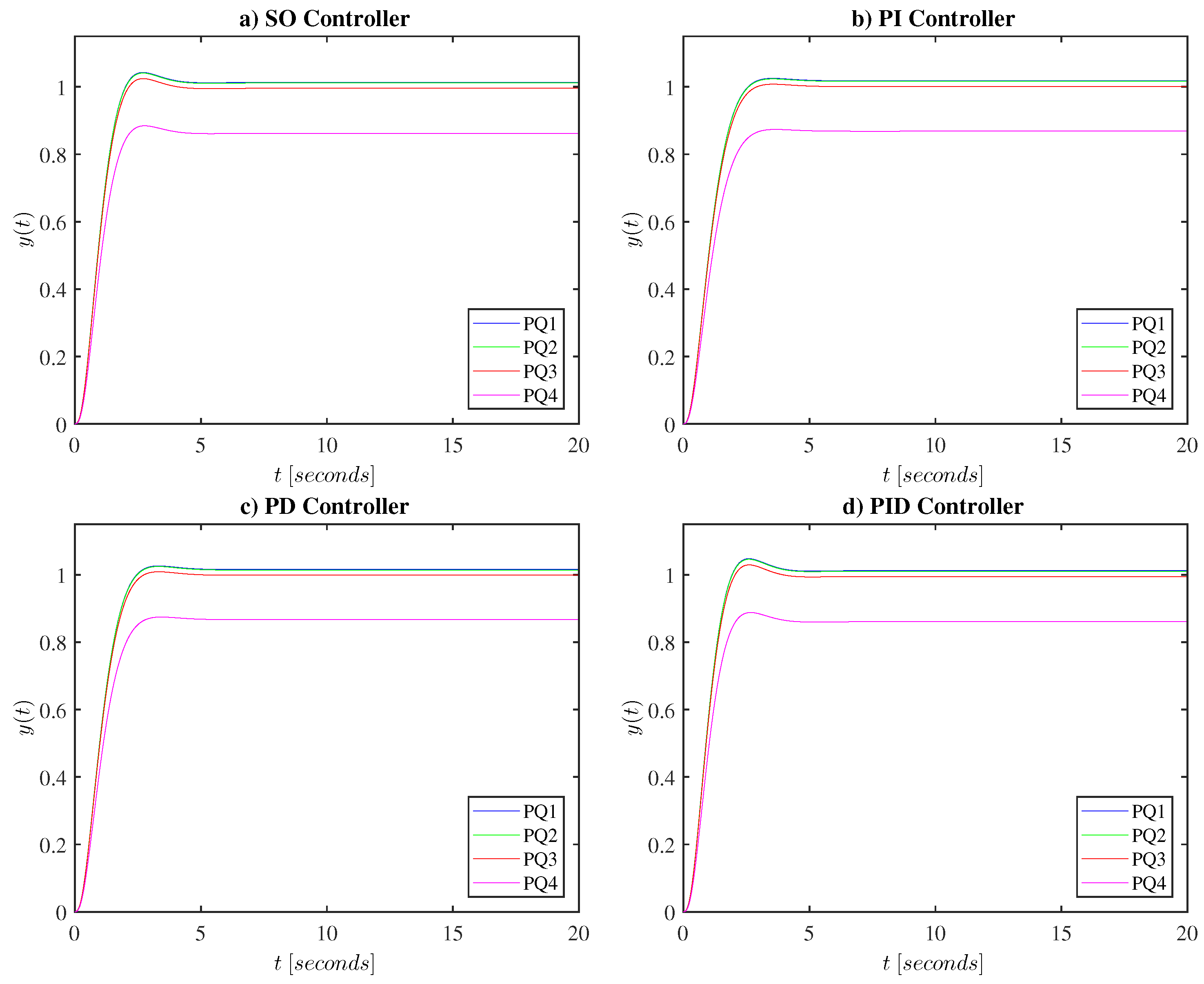
Regarding the performance of the control system, Table 3 shows the performance metrics corresponding to steady state error , overshoot , and settling time . It is to be appreciated that the results with the suitable error in steady state are obtained for the combination of P and Q used in the configuration PQ3. Figure 7, Figure 8 and Figure 9 show the simulations results for the output , control signal , and the objective function .
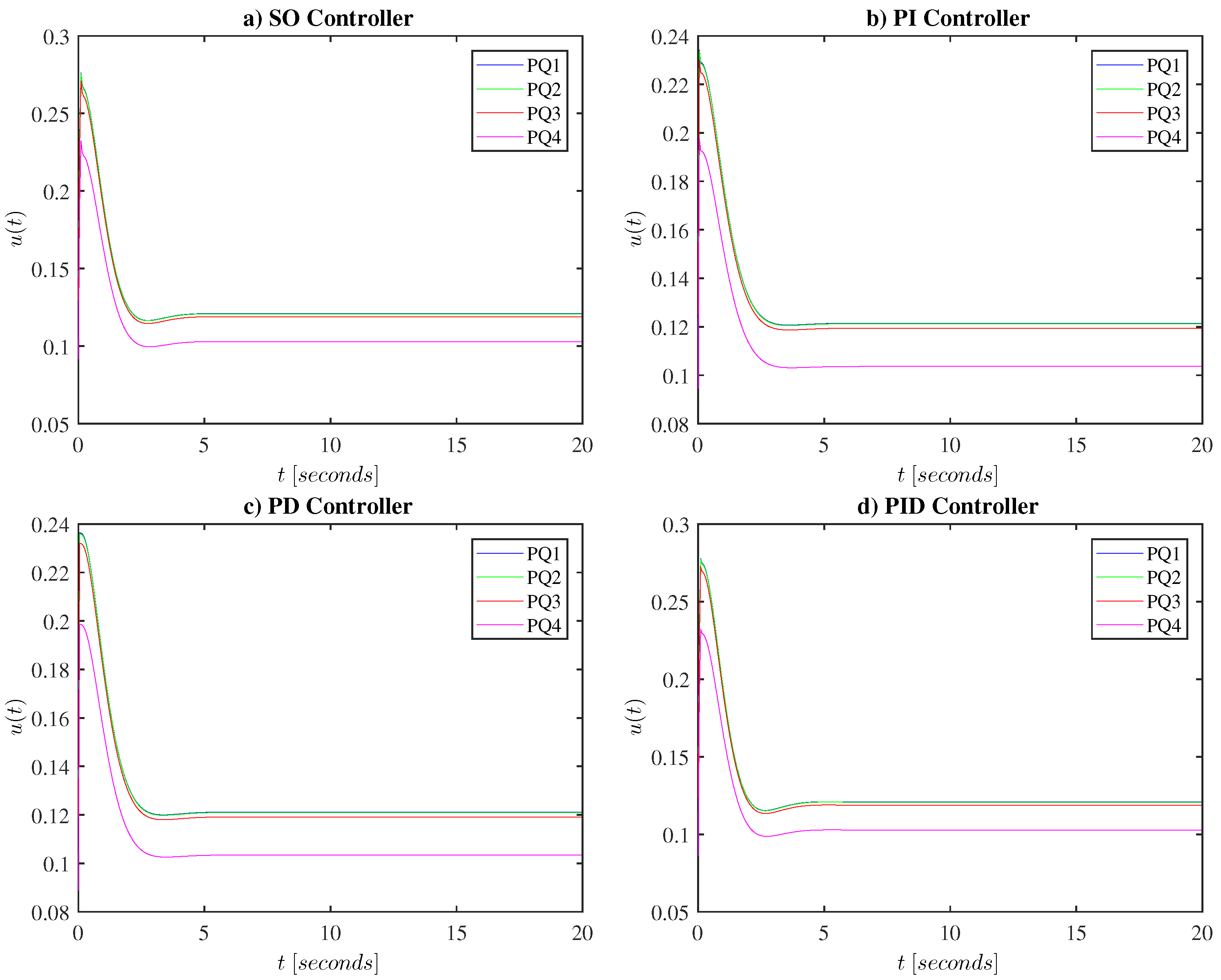
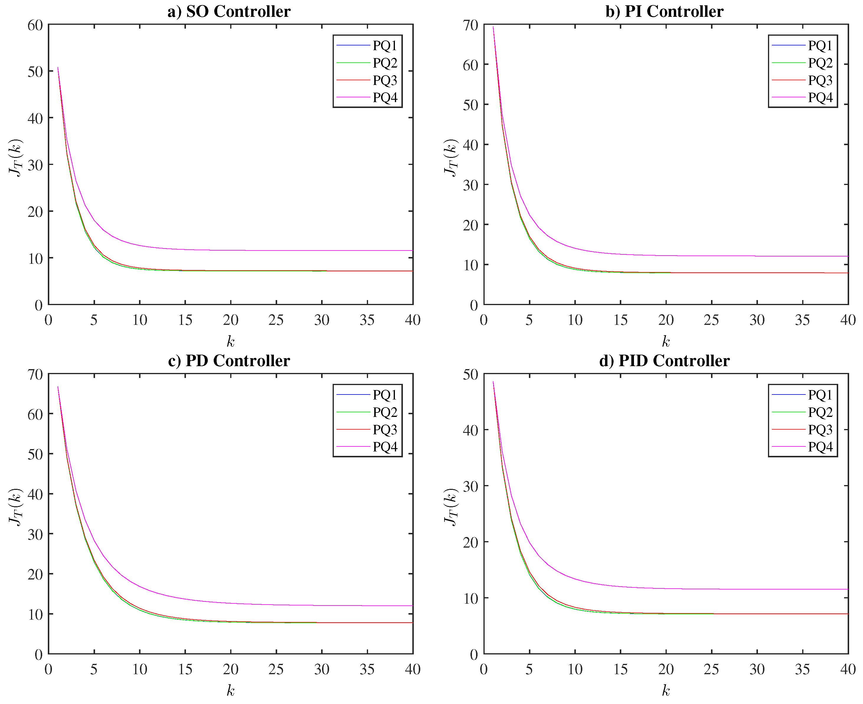
The results of the optimization process for are presented in Figure 7 showing the system’s output with each of the controllers after being optimized. Figure 8 describes the results for the control action observing that when the value of Q increases, the control action decrease. Finally, in Figure 9 is shown the evolution of the training process presenting the values of for each controller considered and the respective setting employed for P and Q.
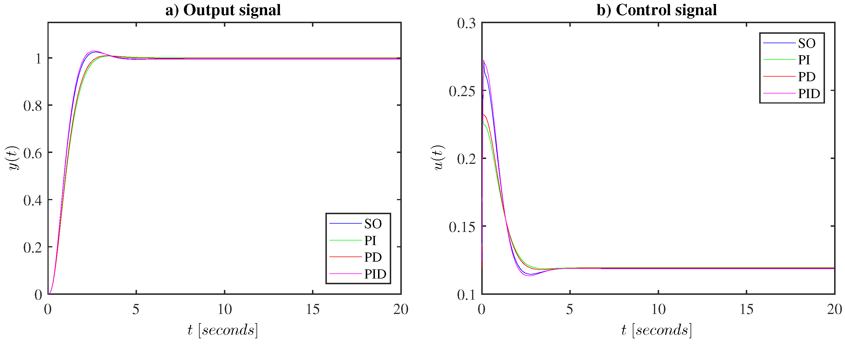
Considering case PQ3, Figure 10 displays the comparison results of controllers SO, PI, PD, and PID presenting the output signal and the control action . In these results, SO has the largest overshot and the PI controller a suitable behavior considering the overshot and setting time.
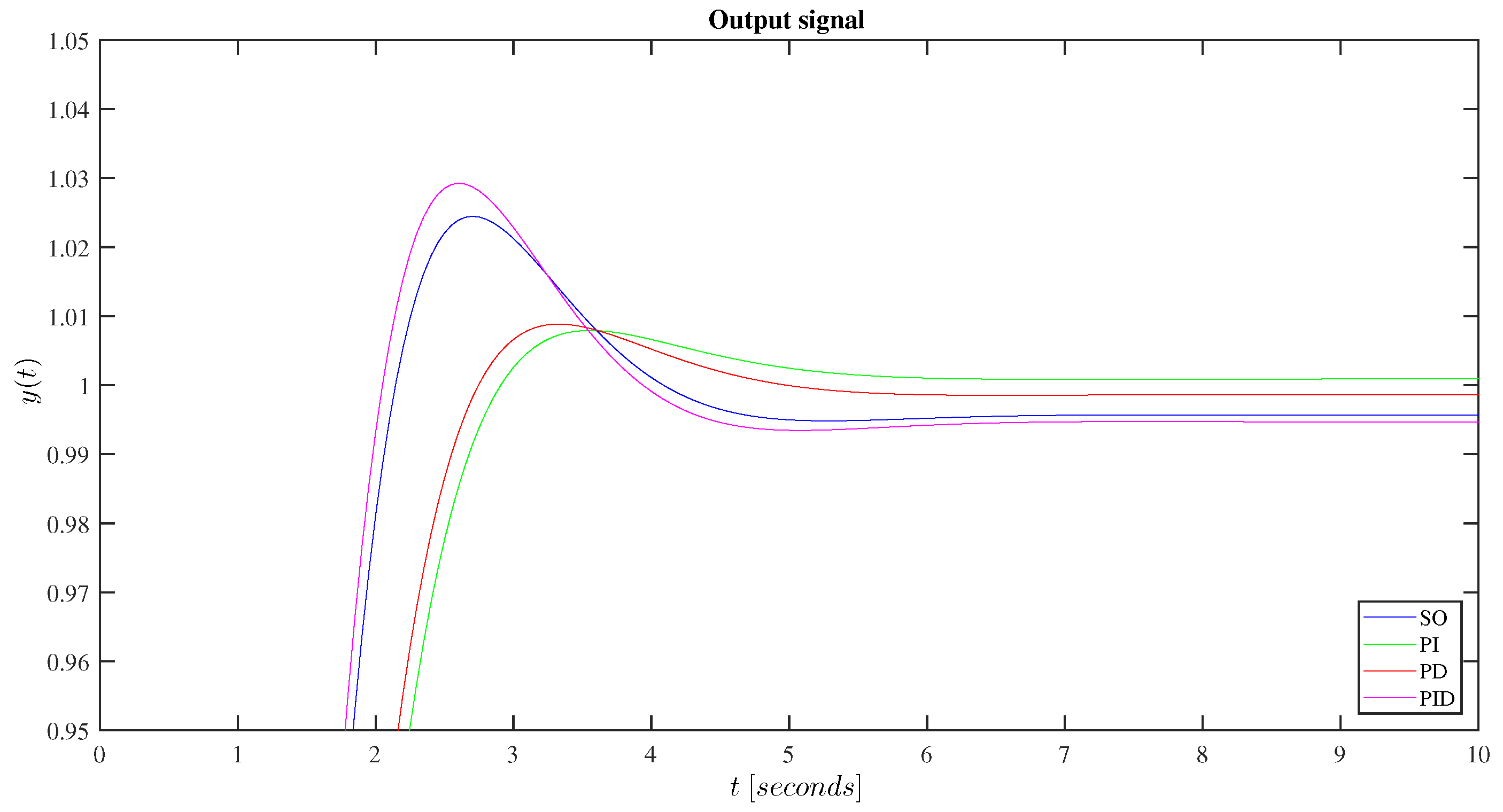
Finally, Figure 11 shows the response detail of the optimized fuzzy controllers, where the steady-state error and the overshoot are better observed for the SO, PI, PD, and PID controllers.
7. Conclusions
In this article, the process for the optimization of an automatic voltage controller using Real-Time Recurrent Learning was presented, making the deduction of the respective equations used for the implementation of this algorithm.
In order to carry out the experimental tests, different configurations for the P and Q values are considered; P weights the error signal and Q the control action, in a way that combinations of these values allow having different behaviors.
The results show the response of the different fuzzy controllers considered which were determined by the analogy of linear controllers, namely, base on preliminary knowledge of the controllers, therefore the controller topology considered was SO, PI, PD, PID.
The configurations display different dynamic behaviors according to values of P and Q. Checking the results, the control action decreases when the value of Q increases.
The record of the objective function in each of the cases considered shows that the optimization process is successful using the deduced equations.
This scheme can be used to tune the controller in real time with an adaptive scheme when there are variations in the plant. Besides, in an additional work other fuzzy controller configurations could be used.
Author Contributions
Conceptualization, H.E., I.M. and H.L.; Methodology, H.E., I.M. and H.L.; Project administration, H.L.; Supervision, H.L.; Validation, I.M.; Writing—original draft, H.E.; Writing—review and editing, H.E., I.M. and H.L. All authors have read and agreed to the published version of the manuscript.
Funding
This research received no external funding.
Institutional Review Board Statement
In this work were not carried out test on individuals (humans).
Informed Consent Statement
The study presented in this work does not involve human beings.
Data Availability Statement
No external data were required for this work.
Acknowledgments
The authors express gratitude to the Universidad de Oviedo, and the Universidad Distrital Francisco José de Caldas.
Conflicts of Interest
The authors declare no conflict of interest.
References
- Mohamed, T.H.; Mohammed, A.; Abd-Eltawwab, A.; Hiyama, T. Wide-area Power System Oscillation Damping using Model Predictive Control Technique. IEEJ Trans. Power Energy 2011, 131, 536–541. [Google Scholar] [CrossRef]
- Liu, Q.; Mohamed, T.; Kerdphol, T.; Mitani, Y. PID-MPC Based Automatic Voltage Regultaor Design in Wide-Area Interconected Power System. Int. J. Emerg. Technol. Adv. Eng. 2014, 4, 412–417. [Google Scholar]
- Holt, M.; Rehtanz, C. Optimizing line-voltage-regulators with regard to power quality. Electr. Power Syst. Res. 2021, 190, 106654. [Google Scholar] [CrossRef]
- Calderón, J.G.; Castellanos, R.; Ramirez, M. Stability Enhancement of an Industrial Power System by AVR Gain Readjustment. IEEE Lat. Am. Trans. 2017, 15, 663–668. [Google Scholar] [CrossRef]
- Bhatt, V.; Bhongade, S. Design Of PID Controller In Automatic Voltage Regulator (AVR) System Using PSO Technique. Int. J. Eng. Res. Appl. (IJERA) 2013, 3, 1480–1485. [Google Scholar]
- D’Agostino, F.; Kaza, D.; Martelli, M.; Schiapparelli, G.P.; Silvestro, F.; Soldano, C. Development of a Multiphysics Real-Time Simulator for Model-Based Design of a DC Shipboard Microgrid. Energies 2020, 13, 3580. [Google Scholar] [CrossRef]
- Musa, B.U.; Kalli, B.M.; Shettima, K. Modeling and Simulation of Lfc and Aver with PID Controller. Int. J. Eng. Sci. Invent. 2013, 2, 54–57. [Google Scholar]
- Park, C.-Y.; Kwon, J.-M.; Kwon, B.-H. Automatic voltage regulator based on series voltage compensation with ac chopper. IET Power Electron. 2012, 5, 719–725. [Google Scholar] [CrossRef]
- Khan, I.A.; Alghamdi, A.S.; Jumani, T.A.; Alamgir, A.; Awan, A.B.; Khidrani, A. Salp Swarm Optimization Algorithm-Based Fractional Order PID Controller for Dynamic Response and Stability Enhancement of an Automatic Voltage Regulator System. Electronics 2019, 8, 1472. [Google Scholar] [CrossRef] [Green Version]
- Micev, M.; Calasan, M.; Oliva, D. Fractional Order PID Controller Design for an AVR System Using Chaotic Yellow Saddle Goatfish Algorithm. Mathematics 2020, 8, 1182. [Google Scholar] [CrossRef]
- Sikander, A.; Thakur, P. A new control design strategy for automatic voltage regulator in power system. ISA Trans. 2020, 100, 235–243. [Google Scholar] [CrossRef] [PubMed]
- Micev, M.; Ćalasan, M.; Ali, Z.M.; Hasanien, H.M.; Abdel Aleem, S.H.E. Optimal design of automatic voltage regulation controller using hybrid simulated annealing—Manta ray foraging optimization algorithm. Ain Shams Eng. J. 2021, 12, 641–657. [Google Scholar] [CrossRef]
- Du, K.L.; Swamy, M.N.S. Neural Networks and Statistical Learning; Springer: London, UK, 2013. [Google Scholar]
- Singh, M.; Singh, I.; Verma, A. Identification on Non Linear Series-Parallel Model Using Neural Network. MIT Int. J. Electr. Instrum. Eng. 2013, 3, 21–23. [Google Scholar]
- Mak, M.W.; Ku, K.W.; Lu, Y.L. On the improvement of the real time recurrent learning algorithm for recurrent neural networks. Neurocomputing 1999, 24, 13–36. [Google Scholar] [CrossRef]
- Khalil, A.; Peng, A.S. An Accurate Method for Delay Margin Computation for Power System Stability. Energies 2018, 11, 3466. [Google Scholar] [CrossRef] [Green Version]
- Machowski, J.; Lubosny, Z.; Bialek, J.W.; Bumby, J.R. Power System Dynamics: Stability and Control, 3rd ed.; John Wiley & Sons: West Sussex, UK, 2020. [Google Scholar]
- Shayeghi, H.; Dadashpour, J. Anarchic Society Optimization Based PID Control of an Automatic Voltage Regulator (AVR) System. Electr. Electron. Eng. 2012, 2, 199–207. [Google Scholar] [CrossRef] [Green Version]
- Modabbernia, M.; Alizadeh, B.; Sahab, A.; Moghaddam, M.M. Robust control of automatic voltage regulator (AVR) with real structured parametric uncertainties based on H∞ and μ-analysis. ISA Trans. 2020, 100, 46–62. [Google Scholar] [CrossRef]
- Çelik, E.; Durgut, R. Performance enhancement of automatic voltage regulator by modified cost function and symbiotic organisms search algorithm. Eng. Sci. Technol. Int. J. 2018, 21, 1104–1111. [Google Scholar] [CrossRef]
- Gaing, Z.L. A particle swarm optimization approach for optimum design of PID controller in AVR system. IEEE Trans. Energy Convers. 2004, 19, 384–391. [Google Scholar] [CrossRef] [Green Version]
- Rajasekaran, S.; Pai, G.A.V. Neural Networks, Fuzzy Systems and Evolutionary Algorithms: Synthesis and Applications; PHI Learning Private Limited: Delhi, India, 2017. [Google Scholar]
- Espitia, H.; Soriano, J.; Machón, I.; López, H. Design Methodology for the Implementation of Fuzzy Inference Systems Based on Boolean Relations. Electronics 2019, 8, 1243. [Google Scholar] [CrossRef] [Green Version]
- Espitia, H.; Soriano, J.; Machón, I.; López, H. Compact Fuzzy Systems Based on Boolean Relations. Appl. Sci. 2021, 11, 1793. [Google Scholar] [CrossRef]
- Chow, T.W.S.; Cho, S.Y. Neural Networks and Computing: Learning Algorithms and Applications; Series in Electrical and Computer Engineering; Imperial College Press: London, UK, 2007; Volume 7. [Google Scholar]
Figure 1.
Example of a fully connected recurrent neural network using m inputs, and r processing nodes.
Figure 1.
Example of a fully connected recurrent neural network using m inputs, and r processing nodes.

Figure 2.
Schematic diagram of an AVR system.

Figure 3.
Block diagram of the AVR system.

Figure 4.
General diagram of the control system.

Figure 5.
Membership functions used.

Figure 6.
Fuzzy control system scheme.

Figure 7.
Optimization process results for the output .

Figure 8.
Optimization process results for the control action .

Figure 9.
Optimization process results for the objective function .

Figure 10.
Results of and for case PQ3.

Figure 11.
Detail results of for case PQ3.


Table 1.
Compact fuzzy controller configurations.
| Controller | |||||
|---|---|---|---|---|---|
| SO | Yes | Yes | Yes | Yes | Yes |
| PI | Yes | No | Yes | Yes | No |
| PD | No | No | Yes | Yes | No |
| PID | Yes | No | Yes | Yes | Yes |
Table 2.
Results of the optimization process.
| Configuration | PQ1 | PQ2 | PQ3 | PQ4 |
|---|---|---|---|---|
| SO | 7.1560 | 7.1572 | 7.2216 | 11.5680 |
| PI | 7.8564 | 7.8576 | 7.9196 | 12.1120 |
| PD | 7.7172 | 7.7192 | 7.7880 | 12.0156 |
| PID | 7.0820 | 7.0832 | 7.1488 | 11.5252 |
Table 3.
Performance metrics.
| Configuration | PQ1 | PQ2 | PQ3 | PQ4 | ||||||||
|---|---|---|---|---|---|---|---|---|---|---|---|---|
| Metric | ||||||||||||
| SO | 1.3016 | 2.92270 | 3.2624 | 1.1415 | 2.91970 | 3.2623 | 0.43209 | 2.8901 | 3.2610 | 13.8212 | 2.6418 | 3.2444 |
| PI | 1.7971 | 0.71551 | 2.5343 | 1.6394 | 0.71433 | 2.5349 | 0.08932 | 0.7026 | 2.5411 | 13.1534 | 0.60214 | 2.599 |
| PD | 1.5554 | 1.03820 | 2.3977 | 1.3994 | 1.03660 | 2.3983 | 0.13611 | 1.0215 | 2.4045 | 13.3099 | 0.8858 | 2.4640 |
| PID | 1.2032 | 3.51250 | 3.2928 | 1.0429 | 3.50910 | 3.2928 | 0.53243 | 3.4747 | 3.2934 | 13.9399 | 3.182 | 3.29510 |
Publisher’s Note: MDPI stays neutral with regard to jurisdictional claims in published maps and institutional affiliations. |
© 2021 by the authors. Licensee MDPI, Basel, Switzerland. This article is an open access article distributed under the terms and conditions of the Creative Commons Attribution (CC BY) license (https://creativecommons.org/licenses/by/4.0/).
Share and Cite
MDPI and ACS Style
Espitia, H.; Machón, I.; López, H. Optimization of a Fuzzy Automatic Voltage Controller Using Real-Time Recurrent Learning. Processes 2021, 9, 947. https://0-doi-org.brum.beds.ac.uk/10.3390/pr9060947
AMA Style
Espitia H, Machón I, López H. Optimization of a Fuzzy Automatic Voltage Controller Using Real-Time Recurrent Learning. Processes. 2021; 9(6):947. https://0-doi-org.brum.beds.ac.uk/10.3390/pr9060947
Chicago/Turabian StyleEspitia, Helbert, Iván Machón, and Hilario López. 2021. "Optimization of a Fuzzy Automatic Voltage Controller Using Real-Time Recurrent Learning" Processes 9, no. 6: 947. https://0-doi-org.brum.beds.ac.uk/10.3390/pr9060947
Note that from the first issue of 2016, this journal uses article numbers instead of page numbers. See further details here.