CFD Performance Analysis of a Dish-Stirling System for Microgeneration

Abstract

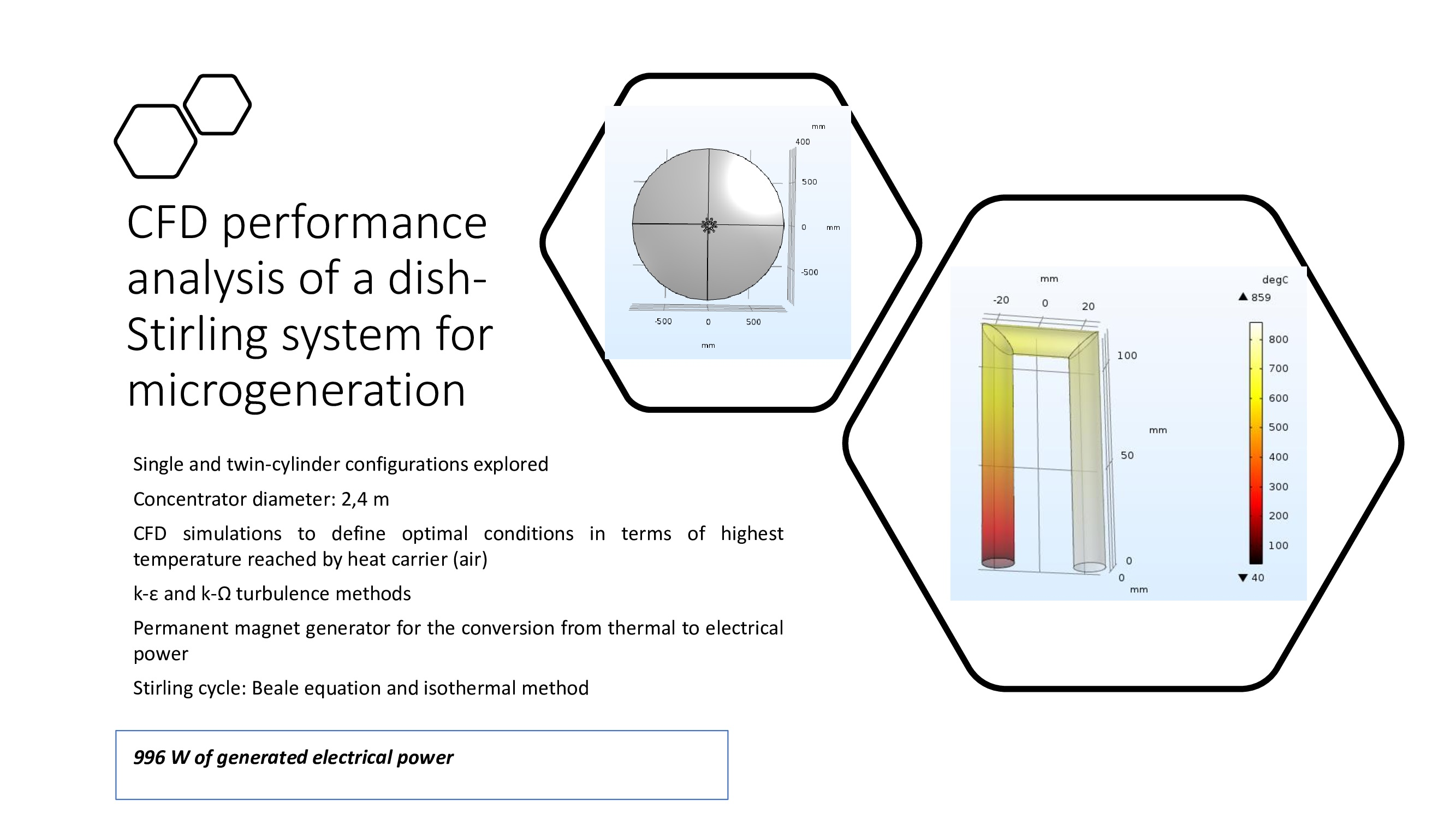
The sustainable transition towards renewable energy sources has become increasingly important nowadays. In this work, a microgeneration energy system was investigated. The system is composed of a solar concentrator system coupled with an alpha-type Stirling engine. The aim was to maximize the production of electrical energy. By imposing a mean value of the direct irradiance on the system, the model developed can obtain the temperature of the fluid contained inside the Stirling engine. The heat exchanger of the microgenerator system was analyzed, focusing on the solar coupling with the engine, with a multiphysical approach (COMSOL v5.3). A real Stirling cycle was implemented using two methods for comparison: the first-order empirical Beale equation and the Schmidt isothermal method. Results demonstrated that a concentrator of 2.4 m in diameter can generate, starting from 800 W/m² of mean irradiance, a value of electrical energy equal to 0.99 kWe.

1. Introduction

The depletion of fossil sources and the environmental crisis has worsened over the years and has led to an inevitable transition towards the exploitation of renewable energy sources. Figure 1 demonstrates a six-fold increase of global investment in renewable energies from 2004–2014 [1].

The most important renewable energy source comes from the sun, which can be used to produce energy through various technologies which are constantly improved. The development of solar-based systems is important for greater security and independence, and the environmental impacts are limited [3]. The exploitation of concentrating systems is more advantageous than other solar technologies for energy generation [4]. Recent updates involve the coupling of concentrated solar power systems with Micro Gas Turbines (MGT) for a technology linked to new small high-temperature solar receivers [5], as opposed to the Stirling technology which is already considered an established technology. Solar energy is not only useful to produce electrical energy but also for recent technologies such as “photovoltaic powered reverse osmosis” (PV-RO) and “solar thermal powered reverse osmosis” (ST-RO) which can sustainably perform desalination [6].

The solar source is not constant, it is a function of the position of the solar concentrator in terms of latitude, longitude, and the consequent “Direct Normal Irradiance” [7]. This value can be measured with a pyrheliometer mounted on the solar concentrator [8]. Figure 2 shows the different techniques to exploit the solar source which have been developed recently [9]. The integration of systems such as photovoltaic panels and CSP systems into power grids represents a remarkable application that could significantly increase the ability to generate sustainable electrical power [9,10].

Most of the systems presented refer to indirect systems using thermodynamic cycles.

Islam et al., (2018) investigated solar technologies and found that the most promising choice considers a thermodynamic cycle coupled with an electrical generation system [11]. Molten salts are the most commonly used thermal fluids [12,13]. An example of large-scale applied solar technologies is the “Solana Generating Station”, completed in 2013 in Arizona (USA) [14]. The plant includes a 280 MW parabolic trough solar plant that can provide energy for up to 70,000 households in the Arizona area [15].

Air Brayton cycles and supercritical CO₂ Brayton cycles were investigated in pilot plant case studies [16,17].

An example of Stirling cycle technology is the EuroDISH, a system that can produce up to 10 kW of electrical energy with a concentrator of 7.5 m in diameter. The system is shown in Figure 3 and can be found at the “Plataforma Solar de Almería” in Almería, Spain [18,19].

Another dish-Stirling cycle was built in Jodhpur (India), with a 50 MW CSP system. This station is composed of 2000 units of the parabolic dish-Stirling, each having 25 kWe capacity [20]. This aspect highlights the modularity of such technologies.

Another current example of valid application of the dish-Stirling is for the absorption and compression of cooling systems. Current works [21] show that compression systems are able to produce up to 53% of cooling power more than the amount of heat supplied.

The second main component of the dish-Stirling is the Stirling engine, an external combustion engine with two separate cylinders on the expansion side and the compression side. The space between the hot and cold side of the engine is called “regenerator” and acts as a heat recuperator to reduce the work of the compression and expansion of the pistons [22].

Since this type of engine is an external combustion engine, it can be fed by various kinds of external heat sources: fuel, solar, geothermal, or waste heat [23]. The heat source hits the walls of the hot side heat exchanger, inside which the heat carrier fluid reaches a sufficient temperature level to start the Stirling cycle. The continuous heating and refrigerating of the heat carrier inside the two cylinders are crucial for the continuation of the cycle [24].

This project focuses on the Stirling cycle fed by solar energy through a solar dish concentrator. The solar concentrator focuses the “Direct Normal Irradiance”, DNI, on a plane called the “focal plane”. On this plane, an α-Stirling engine uses this energy to heat its fluid carrier contained inside the engine and initiates the Stirling cycle to generate electrical power.

This article aims to evaluate the electrical production of renewable energy thanks to dish-Stirling technology. The project will consider two different configurations, while the highest performances will be chosen. The starting point for the simulation is the Direct Normal Irradiance (DNI), values obtained from the Politecnico di Torino tracking system. This average value is typically measured in hotter seasons (spring and summer).

Following the same principle, the most suitable material in terms of temperature reached by the heat carrier fluid inside the pipe of the exchanger was evaluated experimentally. After deciding the most suitable material between the two materials presented, the temperature of the fluid was used to simulate a Stirling cycle, with constant electrical power production. In the end, this value will be compared with lower values of DNI, typical of colder seasons such as winter and autumn.

2. Geometry and Design Parameters of the System

The solar concentrator used in the project is mounted on the roof of Politecnico di Torino (Energy Center). The solar concentrator was built by El.Ma. Electronic Machining srl (TN, Italy). The geometrical data used for the simulation of geometric optics are reported in

Table 1. Parameters of the solar dish concentrator.

Name	Value	Description
f	0.92 m	Focal length
phi	0.9028 rad	Rim angle
d	2.4 m	Dish diameter
A	4.48 m2	Dish projected surface area
psim	0.00465 rad	Maximum solar disc angle

presented below:

These parameters can be implemented in the COMSOL Multiphysics 5.3 library, in which it is possible to create the geometry of a parabolic concentrator with negligible thickness for the Ray Tracing analysis. The geometry of the concentrator is shown in Figure 4 [19], the rim angle can be calculated from focal length and dish diameter:

$$d=4·f·\left[\csc \left(\phi \right)-\cot \left(\phi \right)\right]=2.4 \mathrm{m}$$

(1)

As far as the mean irradiation value is concerned, a constant initial value was chosen for the simulation. This parameter can be measured by the concentrator through a pyrheliometer mounted on the concentrator. The average value defined for the simulation is 800 W/m². This value is mainly measured during hotter seasons of the year, while for autumn and winter, the values tend to decrease slightly.

The hot side heat exchanger is the area of the engine which receives the concentrated energy and, for this project, the geometry for the heat exchanger was developed using CAD software SolidWorks 2019, whereas the CFD simulations were carried out using COMSOL Multiphysics 5.3. The presented work follows the following steps: the analysis of the two chosen configurations for the engine between the single-cylinder and the twin-cylinder. Next, another CFD simulation was implemented to choose the most suitable material for the hot heat exchanger between AISI 310 and Inconel 625, both of which show high resistance at high temperatures. Lastly, the third and final simulation allows to find the desired value of temperature reached by the fluid inside the engine. This is an important value used to simulate a real Stirling cycle with two methods: the first-order empirical method known as “Beale equation” and the second-order method known as “Schmidt analysis” to evaluate the heat power produced which, by coupling the system with a permanent magnet generator gives the final result: the electrical power output of the system.

The Stirling engine chosen for the project is designed by an Italian Stirling engine manufacturer “Genoastirling s.r.l.”. An example of this engine is shown in Figure 5 in both the single-cylinder (ML1000) and twin-cylinder configuration (ML3000).

The engine designed by Genoastirling is an alpha-type engine that uses air as a heat carrier throughout the cycle. The cold temperature for the Stirling cycle is 40 °C and the objective of this article is to evaluate the hot temperature reached by the fluid for the analysis of power production. In

Table 2. Parameters of the engine.

Parameters	Value	Unit of Measurement
Geometric Parameters
Connecting rod length	210	mm
Diameter of the cylinder	110	mm
Cylinder stroke	55.2	mm
Offset compression-expansion cycle	90	sexagesimal degree °
Compression cylinder displacement	524.6	cm3
Expansion cylinder displacement	524.6	cm3
Compression cylinder dead volume	153.3	cm3
Expansion cylinder dead volume	153.3	cm3
Operative Parameters
Rotational speed	600	rpm
Working fluid	Air	-
Average pressure indicated	15	bar
Cooling fluid	Water	-
Hot side starting temperature	700	°C

, the main geometric and operative parameters of the engine can be found.

The engine’s hot side heat exchanger is placed on the focal plane and receives the energy from the concentrator on its external surface. The receiver is therefore represented by the entire surface of the hot side heat exchanger and has to be designed to be implemented in COMSOL Multiphysics 5.3 through the function “LiveLink for SolidWorks”. The heat exchanger for the hot side is called “Nazgul” and a model of the exchanger created using SolidWorks version 2019 is shown in Figure 6 with the technical parameters defined in

Table 3. Characteristics of the Nazgul heat exchanger.

Technical Data for the Exchanger
Number of pipes	9
External diameter (mm)	20
Internal diameter (mm)	14
Pipe thickness (mm)	3
Max pipe height (mm)	120
Twin-cylinder exchangers’ center distance (mm)	274

.

By knowing all the technical details of the heat exchanger, the model of the system was developed and implemented in COMSOL Multiphysics for the Ray Tracing simulation to decide the most suitable configuration between the single and the twin-cylinder. The resulting geometries for the two distinct simulations are presented in Figure 7.

By implementing the various deviations from the ideal concentration such as the absorption coefficient equal to 0.15 and the optical limitations of the mirror with a “limb darkening” model coupled with a surface roughness of 1.75 microns, the simulation has been successfully run. The analysis for the results is based on the Stefan–Boltzmann law, where σ is the Stefan–Boltzmann coefficient equal to 5.67 × 10⁻⁸ W/(m²K⁴):

$$T={\left(\frac{q}{\sigma }\right)}^{0.25}$$

(2)

The parameter defined in Equation (2) as “q” can be defined in COMSOL 5.3 as the heat source at the wall (W/m²), and the results obtained for the two temperature profiles with the single-cylinder and the twin-cylinder engine configurations are shown respectively in Figure 8a,b.

Figure 8 show that the higher encumbrance of the twin-cylinder engine results in a poorer temperature distribution along the external surface of the heat exchanger and a lower overall average temperature. The maximum reachable temperature in the single-cylinder configuration reaches a value of around 900 °C, this value drops down to 740 °C for the twin-cylinder. For these reasons, the choice for the continuation of the project is the single-cylinder one given the higher performances obtained by such configuration. The simulation also allows to obtain the value of “average heat source at the wall” which, for this specific case, is equal to 5990 W/m².

3. Materials

Having obtained the configuration for the system, it is important to evaluate the two proposed materials for the hot side heat exchanger. The materials taken into consideration for the simulation are AISI 310 and Inconel 625, both of which are proven to be highly resistant at high temperatures. These materials are resistant to temperatures above 1000 °C, therefore, are both suitable for the application since the system does not reach temperatures higher than 920 °C. The characteristics of the two materials at high temperature are defined in

Table 4. Physical parameters for the materials.

Physical Properties	AISI 310	Inconel 625
Density (kg/m3)	7550	8440
Heat capacity at constant pressure (J/kg/K)	610	560
Thermal conductivity (W/m/K)	23.7	20.3

.

The second simulation is performed to choose the most suitable material in terms of reached temperature on the internal pipe, which represents the solid–fluid interface for the Stirling engine.

The external tube’s temperature is equal to the external temperature (20 °C), and the simulation is a transitory heat exchange in solids. The objective is to comparatively evaluate the material that can guarantee the highest temperature with an equal time. The geometry inevitably considers the width of the pipe equal to 3 cm and the model used for the simulation is shown in Figure 9.

4. Results

4.1. Temperature Distribution

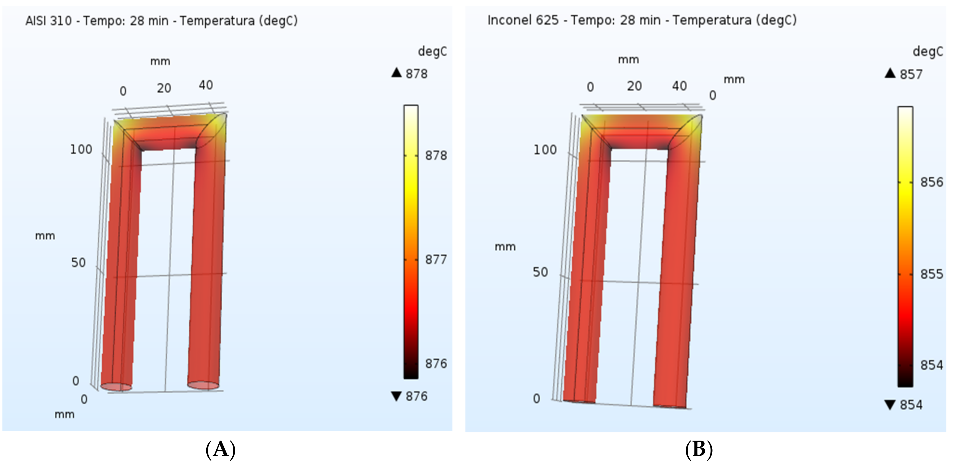
The parameter chosen as input for the simulation is the average heat source at the wall equal to 5990 W/m² previously calculated. The results are presented in Figure 10 and show AISI 310 and Inconel 625 and their temperature profile at a constant time value of 28 min. A fixed time value was chosen to evaluate which material can guarantee a higher temperature on the internal side of the pipe. The value settled for both simulations with AISI 310 and Inconel 625 is 28 min. Figure 11 shows the difference in the temperature profile between the two materials at the same fixed time value. This was decided to choose the most suitable material for the exchanger. The higher the reached temperature, the higher will be the production of thermal energy. This is why it is important to verify which material reaches the highest exchange temperature with the fluid.

The results presented above easily demonstrate how AISI 310 allows to reach a temperature of about 876 °C, whereas, in the same amount of time, 28 min, Inconel 625’s temperature profile enables the system to reach a temperature equal to 856 °C. Therefore, AISI 310 was chosen as the design material for the heat exchanger. By imposing the same time on the two different simulations, it is clear that the most suitable material for this application is AISI 310 because it allows the system to reach a higher interface temperature than Inconel 625. These two materials are used by Genoastirling as materials for the exchanger section.

The third and final simulation sets itself the objective to simulate the fluid flow inside the pipe for the evaluation of the temperature reached by air, the heat carrier for the engine, inside the hot side of the heat exchanger. This step has to be preceded by the fluid regime evaluation. It is very important to evaluate the fluid flow also to set the final simulation on COMSOL Multiphysics 5.3. In addition, by calculating the Reynolds and Prandtl number, it will also be possible to calculate the Nusselt number. The Nusselt number is useful to calculate the heat transfer coefficient, a value that has to be implemented in the simulation to calculate the final temperature achieved by the fluid inside the pipe.

Through Aspen Plus V9, the main physical properties of the system have been calculated at an average temperature of 500 °C and at the indicated average pressure of the cycle equal to 15 bar.

Table 5. Properties of the system.

Property	Value
Density (kg/m3)	6.7
Dynamic viscosity (Pa·s)	3.64 × 10−5
Thermal conductivity (W/m/K)	0.056
Heat capacity at constant pressure (J/kg/K)	1102.02
Average velocity (m/s)	15
Hydraulic diameter (m)	0.014

reports the main parameters for the calculation of the Reynolds and Prandtl number.

The results shown in Table 5 provide the following values for Reynolds and Prandtl numbers:

$$Re=\frac{\rho ·v·D_h}{\mu }=38,654Pr=\frac{C_p·\mu }{k}=0.716$$

(3)

where:

• $\rho$ is the fluid density, kg/m³;
• $v$ is the average velocity of the fluid, m/s;
• Dh is the hydraulic diameter, m;
• $\mu$ is the dynamic viscosity of the fluid, Pa·s;
• Cp is the specific heat at constant pressure of the fluid, J/kg/K;
• k is the thermal conductivity of the fluid, W/m/K.

The Reynolds number calculated confirms that the flow of the fluid inside the pipe is turbulent and it is possible to calculate the Nusselt number by using the Dittus–Boelter correlation. The Nusselt number is in turn used to calculate the heat transfer coefficient.

$$Nu=0.023·R{e}^{0.8}·P{r}^{0.4}=94$$

(4)

$$h_e=\frac{Nu·k}{D_h}=376 \left(\frac{\mathrm{W}}{{\mathrm{m}}^2·\mathrm{K}}\right)$$

(5)

The multiphysics simulation can now be implemented to study the temperature profile of the fluid inside the heat exchanger. The two physics chosen for the simulation are: “heat transfer in fluids” and “turbulent flow”. As far as the latter is concerned, two methods for turbulent flow study have been compared: k-ε and k-Ω, with an internal pressure at the inlet of the pipe equal to 15 bar with a constant fluid velocity of 15 m/s. The former, instead, can simulate the external conditions of 890 °C of external temperature and can also be used to insert the convective heat transfer coefficient previously calculated. The inlet temperature of the gas is equal to 40 °C for the Stirling cycle. The results are shown in Figure 11.

The results shown in Figure 11 provide an equal final temperature with both turbulent methods: 859 °C. This value guarantees a value of pressure equal to 21 bar, comparable with the literature results [25].

This temperature value is high enough to start the Stirling cycle (700 °C) for the Genoastirling engine. This value of temperature can be used to simulate the Stirling cycle for the energy output of this system.

4.2. Real Stirling Cycle Analysis

The results obtained in the previous paragraphs are extremely useful to analyze a real Stirling cycle. The approach used in this section follows a two-step methodology: the first method used to calculate the thermal power output is the empirical Beale equation, a first-order method that provides an initial value for the power generated. This value has to be compared to a more accurate method: the second-order Schmidt analysis, which can provide a more detailed model for the value of thermal power [26].

The first-order empirical analysis is based on the Beale equation:

$$P=Be·p·f·V_0$$

(6)

where

• P is the thermal power, expressed in kW;
• p is the average pressure in the cycle, bar;
• f is the frequency of the cycle, Hz;
• V₀ is the displacement of the power piston, expressed in cm³;
• Be is the “Beale Number”, a dimensionless parameter.

The information required to perform this calculation is reported in

Table 6. First-order power calculation.

Beale Number	-	0.015
Average pressure	bar	15
Cycle frequency	Hz	10
Piston displacement	cm3	524.6
Thermal Power	W	1180

.

The Beale equation provides an empirical simplified estimation of thermal power. This method could be used to verify the validity of this equation and add more effectiveness to the simulation.

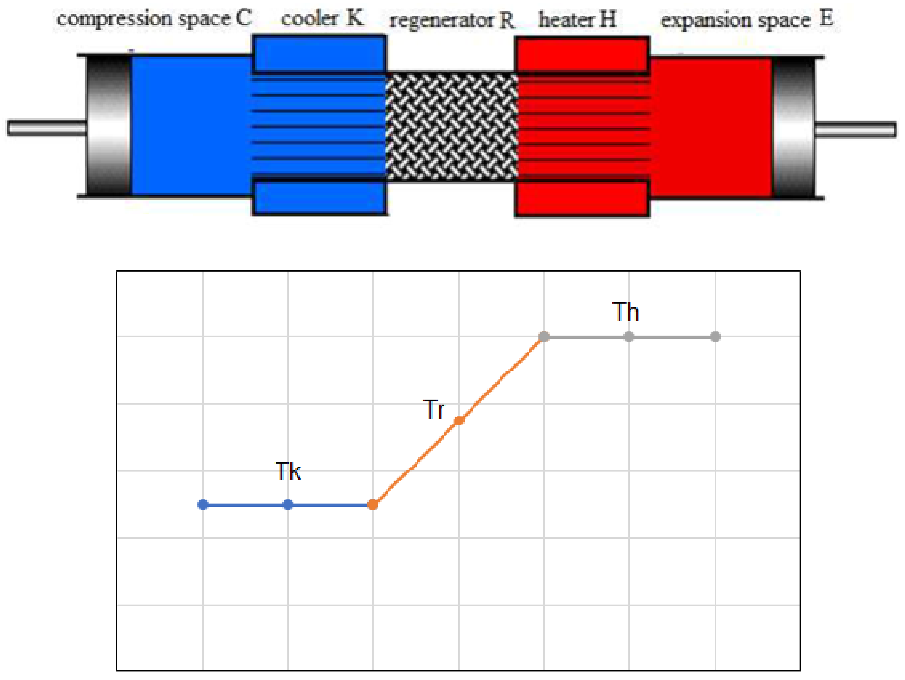
The second-order method is known as the “Schmidt analysis” and uses as simplification the isothermal transformation of both the expansion and the compression side. The temperature profile of the regenerator is constant as well and calculated as the logarithmic mean of the first two. The three sections of the engine are simplified as shown in Figure 12 [27,28].

This method is a simplified method as well and for an even more thorough analysis, the adiabatic model must be implemented. Therefore, discrepancies are expected between the calculated values with this method and the values measured experimentally.

Since the α-Stirling engine is a two-piston configuration, the model can be simplified using the equation presented by G. Walker in the 1980 “Stirling engines” manual [29], whose equation is presented as follows:

$$W=P·V_T·\frac{\left.\pi ·(1-AU\right)}{K+1}·{\left(\frac{1-DL}{1+DL}\right)}^{1/2}·\frac{\left.DL·sin(ET\right)}{1+{\left(1-D{L}^2\right)}^{1/2}}$$

(7)

The output of the equation, in this case, is the work per cycle of the Stirling cycle. This equation is also a function of three parameters:

$$S=\frac{2·RV·AU}{AU+1}$$

(8)

$$DL=\frac{{\left(A{U}^2+2·AU·K·cos\left(AL\right)+K^2\right)}^{1/2}}{\left(AU+K+2·S\right)}$$

(9)

$$ET=ta{n}^{-1}\left(\frac{\left.K·sin(AL\right)}{\left.AU+K·cos(AL\right)}\right)$$

(10)

These parameters have been calculated starting from the geometric and operative parameters of the engine. In

Table 7. Second-order analysis.

Definition	Symbol	U.O.M.	Value
Max pressure	P	Mpa	2.1
Total swept volume	VT	cm3	1049.2
Expansion swept volume	VL	cm3	657.94
Compression swept volume	VK	cm3	569.05
Swept volume ratio	K	-	1,16
Cold side temperature	TC	K	313
Hot side temperature	TH	K	1132
Temperature ratio	AU	-	0.28
Regenerator temperature	TR	K	637.09
Phase angle	AL	°	90
Total dead volume	VD	cm3	459.9
Dead volume ratio	RV	-	0.70
Work per cycle	W	J/cycle	372.98
Thermal power	Pth	W	3729.8
Cycle efficiency	%	-	30
Actual thermal power	Peff	W	1118.93

, the list of parameters and their respective values used for the calculation are reported. The results of such calculation can be highlighted in the bottom part of the table.

The result obtained through the Walker equation is comparable to the value obtained with the Beale equation. The two results are comparable: 1.18 kW for the Beale equation and 1.12 kW for the Walker equation.

As previously stated, these two methods provide estimated values of thermal output, but since the two values are very close, it is possible to confirm that the expected experimental values measured with this system will not have significant discrepancies with the calculated ones.

The cycle efficiency has been set at 30%. This value comes directly from Walker’s Stirling Engine Design Manual. In this work, the worst-case scenario presented by Walker has been evaluated and therefore the most pessimistic value.

This claim is supported by data found in literature which prove that efficiencies in Stirling engines range between high-20’s up to 42% [30].

By using these two methods, we can conclude that the value of thermal power that the system is able to produce in these conditions is 1.12 kW.

The last section of the analysis is the coupling of the system with a permanent magnet generator to verify the electrical output of the dish-Stirling. For a complete system, the Mecc Alte Eogen [31] generator can be coupled for the generation of electrical energy. The efficiency of generation for the chosen generator is 88%. In conclusion, the result of the entire analysis is presented in

Table 8. Results of the simulation.

Parameter	U.O.M.	Value
Average irradiance on the concentrator	W/m2	800
Hot side temperature reached	°C	859
Generated thermal power	kW	1.12
Efficiency of the electrical generator	%	88
Generated electrical power	kW	0.99

.

As shown in Table 8, an irradiance value of 800 W/m² allows the system to produce 996 W of electrical power.

The result of the simulation shows that a single-cylinder configuration of the engine with AISI 310 as coating material can allow the heat carrier fluid to reach a temperature of 859 °C.

This value can be used for the thermal energy production analysis, with an approximate resulting thermal power produced of 1.12 kW. Being the efficiency of the permanent magnet generator for this specific case equal to 88%, the resulting production of electrical energy is equal to 996 W. The result is in line with the expected results gained from the literature [32,33].

Furthermore, the specifics of the Genoastirling ML1000 single-cylinder Stirling engine set the maximum electrical power produced by the engine at 1.1 kW. This experimental value is close to the result obtained under similar conditions [34]. Therefore, it is possible to surmise that the electrical power produced by this technology, taking into consideration all the losses caused by the many components present in the system, is around 1 kW for a solar parabolic concentrator with a diameter of 2.4 m.

This result was compared with a much bigger CSP system with a production of 25 kW of electrical power simulated in similar conditions [35]. Obviously, since the diameter of the concentrator taken as comparison is much bigger (12.5 m² of diameter), the value taken for comparison is the power to area ratio to verify the effectiveness of the simulation. The modularity of the CSP technology should allow to obtain similar data from different sizes of concentrators.

In fact, the comparison from the simulation from literature allows to obtain a power-to-surface ratio equal to 0.204 kW/m². The current study simulated from Politecnico di Torino instead enables to reach a power-to-surface ratio equal to 0.205 kW/m². The results based on G. Walker’s analysis [29] showed that a CSP system is useful for micro-generation purposes. The simulation is in line with both data from similar size concentrators and with scaled concentrators with bigger sizes.

Table 9. Actual efficiency of the Stirling engine installed in the selected cities.

City	January	February	March	April	May	June	July	August	September	October	November	December
Teheran	0.29	0.32	0.33	0.34	0.34	0.34	0.34	0.33	0.32	0.31	0.28	0.27
Tabriz	0.28	0.32	0.33	0.34	0.34	0.34	0.34	0.33	0.32	0.3	0.28	0.26
Bandar Abbas	0.31	0.33	0.34	0.34	0.34	0.34	0.34	0.34	0.33	0.32	0.3	0.3
Rasht	0.28	0.31	0.33	0.34	0.34	0.34	0.34	0.33	0.32	0.3	0.27	0.26
Yazd	0.3	0.33	0.34	0.34	0.34	0.34	0.34	0.34	0.33	0.32	0.3	0.29

[36] compares the real efficiency of the Stirling engine mounted in various cities. This shows that the efficiency of the engine for small-scale microgeneration applications is stable between the high 20′s and 40%, with fluctuations during the different months of the year. The solar irradiance has also been compared to the same microgeneration systems to verify the validity of the simulation. Figure 13 shows irradiance values, which are coherent with the value recorded from this article.

5. Conclusions

The obtained result is interesting since the solar concentrator used for the project has a relatively small size. Therefore, by increasing the size of the concentrator, it is foreseeable to increase the energy production. However, the downside of this technology is represented by two main factors: the installation cost of such technologies, and the inconsistency of the mean solar irradiance. The latter can be analyzed in further detail by operating the previous simulations with a starting irradiance value of 400 W/m². The resulting electrical power output will drop to 810 W. This value was obtained by following the same steps of the analysis, starting from the temperature of the fluid in the internal pipe followed by the Stirling cycle analysis to produce electrical energy.

The drop in power output is not excessive but has to be taken into consideration for a potential productivity analysis on an annual basis. This is a disadvantage of any solar technology, which depends on the position of the Sun and its irradiance. However, the sun tracker placed on the concentrator enables to minimize these losses by following the movement of the Sun across the sky, compared to fixed systems such as photovoltaic panels for the small-scale generation which are not mounted with a tracking system and are therefore more subjected to these fluctuations.

The results show that this technology has various positive aspects, but also showed a margin of improvement to reach a clear and sustainable expansion which can eventually facilitate the highly required transition to “clean” energy production methods.

References

- Shahbaz, M.; Raghutla, C.; Chittedi, K.R.; Jiao, Z.; Vo, X.V. The effect of renewable energy consumption on economic growth: Evidence from the renewable energy country attractive index. Energy 2020, 207, 118162. [Google Scholar] [CrossRef]
- Lohani, B.; Tulej, P.; Dixon, R.K.; Frankl, P.; Amin, A.Z.; Alers, M.; Radka, M.; Monga, P.; George, A.M.; Giner-Reichl, I.; et al. An Agreement for the Establishment of the Caribbean Commission; International Organisations; University of Wisconsin Press: Madison, WI, USA, 1947; Volume 1, pp. 251–256. [Google Scholar]
- Devabhaktuni, V.; Alam, M.; Shekara Sreenadh Reddy Depuru, S.; Green, R.C.; Nims, D.; Near, C. Solar energy: Trends and enabling technologies. Renew. Sustain. Energy Rev. 2013, 19, 555–564. [Google Scholar] [CrossRef]
- Kabir, E.; Kumar, P.; Kumar, S.; Adelodun, A.A.; Kim, K.-H. Solar energy: Potential and future prospects. Renew. Sustain. Energy Rev. 2018, 82, 894–900. [Google Scholar] [CrossRef]
- Giovannelli, A. State of the Art on Small-Scale Concentrated Solar Power Plants. Energy Procedia 2015, 82, 607–614. [Google Scholar] [CrossRef] [Green Version]
- Ahmed, F.E.; Hashaikeh, R.; Hilal, N. Solar powered desalination–Technology, energy and future outlook. Desalination 2019, 453, 54–76. [Google Scholar] [CrossRef] [Green Version]
- Carrillo Caballero, G.E.; Mendoza, L.S.; Martinez, A.M.; Silva, E.E.; Melian, V.R.; Venturini, O.J.; del Olmo, O.A. Optimization of a Dish Stirling system working with DIR-type receiver using multi-objective techniques. Appl. Energy 2017, 204, 271–286. [Google Scholar] [CrossRef]
- Roth, P.; Georgiev, A.; Boudinov, H. Cheap two axis sun following device. Energy Convers. Manag. 2005, 46, 1179–1192. [Google Scholar] [CrossRef]
- Siva Reddy, V.; Kaushik, S.C.; Ranjan, K.R.; Tyagi, S.K. State-of-the-art of solar thermal power plants—A review. Renew. Sustain. Energy Rev. 2013, 27, 258–273. [Google Scholar] [CrossRef]
- Sobri, S.; Koohi-Kamali, S.; Rahim, N.A. Solar photovoltaic generation forecasting methods: A review. Energy Convers. Manag. 2018, 156, 459–497. [Google Scholar] [CrossRef]
- Islam, M.T.; Huda, N.; Abdullah, A.B.; Saidur, R. A comprehensive review of state-of-the-art concentrating solar power (CSP) technologies: Current status and research trends. Renew. Sustain. Energy Rev. 2018, 91, 987–1018. [Google Scholar] [CrossRef]
- Ummadisingu, A.; Soni, M.S. Concentrating solar power–Technology, potential and policy in India. Renew. Sustain. Energy Rev. 2011, 15, 5169–5175. [Google Scholar] [CrossRef]
- Braun, F.G.; Hooper, E.; Wand, R.; Zloczysti, P. Holding a candle to innovation in concentrating solar power technologies: A study drawing on patent data. Energy Policy 2011, 39, 2441–2456. [Google Scholar] [CrossRef]
- Suresh, N.S.; Thirumalai, N.C.; Rao, B.S.; Ramaswamy, M.A. Methodology for sizing the solar field for parabolic trough technology with thermal storage and hybridization. Sol. Energy 2014, 110, 247–259. [Google Scholar] [CrossRef] [Green Version]
- Solana Solar Power Generating Station, Arizona, US-Power Technology|Energy News and Market Analysis. Available online: https://www.power-technology.com/projects/solana-solar-power-generating-arizona-us/ (accessed on 24 June 2021).
- Coco-Enríquez, L.; Muñoz-Antón, J.; Martínez-Val, J.M. Integration between direct steam generation in linear solar collectors and supercritical carbon dioxide Brayton power cycles. Int. J. Hydrog. Energy 2015, 40, 15284–15300. [Google Scholar] [CrossRef] [Green Version]
- Elsafi, A.M. On thermo-hydraulic modeling of direct steam generation. Sol. Energy 2015, 120, 636–650. [Google Scholar] [CrossRef]
- Mancini, T.; Heller, P.; Butler, B.; Osborn, B.; Schiel, W.; Goldberg, V.; Buck, R.; Diver, R.; Andraka, C.; Moreno, J. Dish-Stirling Systems: An Overview of Development and Status. J. Sol. Energy Eng. 2003, 125, 135–151. [Google Scholar] [CrossRef]
- Barlev, D.; Vidu, R.; Stroeve, P. Innovation in concentrated solar power. Sol. Energy Mater. Sol. Cells 2011, 95, 2703–2725. [Google Scholar] [CrossRef]
- Zayed, M.E.; Zhao, J.; Elsheikh, A.H.; Zhao, Z.; Zhong, S.; Kabeel, A.E. Comprehensive parametric analysis, design and performance assessment of a solar dish/Stirling system. Process. Saf. Environ. Prot. 2021, 146, 276–291. [Google Scholar] [CrossRef]
- Romage, G.; Jiménez, C.; de Jesús Reyes, J.; Zacarías, A.; Carvajal, I.; Jiménez, J.A.; Pineda, J.; Venegas, M. Modeling and Simulation of a Hybrid Compression/Absorption Chiller Driven by Stirling Engine and Solar Dish Collector. Appl. Sci. 2020, 10, 9018. [Google Scholar] [CrossRef]
- Nielsen, A.S.; York, B.T.; MacDonald, B.D. Stirling engine regenerators: How to attain over 95% regenerator effectiveness with sub-regenerators and thermal mass ratios. Appl. Energy 2019, 253, 113557. [Google Scholar] [CrossRef]
- Barreto, G.; Canhoto, P. Modelling of a Stirling engine with parabolic dish for thermal to electric conversion of solar energy. Energy Convers. Manag. 2017, 132, 119–135. [Google Scholar] [CrossRef]
- Thombare, D.G.; Verma, S.K. Technological development in the Stirling cycle engines. Renew. Sustain. Energy Rev. 2008, 12, 1–38. [Google Scholar] [CrossRef]
- Torres García, M.; Carvajal Trujillo, E.; Vélez Godiño, J.; Sánchez Martínez, D. Thermodynamic Model for Performance Analysis of a Stirling Engine Prototype. Energies 2018, 11, 2655. [Google Scholar] [CrossRef] [Green Version]
- Hirve, N.S. Thermodynamic Analysis of a Stirling Engine Using Second Order Isothermal and Adiabatic Models for Application in Micropower Generation System. Master’s Thesis, University of Washington, Seattle, WA, USA, 2015. [Google Scholar]
- Organ, A.J. Thermodynamic Analysis of the Stirling Cycle Machine—A Review of the Literature. Proc. Inst. Mech. Eng. Part. C J. Mech. Eng. Sci. 1987, 201, 381–402. [Google Scholar] [CrossRef]
- Urieli, I.; Berchowitz, D.M. Stirling Cycle Engine Analysis; Adam Hilger Ltd.: London, UK, 1984. [Google Scholar]
- Walker, G. Stirling Engines; Clarendon Press: Oxford, UK, 1980; ISBN 978-0-19-856209-2. [Google Scholar]
- Zayed, M.E.; Zhao, J.; Elsheikh, A.H.; Li, W.; Sadek, S.; Aboelmaaref, M.M. A comprehensive review on Dish/Stirling concentrated solar power systems: Design, optical and geometrical analyses, thermal performance assessment, and applications. J. Clean. Prod. 2021, 283, 124664. [Google Scholar] [CrossRef]
- Magneti Permanenti|Mecc Alte. Available online: https://www.meccalte.com/it/prodotti/alternatori/magneti-permanenti (accessed on 24 June 2021).
- Zhang, C.; Xu, Q.; Zhang, Y.; Arauzo, I.; Zou, C. Performance analysis of different arrangements of a new layout dish-Stirling system. Energy Rep. 2021, 7, 1798–1807. [Google Scholar] [CrossRef]
- Hafez, A.Z.; Soliman, A.; El-Metwally, K.A.; Ismail, I.M. Solar parabolic dish Stirling engine system design, simulation, and thermal analysis. Energy Convers. Manag. 2016, 126, 60–75. [Google Scholar] [CrossRef]
- Motore ML1000|I Nostri Motori|Genoastirling. Available online: https://genoastirling.it/ita/motore-ml1000.php (accessed on 24 June 2021).
- Lashari, A.A.; Shaikh, P.H.; Leghari, Z.H.; Soomro, M.I.; Memon, Z.A.; Uqaili, M.A. The performance prediction and techno-economic analyses of a stand-alone parabolic solar dish/stirling system, for Jamshoro, Pakistan. Clean. Eng. Technol. 2021, 2, 100064. [Google Scholar]
- Moghadam, R.S.; Sayyaadi, H.; Hosseinzade, H. Sizing a solar dish Stirling micro-CHP system for residential application in diverse climatic conditions based on 3E analysis. Energy Convers. Manag. 2013, 75, 348–365. [Google Scholar] [CrossRef]
Figure 1.
Global investment in renewable energies in billion dollars: period 2004–2014 [2].
Figure 2.
Solar power technologies.
Figure 3.
EuroDISH system, Almería.
Figure 4.
Geometry of a parabolic concentrator.
Figure 5.
Genoastirling engines.
Figure 6.
Hot side heat exchanger.
Figure 7.
Configurations for the CFD simulation.
Figure 8.
(a) Single-cylinder temperature profile (in K). (b) Twin-cylinder temperature profile (in K).
Figure 9.
Geometry of the exchanger tube.
Figure 10.
Temperature profiles in the internal tube. (A) AISI 310, (B) Inconel 625.
Figure 11.
Hot air temperature profile. (A) k-ε, (B) k-Ω.
Figure 12.
Temperature profile of the engine.
Figure 13.
Monthly solar irradiance in the selected cities.