A Real-Time Optimization Strategy for Small-Scale Facilities and Implementation in a Gas Processing Unit

Abstract

The rise of new digital technologies and their applications in several areas pushes the process industry to update its methodologies with more intensive use of mathematical models—commonly denoted as digital twins—and artificial intelligence (AI) approaches to continuously enhance operational efficiency. In this context, Real-time Optimization (RTO) is a strategy that is able to maximize an economic function while respecting the existing constraints, which enables keeping the operation at its optimum point even though the plant is subjected to nonlinear behavior and frequent disturbances. However, the investment related to the project of commercial RTOs may make its application infeasible for small-scale facilities. In this work, an in-house, small-scale RTO is presented and its successful application in a real industrial case—a Natural Gas Processing Unit—is shown. Besides that, a new method for enhancing the efficiency of using sequential-modular simulator inside an optimization framework and a new method to account for the economic return of optimization-based tools are proposed and described. The application of RTO in the industrial case showed an enhancement in the stability of the main variables and an increase in profit of 0.64% when compared to the operation of the regulatory control layer alone.

1. Introduction

Real-time optimization is a model-based adaptive optimization technique that attempts to find the optimal operating condition accordingly to an economic index of a plant subjected to a process model and a set of constraints that might be, for instance, physical limits, environmental restriction, product quality, or safety criteria [1]. The so-called “two-step” approach proposed by Jang et al. [2] has become the most widespread RTO strategies in industry [3,4,5]. In this approach, a parameter estimation step is performed followed by an economic optimization step, so that the available static model of the plant can be adjusted considering the most recent set of plant information and the optimization may be carried out considering a rigorous model with minimum plant-model mismatch. It is true that this approach may fail when there is model structural uncertainty [6,7]. However, when the sources of uncertainty are mainly parametric, the approach has great potential to increase the economic performance of process operations [8] and to provide considerable economic benefit that overly surpass the cost of investment on the RTO design. Therefore, the development of a rigorous process model is the backbone of the two-step RTO approach and, in fact, it is possible to show that whenever a model satisfies the set of model adequacy criteria, the model-based optimization problem is able to drive the plant to its true optimum [9,10,11].

In the classical scheme of the two-step RTO, a parameter estimation subjected to the same static model used in the optimization step is carried out once the input data is guaranteed to be in a stationary state. To cope with this requirement, a steady-state detection (SSD) method is implemented. There are several SSD methods available, most of them are statistical-based methods, such as the F-test [12] and the Student’s t-test [13,14]. Recently, two research groups have proposed removing the SSD requirement by proceeding a dynamic estimation, such as the Extended Kalman Filter, in a framework called Hybrid RTO (HRTO) [15,16]. Although this method presents a high potential to speed up RTO cycles and to reduce the suboptimal operation time, it lacks industrial validation.

Recently, the academic literature of RTO has been focused on solving the problem of finding the true-plant optimum in cases related to serious structural plant-model mismatch. Since the proposition of the Integrated System Optimization and Parameter Estimation (ISOPE) algorithm by Roberts [17], which led to the Constraint Adaption (CA) [18] and the Modifier Adaption (MA) [19] algorithms, several derivations have been proposed so far to cope with different methodological paths, a detailed review on MA approaches and applications can be found in Marchetti et al. [7]. These approaches are based on the introduction of zeroth-and first-order modifiers to adapt the model-based optimization problem. The modifiers are calculated from plant measurements and estimation of the plant gradients in relation to the decision variables. In the CA algorithm, the modifiers are used to adapt the constraints of the problem, so that the model-based constraints meet the plant constraints upon convergence. In the MA algorithm, both the constraints and objective function are adapted, so that the model-based optimization problem matches the optimality condition of the plant upon convergence. However, the requirement of estimating the plant gradients in the absence of a reliable model is one of the main reasons that justify the low number of industrial applications of MA approaches. Recently, an industrial application of CA in a solid-oxide fuel-cell system has been disclosed [20,21], but the problem was formulated in a manner such that the first-order modifiers were not necessary because the plant optimum was known to be located at the intersection of active constraints, so the gradient estimation was not required. In spite of that, the work was a proof of concept and may indicate the increase of initiatives of MA in the industry, especially with the rise of new methodologies that merge concepts of Machine Learning and RTO to produce better estimates of the first-order modifiers, such as the MA with Quadratic Approximation (MAWQA) [22,23], the use of neural networks [24], Gaussian process [25,26], and Bayesian optimization [27].

In the process industry, RTO is typically implemented as the two-step approach and in a hierarchical control pyramid manner [28]. In a simplified and summarized description, the regulatory control layer is implemented to deal with high-frequency disturbances of the process, typically in a multiloop PID controllers approach. This layer is able to interact with the plant in the scale of seconds, rejecting fast disturbances and keeping the stability of the operation. In the upper layer, the supervisory control layer, a model-based approach is used to determine the optimal trajectories of the process by the use of simple dynamic models, typically linear ones, with the objective to track setpoints and send control actions as setpoints to the regulatory layer. This layer works in the time scale of minutes and the most-used technique is model predictive control (MPC). The optimization layer comes above the previous control layers in order to determine the economic optimal operating point of the process. This layer typically runs in the time scale of hour due to the complexity of the models that are used.

In the context of modeling strategies, there are mainly two types of simulators available for developing the process flow-sheets, they are the so-called Equation-Oriented (EO) simulators and Sequential-Modular (SM) simulators. 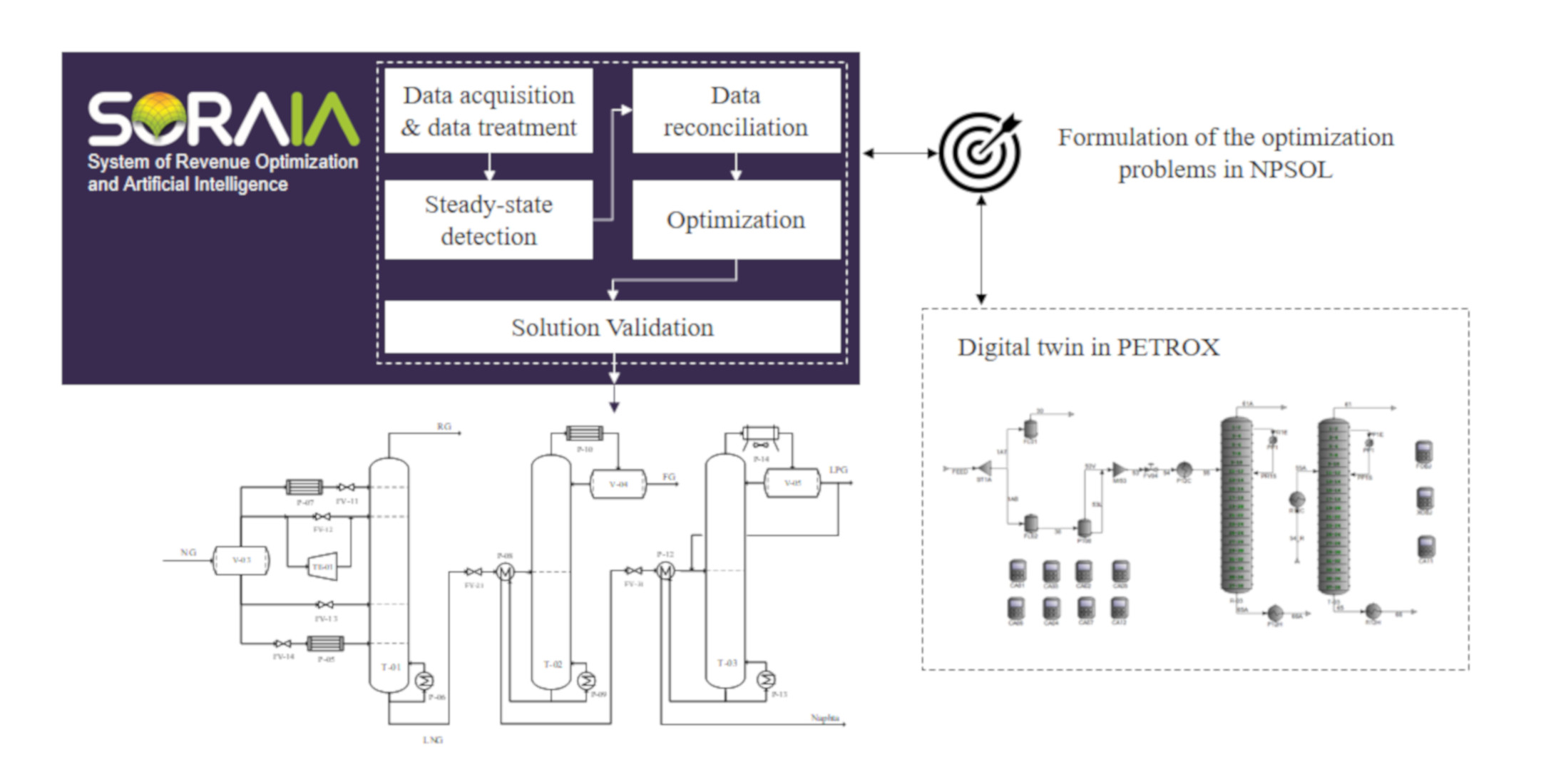Despite the undoubted advantages of using EO simulators [29] and the vast quantities academic works using and developing methodologies based on them, the availability of SM models in industry is still high due to their ability to solve a problem with low initialization effort and an easier flow-sheet design [30]. However, the computational cost to handle nested recycles can hinder their use in the context of real-time optimization. Early works proposed the use of a method called the Modular Continuous (MC) approach [31], or infeasible path [32,33], in which the convergence loops are removed from the SM simulator and convergence of the model is assured by a higher-level optimization layer. Recent works have proposed the use of surrogate models to enhance reliability and reduce the computational effort of the optimization [34,35]. The present work proposes an extension of the concept of the MC approach, by adding an acceleration step of successive substitution in the model flow-sheet.

Despite significant advances in the field of controller performance assessment since the 1960s, these advances have been focused on univariable control structures and on obtaining a technical metric [36]. In fact, there has been very little discussion regarding the economic assessment of advanced process control and optimization applications [37]. There are many works that disclose the economic return of RTO’s application [38], but it is not clear whether these numbers are trustworthy or not since the authors do not discuss their methods of assessing this economic benefit. Beyond the standard discount cash flow analysis [39], which can be used both to support decision-making at the investment stage and to perform economic assessment in an existing application, three methodologies are worth mentioning: the performance assessment of MPC proposed by Xu et al. [40]; the framework proposed by Bauer and Craig [37]; and the systematic method proposed by Udugama et al. [36]. However, the three methods have the similarity of not considering an optimization layer in their assumptions. They can account for the benefit of reducing the process variability and the distance from the desired setpoints, however, they do not account for true optimal operation. Therefore, reliable methods to assess the economic benefit of advanced control structures and RTO frameworks are still an open issue.

Petrobras started investing in RTO technology in 2004. Their early developments were based on commercial tools, such as Aspen Plus (AspenTech) and Romeo (Aveva), but using self-developed models. 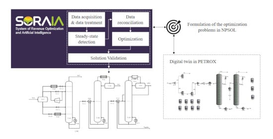Since then, the company has achieved great expertise in the technology and successful applications have been reported in Gas Processing Units [41], Fluidized Catalytic Cracker Units [42], and Crude Distillation Units [29]. However, applications with small-scale scopes may not benefit from the application of these tools since the economic return may be smaller than the cost of investment in the project stage, annual licensing of the software, and often the need for external consultancy during the operation phase. Therefore, Petrobras and LADES, the Software Development Laboratory (LADES) of COPPE/UFRJ, collaborated to develop an in-house RTO software, which was called SoraIA, an acronym in Portuguese for ”System of Revenue Optimization and Artificial Intelligence“. The software presented some advantages due to the fact of being totally based on open-source or acquired tools, having ease of maintenance and also adaptability for applications in new processing units, allied with high flexibility for different problem formulations and small investment requirements compared with the great economic return.

Besides the description of the developed software and its application in a real industrial facility, this paper also discloses two contributions to the RTO literature in the sense of process modeling with the proposed “Modular Continuous with Successive Substitution” and a new method to assess RTO’s economic return after its implementation, as well as its potential further economic benefit that would be possible with system improvement.

The software was tested in an industrial Gas Processing facility owned by Petrobras. RTO was implemented in a closed loop with the control system of the unit, and the results and discussion are provided in this paper. Further, after three months of operation, the economic return of the system was evaluated accordingly with the new proposed method and the result overcame the initial expectations of the project, even though the unit is highly instrumented and very well operated in the open loop—that is, considering only the regulatory control under the supervision of the operation team, without the action of any advanced control strategy.

The present paper is organized as follows: Section 2 presents the methodology proposed in this paper in a generalized manner; Section 3 presents how the methodology was applied to the industrial case that is object of the present application; Section 4 presents the results and discussion of the present application regarding the reconciliation problem, the optimization problem, the computational cost, and the economic benefit of RTO; finally, Section 5 presents the conclusion of the present work.

2. Methodology

2.1. Modular Continuous with Successive Substitution

The quality of the model used in the two-step RTO is crucial for the success of the application—that is, the model should be simple enough so its computational cost can be suitable for optimization purposes and detailed enough to mitigate any serious structural uncertainty, since the approach is only able to deal with parametric uncertainty. Although it is difficult to measure, Forbes and Marlin [43] developed a criteria to determine whether a model is adequate to be used in the two-step approach based on its capability to match the Karush–Kuhn–Tucker (KKT) optimality conditions [44] of the plant at the optimal point.

The EO and SM strategies have their benefits and drawbacks for the application in an RTO framework. For example, SM has dedicated numerical methods to converge each process unit, which makes this approach more robust for poor initial estimates. However, this type of model can be very costly to run, demanding several loops of convergence, which frequently make them unsuitable for optimization purposes. On the other hand, EO models are fast and efficient to be evaluated, they also present the advantage of providing accurate gradient estimates from automatic differentiation strategies. However, this type of modeling is highly dependent on the initial estimates of the dependent variables, since its convergence algorithms provide the solution of the full system of equations simultaneously. Therefore, a common choice is to use both approaches together, running the SM model first to provide better initial estimates for the EO model that is used inside the optimization framework. However, this common choice comes with the cost of having to develop two compatible models, frequently in different platforms.

In this work, a modeling approach was developed to handle an SM model inside the optimization framework in an efficient manner. The idea is derived from the early proposition by Berna et al. [31] and Biegler and Hughes [45] in the Modular Continuous (MC) approach, where the main idea consists on opening mass and energy loops and transforming them into new decision variables and constraints to be met by the optimization problem. As the model would not be converged along the optimization steps, this approach was also known as infeasible path, due to the fact that the model convergence is only assured upon optimization convergence [32,33]. Here, the proposed approach, “Modular Continuous with Successive Substitution” (MCSS), follows the same philosophy proposed by the early works of the MC approach.

Figure 1 illustrates the algorithmic procedures that are performed for any module i inside loops in order to carry out the optimization based on the SM, MC, and the proposed MCSS approaches, in which $\mathit{u}\in {\mathbb{R}}^{n_u}=\mathbb{U}$ is the set of all input variables, $\mathit{y}\in {\mathbb{R}}^{n_y}=\mathbb{Y}$ represents the set of all output variables of the model, $\mathit{z}\in \mathit{y}$ is a subset of the output variables that represents the material and energy loop streams of the model, and $\mathbf{\rho }\in {\mathbb{R}}^{n_{\rho }}=\mathbb{P}$ is the set of independent variables introduced by the opened loops.

Following the nomenclature introduced in Figure 1, the i loops represented by variable $z_i$ in Figure 1a are torn into two variables ${\rho }_i$ and $z_i^{ref}$ in Figure 1c. In the MCSS approach, all modules inside the opened loops are replicated into the reference modules: variables ${\rho }_i$ are the degrees of freedom of the optimizer and $z_i^{ref}$ are the loop output variables of the reference module. $z_i^{ref}$ is returned as input for the second module. In this way, a first step of successive substitution is forced within the process model. The convergence is guaranteed by the addition of constraints that enforce that all loops are closed upon convergence. In the MC approach, this set of constraints are

$$\mathbf{\rho }-\mathit{z}=0,$$

(1)

while, in the proposed MCSS, the set of constraints are

$$\mathit{z}-{\mathit{z}}^{ref}=0.$$

(2)

The main goal of the MC approach is to reduce the number of convergence loops in the simulation layer by transferring the convergence conditions of the model to the higher-level optimization layer. The purpose of the additional successive substitution step in the MCSS approach is to accelerate the convergence by approximating the feasible path characteristic of the SM approach, but still keeping the faster convergence provided by the infeasible path of the MC approach.

PETROX, the simulator used in this work, is a reliable SM simulator developed for giving support to process design at Petrobras [46]. The success of this software can be addressed for the vast library of process units and the reliability of its internal numerical methods. Nowadays, the software is also applied to develop reliable digital twins of the different units of the company. This work opened a new perspective for its application in optimization by following the philosophy of the Modular Continuous with Successive Substitution. Some rules of thumb of the modeling approach used in the present work are summarized in the following:

• Parameterization of the feed composition—with the composition of the product streams as specification, the feed composition can be constructed by setting some criteria, such as meeting dew or boiling temperatures in flash units and meeting components ratio with the product.
• Simplification of process units that are not essential for the optimization scope—distillation columns before the actual scope of the optimization can be replaced by a simple approach based on flashes with parameterized fractioning ratio between cut components;
• Avoid loops for mass and energy integration—opening loops and forcing a first successive substitution;
• No additional convergence loops—remove any controller loops to meet specification criteria, this task should be passed to the parameter-estimation layer.

In this work, the model developed in PETROX is denoted as a stationary map of the inputs and parameters into the outputs:

$$\mathit{y}=\mathcal{F}(\mathbf{\rho },\mathbf{\theta },\mathit{u}),$$

(3)

where $\mathbf{\theta }\in {\mathbb{R}}^{n_{\theta }}=\mathbb{T}$ is the set of adjustable parameters. For the sake of simplifying notation, and without loss of generality, the static mapping will be frequently denoted only by $\mathit{y}(\mathbf{\rho },\mathbf{\theta },\mathit{u})$. Additionally, all objective functions and nonlinear constraints are also provided by the SM simulator.

2.2. RTO Architecture

An in-house software was developed with the purpose of performing all RTO stages. Apart for some specific details, the presented structure is very similar to what has been done since the 1980s in the two-step RTO, the main contribution of this work is the use of the MCSS approach, as it is described in the formulation of the optimization problems in Section 2.2.4 and Section 2.2.5. Figure 2 illustrates the architecture of the SoraIA software.

The main core was written in C++ and its purpose is to manage the information flow in order to perform the desired tasks that are required by RTO methodology. Six main routines are executed in sequence: data acquisition, data treatment, steady-state detection, data reconciliation, optimization, and solution validation. The software is able to communicate with the process database and the solution database, and perform the interface between the process simulator (PETROX) and the nonlinear optimization solver (NPSOL). In addition, the user can configure some features of the run by a web interface. This interface compiles the set of user configurations into some standard text files that can be read by the C++ core in order to shape each routine accordingly.

Every run cycle of RTO starts with the data acquisition routine and follows the routine’s sequence until the optimal solution is obtained, except in the case where some major problem is found during any stage of the run. In this case, the software is aborted and a new cycle is started. In the following, each of the main RTO routines are further described.

2.2.1. Data Acquisition

In the data acquisition stage, the user can specify whether the software is going to run offline, so a specific operational point can run for tests independently of the actual state of the plant, or whether the software is going to run online, reading the values directly from the process database. In this stage, the user can define the size of the acquired data window and which instrument tags are related to which input variables from the process model simulator.

2.2.2. Data Treatment

In the data treatment stage, each input variable is treated by a linear transformation specified by the user in order to scale or to perform any required unit change. In addition, there are some verifications in the read information in order to exclude any unwanted null values, strings, or unexpected out-of-limit values. If any abnormal value is found in this verification, the software is restarted, so its cycle is repeated until there is no error in the input values.

2.2.3. Steady-State Detection

It is very important to assure that the data used in the data reconciliation stage is in stationary state in order to reliably estimate the model parameters. Therefore, the steady-state detection is mandatory and whenever it is detected that the read data window presents some dynamics, its cycle is restarted until the steady-state is detected in the input data window. There are several steady-state detection (SSD) techniques, Cao and Rhinehart [47] briefly reviewed some of the existing methods and proposed an efficient new statistical method. Later, Bhat and Saraf [12] also outlined aspects of the available SSD techniques and extended the proposition of Cao and Rhinehart [47].

In this work, two statistical tests were applied. The first test is based on cutting the input window in three periods and comparing these windows to each other in order to check whether their means are equivalent by a Student’s t-test. The second is an analysis where the variance of the variables are verified within some desirable limits. These limits are estimated using past historical data by selecting periods where the variables were in the steady-state condition. Both tests are well-established in the literature [12]. However, the combination of these methods are a contribution of the present work, to the best of the authors’ knowledge. This proposition is made in order to overcome the limitation of the t-test when too-high variance values are observed, in which false detections are observed. Therefore, the stationary condition must be detected in both tests so the data window is allowed to go to the next stage; otherwise, a new RTO cycle starts.

2.2.4. Data Reconciliation and Parameter Estimation

The data reconciliation problem was formulated in a manner that it can perform a simultaneous parameter estimation, as proposed by Rod and HanČl [48]. Differently from the usual approach in the literature, not only the adjustable parameters of the process unit models are estimated, but also the parameters that were added to ensure convergence of the model, following the one-pass modeling philosophy described in Section 2.1. The data reconciliation problem is formulated as a nonlinear programming problem:

$$\begin{array}{cc}\hfill {\overline{\mathbf{\rho }}}_k,{\overline{\mathbf{\theta }}}_k,{\overline{\mathit{u}}}_k^{rdf}=\arg \underset{\mathbf{\rho },\mathbf{\theta },{\mathit{u}}^{rdf}}{\min }& {\mathcal{J}}_{rec}({\mathit{y}}^{rec},{\mathit{y}}_k^m,{\mathit{u}}^{rec},{\mathit{u}}_k^m)\hfill \end{array}$$

(4a)

$$\begin{array}{cc}\hfill \mathrm{s}.\mathrm{t}.& \mathit{y}=\mathcal{F}(\mathbf{\rho },\mathbf{\theta },\mathit{u})\hfill \end{array}$$

(4b)

$$\begin{array}{cc}\hfill & \mathcal{G}(\mathbf{\rho },\mathbf{\theta },\mathit{u})\le \mathbf{0}\hfill \end{array}$$

(4c)

$$\begin{array}{cc}\hfill & \mathit{z}-{\mathit{z}}^{ref}=0\hfill \end{array}$$

(4d)

$$\begin{array}{cc}\hfill & {\mathbf{\theta }}_{lb}\le \mathbf{\theta }\le {\mathbf{\theta }}_{ub}\hfill \end{array}$$

(4e)

$$\begin{array}{cc}\hfill & {\mathit{u}}_{lb}^{rdf}\le {\mathit{u}}^{rdf}\le {\mathit{u}}_{ub}^{rdf},\hfill \end{array}$$

(4f)

where $\mathbf{\rho }\in \mathbb{P}$ is the set of additional decision variables added by the MCSS approach; $\mathbf{\theta }\in \mathbb{T}$ is the set of all adjustable parameters to be estimated; the superscripts ${(·)}^{rdf}$ mean “reconciliation degree of freedom”, so ${\mathit{u}}^{rdf}\subset \mathbb{U}$ is the set of $n_u^{rdf}$ uncertain inputs that are considered degrees of freedom in the reconciliation problem; ${\mathit{u}}^{rec}\subset {\mathit{u}}^{rdf}$ is the set of $n_{u_r}$ reconciled inputs, which is a subset of the uncertain inputs that have available measurements; $\mathit{u}\in {\mathbb{R}}^{n_u}$ is the set of all input variables; and ${\mathit{y}}^{rec}\subset \mathit{y}$ is the set of $n_{y_r}$ reconciled output variables, which is a subset of the output variables that have available measurements. The vectors ${\mathit{u}}^m\in {\mathbb{R}}^{n_u^m}$ and ${\mathit{y}}^m\in {\mathbb{R}}^{n_y^m}$ are the measurements of the input and output variables, respectively. The function $\mathcal{G}:{\mathbb{R}}^{n_{\theta }}\times {\mathbb{R}}^{n_u}\to {\mathbb{R}}^{n_g}$ is the set of static mappings of the parameters and inputs into the nonlinear constraints, and the objective function ${\mathcal{J}}_{rec}:{\mathbb{R}}^{n_y^m}\times {\mathbb{R}}^{n_y^m}\times {\mathbb{R}}^{n_u^m}\times {\mathbb{R}}^{n_u^m}\to \mathbb{R}$ is the weighted sum of squared errors between predicted and measured variables. $\mathit{z}$ and ${\mathit{z}}^{ref}$ are the output of the actual and the reference modules of the opened loops added for the MCSS approach. Finally, the subscript ${(·)}_k$ denotes the $k^{th}$ run of RTO, the bar emphasis $\left(\overline{·}\right)$ denotes the optimal values obtained in the run, and the subscripts ${(·)}_{lb}$ and ${(·)}_{ub}$ denote lower and upper bounds, respectively. It is noteworthy that the $k^{th}$ values inserted in the problem for the sets of input and output measurements, ${\mathit{u}}_k^m$ and ${\mathit{y}}_k^m$, are the arithmetic mean of the time window acquired in the data acquisition stage.

After running the reconciliation problem, it is possible to define the offsets of the output measurements, which are defined by the deviation between the measured and the predicted variable:

$${\mathbf{\epsilon }}_k^y={\mathit{y}}_k^m-\mathit{y}({\overline{\mathbf{\rho }}}_k,{\overline{\mathbf{\theta }}}_k,\mathit{u}\left({\overline{\mathit{u}}}_k\right))$$

(5)

and the offsets of the input variables, which are defined by the deviation between the measured input and the optimal input:

$${\mathbf{\epsilon }}_k^u={\mathit{u}}_k^m-{\overline{\mathit{u}}}_k^m.$$

(6)

2.2.5. Optimization Problem

In the optimization problem, as in the reconciliation problem, the objective function and constraints are evaluated by the process simulator and the main core of the software is responsible for managing the information flow between the simulator and the optimizer. The formulation of the optimization problem is presented below:

$$\begin{array}{cc}\hfill {\overline{\mathbf{\rho }}}_k,{\overline{\mathit{u}}}_k^{odf}=\arg \underset{\mathbf{\rho },{\mathit{u}}^{odf}}{\min }& {\mathcal{J}}_{opt}(\mathit{u},\mathit{y})\hfill \end{array}$$

(7a)

$$\begin{array}{cc}\hfill \mathrm{s}.\mathrm{t}.& \mathit{y}=\mathcal{F}(\mathbf{\rho },{\overline{\mathbf{\theta }}}_k,\mathit{u})\hfill \end{array}$$

(7b)

$$\begin{array}{cc}\hfill & \mathcal{G}(\mathbf{\rho },{\overline{\mathbf{\theta }}}_k,\mathit{u})\le \mathbf{0}\hfill \end{array}$$

(7c)

$$\begin{array}{cc}\hfill & \mathit{z}-{\mathit{z}}^{ref}=0\hfill \end{array}$$

(7d)

$$\begin{array}{cc}\hfill & {\mathit{y}}_{lb}-{\mathbf{\epsilon }}_k^y\le \mathit{y}\le {\mathit{y}}_{ub}-{\mathbf{\epsilon }}_k^y\hfill \end{array}$$

(7e)

$$\begin{array}{cc}\hfill & {\mathit{u}}_{lb}^{odf}-\mathit{H}{\mathbf{\epsilon }}_k^u\le {\mathit{u}}^{odf}\le {\mathit{u}}_{ub}^{odf}-\mathit{H}{\mathbf{\epsilon }}_k^u,\hfill \end{array}$$

(7f)

where the function ${\mathcal{J}}_{opt}:\mathbb{U}\times \mathbb{Y}\to \mathbb{R}$ is the economic objective function of the optimization problem; this function is usually an economic balance between the incomes with products and the costs with raw materials and energy consumption. The superscript ${(·)}^{odf}$ means “optimization degree of freedom”, so ${\mathit{u}}^{odf}\subset \mathbb{U}$ is the set of $n_u^{odf}$ inputs for which the objective function is sensible to variations within their feasible space, corresponding to the set of degrees of freedom of the optimization problem. It is important to highlight that all adjustable parameters and uncertain inputs—which are not degrees of freedom of the optimization—that were estimated in the data reconciliation problem are kept fixed in the optimization problem. In addition, the estimated offsets, ${\mathbf{\epsilon }}_k^y$ and ${\mathbf{\epsilon }}_k^u$, are used to shift the feasible space of the output variables, as in Equation (7e), and of the degrees of freedom for which there are available measurements, as in Equation (7f). Matrix $\mathit{H}\in {\{0;1\}}^{n_u^{odf}}\times {\{0;1\}}^{n_u^m}$ is a rectangular matrix of zeros and ones only to select which offset is related to which degree of freedom, considering that some degrees of freedom might not be related to any offset and the opposite can also be true.

2.2.6. Solution Validation

In the solution validation stage, there is an optimization flag check to verify whether the solution of the optimization problem was found within the constraints or whether it reached an infeasible solution, which is rarely expected to occur. If the solver returns an infeasible solution, the software will disregard this point and the RTO cycle will restart. On the contrary, the solution is shifted by the estimated offsets:

$${\mathit{y}}^{irv}=\mathit{y}({\overline{\mathbf{\rho }}}_k,{\overline{\mathbf{\theta }}}_k,\mathit{u}({\overline{\mathit{u}}}_k^{odf}))+{\mathbf{\epsilon }}_k^y,$$

(8)

$${\mathit{u}}^{irv}={\overline{\mathit{u}}}_k^{odf}+\mathit{H}{\mathbf{\epsilon }}_k^u,$$

(9)

where the superscript ${(·)}^{irv}$ means “ideal value at rest”; these values are written in the solution database. Once the new solution is written in the solution database, it is instantaneously available to be read by other instances of the control hierarchy.

2.2.7. Interface between PETROX and NPSOL Solver

The optimization solver used in the RTO is NPSOL version 5.0 [49]. This is a nonlinear programming solver written in Fortran 66 Version 2.1 that performs a Sequential Quadratic Programming (SQP) algorithm. The model was developed in PETROX 3.8 and its interface with the main core of RTO in C++ is carried out by PetroxTR 3.4R0. In order to improve the numerical robustness of the optimization, the decision variables, constraints, and objective function are normalized between the interval $(-1,1)$ according to a normalization space defined by the user. In addition, the version of the simulator PETROX used has no resource to provide information about the gradients of the objective function and the constraints with respect to the decision variables, since the simulator was not developed for optimization purposes. Therefore, the method used to estimate the gradient is based on finite difference approximations. For each decision variable, if the lower bound is active, a first-order forward finite difference is performed; if the upper bound is active, a backward first-order finite difference is performed; otherwise, a second-order central finite difference is performed.

2.3. Method for Accounting Economic Return

The task to account for the economic return of the implementation of any optimization strategy applied to an industrial facility is not simple, considering the several disturbances to which the plant and market are subjected. Here, a novel method is proposed in order to evaluate the economic benefit of control and optimization schemes that were implemented in the real plant. It is considered that a significant amount of data are available for periods of open-loop operation, in which the solution of the RTO is calculated but not applied to the plant, and in closed loop, in which the solution of the RTO is implemented in the plant. Each period of operation may be subjected to different disturbances, feed flow rates, feed composition, and even different feasible regions for each decision variable, so it would not be accurate to compare the periods directly based on the measurement of the economic objective function. Therefore, the idea of the developed method is to obtain a performance index that is a measure of how far the operation is from the maximum profit return value on each operation period, or the ideal economic performance for each operation period, which can be obtained by dividing the average of the profit function calculated in the solution of the reconciliation problem by the average of the same function calculated in the solution of the optimization problem:

$${\Omega }_i={\displaystyle \frac{{\sum }_{k=n_{i0}}^{n_{i1}}{\mathcal{J}}_{profit}({\overline{\mathbf{\theta }}}_k,\mathit{u}({\overline{\mathit{u}}}_k^{rdf}))}{{\sum }_{k=n_{i0}}^{n_{i1}}{\mathcal{J}}_{profit}({\overline{\mathbf{\theta }}}_k,\mathit{u}({\overline{\mathit{u}}}_k^{odf}))}},$$

(10)

where ${\Omega }_i$ denotes the performance index calculated based on a data window of $N_i=n_{i1}-n_{i0}+1$ past points, given that i is the operation mode depending on the level of automation of the unit in study. ${\mathcal{J}}_{profit}:{\mathbb{R}}^{n_{\theta }}\times {\mathbb{R}}^{n_u}$ is the profit function, which can be the objective function of the optimization problem when oriented for the economic analysis, or it can be an economic monitoring function when the optimization has other goals. This difference in nomenclature is introduced in order to avoid losing generality, since the objective function of the optimization step might not be directly suitable for the economic return analysis in some applications; for example, when it represents a measure of the operational efficiency or when it accounts for additional environmental criteria. In general terms, we consider three operation modes:

• Regulatory control: The plant operates in manual mode, where the operators directly decide the setpoints of the PID controllers. RTO runs in open loop.
• Supervisory control: An advanced control, frequently an MPC layer, acts on the PID setpoints and the operators decide directly the setpoints and targets of the MPC. RTO runs in open loop.
• Optimization: RTO runs in closed loop with the supervisory control layer.

The performance index ${\Omega }_i$ is a measure of the distance between the actual economic performance of mode i and ideal economic performance. As the averaged reconciled economic balance will always be inferior compared with the averaged optimal economic balance, considering that the optimization constraints are respected even in Regulatory and Supervisory operational modes; then, the performance index is always inferior to 1. Hence, $(1-{\Omega }_i)$ can be interpreted as a potential benefit margin that can be reduced by improving operational aspects, such as the reduction of process variability.

A hypothesis of the proposed method is that the performance index of the operational mode i obtained in a significantly large data window of $N_i$ points can be generalized for any data window with size greater than $N_i$ and, therefore, the performance indexes can be compared with each other. In other words, the length of each data window must be chosen to be long enough in order to properly characterize the operational mode in terms of economic performance of the operation. It is expected that these indexes can be compared as

$${\Omega }_1<{\Omega }_2<{\Omega }_3.$$

(11)

Even though comparing the indexes values is enough to verify whether there are benefits in implementing a specific supervisory control layer or an optimization layer, this comparison alone does not provide a measure of this benefit in monetary terms. Therefore, an average ideal optimal economic balance value is taken as reference:

$${\mathcal{J}}_{profit,i}^{ref}={\displaystyle \frac{1}{N_i}}\sum _{k=n_{i0}}^{n_{i1}}{\mathcal{J}}_{profit}({\overline{\mathbf{\theta }}}_k,\mathit{u}({\overline{\mathit{u}}}_k^{odf}))$$

(12)

and a quantitative return can be estimated by multiplying the performance index of each operational mode by this reference value, which is equivalent to evaluate the average of the actual profit:

$${\overline{\mathcal{J}}}_{profit,i}={\Omega }_i{\mathcal{J}}_{profit,i}^{ref}.$$

(13)

3. Industrial Case

3.1. Process Description

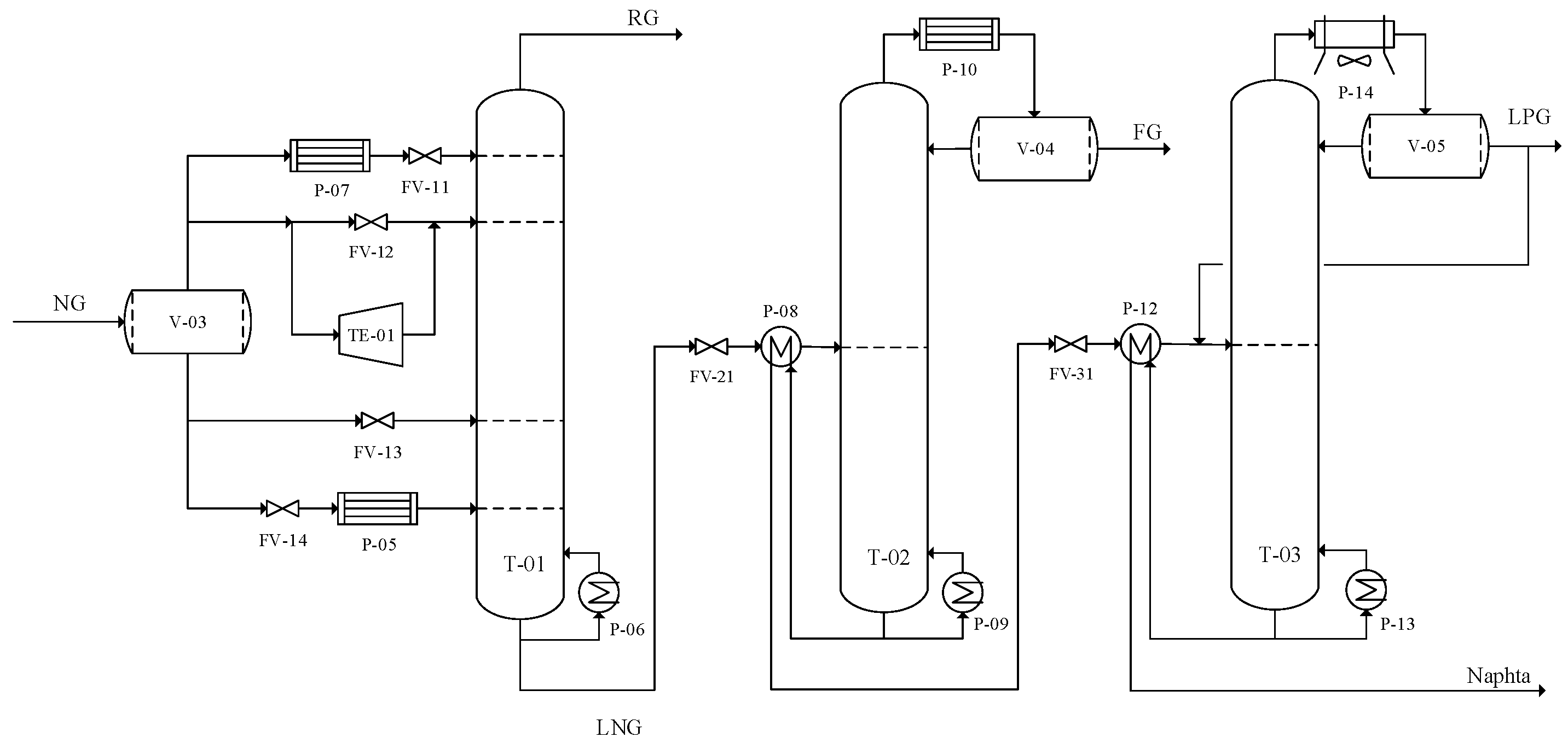
The RTO system developed in the present study was applied to an industrial Natural Gas Processing Unit (NGPU) owned by Petrobras in Brazil. In general terms, the unit is responsible for processing the NG from different sources to produce Residue Gas (RG), Fuel Gas (FG), Liquefied Petroleum Gas (LPG), and a stream containing components heavier than pentane, here denoted as Naphtha. Several unit operations are carried out in sequence—to name a few: NG dryier, Demethanizer, RG compressor, Deethanizer, and Debutanizer. These operations are supported by a Propane Refrigeration System and a Thermal Oil Heating System.

Initially, the collected NG with controlled admission pressure is cooled. Then, the gas follows to molecular sieves units where it is dried. The dry gas is then routed to the fractioning section, which corresponds to the feed of the simplified scheme illustrated in Figure 3.

This section is mainly composed by three separation units: T-01, in which RG is produced; T-02, which produces FG; and T-03, in which LPG and Naphtha are produced. In the first section, the dry gas is flashed into two vapor streams and two liquid streams. The first vapor stream is totally condensed and injected at the top of the Demethanizer column, acting as a reflux stream. The second vapor stream is divided into two streams, the main one is expanded in the turboexpander in order to reach even lower temperatures and the other goes to the Joule–Thomson valve, which is normally closed. These streams are then mixed and injected into the top section of the column. The fist liquid stream is injected directly as a feed-side stream at the bottom section of the column, while the other is first used in an energy integration scheme, being partially vaporized, and is then also injected into the bottom section of the column. It is noteworthy that all heat exchangers illustrated in Figure 3, upstream of T-01, are part of a single cold-box, heat integration scheme that is mischaracterized in the flowchart.

The top product of the T-01 is a methane-rich gas that is heated at the cold-box in the heat integration scheme and then sent to the compression stage associated with the turboexpander, while the bottom product, rich in components heavier than ethane, will then be fed to the Deethanizer tower—firstly passing though a flow control valve and a heat exchanger that energetically integrates the bottom product with the feed streams of the column. This unit is designed to operate in two modes depending on the current specification of the ethane in the LPG stream. With the low content of ethane in LPG, the condenser of T-02 works with the Propane Refrigeration System in order to produce the FG stream. On the contrary, the refrigeration is kept shut-down and the column loses its separation function, working only as an accumulation tank in the process. During the execution of the present RTO project and its implementation test period, the Propane Refrigeration System was off and the tower T-02 worked only as an accumulation tank.

The feed of the Debutanizer tower comes from the bottom product of tower T-02, again, after passing through a flow control valve and a heat exchanger that energetically integrates the bottom product with the feed streams of the column. The top product of the column is condensed in an air-cooler condenser and directed to the reflux drum, where, besides the split between the reflux and product streams, there is also a third stream that is mixed with the feed of the tower—the recirculation stream. This stream was added to the project of the unit due to the need to specify a large range of ethane content in the LPG stream. However, currently, the tower operates with a lower feed flow as that designed, so the recirculation also contributes to enhance the tower’s hydraulics. The system presents relatively slow dynamics and is subjected to frequent disturbances, mostly in feed composition and ambient temperature.

3.1.1. Economic Interests of the Operation

The Natural Gas Processing Unit of the present application receives gas from different sources, mainly including offshore oil production. The continuity of gas processing is vital for the offshore plant to continue operating with a proper destination of the produced gas. As previously mentioned, column T-02 was acting only as an accumulator tank during the design and tests of the present work; therefore, the NGPU produced only RG, LPG, and Naphtha. According to the most frequent economic configuration, the product with greater market value is LPG, followed by Naphta, and than RG, which is commonly used as fuel in the Thermal Oil Heating System.

Hence, the economic objective is to determine the optimal operating point that is able to produce LPG with maximum efficiency, acting as follows:

• Minimizing the loss of propane at the top of the Demethanizer column;
• Maximizing the content of ethane in LPG with respect to the established upper bound;
• Maximizing the content of pentanes in LPG with respect to the established upper bound;
• Minimizing the consumption of energy demanded by the process.

3.2. Process Model in PETROX

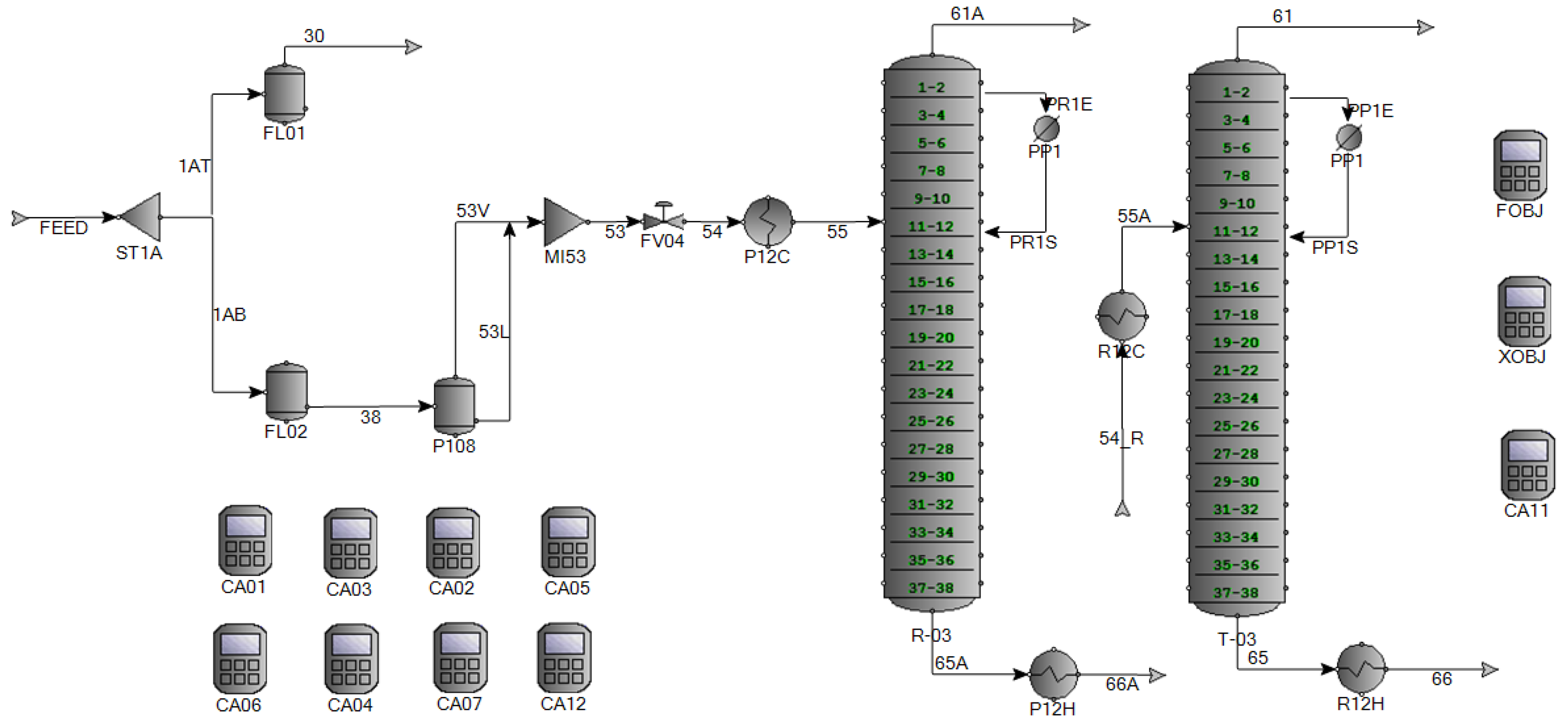
The scope of the present RTO application was defined to be the optimization of the Debutanizer column T-03; therefore, tower T-01 and tower T-02 were described in a simplified way. This choice was carried out following the philosophy of small-scale RTO in order to reduce computational cost and focus on optimizing the efficiency of the fractioning to produce LPG and Naphta. The model was developed in PETROX 3.8 following the “Modular Continuous with Successive Substitution” approach discussed in Section 2.1 and its flow sheet can be visualized in Figure 4.

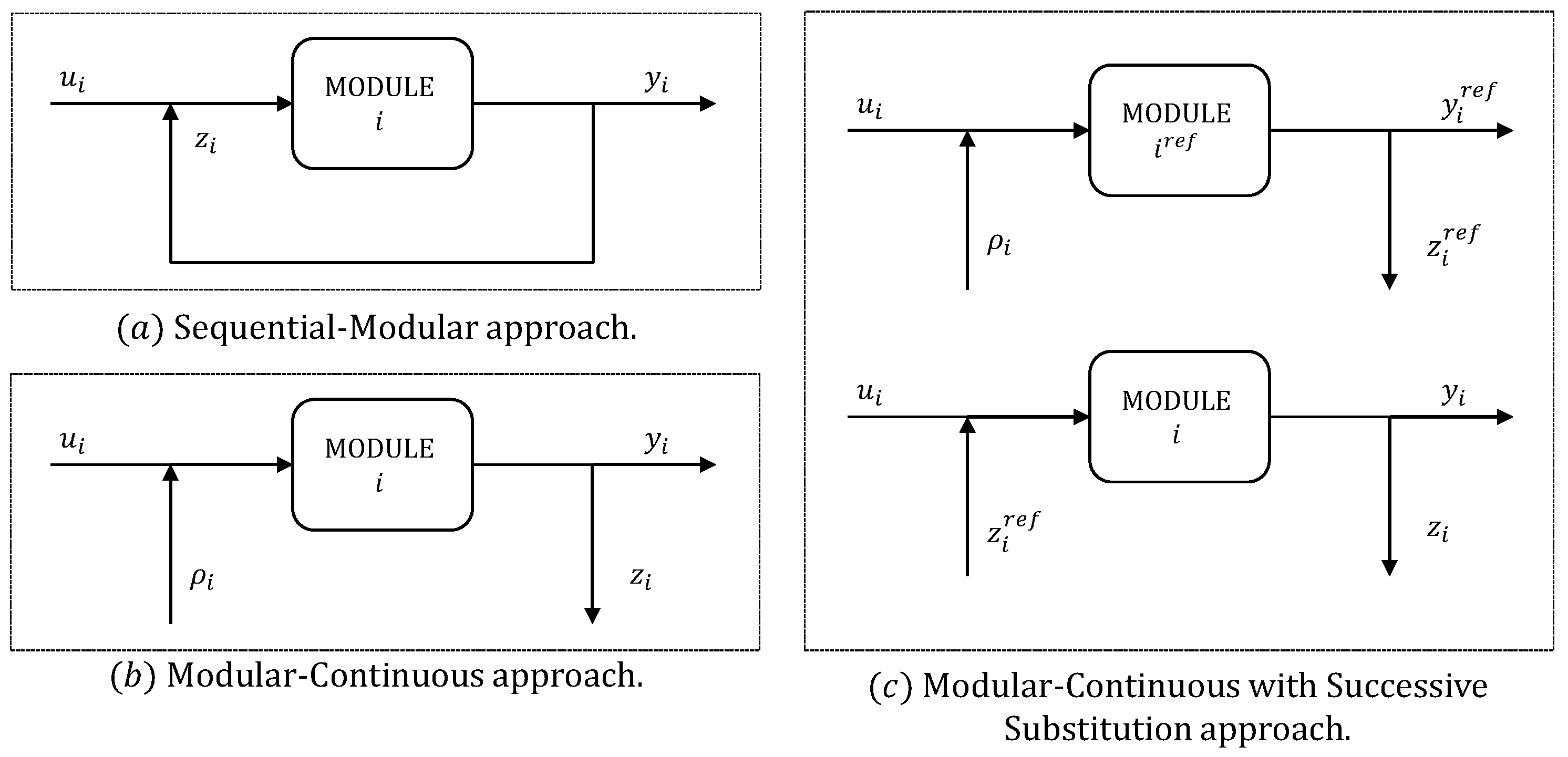
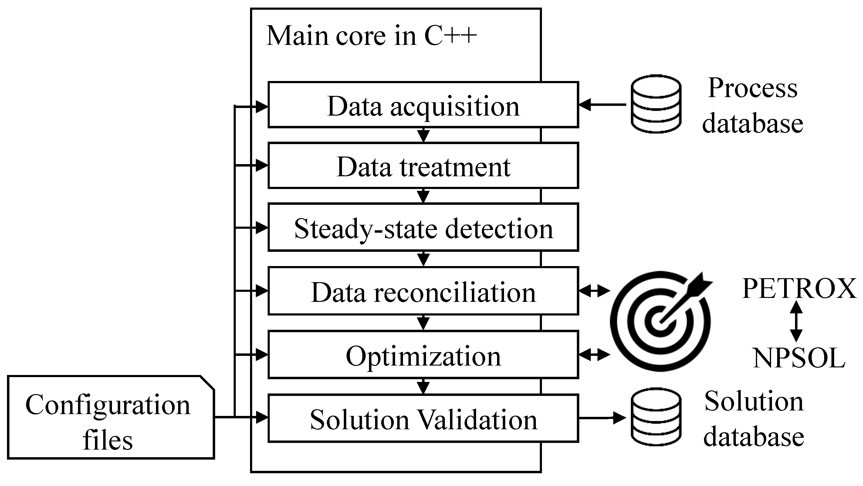
The input of data to the simulation is carried out by the several unconnected streams added to the simulation. The function of the calculators at the left-hand side of the flow sheet is to manage the information from the input streams to the main core of the simulation; they are also able to manage the information from a previous unit to a posterior unit. In addition, the function of the calculators at the right-hand side of the flow sheet is to manage the results of the simulation and to externalize results of interest, such as objective functions, nonlinear constraints, and output variables, for instance. Further description of the simulation calculators are provided in Appendix A.

The model has 13 components: nitrogen ($N_2$), carbon dioxide ($C{O}_2$), methane ($C1$), ethane($C2$), propane ($C3$), isobutane ($iC4$), n-butane ($nC4$), isopentane ($iC5$), n-pentane ($nC5$), n-hexane ($C6$), n-heptane ($C7$), n-octane ($C8$), n-nonane ($C9$). The simulation starts with the restoration of the feed stream; since the online chromatography is not complete, it does not discriminate compounds heavier than $C6$ and its measurements are not synchronized with the LPG analyzer, since there is an uncertain delay between these two analyzers. Therefore, the feed composition is parameterized to be estimated in the parameter estimation step. This is achieved by considering the components $C3$, $nC4$, and $iC4$ in such a way that the proportion between $C3$ and the sum of $nC4$ and $iC4$ can be controlled and the distribution between $nC4$ and $iC4$ would be the same as in the LPG composition:

$$\begin{array}{cc}\hfill & x_{C3}^{feed}=(x_{C3,m}^{feed}+x_{nC4,m}^{feed}+x_{iC4,m}^{feed}){\theta }_1\hfill \end{array}$$

(14a)

$$\begin{array}{cc}\hfill & x_{nC4}^{feed}=(x_{C3,m}^{feed}+x_{nC4,m}^{feed}+x_{iC4,m}^{feed})(1-{\theta }_1){\displaystyle \frac{x_{nC4,m}^{LPG}}{x_{nC4,m}^{LPG}+x_{iC4,m}^{LPG}}}\hfill \end{array}$$

(14b)

$$\begin{array}{cc}\hfill & x_{iC4}^{feed}=(x_{C3,m}^{feed}+x_{nC4,m}^{feed}+x_{iC4,m}^{feed})(1-{\theta }_1){\displaystyle \frac{x_{iC4,m}^{LPG}}{x_{nC4,m}^{LPG}+x_{iC4,m}^{LPG}}},\hfill \end{array}$$

(14c)

where $x_i^j$ and $x_{i,m}^j$ represent the molar composition of component i in the stream j in the simulation and measured, respectively; ${\theta }_1\in \{0,1\}$ is the estimated parameter to control the proportion between propane and butanes.

A similar strategy is applied to the heavier components of the feed stream that are not directly measured but lumped in the $x_{C6+,m}^{feed}$:

$$\begin{array}{cc}\hfill & x_{C6}^{feed}=x_{C6+,m}^{feed}(1-{\theta }_2)\hfill \end{array}$$

(15a)

$$\begin{array}{cc}\hfill & x_{C7}^{feed}=x_{C6+,m}^{feed}{\theta }_2{p}_{C7}\hfill \end{array}$$

(15b)

$$\begin{array}{cc}\hfill & x_{C8}^{feed}=x_{C6+,m}^{feed}{\theta }_2{p}_{C8}\hfill \end{array}$$

(15c)

$$\begin{array}{cc}\hfill & x_{C9}^{feed}=x_{C6+,m}^{feed}{\theta }_2{p}_{C9},\hfill \end{array}$$

(15d)

where ${\theta }_2\in \{0,1\}$ is the estimated parameter to control the proportion between $C6$ and the heaviest components, and $p_i$ is a typical proportion between component i and the heaviest components obtained from lab reports. The feed measurements are directly used for the other components.

The description of the Demethanizer model was carried out by a simplified approach similar to the proposition of Ito et al. [50]. In order to reduce complexity and computational cost, the tower is represented by a splitter and two flash drums to produce the two top and bottom product streams using, respectively, a dew point and boiling point flash units. A parameter is added to control the fractioning of T-01 considering the cut between ethane and propane. However, since the reflux of the column is injected directly at the top tray, part of the reflux stream is vaporized in the moment that it enters the tower, so the top product is not in fact in the dew point due to the mixture between the saturated vapor that comes from the first tray and the vaporized portion of the reflux stream. Therefore, to account for this modeling characteristic, the top temperature cannot be used as a reconciliation variable and more importance is given to the measurement of the $C3$ content in the RG stream and the content of $C2$ and $C3$ in the LPG stream. With a simple mass balance, it is possible to fully specify the split flow rates considering the loss of $C3$ in the RG stream and the flow rates of $C2$ and $C3$ in the LPG stream:

$$\begin{array}{cc}\hfill & r_{C2/3}={\theta }_3{\displaystyle \frac{x_{C3,m}^{LPG}}{x_{C2,m}^{LPG}+x_{C3,m}^{LPG}}}\hfill \end{array}$$

(16a)

$$\begin{array}{cc}\hfill & F_{C3}^{RG}=x_{C3,m}^{RG}(F_{N_2}^{feed}+F_{C{O}_2}^{feed}+F_{C1}^{feed}+F_{C2}^{feed}-r_{C2/3}{F}_{C3}^{feed})\hfill \end{array}$$

(16b)

$$\begin{array}{cc}\hfill & F_{C2}^{LNG}=r_{C2/3}(F_{C3}^{feed}-F_{C3}^{RG}),\hfill \end{array}$$

(16c)

where $F_i^j$ corresponds to the molar flow rate of component i in stream j, $r_{C2/3}$ is the ratio of the fraction of $C3$ in the LPG stream over the sum of the fractions of $C2$ and $C3$ in the LPG stream and ${\theta }_3\in \{0,1\}$ is the parameter responsible for adjusting the fraction of $C3$ in RG and $C2$ in LPG. The superscript LGN refers to the bottom product of tower T-01 that feeds tower T-03. This strategy is able to match the loss of $C3$ in the RG with the plant measurements. Additionally, as during the estimation of ${\theta }_3$, the value of Equation (16c) might be negative, a constraint is added to prevent this value from being negative.

The LNG stream passes through an expansion valve upstream of the feed preheat exchanger (P-12) of the T-03. This heat exchanger is simulated in three steps in order to avoid any loop that would include excessive iterations in the simulation. In the first step, the simulation receives the input of the heat duty of the cold side (${\rho }_1$), which is a decision variable added by the MCSS approach, and then goes to a reference tower to simulate an approximation of the T-03 because the energy balance in the feed heat exchanger is not satisfied. Then, the hot side of the feed heat exchanger is simulated by an HOCI (hot-out cold-in) temperature difference approach based on the bottom product of the reference tower. This HOCI approach is added in order to enhance the robustness of the simulation, avoiding physical inconsistencies in the temperature differences. The difference between the outlet and the inlet temperatures are calculated from measurement, and this difference is summed to the inlet temperature calculated by the simulation to produce the outlet specification of the hot side of the heat exchanger. After the heat duty calculation, the cold side is simulated again specifying the heat duty of the hot side and then the T-03 tower is properly simulated. It is important to highlight that each heat exchanger must be analyzed individually and, here, the HOCI approach is appropriate because the flow rate of the hot fluid will always be inferior to the flow rate of the cold fluid.

The recirculation stream is also simulated by a pump-around in order to avoid unwanted loops. A parameter is added to vary the Murphree efficiency of the inner trays of the tower, so that the internal profile of the tower may approximate the measured internal profile. The reboiler and condenser efficiencies are kept fixed and equal to 1. The flow rates of the reflux, recirculation, and bottom product were chosen as specifications of the tower to improve robustness, since choosing temperatures might reduce the chances of converging the simulation considering the whole operational range.

Finally, the pressures were defined following a backpressure propagation strategy. The final pressure points were specified accordingly to the measurements for the top pressure of T-01 and the condenser pressure of T-03 and these pressures were back-propagated by typical pressure drops of the system. This approach showed to be very efficient for this case study due to the larger values of pressures compared with the values of pressure drops.

It is important to highlight that all modeling choices were considered in order to provide a suitable model developed in a sequential-modular simulator for optimization purposes. Therefore, all excessive iterations of numerical methods are avoided and the main responsibility of converging the model is given to the optimization layer, or through the addition of constraints, either through a successive substitution generated naturally by the several calls of the model function by the optimization algorithm.

3.3. Formulation of the Data Reconciliation Problem

The formulation of the objective function for the data reconciliation simultaneously with parameter estimation was carried out in a weighted least squares estimator with normalized variables:

$${\mathcal{J}}_{rec}=\sum _{i=1}^{n_{y_r}}{w}_i^y{\left({\displaystyle \frac{y_{k,i}^m-y_i^{rec}}{y_{k,i}^m}}\right)}^2+\sum _{i=1}^{n_{u_r}}{w}_i^u{\left({\displaystyle \frac{u_{k,i}^m-u_i^{rec}}{u_{k,i}^m}}\right)}^2,$$

(17)

where ${\mathit{w}}^y\in {\mathbb{R}}^{n_{y_r}}$ and ${\mathit{w}}^u\in {\mathbb{R}}^{n_{u_r}}$ are weight vectors of the output and input variables, respectively.

Table 1. Measured output variables.

Variable Description	Weight (${\mathit{w}}^{\mathit{y}}$)
Volumetric fraction of $nC5$ and $iC5$ in LPG	${10}^3$
Top temperature of tower T-03	${10}^4$
Bottom temperature of tower T-03	${10}^5$
Condenser temperature of tower T-03	${10}^5$
Fraction $C3/(nC4+iC4)$ in LPG	${10}^4$
Temperature of the control tray of tower T-03	${10}^4$

presents the measured output variables and their respective weights considered in the objective function.

As previously commented, the developed model specifies the $C3$ loss in the RG stream given the chromatographic measurement, so this value cannot be reconciled. The top temperature and the volumetric fractions of $nC5$ and $iC5$ are considered reconciled variables. Both of these measurements compete to specify the top of tower T-03, since they represent the same information in essence. In Table 1, more importance is given to the top temperature rather than the analyzer, because the analyzer has lower measurement frequency and is potentially more noisy. The bottom temperature of tower T-03 is an estimated output that is influenced by the content of heavier components of the feed stream, which is controlled by adjusting parameter ${\theta }_2$. Similarly, the condenser temperature is an estimated output that is influenced by the content of $C2$ in the LPG stream; this composition is controlled by adjusting parameter ${\theta }_3$, which represents the cut between $C2$ and $C3$ in tower T-01. The fraction $C3/(nC4+iC4)$ in LPG is also an estimated output; this variable is influenced by the ratio between propane and butanes in the feed stream, which is controlled by the parameter ${\theta }_1$. Finally, the temperature of the control tray is an estimated output controlled by the Murphree efficiency of the column.

Table 2. Input variables and parameters for the data reconciliation simultaneous with the parameter estimation problem.

Degree of Freedom	Weight (${\mathit{w}}^{\mathit{u}}$)	Lower Bound	Upper Bound
Bottom flow rate of tower T-03 (kmol/h)	−	0	100
Reflux flow rate of tower T-03	${10}^2$	DCS	DCS
Recirculation flow rate of tower T-03	${10}^2$	DCS	DCS
Murphree Efficiency of tower T-03	−	0.8	1
Heat duty of P-12 ${\rho }_1$ (Mcal/h)	−	10	500
Parameter ${\theta }_1$	−	0	1
Parameter ${\theta }_2$	−	0	1
Parameter ${\theta }_3$	−	0	1

presents the input variables and parameters considering degrees of freedom in the reconciliation simultaneously with the parameter estimation problem, their bounds, and their weights in the objective function, in the case where measurements are available. It is important to highlight that when the abbreviation DCS is assigned for a bound value, this value is defined by the operator in the Digital Control System (DCS) of the plant. The specific values of the limits defined in the DCS are not disclosed because these limits varied considerably during the analyzed time period. The flow rates of the column (bottom, reflux, and recirculation) are considered degrees of freedom to specify the column variables. For the reflux and recirculation streams, the available volumetric measurements are uncertain, so these variables are also reconciled but with smaller weights than the reconciled outputs, so the optimization may have more flexibility to deviate from the measurements.

Table 3. Constraints of the Data Reconciliation Problem.

Constraint Description	Lower Bound	Upper Bound
Molar fraction of $C4-$ in Naphta	0	0.015
Pressure loss on the feed valve of T-03 (kgf/cm2)	1	∞
Ratio of $C2/C5+$ in LPG	0	16
Vapor flow rate after flash P108	0	0
Molar flow rate of $C2$ in LNG	0	∞
Heat duty difference of cold and hot side of P-12	0	0

presents the constraints of the data reconciliation problem and their bounds.

The added constraints are the minimum requirements to guarantee that the simulation converges in an expected way. This is achieved by forcing the pressure loss on the valve upstream from the T-03 to be greater than 1 kgf/cm², guaranteeing that the molar flow of $C2$ in the LNG stream is greater than 0, as already discussed in Section 3.2, and making sure that the liquid product stream of the flash P-08 is saturated; this flash unit is downstream of tower T-01. In addition, the constraints in the maximum molar content of components lighter than $C4$ ($C4-$) to be $0.015$ and in the ratio of the composition of ethane and components heavier than pentanes ($C2/C5+$) to be less then 16 are redundancies to guarantee product quality requirements. Finally, the last constraint is added due to the MCSS approach in order to guarantee the energy balance upon convergence of the optimization.

3.4. Formulation of the Optimization Problem

In order to meet the economic interests of the operations described in Section 3.1.1—except for objective 1, which would require a more detailed model for the system of column T-01—the following objective function was designed:

$${\mathcal{J}}_{opt}={\displaystyle \frac{1}{W_{-C2}^{LNG}}}\left(p^{LPG}{W}^{LPG}+p^N{W}^N-p^{RG}{\displaystyle \frac{Q_r}{\eta {\mathrm{LHV}}^{RG}}}-p^E{Q}_c\right),$$

(18)

where $p^{LPG}$, $p^N$, $p^{RG}$, and $p^E$ represent the price per unit of mass of LPG, Naphta, RG, and electric energy, respectively; $W_{-C2}^{LNG}$ is the mass flow rate of LNG free of ethane that feeds tower T-03; $W^{LPG}$ and $W^N$ are, respectively, the mass flow rates of LPG and Naphta streams; $Q_r$ and $Q_c$ are the heat flow rates of the reboiler and condenser of the tower T-03, respectively; $\eta$ is the efficiency of the thermal oil furnace; and ${\mathrm{LHV}}^{RG}$ is the lower heat value of the residue gas used as fuel.

The idea of the developed objective function is that the optimization may be able to maximize the efficiency of the fractioning process of the column for a given feed flow rate. That is the reason for dividing the expression by the mass flow rate of the LNG stream free of ethane. This value should be free from C2 because the content of ethane in the LNG stream is a decision variable of the problem, so it could take the wrong path minimizing this variable.

The decision variables, or degrees of freedom, of the optimization problem are presented in

Table 4. Decision variables of the Optimization Problem.

Decision Variables	Lower Bound	Upper Bound
Bottom flow rate of tower T-03 (kmol/h)	0	100
Reflux flow rate of tower T-03	DCS	DCS
Recirculation flow rate of tower T-03	DCS	DCS
Condenser Pressure	DCS	DCS
Heat duty of P-12 ${\rho }_1$ (Mcal/h)	10	500
Parameter ${\theta }_3$	0	1

, as well as the respective bounds.

Besides the constraints used in the data reconciliation problem, which are presented in Table 3, the optimization problem has additional constraints, as presented in

Table 5. Additional constraints of the Optimization Problem.

Constraint Description	Lower Bound	Upper Bound
Volumetric composition of $C2$ in LPG	DCS	DCS
Volumetric composition of $nC5$ and $iC5$ in LPG	DCS	DCS
Condenser Temperature (${}^{°}$C)	30	∞
Temperature of the control tray of tower T-03	DCS	DCS
Bottom temperature of tower T-01	DCS	DCS

.

The volumetric composition of ethane and pentanes have different specification values defined by the operation. These specifications are provided by the technical team of the operation in the DCS and the optimization must respect them. A constraint is added to the value of the condenser temperature; as it is an air-cooler, in which the cold fluid is air at ambient temperature, it would not be reasonable to allow the temperature of the hot fluid at the outlet to be inferior to 30 ${}^{°}$C. Even though this temperature is also constrained by the composition of C2 in the LPG stream, this redundancy is added in order to prevent the solution from finding an unreachable temperature.

In addition to those constraints, two more are added with respect to safety operational limits defined by the operator in the DCS—one for the temperature of the control tray of T-03 and another at the bottom temperature of T-01. It is worth mentioning that this last constraint is another redundancy with the content of C2 in the LPG stream, as the bottom stream of T-01 is saturated and its temperature depends mostly on the content of the lighter component—C2 in this case.

3.5. Integration between RTO and the DCS

The purpose of this paper is not to deeply describe the control system of the unit. However, some points are interesting to be noted in order to clarify how the integration between the RTO and the DCS is carried out.

The regulatory control system is composed by a multiloop single-input single-output PID controller mainly designed with cascades feedback loops. The operation team of the plant can decide whether to manually define the setpoints of these controllers or to turn on the supervisory control layer. This supervisory control layer is a model predictive controller that solves an optimization problem aiming to minimize the quadratic deviation between the measured outputs and inputs from reference trajectories and target trajectories, respectively, subjected to input–output models and constraints. The algorithm uses the step response model and is based on the DMC algorithm proposed by Cutler and Ramaker [51]. However, the algorithm was modified to account for an adaptive strategy that is able to adjust the internal model of the MPC based on the current operational condition of the plant.

Above the MPC layer, there is a simple optimization layer that aims to maximize an economic objective function subjected to the same adaptive input–output model of the MPC layer, resulting in quadratic programming (QP). When the loop of the RTO is closed to the supervisory control layer, which is also a decision of the plant operator, that simple optimization layer becomes an intermediate QP problem between MPC and RTO, as proposed by Rotava and Zanin [52]. Therefore, when the RTO is in closed loop, the intermediate optimization problem aims to minimize the distance between the solution of the RTO and the achievable values based on the input–output model of the MPC. This is a way to translate the solution of the economic optimization subjected to a detailed nonlinear model to the space of linear models, preventing infeasible targets to be sent to the control layer.

The chosen variables to perform the integration were the content of ethane and pentanes in LPG, the reflux and recirculation of T-03, and the bottom temperature of T-01.

3.6. Estimation of the Economic Return

The economic return was evaluated following the novel methodology proposed in Section 2.3. The profit function was defined as the sum of the incomes with products minus the costs with Natural Gas:

$${\mathcal{J}}_{profit}=p^{LPG}{W}^{LPG}+p^N{W}^N+p^{RG}{W}^{RG}-p^{NG}{W}^{NG},$$

(19)

where $p^{NG}$ and $W^{NG}$ are the price per mass unit and mass flow rate of the Natural Gas stream, respectively.

Three data windows were collected for the analysis of each operation mode, as defined in Section 2.3, and a data treatment was performed to remove any gross errors, outliers, and regions where the unit was not operating, resulting in the following:

• Regulatory control—an interval of 97 days of operation resulting in 60,350 points with a sampling time of 2 min;
• Supervisory control—an interval of 138 days of operation resulting in 20,583 points with a sampling time of 2 min;
• Optimization—an interval of 96 days of operation resulting in 49,043 points with a sampling time of 2 min.

In the three data windows, the variables frequently violate the allowable bounds due to measurement noise. Although this violation was expected, it is alarming, especially for the upper bounds of the content of ethane and pentanes in the LPG stream, since values above these upper bounds would result in values of the profit function greater than the optimum solution. This effect would enable the performance index to be greater than 1, which is unacceptable. Hence, all points above these upper bounds were excluded from the analysis for the supervisory and optimization operating modes, resulting in the removal of 28.5% of the points in the supervisory data window and 24.8% of points in the optimization data window. However, in the regulatory mode, the bounds of the manipulated and output variables were not well specified in the system, since in this mode, the operation team is mainly focused in the PID’s setpoints. So, these bounds were arbitrarily chosen in order to remove some percentage of points from the analysis. As it is expected that the variability of data would be higher in the Regulatory control, this percentage was conservatively chosen as equal to the RTO data window.

Another issue that hinders the effort to calculate the performance index is that in the regulatory and supervisory control modes, the RTO was not operating in open loop. Therefore, no results of the data reconciliation and the optimization problem were available. Therefore, in order to enable the analysis, a mass balance spreadsheet was developed in order to calculate the profit function for all points in each operation mode, in which the reconciled solutions were obtained by the use of the available chromatography measurements and the optimal solutions were approximated using the upper bounds as desirable specifications. This way, the computation of the performance index was made possible regarding the specificity of each operating condition.

4. Results and Discussion

In the following, the results presented in Section 4.1 and Section 4.2 are related to the first month of the RTO’s operation. It is noteworthy that no fixed time frequency was set for the RTO run time. Instead, RTO runs in its own variable frequency, depending on the computational cost to run each iteration. This practice is usually avoided by commercial applications aiming not to excessively disturb the supervisory controller with frequent changes of reference values and targets. In the present study, this fact is not an issue due to the fact that the MPC controller is imbued with constraints of minimal movement, which prevents sudden transients. Additionally, due to the nondisclosure agreement with the industrial partner, the results are presented in a normalized form.

4.1. Data Reconciliation

This section presents the results related to the simultaneous data reconciliation and parameter estimation problem. As the RTO ran $N=920$ times within the 30-day window herein analyzed, only a fragment of the data window is provided to compare the plant data with the reconciled value in the figures of this section. Therefore, in order to have a sensibility of the whole picture, a relative average error in percentage was calculated for each variable of interest as follows:

$${ϵ}_i^y(\%)={\displaystyle \frac{100}{N}}\sum _{k=1}^N{\displaystyle \frac{|y_{k,i}^m-y_i({\overline{\mathbf{\theta }}}_k,\mathit{u}({\overline{\mathit{u}}}_k^{rdf}))|}{|y_{k,i}^m|}},$$

(20)

where ${ϵ}_i^y$ is the relative average error of output i. The error of the reconciled inputs is calculated analogously.

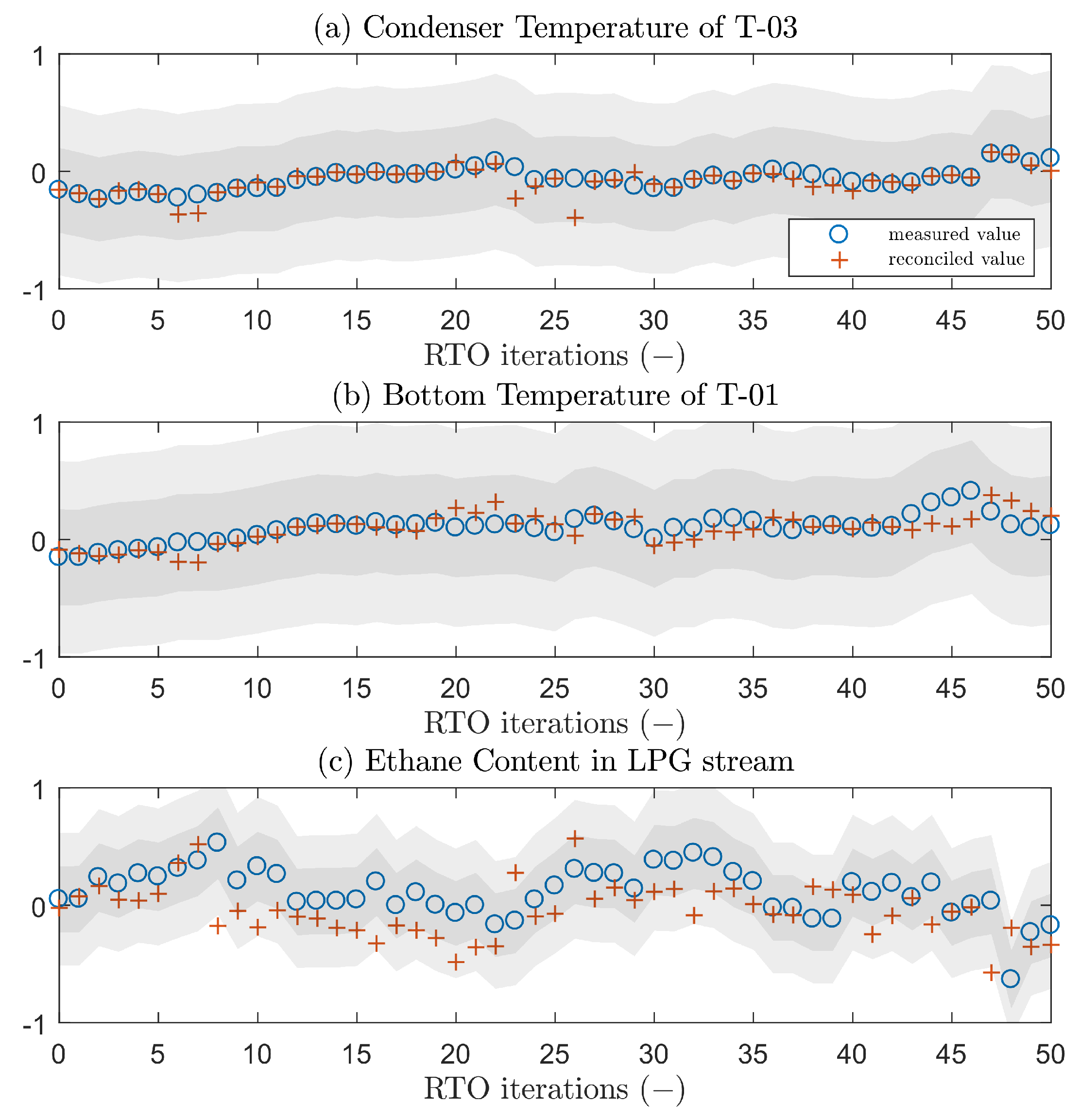
Figure 5 illustrates the results related to the content of ethane in the LPG stream—that is, the condenser temperature of T-03, the bottom temperature of T-01, and the volumetric fraction of ethane in LPG itself. The dark-gray regions around the plant data points represent a deviation of $\pm 5\%$ of the plant data at instant k, while the light-gray represents a deviation of $\pm 10\%$. For this set of variables, it is interesting to note that only the temperature of the condenser of tower T-03 is considered in the objective function of the problem and the other two are adjusted as a consequence of it. The relative error of these variables are $0.63\%$, $1.34\%$, and $3.81\%$, respectively. The higher error on the volumetric fraction was expected since this measurement has a low sampling frequency and considerably high noise.

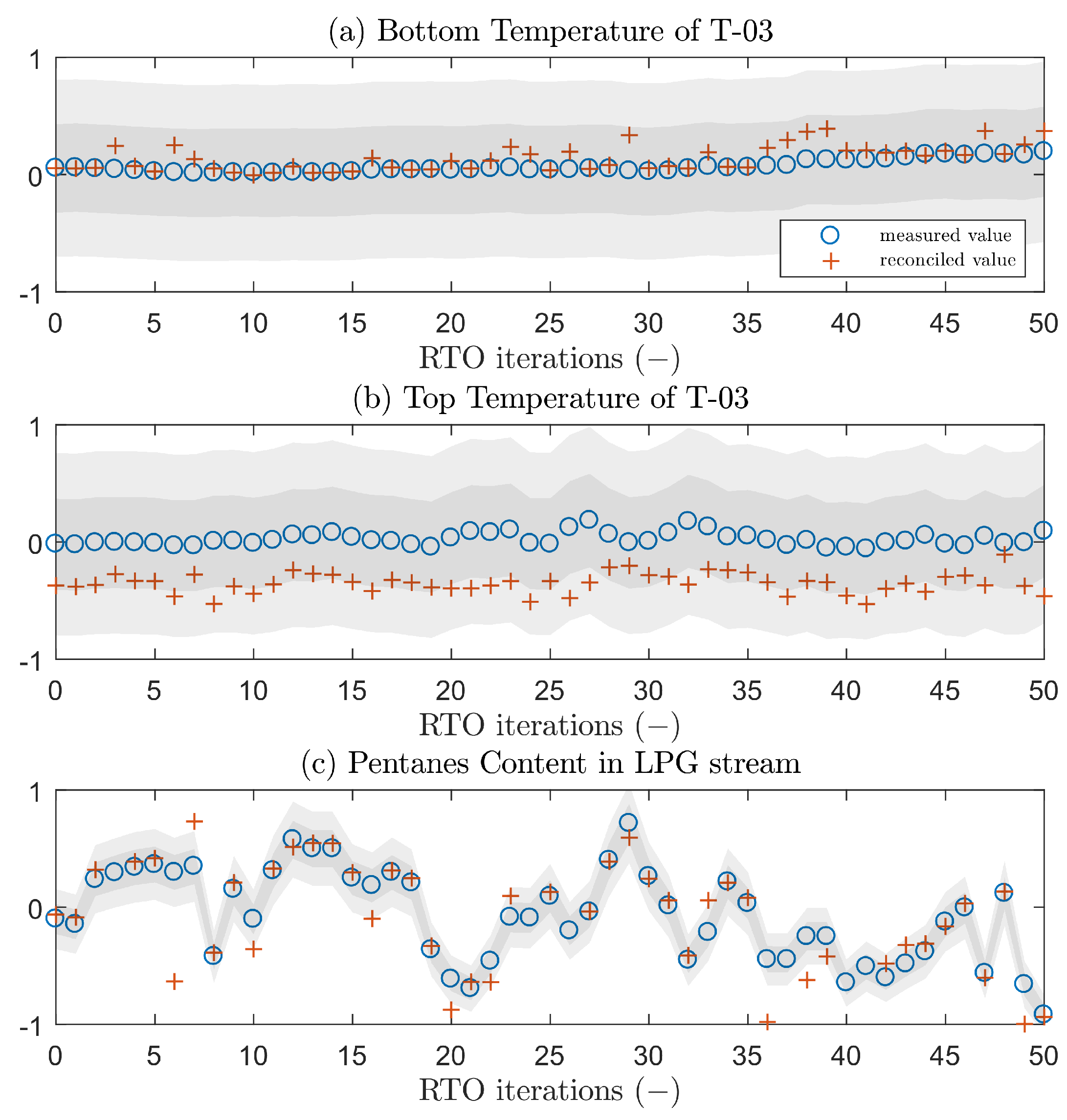
Figure 6 shows the result of the bottom temperature of T-03, which presented a low relative error of $0.60\%$. This result is a consequence of the estimation of the content of the heavier components, which are not measured. Figure 6 also illustrates the variables that are related to the content of pentanes in LPG, which are the top temperature of column T-03 and the volumetric fraction of pentanes in LPG; both variables were reconciled.

The relative error of the top temperature was $4.01\%$, while the error of the volumetric fraction of pentanes was $7.84\%$. Moreover, a bias is observed in the reconciled top temperature value, consistently remaining below the plant data, which can be explained by the position of the sensor near the second tray. The sensor may be presenting interference due to the higher temperature of the tray below; therefore, the use of another temperature sensor will be considered in the future.

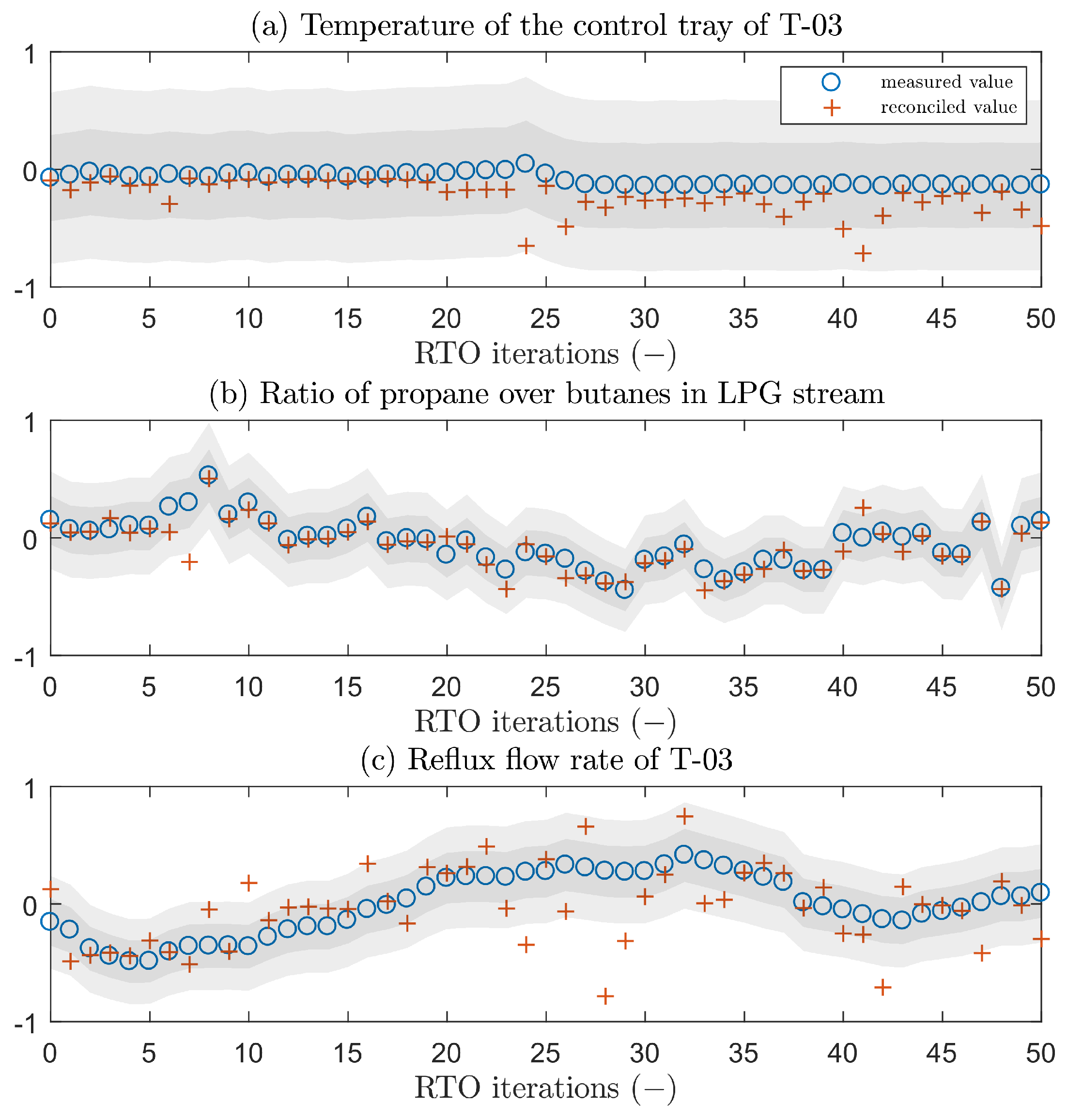
Figure 7 shows the results of the temperature of the control tray of tower T-03, the ratio of propane over butanes in LPG, and the reflux flow rate.

The temperature of the control tray of T-03 is an estimated output variable that is adjustable by the estimation of the Murphree efficiency of the column, which explains the low relative error of $1.97\%$ of this variable. In addition, the ratio of propane over butanes in the LPG is also an estimated output, which is adjusted by the manipulation of the ratio of propane over butanes in the feed stream of the process; this variable presented a relative error of $2.12\%$. Lastly, the reflux flow rate of tower T-03 is an estimated input, but a relatively low weight is assigned to this variable due to a high uncertainty in the measurement of the liquid streams. However, even with this uncertainty, an error of $5.02\%$ is considered low.

The results herein presented attest to the quality of the developed model and its ability to represent the variables of the system. Therefore, the model is adherent to plant in study.

4.2. Optimization

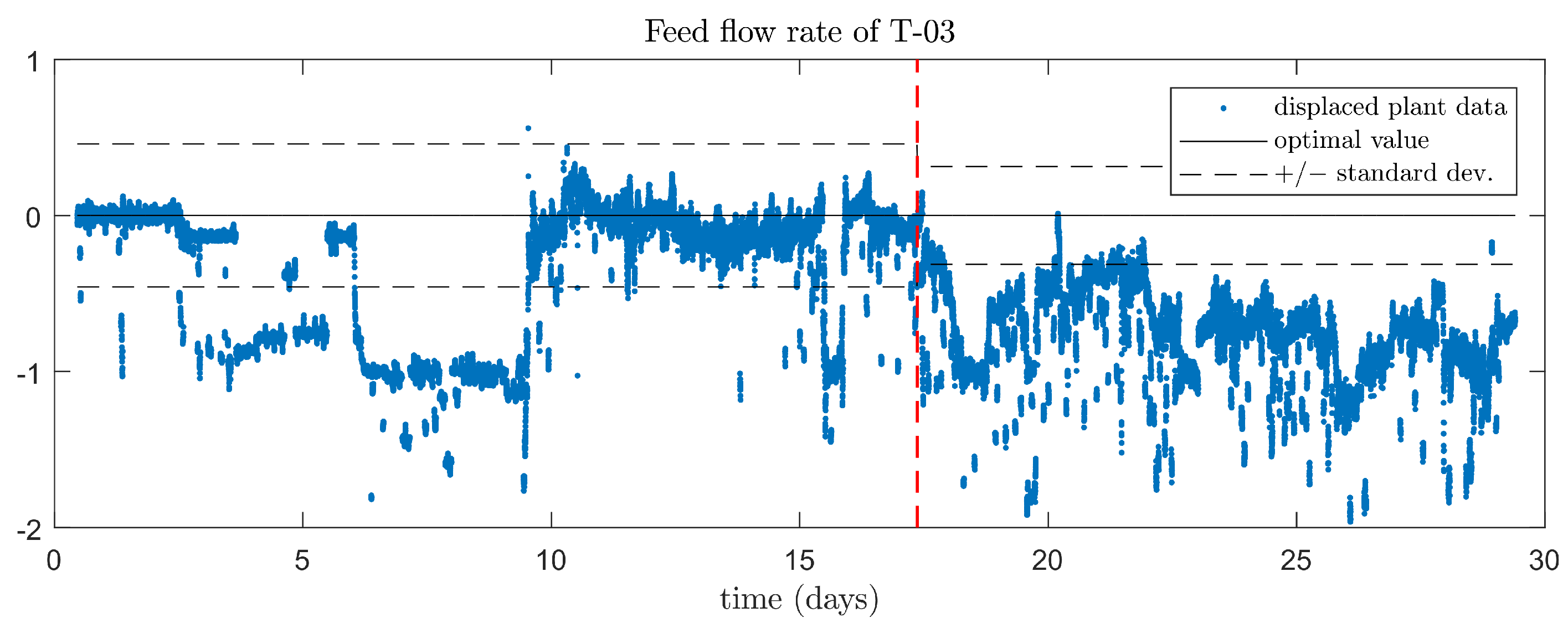
During the first month of RTO operation, there were two moments that are delimited in the results of this section. First, the RTO was set to run in open loop with the DCS, so its behavior could be observed and any required adjustment could be made. Then, after approximately 17 days of operation, the RTO loop was closed with the DCS—that is, the control system started reading the solution of the RTO and tracking the optimal operation.

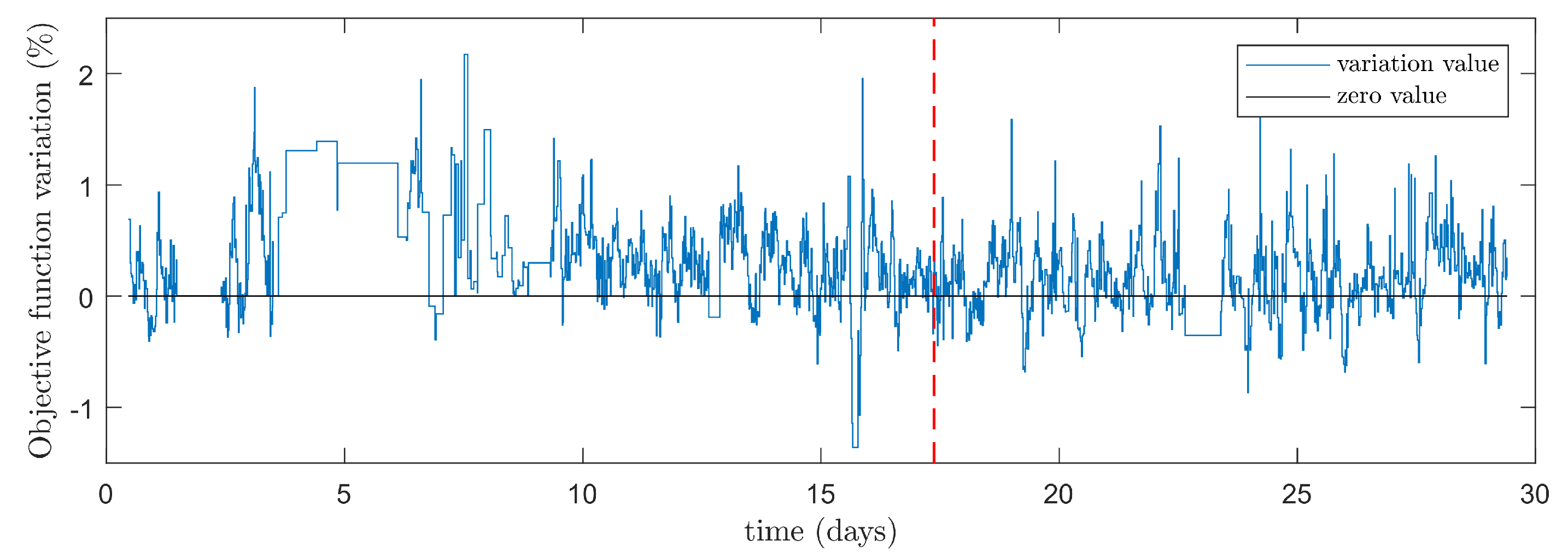
Figure 8 shows the result of the objective function variation in percentage, that is, the optimal value of the objective function minus the value calculated in the reconciliation problem over this last value. The vertical dashed line indicates the moment when the RTO loop was closed.

The zero line is marked to denote the boundary between actual economic gain or loss provided by the optimal solution. When the value is positive, there are economic gains, otherwise there are economic losses. It is possible to see that there is a considerable number of times that the optimization crossed the zero line to the economic loss region. However, this can be explained by the violation of the constraints where the plant may operate, so the optimization may decide to reduce the economic gain in order to bring the plant back to a feasible region. Despite this fact, the overall economic gain is achieved and is verified by a positive value on the numerical integration of the curve.

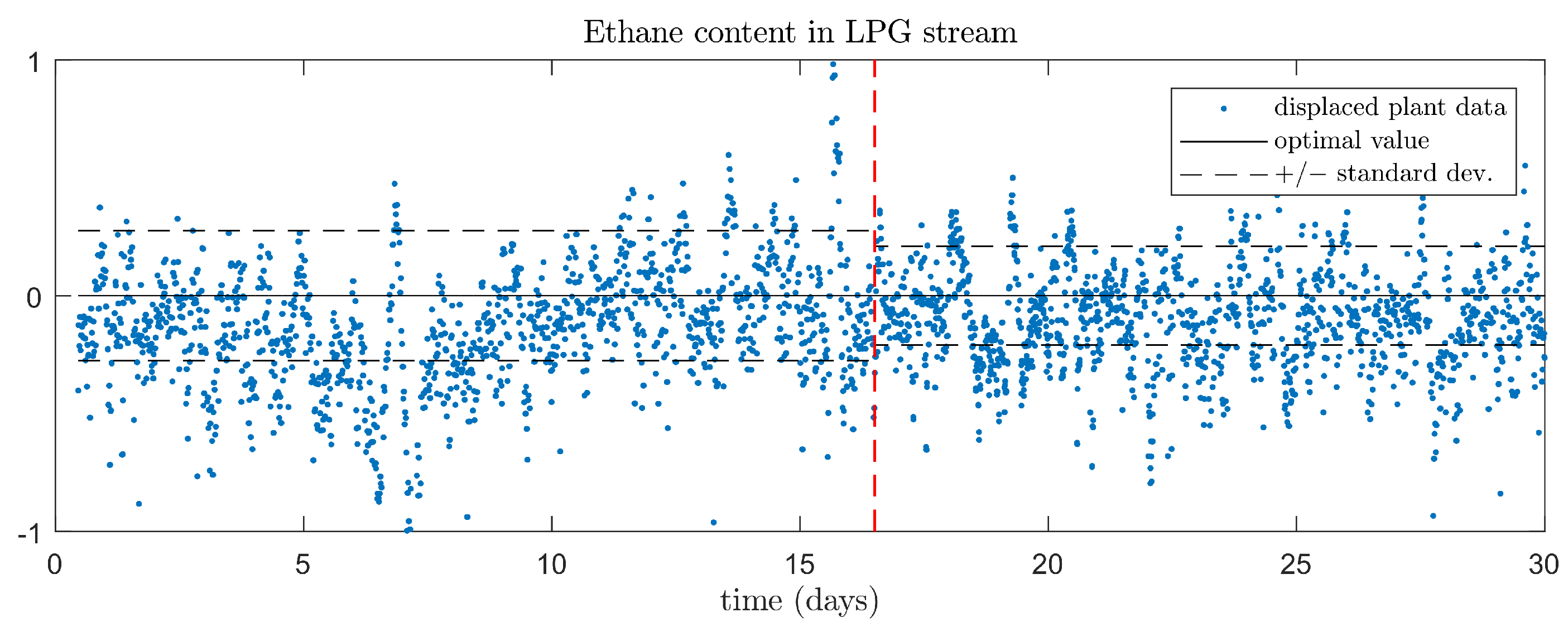
Figure 9 shows the trend of the volumetric fraction of ethane in LPG displaced by the optimal value, which is the most sensitive variable in the economic function. The horizontal dashed lines illustrate the resultant standard deviation upward and downward in both time windows. The results show that the content of ethane, which is sent to the DCS as a reference value, was more concentrated around the optimal value after closing the loop of the RTO, with a reduction of $31.9\%$ on the standard deviation value.

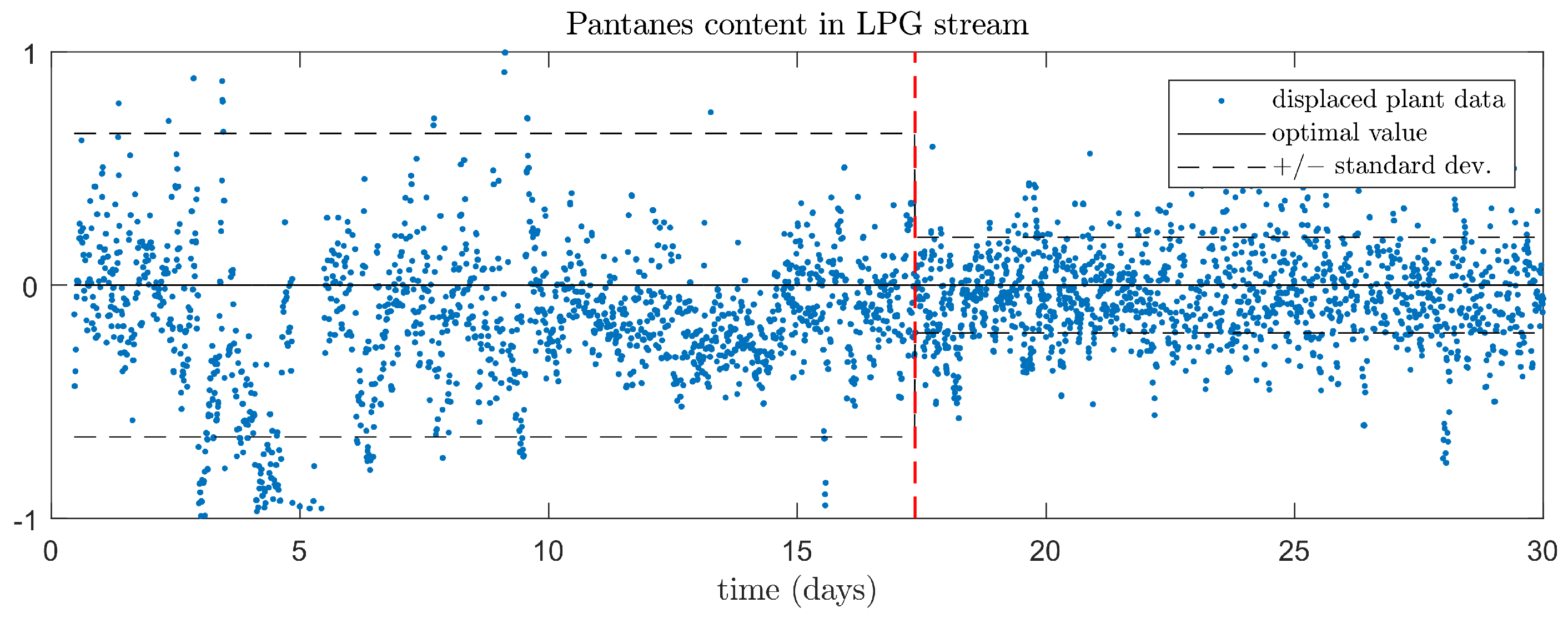
Figure 10 illustrates the result related to the content of pentanes in the LPG stream, which is sent to the DCS as a reference value. This result shows a high concentration of the data points around the optimal value, with a reduction of $217\%$ in the standard deviation value after closing the loop—the right-hand section after the vertical dashed line. This result reinforces the operational benefits resulted from the implementation of the RTO.

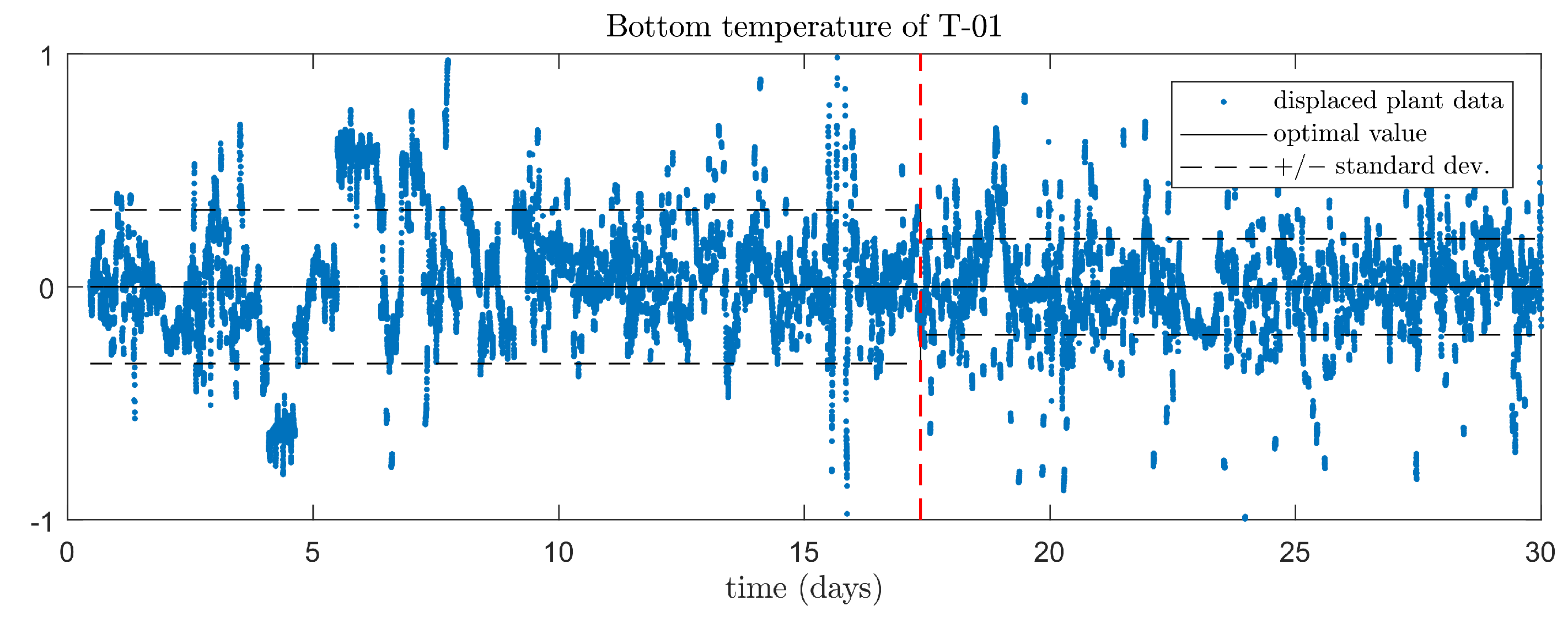
A similar result is also observed in the bottom temperature of tower T-01, as showed in Figure 11, and in the reflux flow rate, in Figure 12, with decreases in the standard deviation around the optimal values of $59.9\%$ and $19.7\%$, respectively. The bottom temperature of tower T-01 and the reflux flow rate are sent to the DCS as a reference value and a target, respectively.

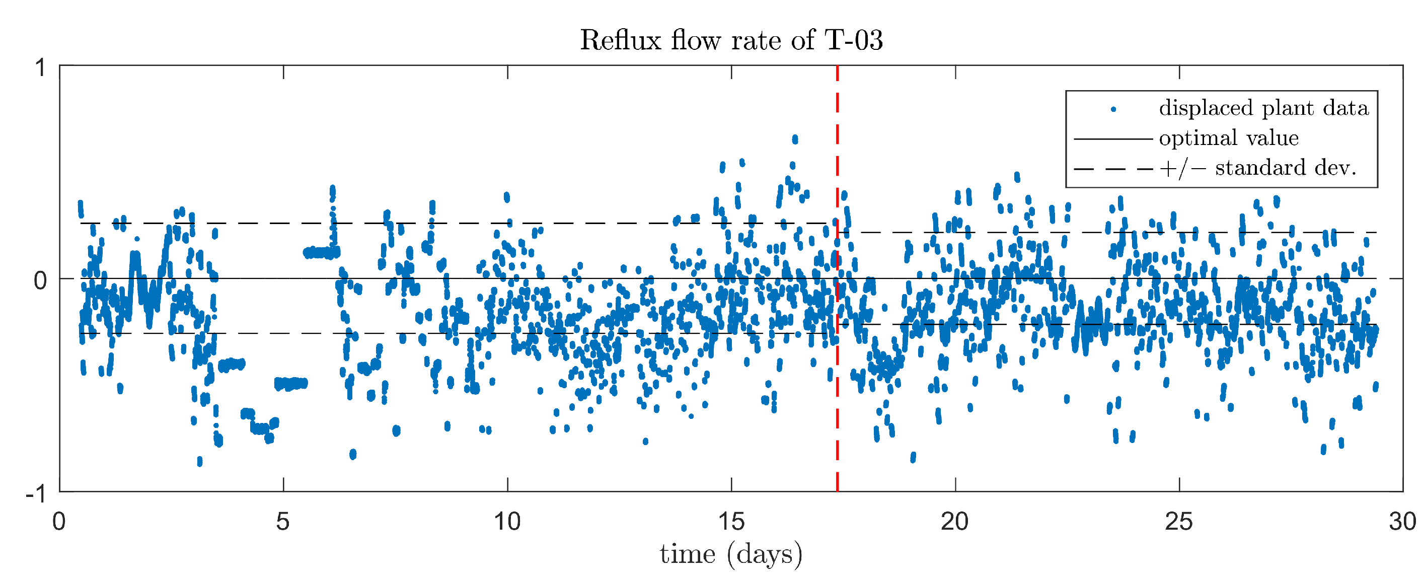
Regarding the recirculation flow rate, which is sent as a target to the DCS, it possible to see in Figure 13 that, even though there is a decrease in the standard deviation around the optimal value of $19.7\%$, the data points kept consistently below the optimal value. This suggests that the control layer may be neglecting the optimal target of this variable and adjustments must be carried out in the future.

The results shown support the fact that the RTO provides an economic benefit by the positive variation of the objective function and also provides an operational benefit by the reduction of the variability of the data points. In general, the communication between RTO and the control layer was successfully achieved.

4.3. Computational Cost and MCSS Performance

As previously mentioned, the cycle of the RTO is not fixed. Therefore, there is no specific frequency for each RTO run; in fact, each run will have its own time length depending on the computational cost needed for the reconciliation problem and the optimization problem, which are the most costly stages of the cycle. This computational cost is dependent on the set of initial points given for each problem, if this set is far from the optimal solution, the problem may take more time to converge. As the initial guess is constituted by the actual plant data, the computational cost is highly dependent on the quality of the input data.

Table 6. Computational cost of each stage of the RTO cycle.

Stage	Average Time (min)	Minimum Time (min)	Maximum Time (min)
Reconciliation problem	$13.5$	$1.9$	$46.3$
Optimization problem	$1.9$	$0.1$	$16.0$
Total cycle	$15.4$	$3.1$	$47.1$

shows the average, the minimum, and the maximum time spent in each stage in the first month of operation.

The presented small-scale RTO presents a fast cycle compared to full-scale commercial solutions. This result is not only due to the fact that the scope is reduced, but also due to the proposed “Modular Continuous with Successive Substitution” approach adopted in the simulation. With the philosophy to avoid convergence loops, the cost to run the model was around 2 s, if that was considered otherwise, the cost to converge the model could vary between 30 s to 60 s, which could significantly delay the optimization algorithm—especially in the gradient estimation stage, where the model has to be called twice for each decision variable at each optimization iteration.

Therefore, the present RTO has potential to be spread not only to other small-scale applications, but also to applications where there is already a slow commercial RTO implemented; in this case, the small-scale RTO can provide intermediate optimal solutions during the long cycle of the full-scale optimization. This could be in order to improve the robustness to frequent disturbances and fast dynamics in the whole optimization approach.

The proposed MCSS approach was compared to the classical MC approach in terms of computational cost. The data reconciliation problem and the optimization problem were run offline for a single point and for different values of the optimizer feasibility tolerance.

Table 7. Comparison between MCSS and MC: Data Reconciliation problem.

Approach	Feasibility Tolerance	Loop Constraint	Optimizer Iterations	Simulator Calls	Total Time (min)
MCSS	${10}^{-1}$	$2.0\times {10}^{-2}$	53	908	$13.0$
	${10}^{-2}$	$5.5\times {10}^{-3}$	102	1747	$26.4$
	${10}^{-4}$	$1.4\times {10}^{-4}$	158	2689	$37.2$
MC	${10}^{-1}$	$4.4\times {10}^{-2}$	147	2513	$28.3$
	${10}^{-2}$	$8.8\times {10}^{-3}$	152	2587	$30.1$
	${10}^{-4}$	$6.0\times {10}^{-4}$	196	3346	$37.7$

and

Table 8. Comparison between MCSS and MC: Optimization problem.

Approach	Feasibility Tolerance	Loop Constraint	Optimizer Iterations	Simulator Calls	Total Time (min)
MCSS	${10}^{-1}$	$2.2\times {10}^{-2}$	9	129	$2.1$
	${10}^{-2}$	$1.0\times {10}^{-2}$	11	165	$2.5$
	${10}^{-4}$	$1.5\times {10}^{-4}$	20	283	$4.3$
MC	${10}^{-1}$	$2.6\times {10}^{-2}$	20	272	$3.5$
	${10}^{-2}$	$1.0\times {10}^{-2}$	36	480	$5.7$
	${10}^{-4}$	$3.4\times {10}^{-4}$	36	492	$6.2$

show the obtained results.

As can be seen, the proposed MCSS resulted in less numbers of optimizer iterations and simulator calls, which implied a significant reduction in the total spent time when compared to the classic MC approach for all values of the feasibility tolerance tested. An acceleration of the convergence is also observed, as the number of optimizer iterations was significantly reduced. The MCSS spent, on average, $0.24$ min per optimizer iteration; the MC spent, on average, $0.18$ min per iteration, due to the fact that the model used in the MC approach is computationally cheaper since it does not perform the extra calculations required for the successive substitution method. Therefore, it might have a trade-off regarding the feasibility tolerance and the additional computational time of the reference module (see Figure 1) for the acceleration to be advantageous.

In the present application, the MCSS approach presented a real benefit in improving the computational cost of RTO, enabling to fasten RTO cycles and decrease the chances of operating in suboptimal conditions.

4.4. Economic Return

The evaluation of the economic return of RTO was performed following the method proposed and described in Section 2.3 and applied to the industrial case in the study as presented in Section 3.6. The economic return is measured by the performance index for each operational mode. These indexes are calculated by the fraction of the profit function calculated in the data reconciliation problem over the value calculated in the optimization problem. This can be interpreted as the distance between the actual economic performance of the operational mode from the utopian economic performance resulted from the optimization.

Table 9. Performance index for each operational mode.

Operational Mode	Performance Index
Regulatory control	$0.9888$
Supervisory control	$0.9913$
Optimization	$0.9951$

presents the performance index calculated for each operational mode.

Just by analyzing the performance index, it is possible to note that the economic benefit follows the expected tendency—that is, the supervisory control presents higher return compared with the regulatory control, and the optimization presents higher return compared with the supervisory control. As previously commented, it is possible to have a better sensibility of the economic return by fixing a reference scenario of optimal profit return—not shown due to the nondisclosure agreement. In spite of that, it is possible to evaluate the relative return by directly analyzing the performance indexes, as shown in

Table 10. Relative return comparing the operational modes.

Comparison	Relative Return
Supervisory control—regulatory control	$0.253\%$
Optimization—supervisory control	$0.383\%$
Optimization—regulatory control	$0.636\%$
Potential gain of the optimization	$0.492\%$

.

The potential gain of the optimization, mentioned in Table 10, is measured by the distance between the performance index of the optimization mode and a utopian operational mode with performance index equal to 1. Although this utopian operation is not achievable, the distance between the actual operation and this utopian operation can be decreased by improving the synergism between the layers, the tuning of the control layers, and possibly the quality of the models used in the supervisory control layer.

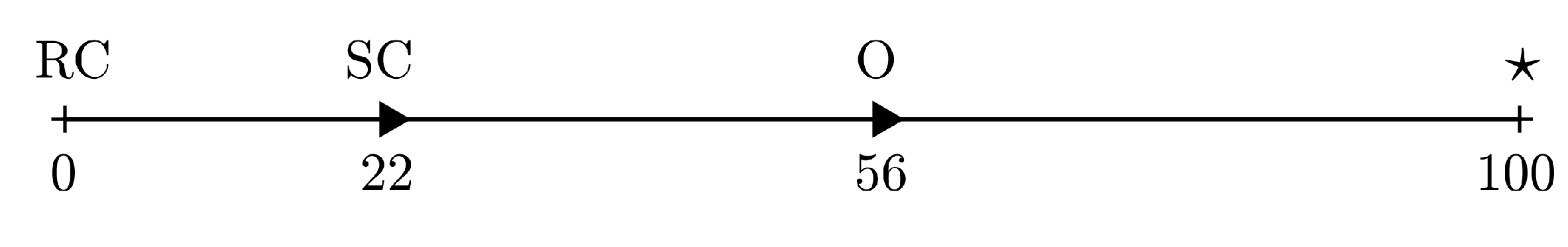
Another way of visualizing this result is to construct a “utopian operational path chart” is presented in Figure 14.

This graphic is constructed by normalizing the performance index between 0 and 100, with 0 being the performance of the Regulatory Control and 100 being the utopian performance. It is possible to see that the Supervisory control was able to move 22 points in the utopian path and the Optimization was able to move 54 points. This is a good way of visualizing the benefit of the implementation of RTO and the potential for improvement of the control and optimization strategies.

5. Conclusions

The present paper describes the development of an RTO strategy for small-scale applications and its implementation to a Debutanizer section of a Natural Gas Processing Unit. The whole methodology is disclosed, including a proposition of a new modeling method for enhancing the effectiveness of the use of sequential-modular models inside an optimization framework and a new method to account for the economic benefit of applications based on optimization frameworks after a period of operation. The developed model proved to be adherent to measured data, which emphasizes its adequacy to be applied for optimization purposes. The implementation of RTO in a closed loop presented not only an economic benefit, but also operational benefits observed from the reduction of variability of the key variables of the process. Moreover, the low computational cost and the great economic benefits indicate the success of the proposed Modular Continuous with Successive Substitution in enhancing the efficiency of sequential-modular simulators in optimization schemes. In addition, it also indicates the potential to spread the application of small-scale RTO to other applications and even to applications where a slow RTO has already been implemented. Finally, RTO showed an increase in operational aspects, as observed by the reduction in variability of the main variables of the system, and in economic aspects, as shown by an increase of 0.64% in profit return when compared with the operation of the regulatory control layer alone.

References

1. Trierweiler, J.O. Real-Time Optimization of Industrial Processes. In Encyclopedia of Systems and Control; Springer: Berlin, Germany, 2014; pp. 1–12. [Google Scholar] [CrossRef]
2. Jang, S.; Joseph, B.; Mukai, H. On-line optimization of constrained multivariable chemical processes. AIChE J. 1987, 33, 26–35. [Google Scholar] [CrossRef]
3. Câmara, M.M.; Quelhas, A.D.; Pinto, J.C. Performance evaluation of real industrial RTO systems. Processes 2016, 4, 44. [Google Scholar] [CrossRef] [Green Version]
4. Müller, D.; Dercks, B.; Nabati, E.; Blazek, M.; Eifert, T.; Schallenberg, J.; Piechottka, U.; Dadhe, K. Real-Time Optimization in the Chemical Processing Industry. Chem. Ing. Tech. 2017, 89, 1464–1470. [Google Scholar] [CrossRef]
5. Quelhas, A.D.; de Jesus, N.J.C.; Pinto, J.C. Common vulnerabilities of RTO implementations in real chemical processes. Can. J. Chem. Eng. 2013, 91, 652–668. [Google Scholar] [CrossRef]
6. Marchetti, A.G.; de Avila Ferreira, T.; Costello, S.; Bonvin, D. Modifier Adaptation as a Feedback Control Scheme. Ind. Eng. Chem. Res. 2020, 59, 2261–2274. [Google Scholar] [CrossRef]
7. Marchetti, A.G.; François, G.; Faulwasser, T.; Bonvin, D. Modifier adaptation for real-time optimization—Methods and applications. Processes 2016, 4, 55. [Google Scholar] [CrossRef] [Green Version]
8. Marlin, T.; Hrymak, A. Real-Time Operations Optimization of Continuous Processes. In AIChE Symp Series CPC V; American Institute of Chemical Engineers: New York, NY, USA, 1997; Volume 93. [Google Scholar]
9. Biegler, L.; Grossmann, I.; Westerberg, A. A note on approximation techniques used for process optimization. Comput. Chem. Eng. 1985, 9, 201–206. [Google Scholar] [CrossRef]
10. Forbes, J.; Marlin, T.; MacGregor, J. Model adequacy requirements for optimizing plant operations. Comput. Chem. Eng. 1994, 18, 497–510. [Google Scholar] [CrossRef]
11. Forbes, J.F.; Marlin, T.E. Model Accuracy for Economic Optimizing Controllers: The Bias Update Case. Ind. Eng. Chem. Res. 1994, 33, 1919–1929. [Google Scholar] [CrossRef]
12. Bhat, S.A.; Saraf, D.N. Steady-State Identification, Gross Error Detection, and Data Reconciliation for Industrial Process Units. Ind. Eng. Chem. Res. 2004, 43, 4323–4336. [Google Scholar] [CrossRef]
13. Rhinehart, R.R. Automated steady and transient state identification in noisy processes. In Proceedings of the 2013 American Control Conference, Washington, DC, USA, 17–19 June 2013; pp. 4477–4493. [Google Scholar] [CrossRef]
14. Øyvind Øksnes Dalheim; Steen, S. A computationally efficient method for identification of steady state in time series data from ship monitoring. J. Ocean. Eng. Sci. 2020, 5, 333–345. [Google Scholar] [CrossRef]
15. Krishnamoorthy, D.; Foss, B.; Skogestad, S. Steady-state real-time optimization using transient measurements. Comput. Chem. Eng. 2018, 115, 34–45. [Google Scholar] [CrossRef]
16. Matias, J.O.; Le Roux, G.A. Real-time Optimization with persistent parameter adaptation using online parameter estimation. J. Process Control 2018, 68, 195–204. [Google Scholar] [CrossRef]
17. Roberts, P.D. An algorithm for steady-state system optimization and parameter estimation. Int. J. Syst. Sci. 1979, 10, 719–734. [Google Scholar] [CrossRef]
18. Chachuat, B.; Marchetti, A.; Bonvin, D. Process optimization via constraints adaptation. J. Process Control 2008, 18, 244–257. [Google Scholar] [CrossRef]
19. Marchetti, A.; Chachuat, B.; Bonvin, D. Modifier-adaptation methodology for real-time optimization. Ind. Eng. Chem. Res. 2009, 48, 6022–6033. [Google Scholar] [CrossRef] [Green Version]
20. de Avila Ferreira, T.; Wuillemin, Z.; Marchetti, A.; Salzmann, C.; Herle, J.V.; Bonvin, D. Real-time optimization of an experimental solid-oxide fuel-cell system. J. Power Sources 2019, 429, 168–179. [Google Scholar] [CrossRef]
21. de Avila Ferreira, T.; Wuillemin, Z.; Faulwasser, T.; Salzmann, C.; herle, J.V.; Bonvin, D. Enforcing optimal operation in solid-oxide fuel-cell systems. Energy 2019, 181, 281–293. [Google Scholar] [CrossRef]
22. Gao, W.; Wenzel, S.; Engell, S. A reliable modifier-adaptation strategy for real-time optimization. Comput. Chem. Eng. 2016, 91, 318–328. [Google Scholar] [CrossRef] [Green Version]
23. Gao, W.; Hernández, R.; Engell, S. A Study of Explorative Moves during Modifier Adaptation with Quadratic Approximation. Processes 2016, 4, 45. [Google Scholar] [CrossRef] [Green Version]
24. Matias, J.; Jäschke, J. Using a neural network for estimating plant gradients in real-time optimization with modifier adaptation. IFAC-PapersOnLine 2019, 52, 808–813. [Google Scholar] [CrossRef]
25. de Avila Ferreira, T.; Shukla, H.A.; Faulwasser, T.; Jones, C.N.; Bonvin, D. Real-Time optimization of Uncertain Process Systems via Modifier Adaptation and Gaussian Processes. In Proceedings of the 2018 European Control Conference (ECC), Limassol, Cyprus, 12–15 June 2018; pp. 465–470. [Google Scholar]
26. del Rio Chanona, E.; Graciano, J.A.; Bradford, E.; Chachuat, B. Modifier-Adaptation Schemes Employing Gaussian Processes and Trust Regions for Real-Time Optimization. IFAC-PapersOnLine 2019, 52, 52–57. [Google Scholar] [CrossRef]
27. del Rio Chanona, E.A.; Petsagkourakis, P.; Bradford, E.; Graciano, J.E.A.; Chachuat, B. Real-time optimization meets Bayesian optimization and derivative-free optimization: A tale of modifier adaptation. Comput. Chem. Eng. 2021, 147, 107249. [Google Scholar] [CrossRef]
28. Darby, M.; Nikolaou, M.; Jones, J.; Nicholson, D. RTO: An Overview and Assessment of Current Practice. J. Process Control 2011, 21, 874–884. [Google Scholar] [CrossRef]
29. Liporace, F.S.; Gomes, M.V.; Katata, A.C.; Zanin, A.C.; Moro, L.F.; Porfírio, C.R. PETROBRAS Experience Implementing Real Time Optimization. In International Symposium on Process Systems Engineering: Part A; de Brito Alves, R.M., do Nascimento, C.A.O., Biscaia, E.C., Eds.; Computer Aided Chemical Engineering; Elsevier: Hoboken, NJ, USA, 2009; Volume 27, pp. 1245–1250. [Google Scholar] [CrossRef]
30. Straus, J.; Skogestad, S. Minimizing the complexity of surrogate models for optimization. In 26th European Symposium on Computer Aided Process Engineering; Kravanja, Z., Bogataj, M., Eds.; Computer Aided Chemical Engineering; Elsevier: Amsterdam, The Netherlands, 2016; Volume 38, pp. 289–294. [Google Scholar] [CrossRef]
31. Berna, T.J.; Locke, M.H.; Westerberg, A.W. A new approach to optimization of chemical processes. AIChE J. 1980, 26, 37–43. [Google Scholar] [CrossRef]
32. Biegler, L. Improved infeasible path optimization for sequential modular simulators—I: The interface. Comput. Chem. Eng. 1985, 9, 245–256. [Google Scholar] [CrossRef]
33. Biegler, L.; Cuthrell, J. Improved infeasible path optimization for sequential modular simulators—II: The optimization algorithm. Comput. Chem. Eng. 1985, 9, 257–267. [Google Scholar] [CrossRef]
34. Gomes, M.V.; Bogle, I.D.L.; Biscaia, E.C.; Odloak, D. Using kriging models for real-time process optimisation. In European Symposium on Computer Aided Process Engineering; Braunschweig, B., Joulia, X., Eds.; Computer Aided Chemical Engineering; Elsevier: Hoboken, NJ, USA, 2008; Volume 25, pp. 361–366. [Google Scholar] [CrossRef]
35. Carpio, R.R.; Giordano, R.C.; Secchi, A.R. Enhanced surrogate assisted framework for constrained global optimization of expensive black-box functions. Comput. Chem. Eng. 2018, 118, 91–102. [Google Scholar] [CrossRef]
36. Udugama, I.A.; Taube, M.A.; Mansouri, S.S.; Kirkpatrick, R.; Gernaey, K.V.; Yu, W.; Young, B.R. A Systematic Methodology for Comprehensive Economic Assessment of Process Control Structures. Ind. Eng. Chem. Res. 2018, 57, 13116–13130. [Google Scholar] [CrossRef] [Green Version]
37. Bauer, M.; Craig, I.K. Economic assessment of advanced process control—A survey and framework. J. Process Control 2008, 18, 2–18. [Google Scholar] [CrossRef]
38. Alkaya, D.; Vasantharajan, S.; Biegler, L.T. Successive quadratic programming: Applications in the process industry Successive Quadratic Programming: Applications in the Process Industry. In Encyclopedia of Optimization; Floudas, C.A., Pardalos, P.M., Eds.; Springer: Boston, MA, USA, 2009; pp. 3853–3866. [Google Scholar]
39. Mochizuki, S.; Saputelli, L.; Kabir, S.; Cramer, R.; Lochmann, M.; Reese, R.; Harms, L.; Sisk, C.; Hite, J.; Escorcia, A. Real Time Optimization: Classification and Assessment. SPE Prod. Oper. 2006, 21, 455–466. [Google Scholar] [CrossRef]
40. Xu, F.; Huang, B.; Akande, S. Performance Assessment of Model Pedictive Control for Variability and Constraint Tuning. Ind. Eng. Chem. Res. 2007, 46, 1208–1219. [Google Scholar] [CrossRef]
41. Campos, M.; Gomes, M.; Souza, A.; Barros, A. Optimisation of natural gas plant—Gains in profitability, stability and energy efficiency. Int. Gas Union World Gas Conf. Pap. 2012, 3, 2089–2120. [Google Scholar]
42. Camolesi, V.J.; Moro, L.L.F.; Zanin, A.C. Implantação de um otimizador em tempo real (RTO) no conversor de uma unidade de craqueamento catalítico. Sba Controle Automação Soc. Bras. Autom. 2008, 19, 128–137. [Google Scholar] [CrossRef]
43. Forbes, J.; Marlin, T. Design cost: A systematic approach to technology selection for model-based real-time optimization systems. Comput. Chem. Eng. 1996, 20, 717–734. [Google Scholar] [CrossRef]
44. Biegler, L.T. Nonlinear Programming; Society for Industrial and Applied Mathematics: Philadelphia, PA, USA, 2010. [Google Scholar] [CrossRef]
45. Biegler, L.T.; Hughes, R.R. Infeasible path optimization with sequential modular simulators. AIChE J. 1982, 28, 994–1002. [Google Scholar] [CrossRef]
46. Niederberger, J.; Gama, M.S.; dos Santos, L.C.; da Silva, J.A.; Vargas, C.E.; Ahón, V.R.R.; Silva, E.P.; de Santana Souza, D.F.; Aquino, C.; Aires, J.S.S. PETROX—PETROBRAS Technology in Process Simulation. In 10th International Symposium on Process Systems Engineering: Part A; de Brito Alves, R.M., do Nascimento, C.A.O., Biscaia, E.C., Eds.; Computer Aided Chemical Engineering; Elsevier: Hoboken, NJ, USA, 2009; Volume 27, pp. 675–680. [Google Scholar] [CrossRef]
47. Cao, S.; Rhinehart, R. An efficient method for on-line identification of steady state. J. Process Control 1995, 5, 363–374. [Google Scholar] [CrossRef]
48. Rod, V.; HanČl, V. Iterative estimation of model parameters when measurements of all variables are subject to error. Comput. Chem. Eng. 1980, 4, 33–38. [Google Scholar] [CrossRef]
49. Gill, P.E.; Murray, W.; Saunders, M.A.; Wright, M.H. User’s Guide for NPSOL 5.0: A Fortran Package for Nonlinear Programming; Technical Report SOL 86-1; University of California: Auckland, CA, USA, 1998; pp. 1–44. [Google Scholar]
50. Ito, E.H.; Secchi, A.R.; Gomes, M.V.; Paiva, C.R. Development of a gas composition soft sensor for distillation columns: A simplified model based and robust approach. In International Symposium on Process Systems Engineering (PSE 2018); Eden, M.R., Ierapetritou, M.G., Towler, G.P., Eds.; Talylor FrancIs; Computer Aided Chemical Engineering; Elsevier: Hoboken, NJ, USA, 2018; Volume 44, pp. 661–666. [Google Scholar] [CrossRef]
51. Cutler, C.R.; Ramaker, B.L. Dynamic matrix control—A computer control algorithm. Jt. Autom. Control Conf. 1979, 17, 72. [Google Scholar] [CrossRef]
52. Rotava, O.; Zanin, A. Multivariable control and real-time optimization—An industrial practical view. Hydrocarb. Process. 2005, 84, 61–71. [Google Scholar]
Figure 1. Schemes of the modeling approaches: (a) Sequential Modular; (b) Modular Continuous; the proposed (c) Modular Continuous with Successive Substitution.
Processes 09 01179 g001
Figure 2. Scheme of the SoraIA architecture.
Processes 09 01179 g002
Figure 3. Simplified process flow diagram of the NGPU. V-03—feed accumulator vessel of the Demethanizer tower (T-01); FV-11/12/13/14—feed flow control valves of T-01; TE-01—turboexpander of T-01; P-05/07—heat exchanger of the cold-box of T-01; P-10—condenser of the Deethanizer tower (T-02); V-04—condenser accumulator vessel of T-02; P-14—condenser air-cooler of the Debutanizer tower (T-03); V-05—condenser accumulator vessel of T-03; P-06/09/13—reboiler heat exchangers of T-01/02/03; FV-21/31—feed flow control valves of T-02/03; P-08/12—feed heat exchanger of T-02/03.
Processes 09 01179 g003
Figure 4. Flow sheet of the process model in PETROX.
Processes 09 01179 g004
Figure 5. Data reconciliation results: (a) condenser temperature of T-03; (b) bottom temperature of T-01; (c) ethane content in LPG stream.
Processes 09 01179 g005
Figure 6. Data reconciliation results: (a) bottom temperature of T-03; (b) top temperature of T-03; (c) pentanes content in LPG stream.
Processes 09 01179 g006
Figure 7. Data reconciliation results: (a) temperature of the control tray of T-03; (b) ratio of the content of propane over butanes in LPG; (c) Reflux flow rate of T-03.
Processes 09 01179 g007
Figure 8. Optimization results: variation of the optimal objective function from the reconciliation solution.
Processes 09 01179 g008
Figure 9. Optimization results: ethane content in LPG deviated from the optimal value before and after the RTO loop closing.
Processes 09 01179 g009
Figure 10. Optimization results: pentanes content in LPG deviated from the optimal value before and after the RTO loop closing.
Processes 09 01179 g010
Figure 11. Optimization results: bottom temperature of T-01 deviated from the optimal value before and after the RTO loop closing.
Processes 09 01179 g011
Figure 12. Optimization results: reflux flow rate of T-03 deviated from the optimal value before and after the RTO loop closing.
Processes 09 01179 g012
Figure 13. Optimization results: recirculation flow rate of T-03 deviated from the optimal value before and after the RTO loop closing.
Processes 09 01179 g013
Figure 14. “Utopian operational path” chart. RC—regulatory control; SC—supervisory control; O—optimization; ⋆ —utopian value.
Processes 09 01179 g014