ICP–MS Analysis of Multi-Elemental Profile of Greek Wines and Their Classification According to Variety, Area and Year of Production

Abstract

Major, minor and trace elements in wines from Greece were determined by inductively coupled plasma–mass spectrometry (ICP–MS). The concentrations of 44 elements (Na, Mg, P, K, Ca, Cu, Co, Cr, Zn, Sn, Fe, Mn, Li, Be, B, V, Sr, Ba, Al, Ag, Ni, As, Sn, Hg, Pb, Sb, Cd, Ti, Ga, Zr, Nb, Pd, Te, La, Sm, Ho, Tm, Yb, W, Os, Au, Tl, Th, U) in 90 white and red wines from six different regions in Greece for two consecutive vinification years, 2017 and 2018, were determined. Results for the elements aforementioned were evaluated by multivariate statistical methods, such as discriminant analysis and cluster analysis, and the wines were discriminated according to wine variety and geographical origin. Due to the specific choice of the analytes for multivariate statistical investigation, a prediction rate by cross-validation of 98% could be achieved. The aim of this study was not only to reveal specific relationships between the wine samples or between the chemical variables in order to classify the wines from different regions and varieties according to their elemental profile (wine authentication), but also to observe the annual fluctuation in the mineral content of the studied wine samples.

1. Introduction

Wine is a complex matrix and, it contains low-level concentrations of mineral elements [1]. Data on mineral elements as probe of origin determination must be carefully interpreted because mineral content in wines depends on many factors that can easily mask vital elemental information [2]. Many of these factors are natural sources (vineyard soil geochemistry), external contamination of the grapevine during growth, contamination through the winemaking process, as well as grape variety, maturity, and climatic conditions [3,4]. Other potential sources that affect mineral content are soil amendments, atmospheric pollution, pesticides, fertilizers, irrigation water, contact materials during transport, vinification and aging processes, enological processing aids, and additives [5,6,7]. For these reasons, wine classification reflects not only the geographical provenance but also anthropogenic factors. Metals are the best-placed descriptors to perform differentiation according to the geographical origin due to the direct relationship with the composition of the soil in which the vine is grown, with Al, Ba, Ca, Cu, Fe, K, Mg, Mn, Na, Sr, and Zn being the most common metal ions determined [8]. Some of these elements, such as Fe, Zn, Cu, Cr, Se, Ca, Co, and Ni, are essential for the human organism in that they form an integral part of one or more enzymes involved in a metabolic or biochemical process [9,10]. Elements are also important for efficient alcoholic fermentation and for the prosthetic metallo-enzyme activation of yeast. In addition, mainly Zn and Fe can contribute to stability and clarity in the wine and its color, and they may affect the organoleptic characteristics of the wine [11]. Depletion of some elements occurs over time, especially during alcoholic fermentation. Precipitation of K and Ca as tartrate salts begins during alcoholic fermentation and continues during the aging period [12]. Alkaline elements, Rb, Li, and Cs, are good indicators of geographical provenance, as they are not included in the group of contaminant elements of wines, while B and Sr are natural elements that originate from their presence in the soil [13]. Mn, Mg, Sr, Ba, and rare-earth elements are also listed as useful elements, although the first two should be considered carefully, as they can be introduced through viticultural practices such as the use of fertilizers and pesticides, while rare-earth element content in wines can increase due to treatment with bentonites [14]. Wine minerals are also useful because of the possibility of toxicological risk, such as Cd and Pb [15,16]. All these factors may markedly change the multi-element composition of the wine, thus precluding their use for authentication purposes [17].

Several studies on this subject have been carried out in most wine producing-countries, such as Argentina [18], Australia [19], Brazil [20,21], Greece [22], Italy [23], Portugal [24], Romania [25], South Africa [26], and Spain [27], indicating that the multi-elemental determination of wines can enable their successful discrimination.

Many multi-element techniques have been employed in elemental analysis in foods, such as atomic emission spectrometry (AES), atomic absorption spectrometry (AAS), inductively coupled plasma–mass spectrometry (ICP–MS), and inductively coupled plasma optical emission spectrometry (ICP–OES) [28]. Inductively coupled plasma–mass spectrometry (ICP–MS) is considered a very potent discriminant technique regarding metal content in wine samples since it provides high detection power due to low detection limits as well as high selectivity and sensitivity [29]. This technique also provides the simultaneous determination of several elements present in low concentrations in the samples [11]. In addition, chemometric analysis (cluster analysis (CA) and discriminant analysis (DA)) was performed to present specific correlations between the chemical variables that characterized the wine samples.

The main goal of this study was to develop a simple, robust, and rapid analytical method with minimum sample pretreatment and low risk of loss of analytes or contamination for the authentication (characterization and differentiation) of Greek wines based on their elemental profile. For this purpose, the direct determination of 44 metals employing ICP–MS instrumentation was carried out for wine samples produced in six different regions of Greece from nine different varieties.

2. Materials and Methods

2.1. Reagents and Materials

Multi-element stock solutions containing 1000 mg/L were used to prepare external standard solutions. TraceSelect concentrated HNO₃ was purchased from Fluka. MilliQ water (Millipore, Burlington, MA, USA) was used for dilutions.

2.2. Wine Samples

A total of 90 wine samples from 9 varieties—white and red—were collected from 6 different regions and various producers in Greece (Figure 1) [4]. The wines were derived from 2 consecutive harvests, 2017 and 2018. An overview of grape varieties, type, and the origin of the Greek wines is given in

Table 1. An overview of the Greek wine samples (number of samples, vinification year, origin, variety, type of wine).

Number of Samples	Year of Production	Origin	Variety	Type
32	17	Arkadia	Moschofilero	white
28	18
2	17	Attika	Syrah	red
2	18
4	17	Attika	Asyrtiko	white
5	18
7	17	Attika	Malagouzia	white
7	18
2	17	Attika	Roditis	white
3	18
6	17	Attika	Savatiano	white
10	18
1	17	Naousa	Syrah	red
1	18
9	17	Naousa	Xinomavro	red
9	18
8	17	Nemea	Agiorgitiko	red
18	18
4	17	Samos	Muscat	white
4	18
15	17	Santorini	Asyrtiko	white
3	18

, while the mineral concentration of each wine sample is given in the Supplementary File.

Table 2. An overview of metal content (mean ± standard deviation) of Greek wine samples for the two consecutive vinifications, 2017 and 2018.

	Vinification Year 2017			Vinification Year 2018
Macro Elements (mg/L)	Mean Concentration ± Standard Deviation			Mean Concentration ± Standard Deviation
K	705	±	265	774	±	264
Ca	81	±	18	85	±	17
P	150	±	47	153	±	37
Na	23	±	19	18	±	13
Mg	87	±	17	103	±	20
Zn	0.52	±	0.23	0.57	±	0,18
Fe	0.86	±	0.56	1.70	±	0.81
Mn	1.3	±	0.43	1.9	±	0.97
B	5.4	±	1.5	5.7	±	1.2
Sr	0.29	±	0.09	0.39	±	0.12
Al	0.57	±	0.39	0.61	±	0.39
Trace elements (ug/L)
Cu	87	±	50	67	±	46
Co	3.8	±	2.1	6.3	±	3.8
Cr	13	±	7.1	14	±	5.1
Se	0.38	±	0.22	0.80	±	0.35
Li	13	±	12	11	±	7.9
Be	0.37	±	0.59	0.86	±	0.77
V	2.1	±	1.5	4.1	±	2.6
Ba	62	±	25	87	±	28
Ag	0.19	±	0.16	2.4	±	0.76
Ni	29	±	14	34	±	14
As	2.1	±	1.6	1.8	±	1.6
Sn	0.02	±	0.01	0.84	±	0.55
Hg	1.1	±	1.0	13	±	2.6
Pb	18	±	14	24	±	14
Sb	0.73	±	0.55	0.37	±	0.42
Cd	0.30	±	0.32	0.40	±	0.27
Ti	16	±	5.9	19	±	8.1
Ga	0.15	±	0.11	0.13	±	0.11
Zr	1.1	±	0.74	2.5	±	2.1
La	1.2	±	1.1	0.43	±	0.26
W	0.15	±	0.08	0.43	±	0.23
Tl	0.25	±	0.14	0.29	±	0.13
Ultra-trace elements (ng/L)
Nb	57	±	45	104	±	57
Pd	92	±	59	195	±	99
Te	40	±	39	107	±	22
Sm	29	±	24	131	±	131
Ho	11	±	8.2	17	±	8.2
Tm	4.4	±	2.7	24	±	14
Yb	44	±	21	101	±	62
Os	67	±	41	230	±	163
Au	61	±	34	258	±	202
Th	41	±	50	170	±	80
U	61	±	41	162	±	102

summarizes the analytical results (mean concentration ± standard deviation) for the whole set of samples. Considering the mean concentrations, the elements were divided into “macro elements” (concentration > 0.1 mg/L), “trace elements” (concentration ranging from 99.9 μg/L to 0.1 μg/L) and “ultra-trace elements” (concentration < 100 ng/L).

2.3. Sample Reparation

Microwave-assisted digestion was used as it is a very effective technique in extracting the metal ions bound in stable complexes. Microwave sample digestion was carried out in a CEM Mars 5 (CEM Microwave Technology, Buckingham, UK) instrument and the samples were digested using the program recommended by the manufacturer.

Table 3. Microwave digestion conditions.

	Power (W)		Ramp Time (min)	Temperature (°C)	Stirrer	Hold Time (min)
Stage	Maximum	%
1	1600	100	2	165	0	0
2	1600	100	3	175	0	5

shows operational parameters for microwave digestion. Digestion of wine samples was carried out in polytetrafluoroethylene (PTFE) vessels, which were previously cleaned in concentrated nitric acid to avoid any kind of contamination. Each time, 2.5 mL of wine sample and 5 mL of HNO₃ were transferred to the vessel, where the acid was added in portions, as the addition of the entire amount at once would cause a loss of the analyte due to the excessively rapid reaction of organic matter in wine and heating [30]. After the digestion step was completed, the digestion vessels were cooled to room temperature. Then, the solutions were transferred to vials and diluted with Millipore water to a final volume of 20 mL.

2.4. ICP–MS Analysis

Multi-element determination was performed on an Agilent 7700 ICP–MS instrument. In accordance with the analytes of interest, the collision/reaction cell was in “He and No gas mode”. For the ICP–MS analysis, the following mass-to-charge ratios (m/z) were recorded: 23Na, 24Mg, 31P, 39K, 44Ca, 63Cu, 59Co, 52Cr, 64Zn, 78Sn, 56Fe, 55Mn, 7Li, 9Be, 11B, 51V, 88Sr, 137Ba, 27Al, 109Ag, 60Ni, 75As, 118Sn, 202Hg, 208Pb, 121Sb, 111Cd, 47Ti, 71Ga, 90Zr, 93Nb, 105Pd, 125Te, 139La, 146Nd, 147Sm, 165Ho, 169Tm, 172Yb, 182W, 189Os, 197Au, 205Tl, 232Th, 238U. Here, 45 Sc (lg/L) was used as an internal standard to correct instrument drift. Two spiked wine samples were prepared with selected elements in order for the method’s accuracy to be accessed through the recovery. The selected metals were Pb, Cd, As, Cr, Ni, Fe, Mn, Zn, Se, Hg, and Sb, cited in

Table 4. Recovery percentage for selected metals in spike dilutions.

Type	Cr	Mn	Fe	Ni	Zn	As	Se	Pb	Cd	Sb	Hg
white	107	103	105	109	114	110	112	104	107	105	111
red	110	92	100	109	115	111	114	105	104	103	106

. The recovery of all selected metals was within the accepted limits of 80–120% according to Table 4. The instrument and accessories were PC-controlled by Mass Hunter software.

2.5. Statistical Analysis

Statistical analysis of the multi-element data was carried out to evaluate the effect of the year of production on mineral composition and the effect of the variety and region of the wine samples on the mineral content. The statistical analysis of the multi-element composition of the wine samples was first performed by one-way analysis of variance (one-way ANOVA) and comparison of means (Tukey’s HSD tests at 95% confidence level). Moreover, a normality test (Anderson Darling test), test for equal variances (Levene test), and a run test were carried out in order to check if the results met the requirements of the one-way ANOVA. Whenever the parametric test assumptions were not verified, a data transformation was attempted with Box–Cox or Johnson transformation and a non-parametric test (Kruskal–Wallis test) was applied. In these cases, comparison of means was not carried out. Correlations between metal concentrations were carried out (Pearson correlations). The data were then processed using multivariate chemometric methods, namely cluster analysis (CA) and discriminant analysis (DA), in order to determine, for each element, the main effect of the region and variety, using the Statistica software package (Statsoft Inc., Tulsa, Version 12, OK, USA), IBM SPSS Statistics 25, SIMCA (Umetrics, version 15.0.2, Umeå, 907 29, Sweden), Minitab 19, and R.

To validate the classification model based on the ICP–MS method, external and internal validation were performed. For classification of the samples regarding variety and area of production, OPLS-DA and O2PLS-DA methods were used. A separate data set (as a test set) from the experimental data set (training set) was used to validate the discrimination ability [31,32]. Training and test sets were randomly generated by keeping in both sets samples from all the groups. Approximately 70% of the overall samples (N = 90) were kept in the training sets and the remaining 30% in the test sets. UV scaling was used throughout this study. The confidence level of parameters was set to 95% and the significance level for distance to the model and Hotelling’s T2 was set to 0.05.

3. Results and Discussion

3.1. Preliminary Classification of Wines According to Elemental Composition

Cluster analysis displays the similarity of objects and classifies them into clusters, so that they are similar within a class but different from those in other classes with respect to the predetermined selection criterion. Hierarchical cluster analysis is the most common approach, and all the data are illustrated by a dendrogram. Cluster analysis is also used to group variables into homogenous and distinct groups. The grouping of the variables by means of cluster analysis helps to identify redundant variables and reduce their number [15]. The HCA was performed after standardizing the input raw data and finding the Euclidean distance measure and Ward’s linkage method. The data were standardized according to the equation:

$$\frac{\mathit{X}-\overline{\mathit{X}}}{\mathit{S}}$$

where $\mathit{X}$: sample;

$\overline{\mathit{X}}$: average;

$S$: standard deviation.

For the vintage year 2017 (Figure 1), the unsupervised clustering led to the formation of four significant clusters:

K1 (K, Tl, Os, Au, Se, Pd, Ba, P, Mg, B, Fe, Sr);

K2 (Ca, Cu, Na, V, Li, Co, Mn, Cr, Ni, Zn, Sn, Te, La, Pb, Sb);

K3 (Tm, Hg, Al, As, Ag, Cd);

K4 (Be, Ga, Zr, Yb, Sm, Ho, Th, U, Ti, Nb, W).

Concerning the vintage year 2018 (Figure 2), the clustering led to the following four significant clusters:

K1 (K, Tl, P, Sn, Mg, Sr, B, Te, Ca, Cu, Cr, Pd, Hg, Ba, Ni, Pb);

K2 (Co, Mn, Os, Cd, Zn, Sb, Se, W, Ti, Nb);

K3 (Li, La, Sm, Ho, Th, Ag);

K4 (Na, Fe, Au, Be, Zr, U, V, Al, As, Tm, Yb, Ga).

Figure 2. Hierarchical dendrogram for 44 chemical variables for the vintage year 2018. The clustering led to the following 4 significant clusters: K1 (K, Tl, P, Sn, Mg, Sr, B, Te, Ca, Cu, Cr, Pd, Hg, Ba, Ni, Pb), K2 (Co, Mn, Os, Cd, Zn, Sb, Se, W, Ti, Nb), K3 (Li, La, Sm, Ho, Th, Ag), and K4 (Na, Fe, Au, Be, Zr, U, V, Al, As, Tm, Yb, Ga).

Figure 2. Hierarchical dendrogram for 44 chemical variables for the vintage year 2018. The clustering led to the following 4 significant clusters: K1 (K, Tl, P, Sn, Mg, Sr, B, Te, Ca, Cu, Cr, Pd, Hg, Ba, Ni, Pb), K2 (Co, Mn, Os, Cd, Zn, Sb, Se, W, Ti, Nb), K3 (Li, La, Sm, Ho, Th, Ag), and K4 (Na, Fe, Au, Be, Zr, U, V, Al, As, Tm, Yb, Ga).

After this grouping, a correlation matrix plot was produced in order to distinguish the relations between the metals. Figure 3 and Figure 4 clearly show the positive (with blue shading) and negative (with red shading) correlation of metals, which corresponds with the clusters that are mentioned above. In particular, suitable forecasting models were created with 95% continuous integration (CI) and a 95% prediction interval (PI), and we selected those that had an average up to 30% R-sq. R-squared (R²) is a statistical measure that represents the proportion of the variance for a dependent variable that is explained by an independent variable or variables in a regression model. Whereas correlation explains the strength of the relationship between an independent and dependent variable, R-squared explains the extent to which the variance of one variable explains the variance of the second variable. Therefore, if the R² of a model is 0.50, then approximately half of the observed variation can be explained by the model’s inputs [33]. Considering Figure 3, it is clearly observed that the maximum correlation results from cluster (K1) are between the metals K, Tl, Mg, P, Fe, and B; from (K2), they are Co, Mn, V, and Na, and from (K4), they are Zr, Ho, Yb, Sm, Th, and U, whereas Figure 4 distinguishes the correlations between the pairs from cluster (K1) Mg with Sr, from cluster (K2) Co, Mn, and Os, from cluster (K3) Li, La, and Sm, and from cluster (K4), Na, Fe, Be, V, Zr, Yb, Au, U, Ga, and Tm.

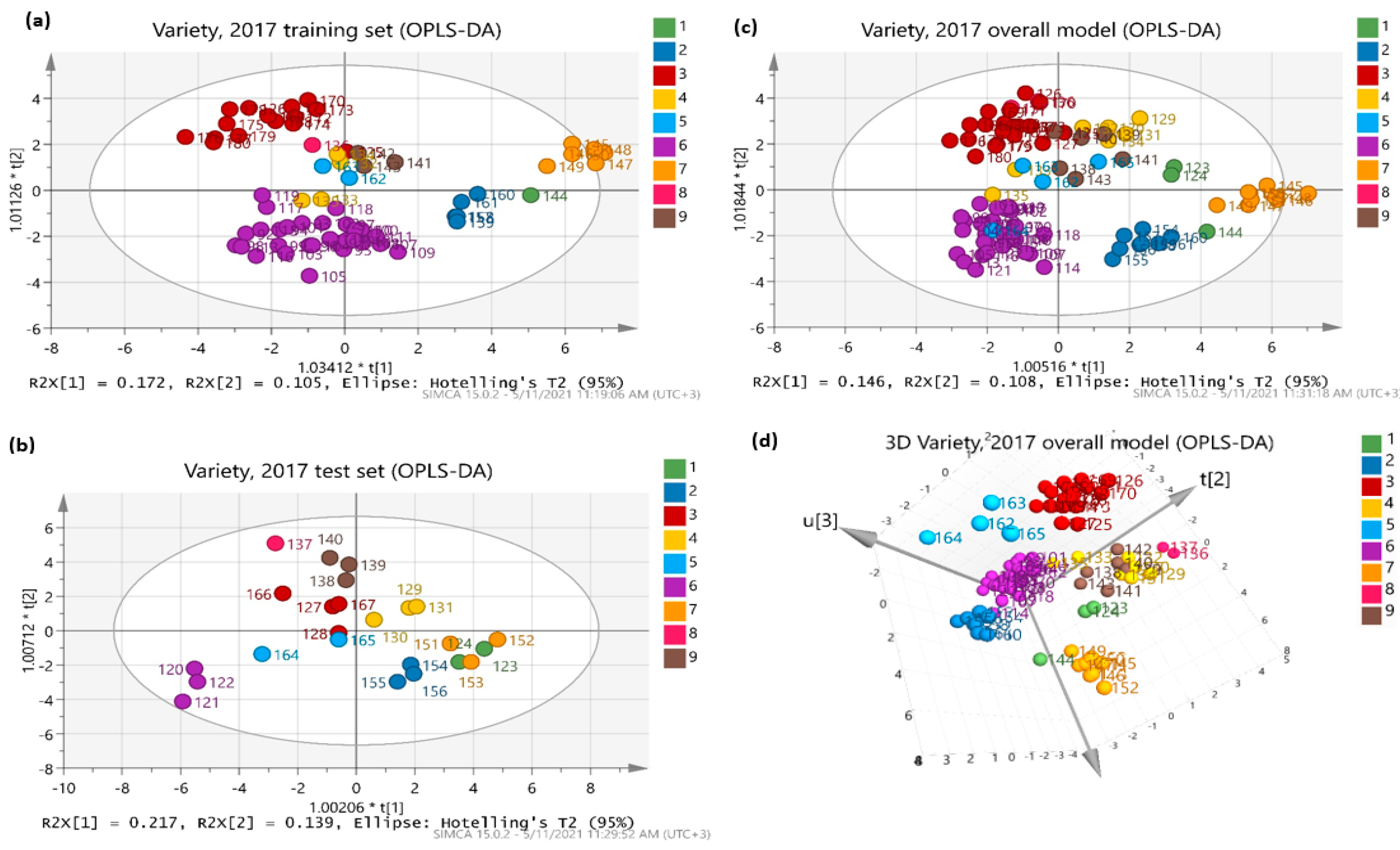
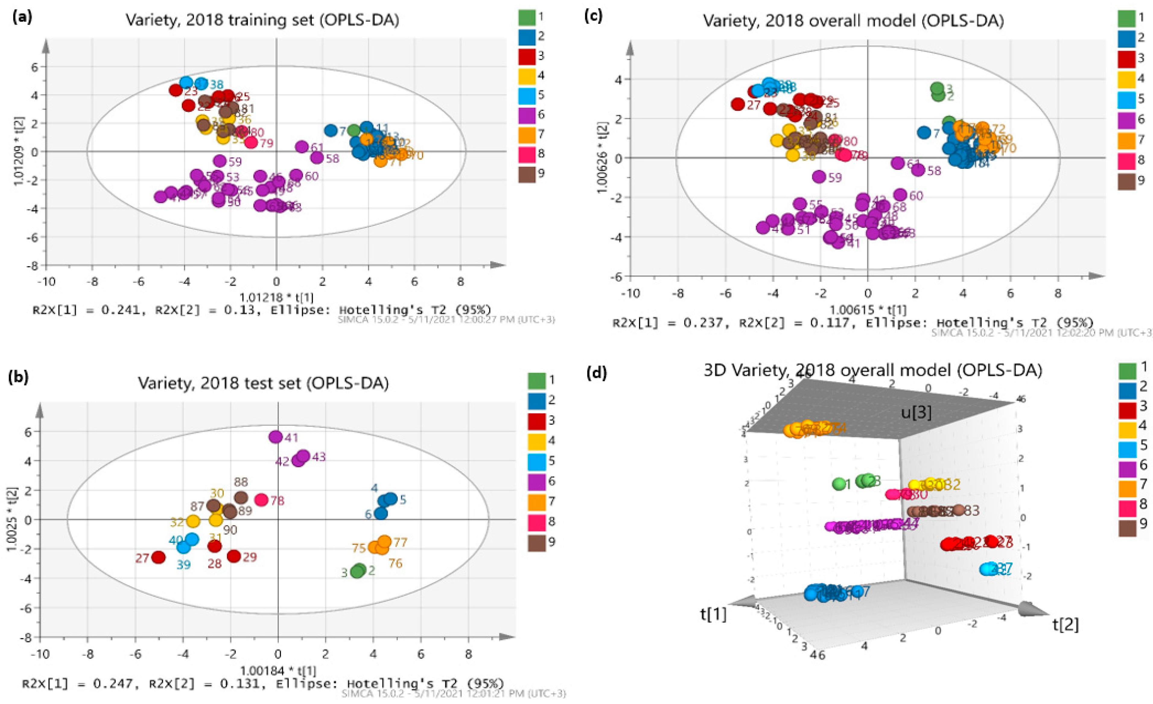
3.2. Classification of Wines According to Their Grape Variety

Aiming to verify if mineral content allows the classification of wines according to their variety, a discriminant analysis was performed. Figure 5 and Figure 6 reflect the discriminating ability of the OPLS-DA model, which can be observed in the scatter plot, showing a reasonably good classification among samples according to the variety of wine. In particular, Agiorgitiko, Asystiko, Malagoyzia, Muscat, Mosxofilero, Xinomavro, Roditis, Savatiano, and Syrah are clearly separated, with a proportion of 97.78% and 96.67% for both harvest years, respectively.

Table 5. Misclassification tables produced for the OPLS-DA models of the wine samples of 2017 classified regarding variety, where (a) training set, (b) test set, (c) overall model.

(a) Variety, 2017 Training Set	Samples	Correct	1	2	3	4	5	6	7	8	9
1 Syrah	1	0%	0	0	0	0	0	0	1	0	0
2 Agioritiko	5	100%	0	5	0	0	0	0	0	0	0
3 Asyrtiko	15	100%	0	0	15	0	0	0	0	0	0
4 Malagouzia	4	75%	0	0	0	3	0	1	0	0	0
5 Muscat	2	100%	0	0	0	0	2	0	0	0	0
6 Moschofilero	29	100%	0	0	0	0	0	29	0	0	0
7 Xinomavro	6	100%	0	0	0	0	0	0	6	0	0
8 Roditis	1	100%	0	0	0	0	0	0	0	1	0
9 Savatiano	3	100%	0	0	0	0	0	0	0	0	3
Total	66	96.97%
(b) Variety, 2017 Test Set	Samples	Correct	1	2	3	4	5	6	7	8	9
1 Syrah	2	100%	2	0	0	0	0	0	0	0	0
2 Agioritiko	3	100%	0	3	0	0	0	0	0	0	0
3 Asyrtiko	4	100%	0	0	4	0	0	0	0	0	0
4 Malagouzia	3	100%	0	0	0	3	0	0	0	0	0
5 Muscat	2	100%	0	0	0	0	2	0	0	0	0
6 Moschofilero	3	100%	0	0	0	0	0	3	0	0	0
7 Xinomavro	3	100%	0	0	0	0	0	0	3	0	0
8 Roditis	1	100%	0	0	0	0	0	0	0	1	0
9 Savatiano	3	100%	0	0	0	0	0	0	0	0	3
Total	24	100%
(c) Variety, 2017 Overall Model	Samples	Correct	1	2	3	4	5	6	7	8	9
1 Syrah	3	66.67%	2	0	0	0	0	0	1	0	0
2 Agioritiko	8	100%	0	8	0	0	0	0	0	0	0
3 Asyrtiko	19	100%	0	0	19	0	0	0	0	0	0
4 Malagouzia	7	85.71%	0	0	0	6	0	1	0	0	0
5 Muscat	4	100%	0	0	0	0	4	0	0	0	0
6 Moschofilero	32	100%	0	0	0	0	0	32	0	0	0
7 Xinomavro	9	100%	0	0	0	0	0	0	9	0	0
8 Roditis	2	100%	0	0	0	0	0	0	0	2	0
9 Savatiano	6	100%	0	0	0	0	0	0	0	0	6
Total	90	97.78%

and

Table 6. Misclassification tables produced for the OPLS-DA models of the wine samples of 2018 classified regarding variety, where (a) training set, (b) test set, (c) overall model.

(a) Variety, 2018 Training Set	Samples	Correct	1	2	3	4	5	6	7	8	9
1 Syrah	1	0%	0	0	0	0	0	0	1	0	0
2 Agioritiko	15	100%	0	15	0	0	0	0	0	0	0
3 Asyrtiko	5	100%	0	0	5	0	0	0	0	0	0
4 Malagouzia	4	0%	0	0	0	0	0	2	0	0	2
5 Muscat	2	0%	0	0	2	0	0	0	0	0	0
6 Moschofilero	25	92%	0	2	0	0	0	23	0	0	0
7 Xinomavro	6	100%	0	0	0	0	0	0	6	0	0
8 Roditis	2	0%	0	0	0	0	0	2	0	0	0
9 Savatiano	6	0%	0	0	4	0	0	2	0	0	0
Total	66	74.24%
(b)Variety, 2018 Test Set	Samples	Correct	1	2	3	4	5	6	7	8	9
1 Syrah	2	100%	2	0	0	0	0	0	0	0	0
2 Agioritiko	3	100%	0	3	0	0	0	0	0	0	0
3 Asyrtiko	3	100%	0	0	3	0	0	0	0	0	0
4 Malagouzia	3	100%	0	0	0	3	0	0	0	0	0
5 Muscat	2	100%	0	0	0	0	2	0	0	0	0
6 Moschofilero	3	100%	0	0	0	0	0	3	0	0	0
7 Xinomavro	3	100%	0	0	0	0	0	0	3	0	0
8 Roditis	1	100%	0	0	0	0	0	0	0	1	0
9 Savatiano	4	100%	0	0	0	0	0	0	0	0	4
Total	24	100%
(c) Variety, 2018 Overall Model	Samples	Correct	1	2	3	4	5	6	7	8	9
1 Syrah	3	66.67%	2	0	0	0	0	0	1	0	0
2 Agioritiko	18	100%	0	18	0	0	0	0	0	0	0
3 Asyrtiko	8	100%	0	0	8	0	0	0	0	0	0
4 Malagouzia	7	71.43%	0	0	0	5	0	0	0	0	2
5 Muscat	4	100%	0	0	0	0	4	0	0	0	0
6 Moschofilero	28	100%	0	0	0	0	0	28	0	0	0
7 Xinomavro	9	100%	0	0	0	0	0	0	9	0	0
8 Roditis	3	100%	0	0	0	0	0	0	0	3	0
9 Savatiano	10	100%	0	0	0	0	0	0	0	0	10
Total	90	96.67%

summarize all the misclassified observations and indicate the predicted groups. The results obtained with this canonical analysis show that, using the elemental composition of wines, it is possible to discriminate among these wines considering the grape variety, as the proportion of the correctly classified chemical variables is incomparable with the misclassified.

Analytically, by observing the results of Table 6, it could be said that three samples (1 from Syrah and 2 from Malagouzia groups) are wrongly classified; thus, they are responsible for lowering the successful classification of the overall model (Table 6c) to 96.67%. In future, more samples from these two varieties and provinces are considered important to be added to the model, as the more samples each group contains, the better classification is obtained. As can be seen in Table 6a, in the training set, several samples were misclassified, but when they were mixed with the test set, the overall model was improved.

The same pattern can be observed in Table 5. Overall, two samples (1 from Syrah and 1 from Malagouzia groups) are wrongly classified; thus, they are responsible for lowering the successful classification of the overall model (Table 5c) to 97.78%. The R2X(cum), R2Y(cum), and Q2(cum) scores of classifications for the wine samples between 2017 to 2018 regarding variety are presented in

Table 7. The R2X(cum), R2Y(cum), and Q2(cum) scores of classifications for the wine samples between 2017 to 2018 regarding variety by OPLS-DA.

Vintage Year	Set	N	R2X(cum)	R2Y(cum)	Q2(cum)
2017	training	66	0.682	0.676	0.584
	test	24	0.833	0.889	0.600
	overall	90	0.770	0.711	0.595
2018	training	66	0.804	0.798	0.525
	test	24	0.814	0.863	0.517
	overall	90	0.748	0.687	0.598

. It can be observed that the values of R² and Q2 indicated that the model had very good fitness and prediction ability as both R² and Q2 > 0.5, and the difference between R2Xcum and Q2cum was less than 0.2–0.3, highlighting the importance of the models. The result shows that the classification model is feasible and successful regarding variety.

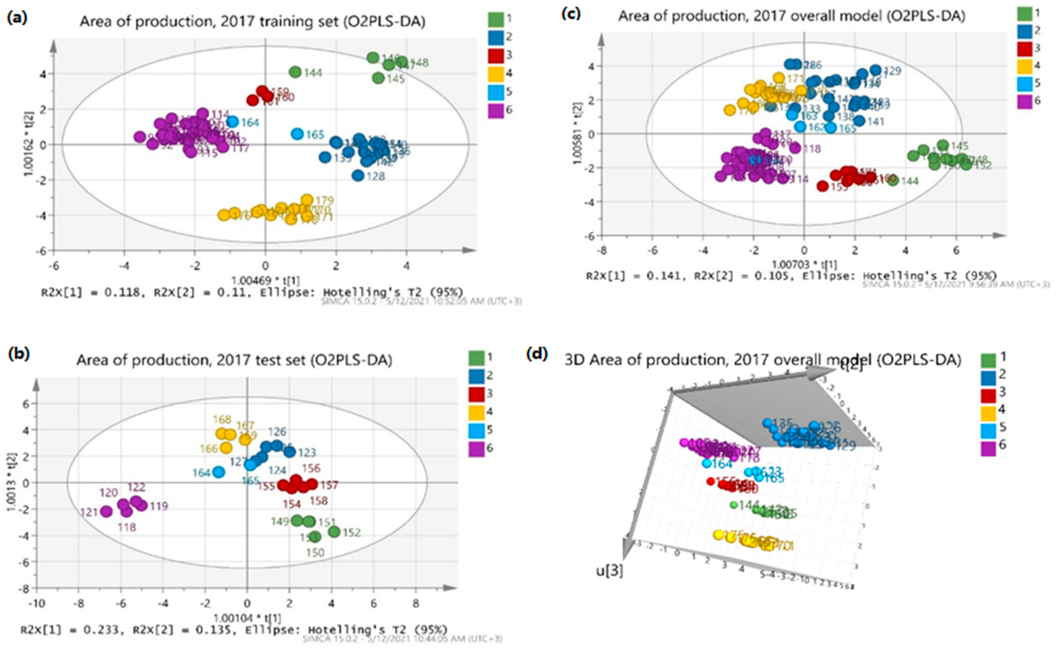
3.3. Classification of Wines According to Their Area of Production

Taking into consideration that the mineral composition of wines reflects the elemental composition of the vineyard and is a consequence of the wine’s origin, multi-elemental analysis is an important tool in the wine industry. Several studies have been performed to find chemical markers that allow the traceability of wines [34,35].

The O2PLS-DA results of the training set displayed excellent goodness of fit (R2Ycum) and predictability (Q2cum) for the discrimination of the samples regarding the six areas of production, as shown in

Table 8. Misclassification tables produced for the O2PLS-DA models of the wine samples of 2017 classified regarding area of production, where (a) training set, (b) test set, (c) overall model.

(a) Area of production, 2017 Training Set	Samples	Correct	1	2	3	4	5	6
1 Naousa	5	100%	5	0	0	0	0	0
2 Attika	16	100%	0	16	0	0	0	0
3 Nemea	3	100%	0	0	3	0	0	0
4 Santorini	11	100%	0	0	0	11	0	0
5 Samos	2	100%	0	0	0	0	2	0
6 Arkadia	27	100%	0	0	0	0	0	27
Total	64	100%
(b)Area of production, 2017 Test Set	Samples	Correct	1	2	3	4	5	6
1 Naousa	5	100%	5	0	0	0	0	0
2 Attika	5	100%	0	5	0	0	0	0
3 Nemea	5	100%	0	0	5	0	0	0
4 Santorini	4	100%	0	0	0	4	0	0
5 Samos	2	100%	0	0	0	0	2	0
6 Arkadia	5	100%	0	0	0	0	0	5
Total	26	100%
(c) Area of production, 2017 Overall Model	Samples	Correct	1	2	3	4	5	6
1 Naousa	10	100%	10	0	0	0	0	0
2 Attika	21	100%	0	21	0	0	0	0
3 Nemea	8	100%	0	0	8	0	0	0
4 Santorini	15	100%	0	0	0	15	0	0
5 Samos	4	100%	0	0	0	0	4	0
6 Arkadia	32	100%	0	0	0	0	0	32
Total	90	100%

and

Table 9. Misclassification tables produced for the O2PLS-DA models of the wine samples of 2018 classified regarding area of production, where (a) training set, (b) test set, (c) overall model.

(a) Area of production, 2018 Training Set	Samples	Correct	1	2	3	4	5	6
1 Naousa	5	100%	5	0	0	0	0	0
2 Attika	21	100%	0	21	0	0	0	0
3 Nemea	14	100%	0	0	14	0	0	0
4 Santorini	1	100%	0	0	0	1	0	0
5 Samos	2	100%	0	0	0	0	2	0
6 Arkadia	23	100%	0	0	0	0	0	23
Total	66	100%
(b)Area of production, 2018 Test Set	Samples	Correct	1	2	3	4	5	6
1 Naousa	5	100%	5	0	0	0	0	0
2 Attika	6	100%	0	6	0	0	0	0
3 Nemea	4	100%	0	0	4	0	0	0
4 Santorini	2	100%	0	0	0	2	0	0
5 Samos	2	100%	0	0	0	0	2	0
6 Arkadia	5	100%	0	0	0	0	0	5
Total	24	100%
(c)Area of production, 2018 Overall Model	Samples	Correct	1	2	3	4	5	6
1 Naousa	10	100%	10	0	0	0	0	0
2 Attika	27	100%	0	27	0	0	0	0
3 Nemea	18	100%	0	0	18	0	0	0
4 Santorini	3	100%	0	0	0	3	0	0
5 Samos	4	100%	0	0	0	0	4	0
6 Arkadia	28	100%	0	0	0	0	0	28
Total	90	100%

. Then, the test set was imported into the training set to test the distribution of all the samples together. Therefore, the overall model was obtained and the coefficients R² and Q2 (

Table 10. The R2X(cum), R2Y(cum), and Q2(cum) scores of classifications for the wine samples between 2017 to 2018 regarding area of production by O2PLS-DA.

Vintage Year	Set	N	R2X(cum)	R2Y(cum)	Q2(cum)
2017	training	64	0.766	0.875	0.719
	test	26	0.867	0.951	0.765
	overall	90	0.781	0.844	0.642
2018	training	66	0.632	0.811	0.570
	test	24	0.743	0.898	0.702
	overall	90	0.736	0.818	0.622

) as well as the % of correct classification (Table 8 and Table 9) were still very good. All the test set samples could be classified into the correct area of production group. No outlier observations (in the area outside of an ellipse with a 95% confidence interval for Hotelling’s T2 on the score plots) in Figure 7 and Figure 8 were observed and this explains the 100% excellent classification of the samples in Table 8 and Table 9. From Table 10, it can be observed that the values of R² and Q2 indicated that the model had very good fitness and prediction ability as both R² and Q2 > 0.5, and the difference between R2Xcum and Q2cum was less than 0.2–0.3, highlighting the importance of the models. The result shows that the geographical classification model is feasible and successful.

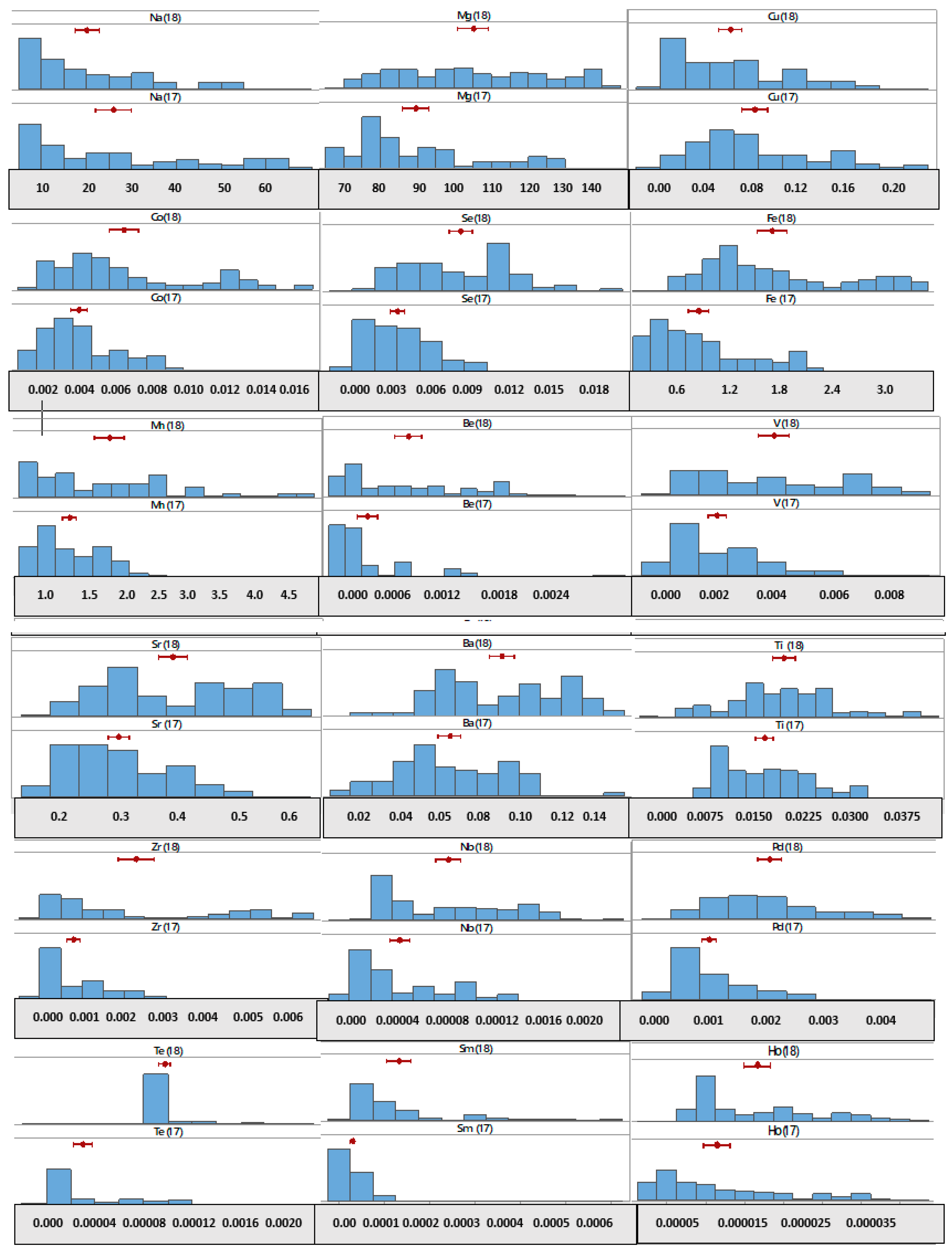
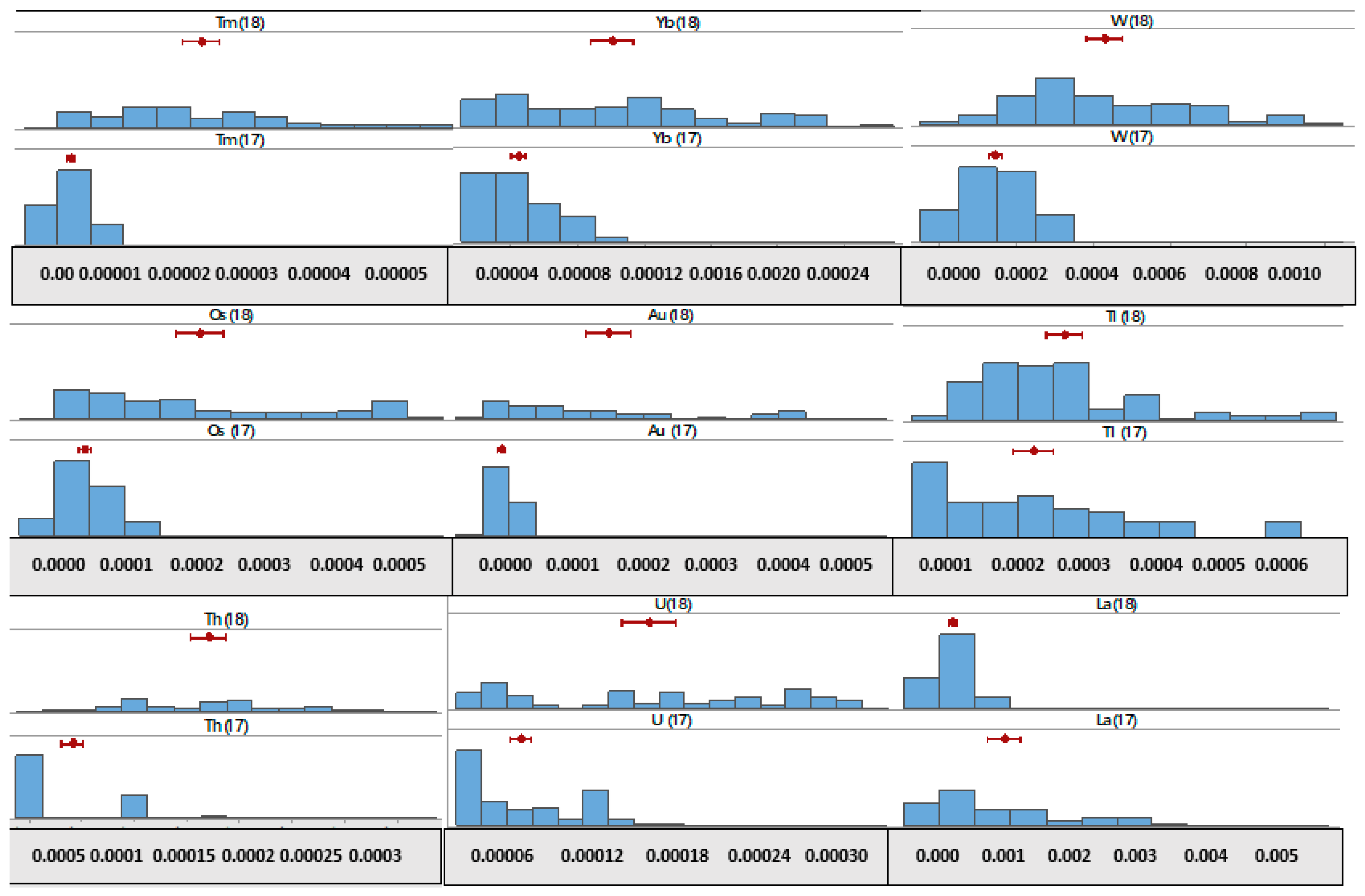
3.4. Annual Fluctuation in Mineral Content

Analysis of measurement results reveals how seasonal changes over the years influence the concentration of analytes. After a t-test analysis, there was not any significant variation between K (p = 0.079), Ca (p = 0.113), P (p = 0.679), Cr (p = 0.199), Zn (p = 0.104), Li (p = 0.121), B (p = 0.084), and Ga (p = 0.124). However, other elements differed statistically, particularly some rare-earth elements that indicate the minimum level of significance (p < 0.001), such as U, Th, Au, Os, W, Pd, Yb, Tm, Ho, Sm, La, Te, Pd, Nb, Zr, Ba, Sr, V, Be, Mn, Fe, Se and Co, Na (p = 0.020), Mg (p = 0.001), Cu (p = 0.005), Ti (p = 0.008), and Tl (p = 0.026). As the graphical depiction shows (Figure 9), most of the aforementioned metals displayed higher concentration levels in wine samples from vintage 2018, with the exception of Na and La, which had lower concentration levels in the same harvest year compared with the concentration levels in harvest 2017.

These statistical differences in the concentration levels of metals in the wine samples can be attributed to the significant rainfall in the early summer of the year 2018. It is widely known that wine water status depends on the climate (rainfall and potential evapotranspiration), soil (water holding capacity), and training system (canopy architecture and leaf area). Wine water uptake conditions are a key factor in understanding the effect of the terroir on grape quality potential, because the main terroir factors are involved and interact (climate, soil, grapevine). The proportions of mineral nutrients in the finished wine bear only a complex, indirect, and distant relationship with the geological minerals in the vineyard. This is why it has proven so difficult to find a reliable chemical means of using the inorganic constituents of a wine to detect the annual adulteration of the multi-element profile [36,37]. Many surveys have studied the impact of environmental factors and climatic changes on wine physiology [38]. Others have pointed out the influence of vineyard on the mineral composition of the wine [39]. However, it is very difficult to assess the joint effect of all the different geographic variables (soils, climate, microclimate, slope, etc.) that make up a vineyard; the effects caused by these parameters on wine have been independently reported.

From the comparison of results of the wine samples from the 2017 and 2018 vintages, it could be concluded that the element composition of wine is not dependent only on the year of production but on many other factors that must be studied. Of course, this result must be confirmed with a larger number of samples and other vintages so as to gain a more consolidated view.

4. Conclusions

Mineral content in wines is of great importance for authenticity purposes and quality control. Minerals can influence a wine’s taste and quality, stability, and the toxicological risks associated with wine consumption, since some of them are regulated by law. In this study, an ICP–MS procedure enabled the quantification of 44 mineral elements from 90 wine samples from six different regions in Greece in two consecutive harvests. The statistical analysis of data obtained by ICP–MS has shown that a compensatory differentiation of the wine samples can be achieved concerning their multi-element composition from different varieties and cultivated regions. Therefore, the presented results suggest that the multi-element composition of the provenance also has potentialities to be used as a fingerprint of the origin of wines from the Greek wine district. Nevertheless, more wines from the same and/or other wine districts must be analyzed so as to consolidate this conclusion. A further analysis of vinification processes and fertilization practices in wine samples could be a useful tool for further differentiation concerning the provenance. Moreover, studies on the variability of soil properties could provide more details with which to understand the mineral characteristics of wines.

References

1. Pasvanka, K.; Tzachristas, A.; Proestos, C. Quality Tools in Wine Traceability and Authenticity. In Quality Control in the Beverage Industry; Academic Press: New York, NY, USA, 2019; pp. 289–334. [Google Scholar] [CrossRef]
2. Catarino, S.; Curvelo-Garcia, A.S.; Bruno de Sousa, R. Contaminant elements in wines: A review. Ciênc. Téc. Vitiv. 2008, 23, 3–19. [Google Scholar]
3. Likar, M.; Vogel-Mikuš, K.; Potisek, M.; Hančević, K.; Radić, T.; Nečemer, M.; Regvar, M. Importance of soil and vineyard management in the determination of grapevine mineral composition. Sci. Total Environ. 2015, 505, 724–731. [Google Scholar] [CrossRef]
4. Pasvanka, K.; Tzachristas, A.; Kostakis, M.; Thomaidis, N.; Proestos, C. Geographic characterization of Greek wine by inductively coupled plasma–mass spectrometry macroelemental analysis. Anal. Lett. 2019, 52, 2741–2750. [Google Scholar] [CrossRef]
5. Médina, B.; Augagneur, S.; Barbaste, M.; Grousset, F.E.; Buat-Ménard, P. Influence of atmospheric pollution on the lead content of wines. Food Addit. Contam. 2000, 6, 435–445. [Google Scholar] [CrossRef] [PubMed]
6. Nicolini, G.; Larcher, R.; Pangrazzi, P.; Bontempo, L. Changes in the contents of micro- and trace-elements in wine due to winemaking treatments. Vitis 2004, 43, 41–45. [Google Scholar]
7. Volpe, M.G.; La Cara, F.; Volpe, F.; De Mattia, A.; Serino, V.; Petitto, F.; Zavalloni, C.; Limone, F.; Pellechia, R.; De Prisco, P.P. Heavy metal uptake in the enological food chain. Food Chem. 2009, 117, 553–560. [Google Scholar] [CrossRef]
8. Moreno, I.M.; González-Weller, D.; Gutierrez, V.; Marino, M.; Cameán, A.M.; González, A.G.; Hardisson, A. Determination of Al, Ba, Ca, Cu, Fe, K, Mg, Mn, Na, Sr and Zn in red wine samples by inductively coupled plasma optical emission spectroscopy: Evaluation of preliminary sample treatments. Microchem. J. 2008, 88, 56–61. [Google Scholar] [CrossRef]
9. Pan, X.-D.; Tang, J.; Chen, Q.; Wu, P.-G.; Han, J.-L. Evaluation of direct sampling method for trace elements analysis in Chinese rice wine by ICP-OES. Eur. Food Res. Technol. 2013, 236, 531–535. [Google Scholar] [CrossRef]
10. Catarino, S.; Curvelo-Garcia, A.S. Composição mineral do vinho–Ocorrência de metais contaminantes. In Química Enológicamétodos Analíticos; Publindústria, 2015; Volume 1, pp. 237–273. Available online: https://www.researchgate.net/profile/Sofia-Catarino/publication/259649335_Composicao_mineral_do_vinho_-_Ocorrencia_de_metais_contaminantes/links/02e7e52f563dc36d74000000/Composicao-mineral-do-vinho-Ocorrencia-de-metais-contaminantes.pdf (accessed on 20 July 2021).
11. Pérez-Álvarez, E.P.; García, P.; Barrulas, R.; Dias, C.; Cabrita, M.J.; Garde-Cerdán, T. Classification of wines according to several factors by ICP-MS multi-element analysis. Food Chem. 2019, 270, 273–280. [Google Scholar] [CrossRef] [PubMed]
12. Catarino, S.; Madeira, M.; Monteiro, F.; Caldeira, I.; Bruno de Sousa, R.; Curvelo-Garcia, A. Mineral Composition through Soil-Wine System of Portuguese Vineyards and Its Potential for Wine Traceability. Beverages 2018, 4, 85. [Google Scholar] [CrossRef] [Green Version]
13. Paneque, P.; Morales, M.L.; Burgos, P.; Ponce, L.; Callejón, R.M. Elemental characterisation of Andalusian wine vinegars with protected designation of origin by ICP-OES and chemometric approach. Food Control 2017, 75, 203–210. [Google Scholar] [CrossRef]
14. Catarino, S.; Madeira, M.; Monteiro, F.; Rocha, F.; Curvelo-Garcia, A.S.; Bruno de Sousa, R. Effect of bentonite characteristics on the elemental composition of wine. J. Agric. Food Chem. 2008, 56, 158–165. [Google Scholar] [CrossRef] [PubMed] [Green Version]
15. Kruzlicova, D.; Fiket, Ž.; Kniewald, G. Classification of Croatian wine varieties using multivariate analysis of data obtained by high resolution ICP-MS analysis. Food Res. Int. 2013, 54, 621–626. [Google Scholar] [CrossRef]
16. Lara, R.; Cerutti, S.; Salonia, J.A.; Olsina, R.A.; Martinez, L.D. Trace element determination of Argentine wines using ETAAS and USN-ICP-OES. Food Chem. Toxicol. 2005, 43, 293–297. [Google Scholar] [CrossRef] [PubMed]
17. Almeida, C.M.R.; Vasconcelos, M.T.S. Multielement composition of wines and their precursors including provenance soil and their potentialities as fingerprints of wine origin. J. Agric. Food Chem. 2003, 51, 4788–4798. [Google Scholar] [CrossRef]
18. Fabani, M.P.; Toro, M.E.; Vazquez, F.; Diaz, M.P.; Wunderlin, D.A. Differential absorption of metals from soil to diverse vine varieties from the Valley of Tulum (Argentina): Consequences to evaluate wine provenance. J. Agric. Food Chem. 2009, 57, 7409–7416. [Google Scholar] [CrossRef]
19. Wilkes, E.; Day, M.; Herderich, M.; Johnson, D. AWRI reports: In vino veritas-investigating technologies to fight wine fraud. Wine Vitic. J. 2016, 31, 36. [Google Scholar]
20. Dutra, S.V.; Adami, L.; Marcon, A.R.; Carnieli, G.J.; Roani, C.A.; Spinelli, F.R.; Vanderlinde, R. Determination of the geographical origin of Brazilian wines by isotope and mineral analysis. Anal. Bioanal. Chem. 2011, 401, 1571. [Google Scholar] [CrossRef]
21. Maciel, J.V.; Souza, M.M.; Silva, L.O.; Dias, D. Direct determination of Zn, Cd, Pb and Cu in wine by differential pulse anodic stripping voltammetry. Beverages 2019, 5, 6. [Google Scholar] [CrossRef] [Green Version]
22. Bimpilas, A.; Tsimogiannis, D.; Balta-Brouma, K.; Lymperopoulou, T.; Oreopoulou, V. Evolution of phenolic compounds and metal content of wine during alcoholic fermentation and storage. Food Chem. 2015, 178, 164–171. [Google Scholar] [CrossRef]
23. D’Antone, C.; Punturo, R.; Vaccaro, C. Rare earth elements distribution in grapevine varieties grown on volcanic soils: An example from Mount Etna (Sicily, Italy). Environ. Monit. Assess. 2017, 189, 160. [Google Scholar] [CrossRef]
24. Rodrigues, S.M.; Otero, M.; Alves, A.A.; Coimbra, J.; Coimbra, M.A.; Pereira, E.; Duarte, A.C. Elemental analysis for categorization of wines and authentication of their certified brand of origin. J. Food Compos. Anal. 2011, 24, 548–562. [Google Scholar] [CrossRef]
25. Dinca, O.R.; Ionete, R.E.; Costinel, D.; Geana, I.E.; Popescu, R.; Stefanescu, I.; Radu, G.L. Regional and vintage discrimination of Romanian wines based on elemental and isotopic fingerprinting. Food Anal. Methods 2016, 9, 2406–2417. [Google Scholar] [CrossRef]
26. Coetzee, P.P.; Van Jaarsveld, F.P.; Vanhaecke, F. Intraregional classification of wine via ICP-MS elemental fingerprinting. Food Chem. 2014, 164, 485–492. [Google Scholar] [CrossRef] [PubMed]
27. Bravo, S.; Amorós, J.A.; Pérez-De-Los-Reyes, C.; García, F.J.; Moreno, M.M.; Sánchez-Ormeño, M.; Higueras, P. Influence of the soil pH in the uptake and bioaccumulation of heavy metals (Fe, Zn, Cu, Pb and Mn) and other elements (Ca, K, Al, Sr and Ba) in vine leaves, Castilla-La Mancha (Spain). J. Geochem. Explor. 2017, 174, 79–83. [Google Scholar] [CrossRef]
28. Płotka-Wasylka, J.; Frankowski, M.; Simeonov, V.; Polkowska, Ż.; Namieśnik, J. Determination of metals content in wine samples by inductively coupled plasma-mass spectrometry. Molecules 2018, 23, 2886. [Google Scholar] [CrossRef] [Green Version]
29. Soares, F.; Anzanello, M.J.; Fogliatto, F.S.; Marcelo, M.C.; Ferrão, M.F.; Manfroi, V.; Pozebon, D. Element selection and concentration analysis for classifying South America wine samples according to the country of origin. Comput. Electron. Agric. 2018, 150, 33–40. [Google Scholar] [CrossRef]
30. Zioła-Frankowska, A.; Frankowski, M. Determination of metals and metalloids in wine using inductively coupled plasma optical emission spectrometry and mini-torch. Food Anal. Methods 2016, 10, 180–190. [Google Scholar] [CrossRef] [Green Version]
31. Tarapoulouzi, M.; Theocharis, C.R. Discrimination of Cheddar and Kefalotyri Cheese Samples: Analysis by Chemometrics of Proton-NMR and FTIR Spectra. J. Agric. Sci. Technol. 2019, 9, 347–355. [Google Scholar] [CrossRef]
32. Zhang, J.; Chen, H.; Fan, C.; Gao, S.; Zhang, Z.; Bo, L. Classification of the botanical and geographical origins of Chinese honey based on 1H NMR profile with chemometrics. Food Res. Int. 2020, 137, 109714. [Google Scholar] [CrossRef]
33. Gelman, A.; Goodrich, B.; Gabry, J.; Vehtari, A. R-squared for Bayesian regression models. Am. Stat. 2019, 73, 307–309. [Google Scholar] [CrossRef]
34. Geana, I.; Iordache, A.; Ionete, R.; Marinescu, A.; Ranca, A.; Culea, M. Geographical origin identification of Romanian wines by ICP-MS elemental analysis. Food Chem. 2013, 138, 1125–1134. [Google Scholar] [CrossRef] [PubMed]
35. Sen, I.; Tokatli, F. Characterization and classification of Turkish wines based on elemental composition. Am. J. Enol. Vitic. 2014, 65, 134–142. [Google Scholar] [CrossRef] [Green Version]
36. Galani-Nikolakaki, S.M.; Kallithrakas-Kontos, N.G. Elemental content of wines. In Mineral Components in Foods; CRC Press: Boca Raton, FL, USA, 2006; pp. 323–344. [Google Scholar]
37. Maltman, A. Minerality in wine: A geological perspective. J. Wine Res. 2013, 24, 169–181. [Google Scholar] [CrossRef] [Green Version]
38. Pons, A.; Allamy, L.; Schüttler, A.; Rauhut, D.; Thibon, C.; Darriet, P. What is the expected impact of climate change on wine aroma compounds and their precursors in grape? OENO One 2017, 51, 141–146. [Google Scholar] [CrossRef] [Green Version]
39. Rodrigues, H.; Sáenz-Navajas, M.P.; Franco-Luesma, E.; Valentin, D.; Fernández-Zurbano, P.; Ferreira, V.; Ballester, J. Sensory and chemical drivers of wine minerality aroma: An application to Chablis wines. Food Chem. 2017, 230, 553–562. [Google Scholar] [CrossRef] [PubMed] [Green Version]
Figure 1. Hierarchical dendrogram for 44 chemical variables for the vintage year 2017. The clustering led to the following 4 significant clusters: K1 (K, Tl, Os, Au, Se, Pd, Ba, P, Mg, B, Fe, Sr), K2 (Ca, Cu, Na, V, Li, Co, Mn, Cr, Ni, Zn, Sn, Te, La, Pb, Sb), K3 (Tm, Hg, Al, As, Ag, Cd), and K4 (Be, Ga, Zr, Yb, Sm, Ho, Th, U, Ti, Nb, W).
Separations 08 00119 g001
Figure 3. Correlation matrix plot for vintage year 2017, indicating the positive (with blue shading) and the negative (with red shading) correlation between metals.
Separations 08 00119 g003
Figure 4. Correlation matrix plot for vintage year 2018, indicating the positive (with blue shading) and the negative (with red shading) correlation between metals.
Separations 08 00119 g004
Figure 5. Score scatterplots for the wine samples of 2017 classified regarding variety (i.e., 1: Syrah, 2: Agiorgitiko, 3: Asyrtiko, 4: Malagouzia, 5: Muscat, 6: Moschofilero, 7: Xinomavro, 8: Rodoti, and 9: Savatiano), where (a) training set, (b) test set, (c) overall model 2D, and (d) overall model (3D).
Separations 08 00119 g005
Figure 6. Score scatterplots for the wine samples of 2018 classified regarding variety (i.e., 1: Syrah, 2: Agiorgitiko, 3: Asyrtiko, 4: Malagouzia, 5: Muscat, 6: Moschofilero, 7: Xinomavro, 8: Rodoti, and 9: Savatiano), where (a) training set, (b) test set, (c) overall model 2D, and (d) overall model (3D).
Separations 08 00119 g006
Figure 7. Score scatterplots for the wine samples of 2017 classified regarding area of production (i.e., 1: Naousa, 2: Attika, 3: Nemea, 4: Santorini, 5: Samos, and 6: Arkadia), where (a) training set, (b) test set, (c) overall model 2D, and (d) overall model 3D.
Separations 08 00119 g007
Figure 8. Score scatterplots for the wine samples of 2018 classified regarding area of production (i.e., 1: Naousa, 2: Attika, 3: Nemea, 4: Santorini, 5: Samos, and 6: Arkadia), where (a) training set, (b) test set, (c) overall model 2D, and (d) overall model 3D).
Separations 08 00119 g008
Figure 9. Annual fluctuation of mineral concentrations for the wine samples.
Separations 08 00119 g009aSeparations 08 00119 g009b