An m-Polar Fuzzy PROMETHEE Approach for AHP-Assisted Group Decision-Making


1
Department of Mathematics, University of the Punjab, New Campus, Lahore 54590, Pakistan
2
BORDA Research Unit and Multidisciplinary Institute of Enterprise (IME), University of Salamanca, 37007 Salamanca, Spain
*
Author to whom correspondence should be addressed.
Math. Comput. Appl. 2020, 25(2), 26; https://0-doi-org.brum.beds.ac.uk/10.3390/mca25020026
Submission received: 13 April 2020
/
Revised: 26 April 2020
/
Accepted: 27 April 2020
/
Published: 1 May 2020
Abstract
:The Analytical Hierarchy Process (AHP) is arguably the most popular and factual approach for computing the weights of attributes in the multi-attribute decision-making environment. The Preference Ranking Organization Method for Enrichment of Evaluations (PROMETHEE) is an outranking family of multi-criteria decision-making techniques for evaluating a finite set of alternatives, that relies on multiple and inconsistent criteria. One of its main advantages is the variety of admissible preference functions that can measure the differences between alternatives, in response to the type and nature of the criteria. This research article studies a version of the PROMETHEE technique that encompasses multipolar assessments of the performance of each alternative (relative to the relevant criteria). As is standard practice, first we resort to the AHP technique in order to quantify the normalized weights of the attributes by the pairwise comparison of criteria. Afterwards the m-polar fuzzy PROMETHEE approach is used to rank the alternatives on the basis of conflicting criteria. Six types of generalized criteria preference functions are used to measure the differences or deviations of every pair of alternatives. A partial ranking of alternatives arises by computing the positive and negative outranking flows of alternatives, which is known as PROMETHEE I. Furthermore, a complete ranking of alternatives is achieved by the inspection of the net flow of alternatives, and this is known as PROMETHEE II. Two comparative analysis are performed. A first study checks the impact of different types of preference functions. It considers the usual criterion preference function for all criteria. In addition, we compare the technique that we develop with existing multi-attribute decision-making methods.
1. Introduction
This paper contributes to the extensive and important literature on multi-criteria decision analysis (MCDA). MCDA plays a vital role in various fields including operational research, information technology, engineering and social sciences. We are concerned with multi-attribute decision-making (MADM) techniques. They allow us to either rank the alternatives or compute the most favorable alternative by analyzing the information that stems from different criteria. A miscellany of MCDA techniques solve complex problems in domains like business management [1], valuation of assets [2], static and temporal decision-making [3,4], or engineering technology [5]. Two main classes of MCDA methodologies excel at solving MADM problems. One owes to the use of a multi-criteria utility function. This approach includes the technique for the order of preference by similarity to an ideal solution (TOPSIS) [6] and VIekriterijumsko KOmpromisno Rangiranje (VIKOR) meaning multi-criteria optimization and compromise solution [7], among others. The second one is the outranking class of MCDA methodologies. The elimination and choice translating reality (ELECTRE) [8] and the preference ranking organization method for enrichment of evaluations (PROMETHEE) [9] are the most popular techniques in this category. These outranking methods rely on pairwise comparisons of the alternatives with respect to multiple and conflicting criteria. They sometimes provide the kernel set as a solution to the decision-making problem instead of an optimal solution or the ranking of alternatives.
Irrespective of the specialized position, MCDM methods provide more accurate and reliable results when a group of field experts or decision-makers evaluate the decision problem. This situation is approached by multi-criteria group decision-making (MCGDM).
Our paper extends the scope of the PROMETHEE methodology so that it can benefit from the advantages of multi-polar information. As the evaluation of data or the assessment of most suitable action in an mF environment is assessed on the basis of several imprecise factors and is a difficult MCDM problem. Therefore, mF numbers are considered the best way to evaluate the decision data having multi-polarity. This setting encompasses the successful bipolar fuzzy environment.
YinYang bipolar fuzzy sets (or bipolar fuzzy sets), as a generalization of fuzzy sets [10] that extend the membership domain from to , were introduced by Zhang [11] to handle double-sided information about the decision data. Afterwards Akram and Arshad [12] inaugurated the analysis of bipolar fuzzy numbers. Many decision-making methods have been adapted to handle bipolar fuzzy sets and numbers, including the TOPSIS and ELECTRE I methods [13], the VIKOR technique [14], and the ELECTRE II method [15]. Recently, Akram et al. [16] provided a new version of PROMETHEE for group decision-making under the bipolar fuzzy environment. They applied it to the selection of green suppliers.
Chen et al. [17] generalized the concept of bipolar fuzzy sets by introducing the idea of m-polar fuzzy () sets. They are designed to deal with real-world problems having a multi-polar structure. The membership grades in an mF set range over the interval and they represent the m different aspects of the respective criteria. This paper is motivated by the fact that there does not exist any version of PROMETHEE method that can incorporate the multi-polar uncertainties of decision data. Some antecedents on the extension of alternative MCGDM methodologies are already available. Akram et al. [18] presented the mF ELECTRE I technique for group decision-making. Adeel et al. [19] proposed the TOPSIS method by using mF linguistic variables for group decision-making. Here we propose an extension of PROMETHEE that uses multi-polar information and computes the weights of the criteria by Saaty’s analytical hierarchy process (AHP) [20]; therefore this methodology is called the AHP-assisted mF PROMETHEE method. Let us examine some further issues in order to position our research.
For the last few decades, a variety of MADM methods have helped decision makers to design the framework and determine the solutions that best suit the goals of their decision-making problems having multiple criteria. They include the aforementioned AHP and the more general analytical network process (ANP) [21], data envelopment analysis (DEA) [22], grey theory [23], etc. Originally, the most prominent MCDM methods were designed to deal with exact and crisp data. They were not able to work under the type of vague and imprecise information that abounds in real-world problems. To overcome these difficulties, Bellman and Zadeh [24] put forward the fuzzy versions of decision-making methods. Since then many researchers applied fuzzy set theory and its variants or extensions to solve the uncertainties of decision-making problems. AHP is based on the hierarchical structure or network of an unstructured problem that is further formulated by the pairwise comparison of criteria. This continuous or discrete pairwise comparison then provides the ratio scales of the criteria which can be taken from actual measurements or can be derived from the Saaty (1–9) fundamental scale of preferences. The process of AHP calculates the respective weights of the attributes in applied studies like the following sample papers. San Cristóbal [25] worked on a renewable energy project in Spain. AHP produced the weights of the criteria which are then used to yield a consistency ranking by the VIKOR method. Moreno-Jiménez et al. [26] presented the AHP method for group decision making and also provided the core of consistency. An economic project for the selection of a suitable machine is presented by Karim and Karmaker [27] with the help of AHP and TOPSIS techniques. Shahroodi et al. [28] adopted the AHP technique for the assessment and ranking of suppliers in an effective supply chain management based on multiple criteria. Chang [29] proposed the fuzzy version of the AHP method as an extent analysis method to solve the uncertainties of decision data. Junior et al. [30] provided a comparison of AHP and TOPSIS approaches in the fuzzy environment by taking into account the problem of supplier selection. For other notations, terminologies and applications, the readers are referred to [31,32,33,34].
PROMETHEE is acknowledged as one of the most suitable and well-established outranking approaches for multi- criteria decision-making. It was proposed by Brans et al. [35]. They presented the PROMETHEE I method for the partial ordering of alternatives, as well as the PROMETHEE II method for the complete ranking of alternatives. An expansion in applications ensued. Abdullah et al. [36] applied the techniques of PROMETHEE I and II for ranking the suppliers in a green environment. They presented a comparative analysis by using various types of preference functions. Behzadian et al. [37] provided a complete and extensive analysis of different methodologies and applications of the PROMETHEE method. A PROMETHEE-based method is applied by Govindan et al. [38] in a supply chain management to attain a suitable ordering of green suppliers. Relatedly, the extended version of the PROMETHEE method for decision-making in the fuzzy environment is introduced by Goumas and Lygerou [39]. Krishankumar et al. [40] proposed the intuitionistic fuzzy PROMETHEE method to handle the membership as well as non-membership degrees of actions represented by the linguistic values. Ziemba [41] introduced a new MCDM technique by suggesting the NEAT F-PROMETHEE approach in which the results are obtained by using the trapezoidal fuzzy numbers [42].
All these existing versions of PROMETHEE technique are useful and appropriate when the decision data is in the form of precise information or fuzzy imprecision, but cannot be applied to multi-polar imprecise information. For the following reasons, we are motivated to extend the methodology of PROMETHEE technique to deal with the multi-polar behavior of decision data.
- 1.
- Can we apply anyone of the existing versions of PROMETHEE technique to evaluate the alternatives using information having multi-polarity?
- 2.
- What is the impact of different types of preference functions on the net results of PROMETHEE methods?
- 3.
- What is the significance of criteria weights on the ranking of alternatives when they are calculated through a well-known MCDM method such as AHP?
To follow the above mentioned research questions, our AHP-assisted mF PROMETHEE method is able to use mF numbers to assign the performance ratings of the alternatives with respect to multiple criteria. As an application, the combination of six types of preference functions produces respective rankings of sites for hydroelectric power plants. These preferences are also presented under the usual criterion preference function. in order to provide the comparison of net results and to check the impact of different preference functions. The existing mF ELECTRE I technique is applied to the same location problem for comparison, and also to prove the validity of the method proposed in this paper.
The main contributions of this research are:
- 1.
- The methodology of the PROMETHEE technique is extended by using the mF numbers to tackle the MADM problems having multi-polar uncertainities.
- 2.
- A well-known MCDA approach such as the AHP method is used to compute the normalized weights of criteria in order to minimize the personal interest of influence od decision-makers.
- 3.
- Lastly, the authenticity and the validity of the proposed approach is illustrated by comparative study.
The remainder of the paper is organized as follows: Section 2 contains the basic concepts regarding mF sets and the preference functions of the PROMETHEE method. In Section 3 we describe the methodology of the AHP-assisted mF PROMETHEE method. We apply it for ranking the sites of hydroelectric power plants by the resort to six types of preference functions in Section 4. Section 5 provides the comparative study of the results that we obtain with the corresponding outputs by the usual criterion preference function and the mF ELECTRE I method. Section 6 concludes with some discussion.
2. Preliminaries
This section contains some basic concepts related to mF set. We also present a review of different types of preference functions corresponding to generalized criteria that are frequently used in the applications of the PROMETHEE method.
Definition 1.
[17] An m-polar fuzzy (mF) set over the universeis a function. The membership grade of each element is represented by, whereis the u-th projection mapping.is the smallest element inandis the largest element in.
is considered to be an mF number, wherefor each
The comparison of mF numbers is often due in terms of their scores:
Definition 2.
In the PROMETHEE technique the deviation of alternatives with respect to criteria is measured in terms of prefixed preference functions. For this purpose, Brans et al. [9,35] formulate six types of preference functions on the basis of indifference and preference thresholds. These functions are suitable for almost all types of criteria and cover a large variety of research problems. These preferences are in the following Definitions 3 to 8:
Definition 3.
Type I: The usual criterion preference function is designated as follows:
where x is the difference or deviation of every pair of alternatives. Ifdenotes the criteria and a and b are two alternatives, then an indifference occurs between a and b if and only ifThis type of preference function has no specific parameter and provide a chance to use the criterion in its usual sense.
Definition 4.
Type II: The Quasi-criterion preference function is formulated as follows:
where k is the value of indifference threshold. In this case, two alternatives are indifferent as long as their difference does not exceed the value of k, otherwise a strict preference is achieved.
Definition 5.
Type III: The criterion with linear preference is formulated as follows:
whereis the preference threshold assign by the decision maker. In this type of criterion, the preference of decision maker increases linearly with x until the difference of alternatives is lower than q. When x is greater than q, a strict preference of an alternative is obtained with respect to that criterion.
Definition 6.
Type IV: The level criterion preference function is characterized as follows:
where l and m represent the preference and indifference thresholds respectively, given by the decision maker and can be chosen from interval. In this case, an indifference occurs only if the difference between two alternatives lies in interval
Definition 7.
Type V: The criterion with linear preference having indifference area is formulated as follows:
where the threshold values u and v lies in interval. In this type of preference function, two alternatives are considered to be completely indifferent until the deviation between these alternatives does not exceed the value of u. The preference increases linearly as long as the deviation equals toand after that value, a strict preference is achieved.
Definition 8.
Type VI: The preference function for the Gaussian criteria is defined as follows:
where the value ofis assigned by decision maker and represents the distance between the origin and the point of inflexion.
3. Methodology
This section describes the methodology of a new version of the PROMETHEE method. It will allow us to deal with MCDM problems having multipolar or m-polar uncertainties. In this version the Analytical Hierarchy Process (AHP) calculates the normalized weights of criteria. Thus we first explore this part of the procedure in Section 3.1. Afterwards we state our proposal in Section 3.2.
3.1. Analytical Hierarchy Process
In the AHP method that we use to calculate the weights of the criteria, the pairwise comparison matrix of criteria is determined by using the Saaty (1–9) preference scale as shown in Table 1. Then the consistencies of calculated weights are analyzed by interpreting the consistency index and consistency ratio.
The step by step procedure of AHP technique is described as follows.
- Step 1.
- Construct the hierarchical structure of problem which contains the main criteria and the sub-criteria to evaluate the alternatives.
- Step 2.
- Establish a pairwise comparison of criteria and construct a comparison matrix by using the information provided in Table 1. Assume that the decision problem is to be assessed on the basis of n criteria, then the pairwise comparison of criterion i with each criterion j yields a square matrix of order Each entry of matrix C provides the comparative value of criterion i with respect to criterion j. In the comparison matrix, the entry if and only if and ..
- Step 3.
- Normalize the comparison values of decision matrix by deploying the expression given in Equation (8), and construct a normalized decision matrix .that is, each normalized entry is obtained by dividing each entry of column j by the sum of entries in column j. In the normalized decision matrix, the sum of entries in each column is 1.
- Step 4.
- Calculate the weights of criteria by taking the average value of each row of normalized decision matrix as given in Equation (9).As a result, a weight vector W satisfying the condition of normality is obtained in the form of column vector as follows,
- Step 5.
- Construct the matrix .
- Step 6.
- Compute the maximum Eigenvalue by using the formula given in Equation (10).
- Step 7.
- Calculate the consistency index as follows:The greater value of consistency index shows the higher deviation from consistency, whereas the smaller value indicates that the decision maker’s comparative values are possibly consistence and the resulting weights are appropriate to obtain the useful estimations. If the consistency index is zero (that is ), then the decision maker’s comparisons are considered to be perfectly consistence.
- Step 8.
- Determine the consistency ratio by dividing the consistency index to the random index as follows:where RI is the random index which is defined for different values of n, as shown in Table 2.If the value of consistency ratio is less than 0.10 , then it is acceptable and the weights are consistent. The comparison matrix will be inconsistent if the value of consistency ratio is greater than 0.10, and the AHP weights may not yields the appropriate and meaningful results.
3.2. m-Polar Fuzzy PROMETHEE Method
This subsection explains the procedure of a new extension of PROMETHEE technique, named as mF PROMETHEE method, by combining the technique of PROMETHEE method and m-polar fuzzy information. This version of PROMETHEE method is used to evaluate the MCDM problems having multipolar uncertainties. The strategy of mF PROMETHEE technique is described as follows: define and identify the problem domain and select an appropriate group of decision makers; construct the decision matrices by taking into account the evaluations of each decision maker; aggregate the decision values and establish an aggregated decision matrix; formulate a score matrix by using the score function; define the preference function according to the nature and type of criteria; find out the multi-criteria preference index of each alternative; determine the partial ordering of alternatives (PROMETHEE I); and finally compute the final ranking of alternatives (PROMETHEE II).
Suppose a MCDM problem consisting of l alternatives , that are assessed by a group of s decision makers . The group of decision makers is responsible to evaluate the considering set of feasible alternatives on the basis of n conflicting criteria . The preference ratings of each alternative with respect to different criteria are given in the form of mF numbers. The steps to explain the procedure of mF PROMETHEE method are described as follows.
- Step 1.
- Construct a decision matrix.Assume that the performance of each alternative on the basis of criteria is evaluated by decision makers and represented in the form of decision matrix. As a result, s decision matrices are constructed for s decision makers as follows:where each entry is an mF number. Then, s decision values of each alternative with respect to conflicting criteria are converted into a single value by using the averaging formula such as,Then an aggregated decision matrix is constructed by using the aggregated decision values, where each entry is again an mF number.
- Step 2.
- Construct the score matrix.Further, the aggregated decision values are transformed into simple crisp values by applying the score function of mF numbers as given below:Then, these crisp real values are used to formulate the score matrix for the further assessment of alternatives.
- Step 3.
- Calculate the deviation of alternatives.Since the preference structure of PROMETHEE method is based on pairwise comparison of alternatives, therefore in this step, the deviation between every pair of alternatives is determined with respect to each criterion by taking the difference of the evaluations of alternatives as follows:where the term represents the deviation of two alternatives and on the basis of criteria and and are the evaluations of alternatives and , respectively.
- Step 4.
- Define the suitable preference function.The preference of an alternative with respect to other alternative under each criterion is evaluated by defining an appropriate and suitable preference function. The choice of preference function depends on the nature and type of criteria and these preferences has a real value between 0 and 1. The preferences with zero and negative values are considered as an indifference of decision makers towards that pair of alternatives on the basis of respective criteria. The preference value closest to 1 shows the strong preference. Regarding above discussion, a decision maker will select a preference function of the following form,such that and . This function defines the preference of an alternative over in the case of a criterion to be maximized and has a shape of the following form as shown in Figure 1.In the case of criteria to be minimized, the preference function can be represented as,where negative sign indicates that the preference function for such criteria should be reversed or the alternate of original function.
- Step 5.
- Compute the multi-criteria preference index.Next step is to calculate the multi-criteria preference index on the basis of preference function which is defined by decision makers according to the nature of criteria and the criteria weights that are calculated by using AHP method in the proposed technique. The multi-criteria preference index for each pair of alternatives is defined as the weighted average of the corresponding preference function and can be calculated by using the following expression,Since the criteria weights calculated by AHP method are normalized, that is , therefore the above expression can be written as,This preference index indicates the intensity of the preference of decision maker of an alternative over with respect to all criteria and has a numeric value between 0 and 1, such that,
- -
- shows the weak preference of alternative over on the basis of all criteria;
- -
- shows the strong preference of alternative over with respect to all criteria.
The multi-criteria preference index shows an outranking relationship between every pair of alternatives corresponding to all criteria which is further used to construct an outranking graph. The vertices of this outranking graph represent the alternatives of considering problem and the arc between any two vertices indicates the relation between alternatives. - Step 6.
- Find out the preference ranking.The preference ordering of alternatives are then achieved by using the outranking relation of alternatives determined in Step 5. Two types of ranking are obtained by using this method, that are partial and complete rankings. The alternatives are partially ranked by considering the incoming and outgoing flows of alternatives which is known as PROMETHEE I, and the complete ranking is attained by using the procedure of PROMETHEE II. The procedures of PROMETHEE I and PROMETHEE II are explained as follows.
- (a)
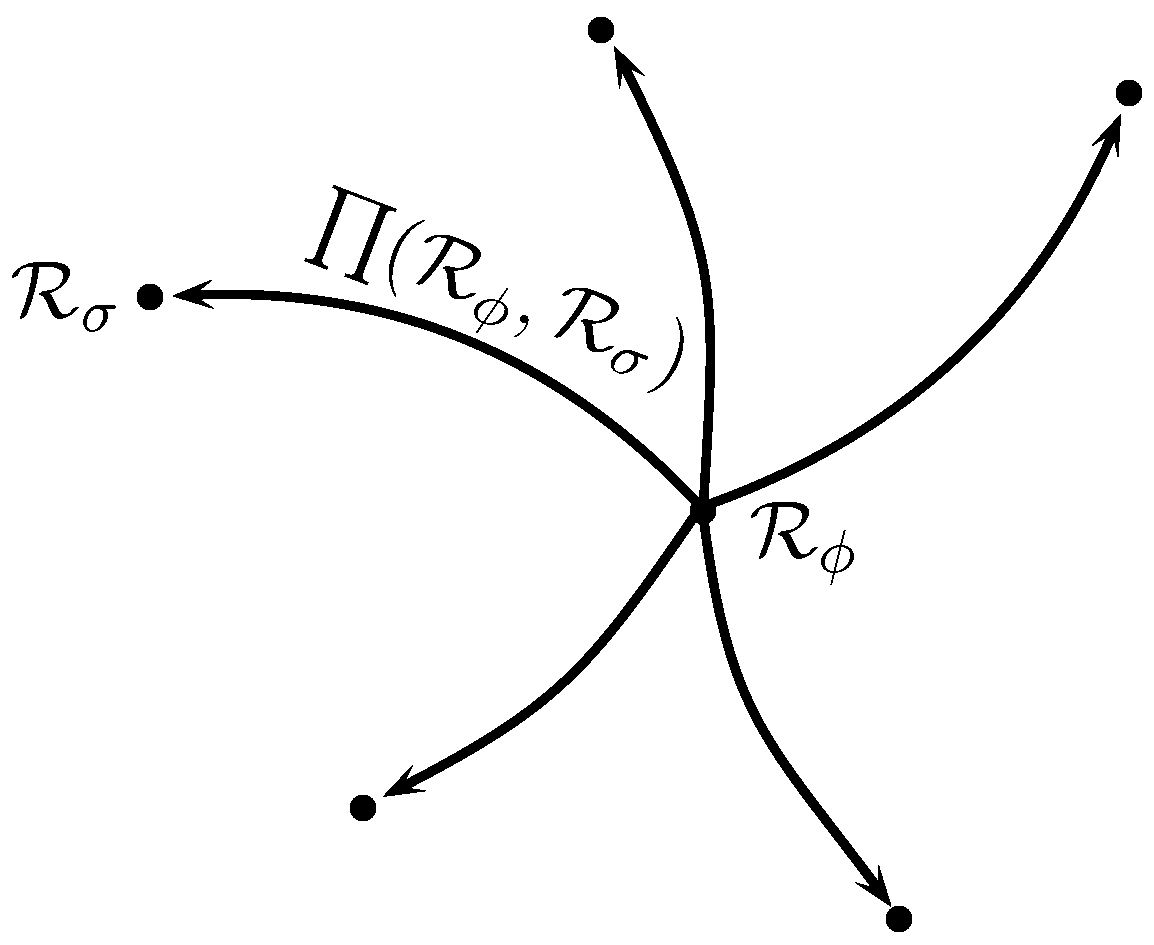
- The partial ranking of alternatives (or PROMETHEE I).The outgoing or leaving flow of an alternative is formulated as follows:that is, the outgoing flow of alternative is calculated as the average value of the arcs that are going outward form the node as shown in Figure 2. The outgoing flow is also known as the positive outranking flow and measures the dominance behavior of an alternative over all other alternatives.On the other hand, the incoming or entering flow of an alternative is calculated as follows:that is, the incoming flow of alternative is the average value of the inward arcs of the node as shown in Figure 3. The incoming flow is also known as the negative outranking flow and shows that how much an alternative is dominated by all other alternatives.The alternative with larger outgoing flow and the smaller incoming flow is considered as the favorable or preferable alternative. The preferences of alternatives on the basis of these positive and negative outranking flows can be computed by using the following expressions, respectively.The intersection of these two preferences provides the PROMETHEE I partial ranking of alternatives as follows:In PROMETHEE I partial ranking, all alternatives are not comparable, so the complete ranking of alternatives is obtained by proceeding the one more step of PROMETHEE II as follows.
- (b)
- Complete ordering of alternatives (or PROMETHEE II).The net outranking flow of alternative is calculated as,which is the difference of positive and negative flows and provides the PROMETHEE II complete ranking of alternatives in the following manner,Thus, all the alternatives can be compared on the basis of net flow of alternatives. The alternative with greatest net outranking flow is considered as the optimal solution or the most preferable alternative.
The procedure of mF PROMETHEE method is summarized in a flow chart as shown in Figure 4.
A series of steps and the number of calculations are involved in this multi-criteria decision-making method, in which all steps remain same except the choice of preference function. The preference function is defined according to the nature of criteria or by the choice of experts or analysts. Moreover, the criteria weights that are used to determine the multi-criteria preference index can be calculated by applying some appropriate method of normalized weights or can be taken regarding to the preferences of decision makers.
4. Ranking the Sites of Hydroelectric Power Stations
The electricity is considered as one of the main necessities or requirements for the economic development of a nation. The shortage of electricity not only affects the households, but also the economy. Due to the high and increasing demand of electricity, every state or country needs to generate their own energy without relying on international sources. There are many ways to convert different types of energies into electrical energy, including windmills, solar power, hydroelectric power and by burning the fossil fuels such as coal, oil or natural gas etc. Hydroelectric power is a renewable source of energy as it produces electricity by using the energy of flowing water. Moreover, it doesn’t pollute the environment like other power plants that use the coal or natural gas as fuel, therefore it is also known as clean fuel source of energy. Assume that a company wants to plant his own power station to fulfill the requirements of electricity. The suitable location or site is one of the most important factors to planted a hydroelectric power station. After initial screening, a set of seven different sites, , were selected for further evaluation. A committee of two field experts was appointed as decision makers to rank these sites on the basis of six criteria (or factors) as follows:
- Infrastructure,
- Nature of land,
- Government incentives,
- Social infrastructure,
- Climate changes,
- Cost.
Each factor has been further categorized into three characteristics to make a 3F number as follows:
- The factor “Infrastructure” includes the availability of water, storage of water and transportation facilities.
- The factor “Nature of land” includes the security level, availability of labor and soil type.
- The factor “Government incentives” includes the licensing policies, tax incentives and energy subsidies.
- The factor “Social infrastructure” includes the public safety, health care facilities and educational institutes.
- The factor “Climate changes” includes the atmospheric pressure, wind velocity and air temperature.
- The factor “Cost” includes the construction cost, maintenance cost and transportation cost.
On the basis of above discussed structure, the ranking for the sites of hydroelectric power plants by using PROMETHEE method is described as follows.
4.1. Criteria Weights by AHP
Firstly, the weights of criteria are calculated by using the process of AHP technique. The pairwise comparison of criteria are constructed on the basis of Saaty (1–9) preference scale as given in Table 1, and the values are given in Table 3.
By using the condition of normality, which is given in Equation (8), the normalized matrix for criteria is constructed as follows,
Then the criteria weights are calculated by employing the Equation (9) and the weights are provided in the column weight vector W as follows,
Next, we need to check the consistency of calculated weights by determining the consistency ratio of the comparison matrix. The small consistencies are negligible and do not cause the serious difficulties. For the consistency check, first step is to construct a matrix given as,
Then the maximum Eigenvalue is computed by applying the Equation (10), that is,
The consistency index is , which is obtained by employing the Equation (11), and the consistency ratio is determined by using the random index, (for ). Since the consistency ratio is , which is less than , so the given comparison matrix shows the consistent behavior and the calculated wights are appropriate for decision making.
4.2. Ranking through mF PROMETHEE
In this subsection, a new version of an outranking method PROMETHEE, named as mF PROMETHEE, is applied to rank the sites with respect to six criteria. The types of criteria, which are specified by decision maker on the basis of generalized criteria preference functions, and their corresponding parameters are given in Table 4.
The evaluations for ranking the sites of hydroelectric power plants through mF PROMETHEE method by applying the AHP weights of criteria are as follows.
- Step 1.
- The decision values of alternatives with respect to multiple and conflicting criteria in the form of 3F numbers are provided by experts and as shown in Table 5 and Table 6, respectively. Then the aggregated decision preferences are obtained by applying the averaging operator, and the results are summarized in Table 7.
- Step 2.
- The score matrix is constructed by applying the score function of 3F numbers as follows:
- Step 3.
- The score matrix is then used to calculate the difference or deviation of an alternative with respect to other alternatives. The deviation for every pair of alternatives with respect to each criterion is computed by using the Equation (15), and the outcomes are shown in Table 8.
- Step 4.
- Further, the preference degree of every pair of alternatives with respect to each criterion is calculated by using the preference function. In this method, six different types of preference functions are used according to the nature or type of criteria as described in Table 4. The results for each type of preference functions for every pair of alternatives are shown in Table 9.
- Step 5.
- Step 6.
- The whole procedure is concluded in this step and the results for partial and net outranking flows are determined.
- (a)
- Partial ranking of alternatives (or PROMETHEE I)The outgoing and incoming flows of alternatives are computed by employing Equations (20) and (21), respectively, and the results are summarized in Table 11.Then the partial raking of alternatives is determined by considering the intersection of preorders and , as follows:and the partial relations of PROMETHEE I are shown in Figure 5.
- (b)
- Complete ranking of alternatives (or PROMETHEE II)The net outranking flows of alternatives are computed by employing the Equation (25), and the net values are given in Table 12.It can be easily seen that the alternative is selected as the most suitable site for planting a hydroelectric power station, and the ordering of alternatives is given as,
5. Comparative Analysis
5.1. With Usual Criterion Preference Function
The choice of different types of preference functions for different criteria is one of the main advantages of PROMETHEE method. In Section 4.2, six different types of generalized criteria preference functions are considered for all six criteria to chose the most suitable site or location. In this subsection, only the usual criterion preference function is considered for all criteria for the location problem of hydroelectric power plant in order to provide the comparison of net results and to check the authenticity of proposed mF PROMETHEE method. The same weights are used which were calculated by AHP method in Section 4.1, and the steps for the construction of score matrix were same as enumerated in Section 4.2, so we proceed onward to Step 4.
- Step 4.
- The preference degree of each pair of alternative is computed by considering the usual criterion preference function for all criteria. In the case of criterion to be maximized, a strict preference is achieved only if there is a positive deviation between any pair of alternatives with respect to that criterion. On the other hand, the negative deviation between any pair of alternatives provides a strict preference in the case of criteria to be minimized. The results for the usual criterion preference functions are summarized in Table 13.
- Step 5.
- Step 6.
- The partial and net outranking flows of alternatives are calculated as follows.
- (a)
- The outgoing and incoming flows of alternatives are computed by using Equations (20) and (21), respectively, and the results of these flows are summarized in Table 15.The intersection of preorders and provides the partial ordering of alternatives or the partial results of PROMETHEE I, which is given as follows,and the partial relations of PROMETHEE I are shown in Figure 6.
- (b)
- The net outranking flows of alternatives are determined by applying Equation (25), and the results are given in Table 16.It is obvious from the net flows of alternatives that the alternative is chosen as the best suitable site and the ranking of different sites is given as follow,
The final ranking for the sites of hydroelectric power stations are given in Table 17, which is obtained by applying different types of preference functions under mF PROMETHEE method. It can easily be seen that is chosen as the most suitable alternative from both types of functions. Although the ranking of the sites obtained from different preference functions are not same, but the optimal solution remains same which shows that the preference function does not have an impact on the first-ranked alternative.
5.2. With m-Polar Fuzzy ELECTRE I
In this subsection, the location problem of hydroelectric power plant is solved by using the existing MCDM approach mF ELECTRE I method, which was presented by Akram et al. [18], and made a comparison of net results. Consider the aggregated decision matrix as given in Table 7 and the weights of criteria which were calculated by AHP method. Then the weighted aggregated decision matrix is constructed as given in Table 18, and follow the next steps of mF ELECTRE I method to determine an outranking relation of alternatives in account to make a comparison of these multi-attribute decision making methods.
The evaluation of mF concordance sets , mF discordance sets , mF concordance indices , mF discordance indices , concordance dominance , discordance dominance , aggregated dominance and outranking relations for this location problem is briefly summarized in Table 19. The graph sketch by outranking relations is given in Figure 7 and the set of most favorable alternatives is . It can be easily seen that the alternative is chosen as the best possible location for all these MCDM methods under mF environment. So, mF PROMETHEE method can successfully be applied to solve the MCDM problems with mF information. Different versions of this method not only provide the kernel solution, but also produce the ranking of alternatives in a descending order.
6. Conclusions
Many real-world problems have multi-polarity in decision data that can be properly describe with the help of multiple attributes. As a number of theoretical models have been developed to encompass the wider range of decision data, the combination of these models with MCDA techniques can provide the more accurate and authentic results of complex decision problems.
In this research article we have proposed a MCDA technique that makes an efficient use of mF information, and we named it as the AHP-assisted mF PROMETHEE method. It consists of two parts, namely, the calculation of the weights of the criteria and the ranking of the set of feasible alternatives. The normalized weights of the attributes are determined by the AHP technique. Then a novel variation of the PROMETHEE approach produces the ranking of alternatives in the context of mF numbers.
As an application, the combination of six types of generalized criteria preference functions delivered partial and complete rankings of hydroelectric power plants. Moreover, the comparative analysis of net obtained results was provided by assigning the usual criterion preference function for all criteria. Furthermore, the reliability of this method has been analyzed by applying an existing MCDM approach, such as mF ELECTRE I method, to the same location problem. It can be easily observe that the different versions of proposed mF PROMETHEE technique not only provide the solution set but also ranks all the alternatives in a descending order as compared to mF ELECTRE I method.
This research analysis is limited in a way that the net outranking flow of alternatives are calculated by using the simple subtraction arithmetic function. This limitation can be addressed by using the different arithmetic functions or any distance formula in future work. In future research, we aim at extending our work to the cases of (1) the complex fuzzy PROMETHEE technique; (2) the bipolar neutrosophic PROMETHEE method; and (3) the bipolar fuzzy soft PROMETHEE method.
Author Contributions
Conceptualization: S. Methodology and Supervision: M.A. Formal analysis: M.A., S., J.C.R.A. Roles/Writing—original draft preparation: M.A., S. Writing—review & editing: J.C.R.A. All authors have read and agree to the published version of the manuscript.
Funding
This research received no external funding.
Conflicts of Interest
The authors declare no conflict of interest.
References
- Teixeira, C.; Lopes, I.; Figueiredo, M. Classification methodology for spare parts management combining maintenance and logistics perspectives. J. Manag. Anal. 2018, 5, 116–135. [Google Scholar] [CrossRef]
- Alcantud, J.C.R.; Cruz-Rambaud, S.; Muñoz Torrecillas, M.J. Valuation fuzzy soft sets: A flexible fuzzy soft set based decision making procedure for the valuation of assets. Symmetry 2017, 9, 253. [Google Scholar] [CrossRef] [Green Version]
- Alcantud, J.C.R.; Khameneh, A.Z.; Kilicman, A. Aggregation of infinite chains of intuitionistic fuzzy sets and their application to choices with temporal intuitionistic fuzzy information. Inf. Sci. 2020, 514, 106–117. [Google Scholar] [CrossRef]
- Xia, M.; Xu, Z.; Chen, N. Some hesitant fuzzy aggregation operators with their application in group decision making. Group Decis. Negot. 2013, 22, 259–279. [Google Scholar] [CrossRef]
- Zavadskas, E.K.; Antucheviciene, J.; Vilutiene, T.; Adeli, H. Sustainable decision-making in civil engineering, construction and building technology. Sustainability 2018, 10, 14. [Google Scholar] [CrossRef] [Green Version]
- Hwang, C.L.; Yoon, K. Multiple Attribute Decision Making Methods and Applications; Springer: Berlin, Germany, 1981. [Google Scholar]
- Opricovic, S.; Tzeng, G.H. Compromise solution by MCDM methods: A comparative analysis of VIKOR and TOPSIS. Eur. J. Oper. Res. 2004, 156, 445–455. [Google Scholar] [CrossRef]
- Benayoun, R.; Roy, B.; Sussman, B. ELECTRE: Une Méthode pour Guider le Choix en Présence de Points de Vue Multiples; Direction Scientifique SEMA: Paris, France, 1966. [Google Scholar]
- Brans, J.P.; Vincke, P. A preference ranking organization method (The PROMETHEE method for multiple criteria decision making). Manag. Sci. 1985, 31, 647–656. [Google Scholar] [CrossRef] [Green Version]
- Zadeh, L.A. Fuzzy sets. Inf. Control 1965, 8, 338–353. [Google Scholar] [CrossRef] [Green Version]
- Zhang, W.R. Bipolar fuzzy sets and relations: A computational framework for cognitive modeling and multiagent decision analysis. In Proceedings of the IEEE Conference Fuzzy Information Processing Society Biannual Conference, San Antonio, TX, USA, 18–21 December 1994; pp. 305–309. [Google Scholar]
- Akram, M.; Arshad, M. A novel trapezoidal bipolar fuzzy TOPSIS method for group decision-making. Group Decis. Negot. 2019, 28, 565–584. [Google Scholar] [CrossRef]
- Akram, M.; Shumaiza; Arshad, M. Bipolar fuzzy TOPSIS and bipolar fuzzy ELECTRE-I methods to diagnosis. Comput. Appl. Math. 2020, 39, 1–23. [Google Scholar] [CrossRef]
- Shumaiza; Akram, M.; Al-Kenani, A.N.; Alcantud, J.C.R. Group decision-making based on the VIKOR method with trapezoidal bipolar fuzzy information. Symmetry 2019, 11, 1–21. [Google Scholar]
- Shumaiza; Akram, M.; Al-Kenani, A.N. Multiple-Attribute Decision Making ELECTRE II Method under bipolar fuzzy model. Algorithms 2019, 12, 226. [Google Scholar] [CrossRef] [Green Version]
- Akram, M.; Shumaiza; Al-Kenani, A.N. Multi-criteria group decision-making for selection of green suppliers under bipolar fuzzy PROMETHEE process. Symmetry 2020, 12, 77. [Google Scholar] [CrossRef] [Green Version]
- Chen, J.; Li, S.; Ma, S.; Wang, X. m-polar fuzzy sets: An extension of bipolar fuzzy sets. Sci. World J. 2014, 2014, 416530. [Google Scholar] [CrossRef] [PubMed] [Green Version]
- Akram, M.; Waseem, N.; Liu, P. Novel approach in decision making with m-polar fuzzy ELECTRE-I. Int. J. Fuzzy Syst. 2019, 21, 1117–1129. [Google Scholar] [CrossRef]
- Adeel, A.; Akram, M.; Koam, A.N. Group decision-making based on m-polar fuzzy linguistic TOPSIS method. Symmetry 2019, 11, 735. [Google Scholar] [CrossRef] [Green Version]
- Saaty, T.L. Axiomatic foundation of the analytic hierarchy process. Manag. Sci. 1986, 32, 841–855. [Google Scholar] [CrossRef]
- Lee, J.W.; Kim, S.H. Using analytic network process and goal programming for interdependent information system project selection. Comput. Oper. Res. 2000, 27, 367–382. [Google Scholar] [CrossRef]
- Charnes, A.; Cooper, W.; Lewin, A.Y.; Seiford, L.M. Data envelopment analysis theory, methodology and applications. J. Oper. Res. Soc. 1997, 48, 332–333. [Google Scholar] [CrossRef]
- Julong, D. Introduction to grey system theory. J. Grey Syst. 1989, 1, 1–24. [Google Scholar]
- Bellman, R.E.; Zadeh, L.A. Decision-making in a fuzzy environment. Manag. Sci. 1970, 4, 141–164. [Google Scholar] [CrossRef]
- San Cristóbal, J.R. Multi-criteria decision-making in the selection of a renewable energy project in Spain: The VIKOR method. Renew. Energy 2011, 36, 498–502. [Google Scholar] [CrossRef]
- Moreno-Jimenez, J.M.; Aguaron, J.; Escobar, M.T. The core of consistency in AHP-group decision making. Group Decis. Negot. 2008, 17, 249–265. [Google Scholar] [CrossRef]
- Karim, R.; Karmaker, C.L. Machine selection by AHP and TOPSIS methods. Am. J. Ind. Eng. 2016, 4, 7–13. [Google Scholar]
- Shahroodi, K.; Amin, K.; Shabnam, A.; Elnaz, S.; Najibzadeh, M. Application of analytical hierarchy process (AHP) technique to evaluate and selecting suppliers in an effective supply chain. Kuwait Chapter Arab. J. Bus. Manag. Rev. 2012, 33, 1–14. [Google Scholar]
- Chang, D.Y. Applications of the extent analysis method on fuzzy AHP. Eur. J. Oper. Res. 1996, 95, 649–655. [Google Scholar] [CrossRef]
- Junior, F.R.L.; Osiro, L.; Carpinetti, L.C.R. A comparison between fuzzy AHP and fuzzy TOPSIS methods to supplier selection. Appl. Soft Comput. 2014, 21, 194–209. [Google Scholar] [CrossRef]
- Liu, P.; Chen, S.M.; Wang, Y. Multiattribute group decision making based on intuitionistic fuzzy partitioned Maclaurin symmetric mean operators. Inf. Sci. 2020, 512, 830–854. [Google Scholar] [CrossRef]
- Liu, P.; Wang, Y. Multiple attribute decision making based on q-rung orthopair fuzzy generalized Maclaurin symmetric mean operators. Inf. Sci. 2020, 518, 181–210. [Google Scholar] [CrossRef]
- Zhan, J.; Sun, B.; Zhang, X. PF-TOPSIS method based on CPFRS models: An application to unconventional emergency events. Comput. Ind. Eng. 2020, 139, 106192. [Google Scholar] [CrossRef]
- Zhang, K.; Zhan, J.; Wu, W.; Alcantud, J.C.R. Fuzzy β-covering based (I, T)-fuzzy rough set models and applications to multi-attribute decision-making. Comput. Ind. Eng. 2019, 128, 605–621. [Google Scholar] [CrossRef]
- Brans, J.P.; Vincke, P.; Mareschal, B. How to select and how to rank projects: The PROMETHEE method. Eur. J. Oper. Res. 1986, 24, 228–238. [Google Scholar] [CrossRef]
- Abdullah, L.; Chan, W.; Afshari, A. Application of PROMETHEE method for green supplier selection: A comparative result based on preference functions. J. Ind. Eng. Int. 2019, 15, 271–285. [Google Scholar] [CrossRef] [Green Version]
- Behzadian, M.; Kazemzadeh, R.B.; Albadvi, A.; Aghdasi, M. PROMETHEE: A comprehensive literature review on methodologies and applications. Eur. J. Oper. Res. 2010, 200, 198–215. [Google Scholar] [CrossRef]
- Govindan, K.; Kadzinski, M.; Sivakumar, R. Application of a novel PROMETHEE-based method for construction of a group compromise ranking to prioritization of green suppliers in food supply chain. Omega 2017, 71, 129–145. [Google Scholar] [CrossRef]
- Goumas, M.; Lygerou, V. An extension of the PROMETHEE method for decision making in fuzzy environment: Ranking of alternative energy exploitation projects. Eur. J. Oper. Res. 2000, 123, 606–613. [Google Scholar] [CrossRef]
- Krishankumar, R.; Ravichandran, K.S.; Saeid, A.B. A new extension to PROMETHEE under intuitionistic fuzzy environment for solving supplier selection problem with linguistic preferences. Appl. Soft Comput. 2017, 60, 564–576. [Google Scholar]
- Ziemba, P. NEAT F-PROMETHEE—A new fuzzy multiple criteria decision making method based on the adjustment of mapping trapezoidal fuzzy numbers. Expert Syst. Appl. 2018, 110, 363–380. [Google Scholar] [CrossRef]
- Alcantud, J.C.R.; Biondo, A.E.; Giarlotta, A. Fuzzy politics I: The genesis of parties. Fuzzy Sets Syst. 2018, 349, 71–98. [Google Scholar] [CrossRef]
Figure 1.
Preference function.

Figure 2.
Outgoing flow of .

Figure 3.
Incoming flow of .

Figure 4.
Flow chart of mF PROMETHEE method.

Figure 5.
Partial relations of PROMETHEE I.

Figure 6.
Partial relations of PROMETHEE I.

Figure 7.
Graph representing the outranking relation of alternatives.


Table 1.
Saaty (1–9) Preference Scale.
| Scale | Definition | Explanation |
|---|---|---|
| 1 | Equally Important | Both criteria participate equally to the goal |
| 3 | Weakly Important | Experience weakly favor of one criterion over another |
| 5 | Strongly Important | Experience strongly favor of one criterion over another |
| 7 | Very Strongly Important | Strong dominance of one criterion over another |
| 9 | Extremely Important | The preference of a criterion is of the highest possible value |
| Intermediate values between adjacent scales | When compromise is required |
Table 2.
Random index for different values of n.
| n | 2 | 3 | 4 | 5 | 6 | 7 | 8 | 9 | 10 |
| RI | 0 | 0.58 | 0.90 | 1.12 | 1.24 | 1.32 | 1.41 | 1.45 | 1.49 |
Table 3.
The pairwise comparison of criteria.
| 1 | 5 | 9 | 3 | 5 | 7 | |
| 1 | 5 | 5 | ||||
| 1 | ||||||
| 3 | 5 | 1 | 1 | 3 | ||
| 3 | 7 | 1 | 1 | 5 | ||
| 3 | 1 |
Table 4.
Types of criteria and corresponding parameters.
| Criteria | Max or Min | Type of Criterion | Parameters |
|---|---|---|---|
| Max | V | , | |
| Max | III | ||
| Min | VI | ||
| Max | II | ||
| Min | IV | , | |
| Min | I | - |
Table 5.
Decision values of alternatives by decision maker .
| Infrastructure | Nature of Land | Government Incentives | |
| Social Infrastructure | Climate Changes | Cost | |
Table 6.
Decision values of alternatives by decision maker .
| Infrastructure | Nature of Land | Government Incentives | |
| Social Infrastructure | Climate Changes | Cost | |
Table 7.
Aggregated decision values of alternatives.
| Infrastructure | Nature of Land | Government Incentives | |
| Social Infrastructure | Climate Changes | Cost | |
Table 8.
Deviation of alternatives with respect to criteria.
| −0.105 | −0.191 | 0.065 | 0.017 | −0.131 | −0.15 | |
| −0.06 | −0.01 | −0.016 | −0.113 | 0.079 | −0.065 | |
| −0.147 | 0.014 | −0.041 | −0.045 | 0.084 | −0.011 | |
| −0.097 | −0.056 | −0.025 | −0.041 | 0.064 | 0.025 | |
| −0.194 | −0.045 | −0.021 | −0.063 | 0.004 | 0.039 | |
| −0.085 | −0.02 | −0.146 | −0.136 | 0.062 | 0.45 | |
| 0.105 | 0.191 | −0.065 | −0.017 | 0.131 | 0.15 | |
| 0.045 | 0.181 | −0.081 | −0.31 | 0.21 | 0.085 | |
| −0.042 | 0.205 | −0.106 | −0.062 | 0.215 | 0.319 | |
| 0.008 | 0.135 | −0.09 | −0.058 | 0.195 | 0.175 | |
| −0.089 | 0.146 | −0.086 | −0.08 | 0.135 | 0.189 | |
| 0.02 | 0.171 | −0.211 | −0.153 | 0.193 | 0.195 | |
| 0.06 | 0.01 | 0.016 | 0.113 | −0.079 | 0.065 | |
| −0.045 | −0.181 | 0.081 | 0.13 | −0.21 | −0.085 | |
| −0.087 | 0.024 | −0.025 | 0.068 | 0.005 | 0.054 | |
| −0.037 | −0.046 | −0.009 | 0.072 | −0.015 | 0.09 | |
| −0.134 | −0.035 | −0.005 | 0.05 | −0.075 | 0.104 | |
| −0.025 | −0.01 | −0.13 | −0.023 | −0.017 | 0.11 | |
| 0.147 | −0.014 | 0.041 | 0.045 | −0.084 | 0.011 | |
| 0.042 | −0.205 | 0.106 | 0.062 | −0.215 | −0.139 | |
| 0.087 | −0.024 | 0.025 | −0.068 | −0.005 | −0.054 | |
| 0.05 | −0.07 | 0.016 | 0.004 | −0.02 | 0.036 | |
| −0.047 | −0.059 | 0.02 | −0.018 | −0.08 | 0.05 | |
| 0.062 | −0.034 | −0.105 | −0.091 | −0.022 | 0.056 | |
| 0.097 | 0.056 | 0.025 | 0.041 | −0.064 | −0.025 | |
| −0.008 | −0.135 | 0.09 | 0.058 | −0.195 | −0.175 | |
| 0.037 | 0.046 | 0.009 | −0.072 | 0.015 | −0.09 | |
| −0.05 | 0.07 | −0.016 | −0.004 | 0.02 | −0.036 | |
| −0.097 | 0.011 | 0.004 | −0.022 | −0.06 | 0.014 | |
| 0.012 | 0.036 | −0.121 | −0.095 | −0.002 | 0.02 | |
| 0.194 | 0.045 | 0.021 | 0.063 | −0.004 | −0.039 | |
| 0.089 | −0.146 | 0.086 | 0.08 | −0.135 | −0.189 | |
| 0.134 | 0.035 | 0.005 | −0.05 | 0.075 | −0.104 | |
| 0.047 | 0.059 | −0.02 | 0.018 | 0.08 | −0.05 | |
| 0.097 | −0.011 | −0.004 | 0.022 | 0.06 | −0.014 | |
| 0.109 | 0.025 | −0.125 | −0.073 | 0.058 | 0.006 | |
| 0.085 | 0.02 | 0.146 | 0.136 | −0.062 | −0.045 | |
| −0.02 | −0.171 | 0.211 | 0.153 | −0.193 | −0.195 | |
| 0.025 | 0.01 | 0.13 | 0.023 | 0.017 | −0.11 | |
| −0.062 | 0.034 | 0.105 | 0.091 | 0.022 | −0.056 | |
| −0.012 | −0.036 | 0.121 | 0.095 | 0.002 | −0.02 | |
| −0.109 | −0.025 | 0.125 | 0.073 | −0.058 | −0.006 |
Table 9.
Generalized criteria preference function.
| 0.00 | 0.00 | 0.00 | 1.00 | 1.00 | 1.00 | |
| 0.00 | 0.00 | 0.03 | 0.00 | 0.00 | 1.00 | |
| 0.00 | 0.14 | 0.15 | 0.00 | 0.00 | 1.00 | |
| 0.00 | 0.00 | 0.06 | 0.00 | 0.00 | 0.00 | |
| 0.00 | 0.00 | 0.04 | 0.00 | 0.00 | 0.00 | |
| 0.00 | 0.00 | 0.88 | 0.00 | 0.00 | 0.00 | |
| 1.00 | 1.00 | 0.34 | 0.00 | 0.00 | 0.00 | |
| 0.25 | 1.00 | 0.48 | 0.00 | 0.00 | 0.00 | |
| 0.00 | 1.00 | 0.67 | 0.00 | 0.00 | 0.00 | |
| 0.00 | 1.00 | 0.56 | 0.00 | 0.00 | 0.00 | |
| 0.00 | 1.00 | 0.52 | 0.00 | 0.00 | 0.00 | |
| 0.00 | 1.00 | 0.99 | 0.00 | 0.00 | 0.00 | |
| 0.40 | 0.10 | 0.00 | 1.00 | 0.50 | 0.00 | |
| 0.00 | 0.00 | 0.00 | 1.00 | 1.00 | 1.00 | |
| 0.00 | 0.24 | 0.06 | 1.00 | 0.00 | 0.00 | |
| 0.00 | 0.00 | 0.01 | 1.00 | 0.00 | 0.00 | |
| 0.00 | 0.00 | 0.002 | 1.00 | 0.50 | 0.00 | |
| 0.00 | 0.00 | 0.82 | 0.00 | 0.00 | 0.00 | |
| 1.00 | 0.00 | 0.00 | 1.00 | 0.50 | 0.00 | |
| 0.22 | 0.00 | 0.00 | 1.00 | 1.00 | 1.00 | |
| 0.67 | 0.00 | 0.00 | 0.00 | 0.00 | 1.00 | |
| 0.30 | 0.00 | 0.00 | 0.00 | 0.00 | 0.00 | |
| 0.00 | 0.00 | 0.00 | 0.00 | 0.50 | 0.00 | |
| 0.42 | 0.00 | 0.67 | 0.00 | 0.00 | 0.00 | |
| 0.77 | 0.56 | 0.00 | 1.00 | 0.50 | 1.00 | |
| 0.00 | 0.00 | 0.00 | 1.00 | 1.00 | 1.00 | |
| 0.17 | 0.46 | 0.00 | 0.00 | 0.00 | 1.00 | |
| 0.00 | 0.70 | 0.03 | 0.00 | 0.00 | 1.00 | |
| 0.00 | 0.11 | 0.00 | 0.00 | 0.50 | 0.00 | |
| 0.00 | 0.36 | 0.77 | 0.00 | 0.00 | 0.00 | |
| 1.00 | 0.45 | 0.00 | 1.00 | 0.00 | 1.00 | |
| 0.69 | 0.00 | 0.00 | 1.00 | 1.00 | 1.00 | |
| 1.00 | 0.35 | 0.00 | 0.00 | 0.00 | 1.00 | |
| 0.27 | 0.59 | 0.04 | 1.00 | 0.00 | 1.00 | |
| 0.77 | 0.00 | 0.002 | 1.00 | 0.00 | 1.00 | |
| 1.00 | 0.25 | 0.79 | 0.00 | 0.00 | 0.00 | |
| 0.65 | 0.20 | 0.00 | 1.00 | 0.50 | 1.00 | |
| 0.00 | 0.00 | 0.00 | 1.00 | 1.00 | 1.00 | |
| 0.05 | 0.10 | 0.00 | 1.00 | 0.00 | 1.00 | |
| 0.00 | 0.34 | 0.00 | 1.00 | 0.00 | 1.00 | |
| 0.00 | 0.00 | 0.00 | 1.00 | 0.00 | 1.00 | |
| 0.00 | 0.00 | 0.00 | 1.00 | 0.50 | 1.00 |
Table 10.
Multi-criteria preference index.
| - | |||||||
| - | |||||||
| - | |||||||
| - | |||||||
| - | |||||||
| - | |||||||
| - |
Table 11.
Positive and negative outranking flows.
| Alternatives | ||
|---|---|---|
Table 12.
Net flow of alternatives.
| Alternatives | |
|---|---|
| 0.130 | |
| 0.063 | |
| 0.433 | |
| 0.192 |
Table 13.
Usual criterion preference function.
| 0 | 0 | 0 | 1 | 1 | 1 | |
| 0 | 0 | 1 | 0 | 0 | 1 | |
| 0 | 1 | 1 | 0 | 0 | 1 | |
| 0 | 0 | 1 | 0 | 0 | 0 | |
| 0 | 0 | 1 | 0 | 0 | 0 | |
| 0 | 0 | 1 | 0 | 0 | 0 | |
| 1 | 1 | 1 | 0 | 0 | 0 | |
| 1 | 1 | 1 | 0 | 0 | 0 | |
| 0 | 1 | 1 | 0 | 0 | 0 | |
| 1 | 1 | 1 | 0 | 0 | 0 | |
| 0 | 1 | 1 | 0 | 0 | 0 | |
| 1 | 1 | 1 | 0 | 0 | 0 | |
| 1 | 1 | 0 | 1 | 1 | 0 | |
| 0 | 0 | 0 | 1 | 1 | 1 | |
| 0 | 1 | 1 | 1 | 0 | 0 | |
| 0 | 0 | 1 | 1 | 1 | 0 | |
| 0 | 0 | 1 | 1 | 1 | 0 | |
| 0 | 0 | 1 | 0 | 1 | 0 | |
| 1 | 0 | 0 | 1 | 1 | 0 | |
| 1 | 0 | 0 | 1 | 1 | 1 | |
| 1 | 0 | 0 | 0 | 1 | 1 | |
| 1 | 0 | 0 | 1 | 1 | 0 | |
| 0 | 0 | 0 | 0 | 1 | 0 | |
| 1 | 0 | 1 | 0 | 1 | 0 | |
| 1 | 1 | 0 | 1 | 1 | 1 | |
| 0 | 0 | 0 | 1 | 1 | 1 | |
| 1 | 1 | 0 | 0 | 0 | 1 | |
| 0 | 1 | 1 | 0 | 0 | 1 | |
| 0 | 1 | 0 | 0 | 1 | 0 | |
| 1 | 1 | 1 | 0 | 1 | 0 | |
| 1 | 1 | 0 | 1 | 1 | 1 | |
| 1 | 0 | 0 | 1 | 1 | 1 | |
| 1 | 1 | 0 | 0 | 0 | 1 | |
| 1 | 1 | 1 | 1 | 0 | 1 | |
| 1 | 0 | 1 | 1 | 0 | 1 | |
| 1 | 1 | 1 | 0 | 0 | 0 | |
| 1 | 1 | 0 | 1 | 1 | 1 | |
| 0 | 0 | 0 | 1 | 1 | 1 | |
| 1 | 1 | 0 | 1 | 0 | 1 | |
| 0 | 1 | 0 | 1 | 0 | 1 | |
| 0 | 0 | 0 | 1 | 0 | 1 | |
| 0 | 0 | 0 | 1 | 1 | 1 |
Table 14.
Multi-criteria preference index.
| - | |||||||
| - | |||||||
| - | |||||||
| - | |||||||
| - | |||||||
| - | |||||||
| - |
Table 15.
Positive and negative outranking flows.
| Alternatives | ||
|---|---|---|
Table 16.
Net flow of alternatives.
| Alternatives | |
|---|---|
Table 17.
Final ranking of hydroelectric power plants.
| Alternatives | Combination of Six Preference Functions | Usual Criterion Preference Function |
|---|---|---|
| 7 | 7 | |
| 6 | 5 | |
| 5 | 6 | |
| 3 | 2 | |
| 4 | 3 | |
| 1 | 1 | |
| 2 | 4 |
Table 18.
Weighted aggregated decision matrix.
| Infrastructure | Nature of Land | Government Incentives | |
| Social Infrastructure | Climate Changes | Cost | |
Table 19.
mF ELECTRE I results for selection of hydroelectric power plant.
| Alternatives Compared | Outranking Relations | |||||||
|---|---|---|---|---|---|---|---|---|
| 1 | 0 | 0 | 0 | Incomparable | ||||
| 1 | 0 | 0 | 0 | Incomparable | ||||
| 1 | 0 | 0 | 0 | Incomparable | ||||
| 1 | 0 | 0 | 0 | Incomparable | ||||
| 1 | 0 | 0 | 0 | Incomparable | ||||
| 1 | 0 | 0 | 0 | Incomparable | ||||
| 1 | 1 | 1 | ||||||
| 1 | 1 | 1 | ||||||
| 0 | 1 | 0 | Incomparable | |||||
| {1,2,5,6} | 1 | 1 | 1 | |||||
| 0 | 1 | 0 | Incomparable | |||||
| {1,2,5,6} | 1 | 1 | 1 | |||||
| ) | 1 | 1 | 1 | |||||
| 1 | 0 | 0 | 0 | Incomparable | ||||
| 1 | 1 | 0 | 0 | Incomparable | ||||
| 1 | 0 | 0 | 0 | Incomparable | ||||
| 1 | 0 | 0 | 0 | Incomparable | ||||
| 1 | 0 | 0 | 0 | Incomparable | ||||
| 1 | 1 | 1 | ||||||
| 1 | 1 | 0 | 0 | Incomparable | ||||
| 0 | 1 | 0 | Incomparable | |||||
| 1 | 1 | 1 | ||||||
| 1 | 0 | 0 | 0 | Incomparable | ||||
| 1 | 1 | 1 | ||||||
| 1 | 1 | 1 | ||||||
| 1 | 0 | 0 | 0 | Incomparable | ||||
| 1 | 0 | 0 | Incomparable | |||||
| 1 | 0 | 0 | 0 | Incomparable | ||||
| 1 | 0 | 0 | 0 | Incomparable | ||||
| 1 | 1 | 0 | 0 | Incomparable | ||||
| 1 | 1 | 1 | ||||||
| 1 | 1 | 0 | 0 | Incomparable | ||||
| 1 | 1 | 1 | ||||||
| 1 | 1 | 1 | ||||||
| 1 | 1 | 1 | ||||||
| 1 | 1 | 1 | ||||||
| 1 | 1 | 1 | ||||||
| 1 | 0 | 0 | 0 | Incomparable | ||||
| 1 | 1 | 1 | ||||||
| 1 | 0 | 0 | 0 | Incomparable | ||||
| 0 | 1 | 0 | Incomparable | |||||
| 1 | 0 | 0 | 0 | Incomparable |
© 2020 by the authors. Licensee MDPI, Basel, Switzerland. This article is an open access article distributed under the terms and conditions of the Creative Commons Attribution (CC BY) license (http://creativecommons.org/licenses/by/4.0/).
Share and Cite
MDPI and ACS Style
Akram, M.; Shumaiza; Alcantud, J.C.R. An m-Polar Fuzzy PROMETHEE Approach for AHP-Assisted Group Decision-Making. Math. Comput. Appl. 2020, 25, 26. https://0-doi-org.brum.beds.ac.uk/10.3390/mca25020026
AMA Style
Akram M, Shumaiza, Alcantud JCR. An m-Polar Fuzzy PROMETHEE Approach for AHP-Assisted Group Decision-Making. Mathematical and Computational Applications. 2020; 25(2):26. https://0-doi-org.brum.beds.ac.uk/10.3390/mca25020026
Chicago/Turabian StyleAkram, Muhammad, Shumaiza, and José Carlos R. Alcantud. 2020. "An m-Polar Fuzzy PROMETHEE Approach for AHP-Assisted Group Decision-Making" Mathematical and Computational Applications 25, no. 2: 26. https://0-doi-org.brum.beds.ac.uk/10.3390/mca25020026