Porous Functionally Graded Plates: An Assessment of the Influence of Shear Correction Factor on Static Behavior

Abstract

The known multifunctional characteristic of porous graded materials makes them very attractive in a number of diversified application fields, which simultaneously poses the need to deepen research efforts in this broad field. The study of functionally graded porous materials is a research topic of interest, particularly concerning the modeling of porosity distributions and the corresponding estimations of their material properties—in both real situations and from a material modeling perspective. This work aims to assess the influence of different porosity distribution approaches on the shear correction factor, used in the context of the first-order shear deformation theory, which in turn may introduce significant effects in a structure’s behavior. To this purpose, we evaluated porous functionally graded plates with varying composition through their thickness. The bending behavior of these plates was studied using the finite element method with two quadrilateral plate element models. Verification studies were performed to assess the representativeness of the developed and implemented models, namely, considering an alternative higher-order model also employed for this specific purpose. Comparative analyses were developed to assess how porosity distributions influence the shear correction factor, and ultimately the static behavior, of the plates.

1. Introduction

Material science has undergone great evolution in recent years, representing an extremely important field for the development of many technological areas for several reasons, such as those related to a sustainable economic and environmental nature. The introduction of the functional gradient concept in the context of composite particulate materials has contributed to the design of advanced materials able to meet specific objectives, through spatial variation in composition and/or microstructure [1,2].

Functional gradient materials (FGMs) were developed in Japan in the late 1980s for thermal insulation coatings [2]. With more than three decades of history, and being a part of a wide variety of composite materials, materials with functional gradients continue to be the object of attention. This is due to their tailorability, arising from a gradual and continuous microstructure evolution and, consequently, of locally varying material properties in one or more spatial directions. Therefore, FGMs can be appropriately idealized to meet certain specifications [3,4].

Composite materials can generally be described as systems composed of a matrix and a reinforcement, the material properties of which surpass those presented by each constituent individually [5]. The gradual and continuous evolution of their material properties provide FGMs with better mechanical behavior than traditional composite materials [6]. Among other characteristics possessed by some FGMs, such as low thermal conductivity and low residual stresses, these materials also make it possible to minimize the stress discontinuities of conventional laminated composites [5,7,8]. FGMs’ high resistance to temperature and the absence of interface problems gives them great importance in several engineering applications, which is why these composite materials have been extensively studied and used in the past two decades in a wide range of science fields requiring improved mechanical and thermal performances [5,6,7]. This broad range of applications justifies the need to study and predict the responses of FGMs’ components [9]. In the past year, Li et al. developed several studies involving, among other topics, a stability and buckling analysis of functionally graded structures such as cylinders and arches [10,11,12,13,14].

Considering the continuous mixture concept behind their composition, FGMs can be constituted of two or more material phases. Hence, the resulting local material properties depend on this mixture evolution, allowing for a design according to the desired functions and specifications [15]. From the literature, the most common FGMs are constituted of two material phases, often one ceramic and one metal [6,11].

The manufacturing process of sintering, which is common in the production of FGMs, is responsible for the formation of micro voids or porosities within the materials, making important the introduction of porosity effects at the structures’ design stage [9]. The literature contains various studies which include dynamic and static analyses of functionally graded porous plates and beams [16,17,18,19,20,21]. In addition, there are several studies considering ring and arch structures, especially those developed by Li et al. in the past year [13,22,23,24,25,26,27].

Functionally graded porous materials (FGPs) combine both porosity and functional gradient characteristics, where the porosity may have a graded evolution across the volume, providing desirable properties for some applications (as in biomedical implants), and undesirable in others where voids may cause serious problems (as in the aeronautical sector). The change in porosity in one or more directions can be caused by local density effects or pore size alteration. Functionally graded porous materials possess a cell-based structure, which can be classified as open or closed (i.e., containing interconnected or isolated pores, respectively) [15].

Porous gradient materials also present a multifunctional character, where, among other aspects, one may highlight a high performance-to-weight ratio and resistance to shock; nevertheless, it is important to note that pores imply a local loss of stiffness. The latest advances in manufacturing processes allow the consideration of the development of porous materials with a functional gradient, using methods such as additive 3D printing. Thus, it becomes possible to design porous structures with designed variable stiffness, which can be customized for specific engineering applications, optimizing performance and minimizing weight [28]. Due to the relevant role that such materials have in a range of applications, it is important to have a wider perspective of the contexts where one can find them.

Mechanical or more generically structural components made of porous materials, bioinspired materials, can be designed for sensitive and very precise operating conditions—for example, robotic, prosthetic, and aeronautical components, among others [28]. Most of the materials used in engineering are dense; however, porous materials are also of great interest and applicability in fields such as in membranes [3]. Bioinspired materials thus have great potential for current technologies, as their unique characteristics allow them to meet various design requirements [28]. Natural or man-made, porous compacts or foams—the types of porous materials are many and diverse. Bones, wood, ceramics, and aluminum foams are just a few examples [29]. In the field of biomaterials, the inclusion of porosities allows diversification of their applicability, with ceramic and polymeric scaffolds being examples of this [3].

In the biomedical field, a bone implant must guarantee a functional gradient that mimics real bone stiffness variations. With functionally graded porous scaffolds it is possible to obtain the variations in mechanical and biological properties required for bone implants, as the presence of a porosity gradient is imperative for bone regeneration. Thus, functionally graded porous scaffolds for bone implants are designed to achieve the ideal balance between porosity and mechanical properties [30]. Since bone implants have various requirements, it is important to have ceramic porous materials with a wide and diversified range of pore sizes and morphologies in order to accomplish these requirements. Therefore, different porous hydroxyapatite structures have been developed to mimic natural bone’s bimodal structure [31]. Since implants with no porosity show weak tissue regeneration and implant fixation capability, the introduction of a pore distribution in these alloys’ structures leads to bone-like mechanical properties, allowing cellular activity [32].

In another field [33], membranes produced according to the Fuji process present a structure with relatively wide pore surface, followed by a gradually tightening pore size and a clearing of pores, finishing with an isotropic structure. Thus, these membranes can be mentioned as an example of an asymmetric structure from the porosity perspective, being implemented in several applications, with filtration and medical diagnosis being some examples. Porous membranes are the object of research related to materials and structure optimization [34].

Membranes can also be used for gas separation applications, typically possessing a microporous substrate, a mesoporous intermediate layer (or more), and a microporous top layer (or more). Regarding materials, α-Al₂O₃ is the most frequent, but TiO₂, ZrO₂, SiC, and their combinations are also very common [35]. For industrial wastewater treatment applications, ceramic microfiltration membranes made of Al₂O₃, SiO₂, ZrO₂, TiO₂, and their composites present excellent behavior. These specific membranes possess multi-layered asymmetric structures, with a macroporous support followed by intermediate layers of graded porosity [36]. The use of ceramic membranes extends to catalytic membrane reactors due to the huge resistance to high temperatures and aggressive chemical environments. In this case, the membranes usually present disk-like, planar, tubular, and hollow fiber designs [37]. According to Sopyan et al., the material properties of porous ceramics (e.g., Young’s modulus and flexural strength) depend exponentially on the ceramics’ total porosity [31].

Secondary batteries technology uses porous membranes to isolate cathode and anode from each other, preventing a short circuit, and to allow the charge transport. Therefore, these membranes should be simultaneously excellent electric insulators and good ion conductors, presenting a great safety level. In this field of action there are microporous, ultrafiltration. and nanofiltration membranes, with organic polymers being the most used materials [34].

Metallic foams are another example of materials whose mechanical properties depend on the porosity characteristics. Recently, they have been gaining use among applications of aluminum and other alloys since the combination of properties intrinsic to metal alloys with the effects of porosity are of great interest, highlighting the low density and high energy absorption. The change in the porosity characteristics of these materials (e.g., pore size) makes it possible to obtain properties suitable for specific applications. Aluminum foams find use in structural applications, as well as automotive and aeronautics industries, as examples [38].

A well-defined spatial porosity gradient is a requirement of solid foams for some specific applications like filtration, energy adsorption, and tissue engineering. Therefore, control over porosity in terms of morphology, pore size, and pores’ connectivity is a challenge in the development of fabrication processes, since these parameters have a great influence on the porous materials’ performance [39]. In their work, Costantini et al. mentioned that a pore size gradient confers an increased strength and energy absorption to a material, and that this kind of material needs a more precise characterization of the porosity gradient concerning the mechanical properties [39].

Since pores can have different dimensions and distributions, porous materials can appear with different porosity gradients. In a typical rectangular plate, there are several possible porosity gradient configurations. Regardless of the specific distribution, the relevance should be placed on the correspondence to the design requirements [3], knowing that the heterogeneity and spatial gradient characteristic of porous materials will play an extremely important role in the resulting mechanical properties [40].

The Young modulus and shear modulus are strongly influenced by several factors, from the manufacturing process, to the size, shape, and distribution of the pores. Consequently, the analytical prediction of porous materials’ properties is not simple because of the randomness present in their structures, and the need of a knowledge of the microstructure that is as accurate as possible in order to obtain a significant numerical prediction [29].

Concerning porosity distributions, Nguyen et al. [41] studied the mechanical behavior of porous FGPs. To this purpose they took into account two different porosity distributions, varying both through the thickness direction (namely, the so-called even and uneven distributions). Zhang and Wang [15] produced eight different porous material structures with different pore distributions, including gradient distributions, and subjected them to some mechanical tests in order to evaluate important materials properties like Young’s modulus. With this work they developed techniques to estimate the effective Young’s modulus of functionally gradient porous materials. Having verified that there is an obvious relation between this material property and porosity, the relationship between both is not necessarily linear. However, the experimental results constitute a good basis for validating material properties obtained through theoretical models.

With this introductory section, the importance of porous materials becomes clear, particularly regarding the development of porosity distribution models that best represent the effects on the respective effective material properties.

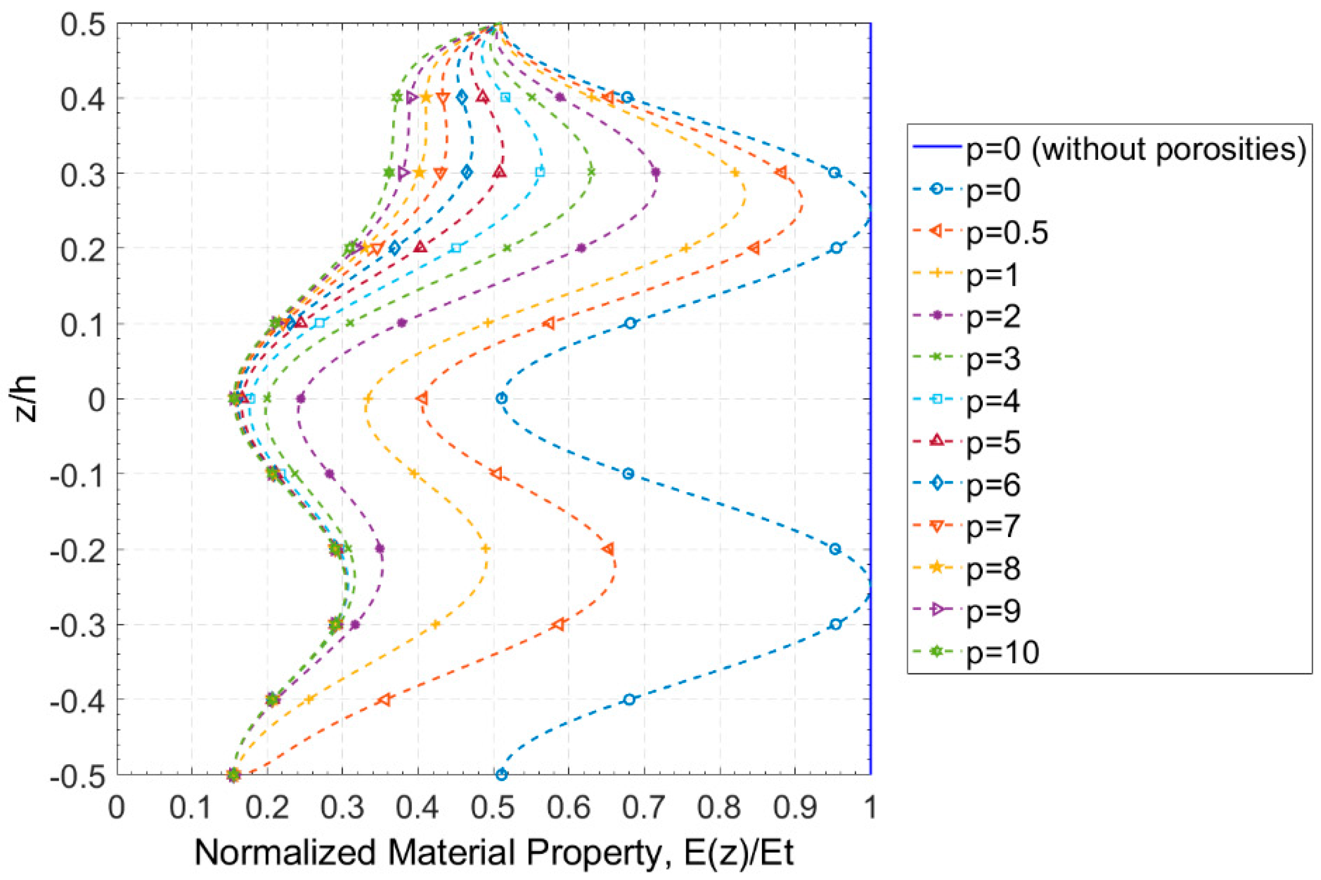
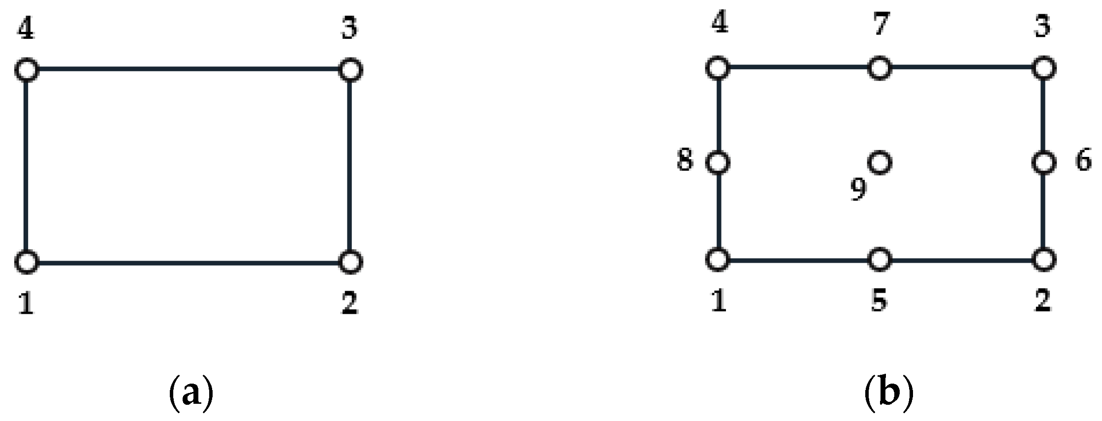
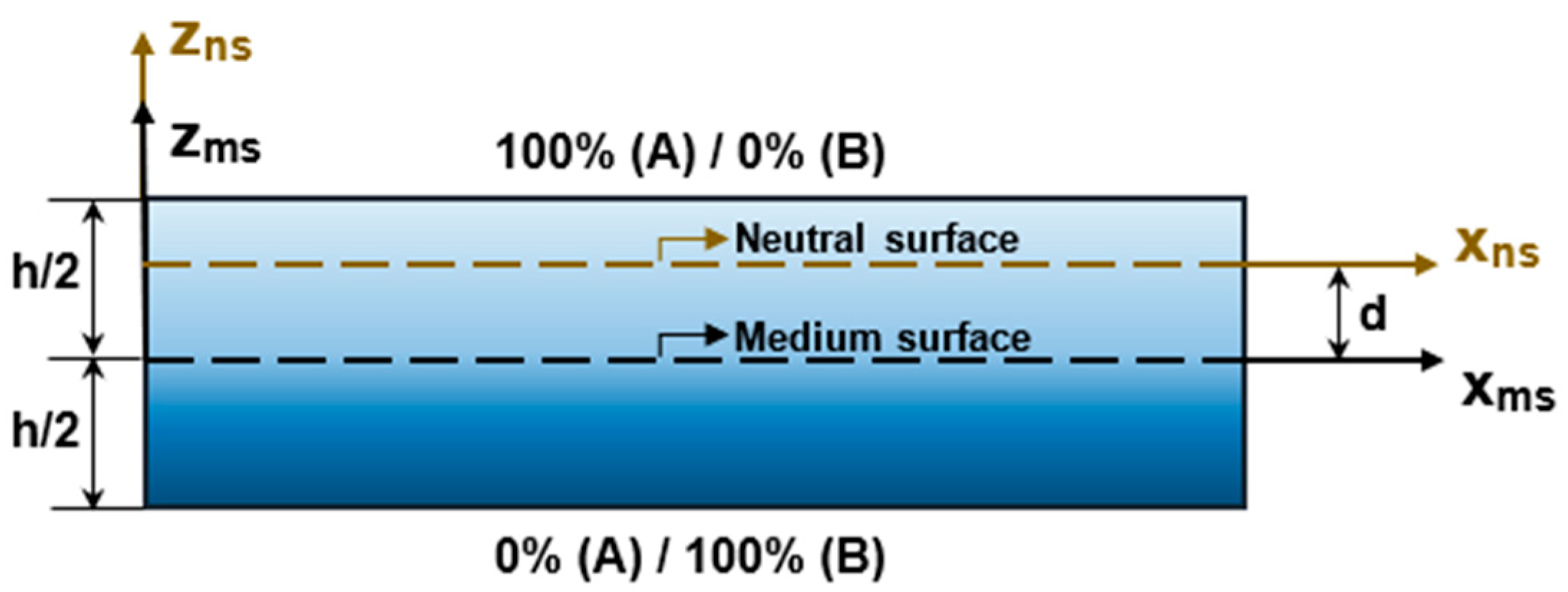
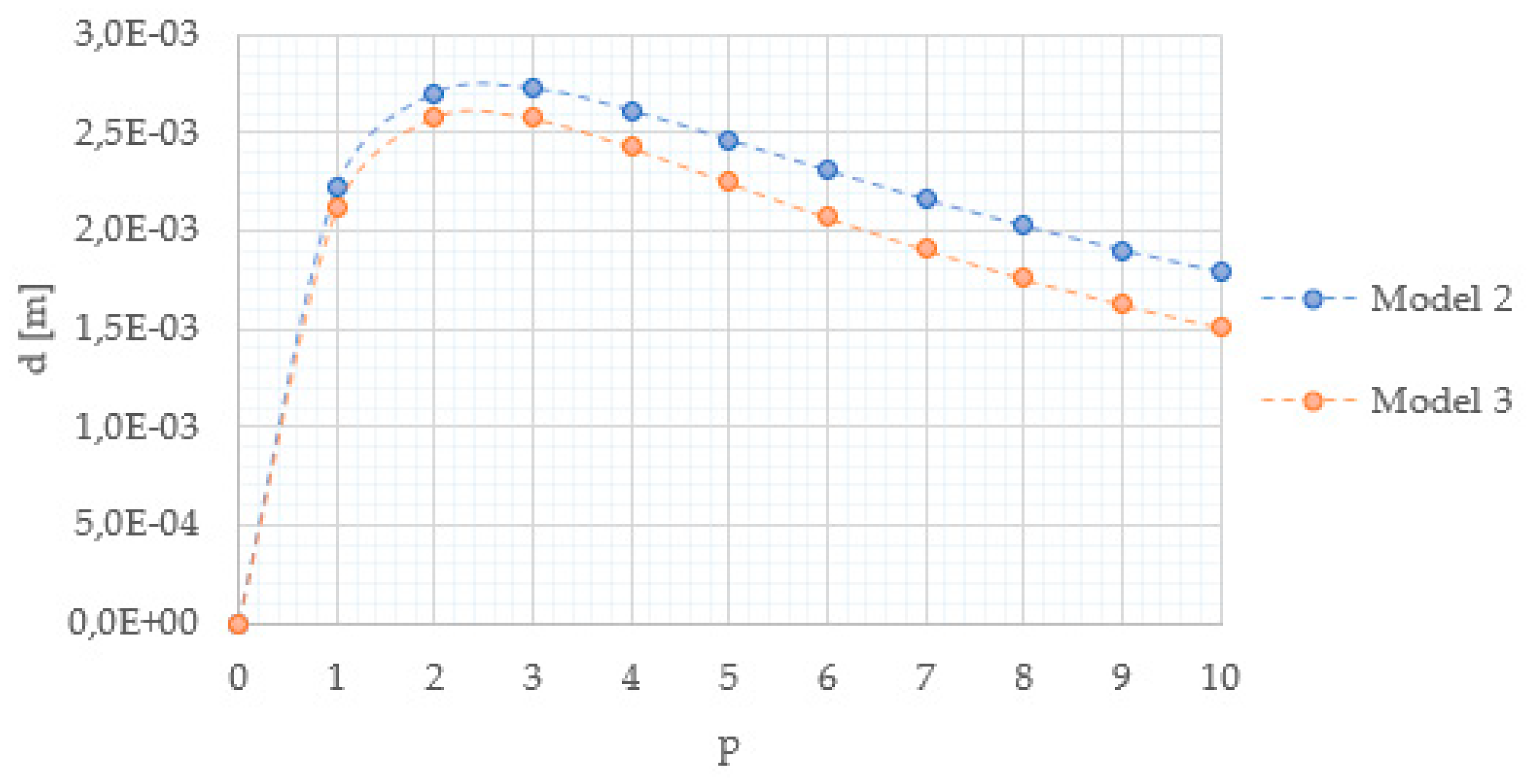
Hence, the present work presents three porosity distribution models, two of which are based on the reference literature, and respective estimates of material properties. For these cases, we performed a set of parametric studies focused on the static behavior of porous plates with a functional gradient in order to characterize the influence of the shear correction factor, associated with the use of the first-order shear deformation theory. These studies were performed via the finite element method considering an equivalent single layer approach. To the best of our knowledge, there are no previously published works focusing on the assessment of the influence of the shear correction factor in the static bending behavior of porous plates. Hence, this study addresses this, considering the characterization of the neutral surface deviation from the mid-plane surface, which also provides an illustrative measure of the medium’s heterogeneity, typical of graded mixture and porous materials.

2. Materials and Methods

Considering the wide and varied number of applications of porous materials briefly discussed in the introductory section, the prediction of their mechanical properties is very relevant. Several models to predict the Young modulus of porous materials have recently been proposed, including linear, quadratic, and exponential models, although these are not suitable for porosities which are too low or too high [29]. Carranza et al. evaluated the Young modulus of metallic foams with fractal porosity distribution, and the respective estimates were close to the experimental results. In this way, they proved the expected effect, and verified that the appropriate choice of the porosity distribution model is an important factor [38].

2.1. Functionally Graded Materials

The flexibility in tailoring material properties makes FGMs very interesting for many applications in diverse engineering and science fields like bioengineering, mechanics, and aerospace.

The procedures for manufacturing FGMs are designed in order to obtain a specific spatial distribution of the constitutive phases. The continuous and gradual spatial distribution is responsible for the unique morphology and properties of these materials that make them stand out from others [1]. The gradual evolution of the phases can be varied, and there may even be different variations in more than one direction in the same FGM [2]. Figure 1 illustrates one example of material distribution though one direction of a dual-phase FGM.

As a consequence of the gradual evolution of the bulk fractions and microstructure of FGMs, the respective macroscopic properties also present gradual changes. The gradual evolution of the material properties characteristic of FGMs makes it possible to design them in order to achieve specific mechanical, physical, or biological properties [1]. Since the volume fraction of the constituent phases can vary gradually in one or more directions, the present work considers the particular case of a dual-phase FGM plate in which this variation occurs in one only direction—specifically the thickness direction, as in [42]. In this case, the evolution of the volume fraction according to the direction of the z axis occurs according to the following power law:

$$V_f={\left(\frac{z}{h}+\frac{1}{2}\right)}^p,$$

(1)

where h and z represent, respectively, the plate’s thickness and the thickness coordinate, where the origin corresponds to the FGM plate’s middle surface, thus z ∈ [−h/2, h/2]. Representing this material distribution, Figure 2 presents the volume fraction evolution through the thickness for some power law exponent values. As can be seen, the exponent p dictates the volume fraction behavior along the plate’s thickness.

As the volume fraction of the phases of the constituents of FGMs is a function of the z coordinate, so too are the corresponding material properties. The effective material properties of an FGM can be estimated by the Voigt rule of mixtures, according to:

$$P_{FGM}=(P_t-P_b)V_{f_t}+P_b$$

(2)

where P_FGM is the FGM property, and P_t and P_b represent the corresponding property at top and bottom surfaces, respectively. This approach is suitable for FGMs whose phases are not very different from each other [43].

2.2. Porosity Distributions

Functionally graded porous materials combine characteristics of both FGMs and porous materials. Beyond the great rigidity–weight ratio, the incomparable mechanical properties they present explains why these distinctive materials are widely used in a wide range of diverse fields [44].

Despite great developments in manufacturing processes, the formation of micro-voids or porosities is still a fact [4], and in some specific applications this can be even desirable and designed for. Regardless of the specific case, as a consequence of these pores, the material’s strength will become lower, and this should be included in mechanical behavior studies [44].

The present work considers three types of porosity distributions through the thickness, the first one being proposed by Kim et al. [45] and applied in several studies, such as those developed by Coskun et al. [46] and by Li and Zheng [22]. The last two were inspired in the uniform distribution mentioned by Du et al. [47], whose studies focus on open-cell metal foams rectangular plates considering different porosity distributions through the thickness.

• Porosity Model M1:

Concerning porous FGMs, Kim et al. [45] considered, among other things, a porosity distribution through the thickness given by:

$$\Phi \left(z\right)=\varphi cos\left[\frac{\pi }{2}\left(\frac{z}{h}-\frac{1}{2}\right)\right],$$

(3)

where $z$ represents the thickness coordinate, $h$ represents the plate’s thickness, and ϕ is the maximum porosity value.

Thus, the rule of mixtures is affected by this distribution and the effective Young modulus (E) and Poisson’s ratio (υ) can be estimated as follows:

$$E\left(z\right)=\left[\left(E_t-E_b\right){\left(\frac{z}{h}+\frac{1}{2}\right)}^p+E_b\right]\left(1-\Phi \left(z\right)\right),$$

(4)

$$\upsilon \left(z\right)=\left[\left({\upsilon }_t-{\upsilon }_b\right){\left(\frac{z}{h}+\frac{1}{2}\right)}^p+{\upsilon }_b\right]\left(1-\Phi \left(z\right)\right).$$

(5)

In both Equations (4) and (5), the indexes t and b indicate the top and bottom surfaces, respectively.

Figure 3 illustrates, in a normalized form, the porosity distribution through the thickness, showing an evolution from an absence of pores in the bottom surface to a maximum porosity in the top surface, and the normalized Young’s modulus evolution through the thickness for different maximum porosity values and power law exponents, elucidating how this model of porosity distribution affects this material property.

The next two porosity distribution models were based on the uniform distribution referred to in [47].

In both models, the porosity coefficient ($e_0$) is given by Equation (6), and parameter β can be calculated through the relation in Equation (7).

$$e_0=1-\frac{E_b}{E_t},$$

(6)

$$\beta =\frac{1}{e_0}-\frac{1}{e_0}{\left(\frac{2}{\pi }\sqrt{1-e_0}-\frac{2}{\pi }+1\right)}^2,$$

(7)

• Porosity Model M2:

In this model, the material properties, namely Young’s modulus and Poisson’s ratio, are estimated by Equations (8) and (9), and the graph of the evolution of the normalized Young modulus through the thickness is presented in Figure 4.

$$E\left(z\right)=\left[\left(E_t-E_b\right){\left(\frac{z}{h}+\frac{1}{2}\right)}^p+E_b\right]\left(1-e_0\beta \right),$$

(8)

$$\upsilon \left(z\right)=\left[\left({\upsilon }_t-{\upsilon }_b\right){\left(\frac{z}{h}+\frac{1}{2}\right)}^p+{\upsilon }_b\right]\left(1-e_0\beta \right).$$

(9)

• Porosity Model M3:

This model introduces to the previous one a porosity gradient through the thickness, with the respective effective materials properties being given by:

$$E\left(z\right)=\left[\left(E_t-E_b\right){\left(\frac{z}{h}+\frac{1}{2}\right)}^p+E_b\right]\left[1-e_0\beta co{s}^2\left(2\pi \frac{z}{h}\right)\right],$$

(10)

$$\upsilon \left(z\right)=\left[\left({\upsilon }_t-{\upsilon }_b\right){\left(\frac{z}{h}+\frac{1}{2}\right)}^p+{\upsilon }_b\right]\left[1-e_0\beta co{s}^2\left(2\pi \frac{z}{h}\right)\right].$$

(11)

Figure 5 shows the variation of the normalized Young’s modulus through the thickness. Note that the porosity distribution fluctuates between maxima and minima along the thickness.

Note that on the upper surface the normalized Young’s modulus takes the same value for all power law exponents evaluated once the equality $E\left(z\right)=E_t\left(1-e_0\beta \right)$ is verified. On the opposite surface, Young’s modulus is given by $E\left(z\right)=E_b\left(1-e_0\beta \right)$, which justifies the fact that the corresponding p = 0 curve constitutes an exception from the others, since this particular case corresponds to a plate made up of a single phase whose Young’s modulus is given by E_t, while in the remaining cases the bottom face corresponds to the phase with Young’s modulus given by E_b.

In all three porosity distribution models, the shear modulus is estimated by:

$$G\left(z\right)=\frac{E\left(z\right)}{2\left(1+\upsilon \left(z\right)\right)}.$$

(12)

In Figure 3b, Figure 4 and Figure 5, the curve corresponding to the case of null power law exponent without porosity is also presented. In this case the represented material property is given by Equation (2), taking the value of $E_t$. Thus, the corresponding normalized form takes the value 1 through the entire plate thickness.

2.3. Constitutive Relation and Finite Element Models

The static behavior of porous plates with functional classification was evaluated for a set of studies through finite element analysis based on the first-order shear deformation theory (FSDT) and on third-order shear deformation theory (HSDT). According to FSDT the displacement field can be described by:

$$u\left(x,y,z\right)=u^0\left(x,y\right)+z·{\theta }_x^0\left(x,y\right),$$

$$v\left(x,y,z\right)=v^0\left(x,y\right)+z·{\theta }_y^0\left(x,y\right),$$

(13)

$$w\left(x,y,z\right)=w^0\left(x,y\right),$$

where u(x,y,z), v(x,y,z), and w(x,y,z) are the displacements of a certain plate coordinate point, and u⁰(x,y), v⁰(x,y) and w⁰(x,y) represent the displacements of a mid-plane point associated to them. The normals to the mid-plane rotations are represented by ${\theta }_x^0$ and ${\theta }_y^0$, respectively. Thus, this model considers a total of five degrees of freedom per node, $q=\left[u^0,v^0,w^0,{\theta }_x^0,{\theta }_y^0\right].$ Considering small deformations, the elasticity kinematic relation leads to the following strain field, omitting dependencies for simplicity reasons:

${\epsilon }_x={\epsilon }_x^0+\mathrm{z}·k_x^0$ ${\epsilon }_y={\epsilon }_y^0+\mathrm{z}·k_y^0$ ${\gamma }_{xy}={\gamma }_{xy}^0+z·k_{xy}^0$		${\gamma }_{xz}={\gamma }_{xz}^0$ ${\gamma }_{yz}={\gamma }_{yz}^0$	(14)
${\epsilon }_x^0=\frac{\partial u^0}{\partial x}$ ${\epsilon }_y^0=\frac{\partial v^0}{\partial y}$ ${\gamma }_{xy}^0=\frac{\partial u^0}{\partial y}+\frac{\partial v^0}{\partial x}$	$k_x^0=\frac{\partial {\theta }_x^0}{\partial x}$ $k_y^0=\frac{\partial {\theta }_y^0}{\partial y}$ $k_{xy}^0=\frac{\partial {\theta }_y^0}{\partial x}+\frac{\partial {\theta }_x^0}{\partial y}$	${\gamma }_{xz}^0={\theta }_x^0+\frac{\partial w^0}{\partial x}$ ${\gamma }_{yz}^0={\theta }_y^0+\frac{\partial w^0}{\partial y}$

where ε_x, ε_y, and γ_xy correspond to the two in-plane normal strains and to the in-plane total shear strain, respectively. The interlaminar transverse shear strains are represented by γ_yz and γ_xz. This strain field is characterized by a null normal transverse strain (${\epsilon }_z=0$), denoting thickness inextensibility. Since the FGM considered in the studies carried out can be considered as an isotropic material, the constitutive law governing the relationship between the stress and strain fields is given by:

$$\left[\begin{array}{c}{\sigma }_x\\ {\sigma }_y\\ {\sigma }_{xy}\\ {\sigma }_{yz}\\ {\sigma }_{xz}\end{array}\right]=\left[\begin{array}{ccccc}{Q}_{11}& Q_{12}& 0& 0& 0\\ Q_{12}& Q_{22}& 0& 0& 0\\ 0& 0& Q_{66}& 0& 0\\ 0& 0& 0& k·Q_{44}& 0\\ 0& 0& 0& 0& k·Q_{55}\end{array}\right]·\left[\begin{array}{c}{\epsilon }_x\\ {\epsilon }_y\\ {\gamma }_{xy}\\ {\gamma }_{yz}\\ {\gamma }_{xz}\end{array}\right].$$

(15)

The coefficients $Q_{\mathrm{ij}}$, provided by [48], stand for the elastic coefficients, which in the present work depend on the z coordinate due to the variation in material properties through the thickness direction:

$$\begin{gathered} Q_{11}=Q_{22}=\frac{E_{FGM}\left(z\right)}{1-{\upsilon }_{FGM}^2\left(z\right)} \\ {Q}_{12}=\frac{{\upsilon }_{FGM}\left(z\right)·E_{FGM}\left(z\right)}{1-{\upsilon }_{FGM}^2\left(z\right)}, \\ {Q}_{44}=Q_{55}=Q_{66}=G_{FGM}\left(z\right). \end{gathered}$$

(16)

The HSDT displacement field also considered in this work for comparison purposes was proposed by Kant et al. [49], and is given by:

$$u\left(x,y,z\right)=u^0\left(x,y\right)+z·{\theta }_x^0\left(x,y\right)+z^3·{\theta }_x^{*}\left(x,y\right),$$

$$v\left(x,y,z\right)=v^0\left(x,y\right)+z·{\theta }_y^0\left(x,y\right)+z^3·{\theta }_y^{*}\left(x,y\right),$$

(17)

$$w\left(x,y,z\right)=w^0\left(x,y\right)+z^2·w^{*}\left(x,y\right).$$

As can be observed, this higher-order displacement field not only allows for in-plane displacements that vary as cubic functions of the thickness coordinate, but it also allows for thickness extensibility. This higher-order theory was implemented for comparison purposes, but was not the main focus of the present work.

The finite element method was used for the study presented in this work. This method is widely used due to its great versatility, able to solve a wide range of physical problems ruled by differential equations. In this numerical method, the domain of a certain problem is discretized into elementary subdomains, which obey continuity and equilibrium requirements between adjacent subdomains. The resolution of a problem by the finite element method can generically be described by three steps [49,50], as follows. After the pre-processing stage, where all aspects related to the domain discretization and topology, material and geometrical characteristics, loading and boundary conditions are accomplished, one proceeds to the analysis phase where the intended analysis is performed and primary variables are obtained. The results of this analysis can then be post-processed in order to obtain other derived physical quantities of interest in the third and final phase of this method. The plates analyzed in the present work had a rectangular geometry configuration (Figure 6) with a graded material distribution, as already mentioned.

Taking into consideration their geometry, the plates were discretized into quadrilateral finite elements. To enable a more comprehensive study, we considered bilinear and biquadratic quadrilateral plate finite elements from the Lagrange family, as illustrated in Figure 7. The bilinear element (a) contained one node at each vertex (four nodes in total), while the biquadratic element (b) additionally contained a center node and one node at the midpoint of each side, resulting in a total of nine nodes. Each node possessed five degrees of freedom—three translations and two rotations associated to the plate mid-plane, as previously mentioned.

As the main aim of the present work is related to the assessment of the influence of the shear correction factor on the static bending of FGP plates, the procedure considered to achieve the global equilibrium equations to be solved was based on the minimization of the plates’ potential energy. This mathematical formulation yields for each element a set of equilibrium equations. Considering the whole discretized domain where continuity and equilibrium aspects ensure the discretized model will be representative, we finally obtain the global equilibrium equation:

$${\left\{f\right\}}^{global}={\left[K\right]}^{global}·{\left\{u\right\}}^{global},$$

(18)

where ${\left\{u\right\}}^{global}$ denotes the problem solution (i.e., the generalized nodal displacements), ${\left\{f\right\}}^{global}$ represents the generalized forces applied to the plates, and ${\left[K\right]}^{global}$ is the global stiffness matrix. The solution of the problem is obtained after the imposition of the plates’ boundary conditions.

2.4. Shear Correction Factor

The studies developed in this work are based on FSDT, which requires the introduction of a shear correction factor on the transverse shear components of the elastic stiffness coefficients matrix in order to redress the uniform transverse shear stresses/strains arising from the deformation kinematics based on the displacement field. Despite this need, FSDT-based models continue to be widely used in the modeling of structures, due to their lower computational cost when compared to other theories and also due to their applicability domain. It is possible to conclude that, even considering a bilinear element, results were very good when compared to other authors’ alternative solutions and with biquadratic elements, while also having a lower computational cost. Regarding the homogeneous plates, the shear correction value considered was 5/6. However, the overall heterogeneity of FGMs due to the gradual evolution of their properties makes it desirable to calculate the correction factor for each specific case [6,43,51].

Shear correction factors determined through predictor–corrector procedures that use iteration processes depend on plate geometry, as well as boundary and load conditions. Therefore, the factors thus determined are limited to a given system and cannot be applied to different configurations. The use of energy considerations for the calculation of shear correction coefficients is quite common in studies involving laminated composite materials and FGMs [51]. Nguyen et al. [51] worked on this subject concerning FGMs, comparing the strain energies obtained from the average shear stresses and from the equilibrium to calculate the shear correction factors. Efraim and Eisenberg developed a shear correction factor depending on Poisson’s ratio and the volume fractions of both material phases present in a functionally graded plate [52]. Working on FGPs, Li et al. [53] calculated the shear correction factor as a function of the power law exponent, thickness-to-length ratio (a/h), and of some constant coefficients that depend on the material phases involved.

The shear correction factor used in the present work (here represented by k) was estimated using a formulation similar to the one used by Singha et al. [54]. Accordingly, the reference surface used for the shear correction factor calculation was the neutral one and not the mid-surface as usual. To this purpose we considered an FGP with thickness h as illustrated in Figure 8, where z_ms and z_ns are the coordinates of a point in the thickness direction relative to the medium and neutral surfaces, respectively.

According to this formulation, the shift of the neutral surface (d) is given by:

$$d=\frac{{{\displaystyle \int }}_{-h/2}^{h/2}E\left(z_{ms}\right)·z_{ms}d{z}_{ms}}{{{\displaystyle \int }}_{-h/2}^{h/2}E\left(z_{ms}\right)d{z}_{ms}}.$$

(19)

The shear correction factor is then derived from the equivalent energy principle, and can be determined by Equation (20) [54]:

$$k=\frac{{\left({{\displaystyle \int }}_{-\frac{h}{2}-d}^{\frac{h}{2}-d}\left({{\displaystyle \int }}_{-\frac{h}{2}-d}^{z_{ns}}E\left(\xi \right)·\xi d\xi \right)d{z}_{ns}\right)}^2}{{{\displaystyle \int }}_{-\frac{h}{2}-d}^{z_{ns}}{\overline{Q}}_{55}d{z}_{ns}·{{\displaystyle \int }}_{-\frac{h}{2}-d}^{\frac{h}{2}-d}\frac{{\left({{\displaystyle \int }}_{-\frac{h}{2}-d}^{z_{ns}}E\left(\xi \right)·\xi d\xi \right)}^2}{G\left(z_{ns}\right)}}.$$

(20)

As applied to determine shear correction factor, all calculations carried out a posteriori were simply affected by a referential translation according to the coordinate vector (0, 0, −d).

3. Results

The present section, dedicated to the presentation of results and their preliminary discussion, comprises a first verification study, after which a set of case studies considering different porosity distributions models are presented and analyzed concerning their influence on neutral surface shift, shear correction factor, and maximum transverse displacement.

3.1. Verification Studies

3.1.1. Shear Correction Factor

In the course of the literature review, no studies were found on the correction factor in the context of FGMs considering porosity distributions. For this reason, this first verification study regarding the approach applied to the correction factor determination was carried out considering a metal/ceramic functionally graded plate where the volume fraction of the ceramic phase is given by Equation (1). To this purpose, a square plate with unitary length and aspect ratio of 100 was considered, according to [43]. The results obtained for different power law exponents and Young’s modulus ratios between both ceramic and metallic phases are presented in

Table 1. Shear correction factor for different material parameters.

p	${\mathit{E}}_{\mathit{c}}/{\mathit{E}}_{\mathit{m}}$
	1		2		4		6
	k[43]	$k$	k[43]	k	k[43]	k	k[43]	k
0	5/6	0.8333	5/6	0.8333	5/6	0.8333	5/6	0.8333
1	5/6	0.8333	0.8320	0.8320	0.8305	0.8305	0.8305	0.8305
2	5/6	0.8333	0.8095	0.8095	0.7804	0.7804	0.7662	0.7662
5	5/6	0.8333	0.7891	0.7891	0.7175	0.7175	0.6643	0.6641
10	5/6	0.8333	0.7989	0.7989	0.7316	0.7318	0.6743	0.6746
p	${\mathit{E}}_{\mathit{c}}/{\mathit{E}}_{\mathit{m}}$
	8		10		15		20
	k[43]	$k$	k[43]	k	k[43]	k	k[43]	k
0	5/6	0.8333	5/6	0.8333	5/6	0.8333	5/6	0.8333
1	0.8308	0.8308	0.8312	0.8312	0.8319	0.8319	0.8323	0.8323
2	0.7593	0.7594	0.7563	0.7563	0.7555	0.7556	0.758	0.7580
5	0.6238	0.6235	0.5923	0.5919	0.5381	0.5377	0.5046	0.5043
10	0.6262	0.6266	0.5856	0.5860	0.5073	0.5080	0.4513	0.4521

, showing an excellent agreement with the reference results for all parameter values considered.

3.1.2. Porosity Distribution Model 1 (M1)

The first porosity model (M1) was submitted to verification studies. For this, and according to reference [6], an FGM square plate with 17.6 μm thickness and an aspect ratio of 20 was considered. Regarding the constituent materials, the Young moduli of the top and bottom surfaces were assumed to be E_t = 14.4 GPa and E_b = 1.44 GPa respectively, and in this particular study, the Poisson ratio was considered constant, assuming the value of 0.38. The plate, simply supported, was considered under a uniformly distributed load with 100 kPa magnitude and was discretized in a 10 × 10 mesh of four node finite elements (Q4).

The normalized transverse displacement and the respective relative deviation to the reference, presented in

Table 2. Results of the porosity distribution model 1 (M1) verification study.

p	ϕ	$\overline{\mathit{w}}$	δ (%)
0	0	4.220 × 10−3	1.49
	0.2	4.798 × 10−3	0.43
	0.5	6.242 × 10−3	−0.57
1	0.5	1.452 × 10−2	0.26
5	0.5	2.685 × 10−2	−0.18

, were obtained by Equations (21) and (22), respectively.

$$\overline{w}=\frac{E_b·h^3}{q_0·a^4}w\left(\frac{a}{2},\frac{b}{2},0\right),$$

(21)

$$\delta (\%)=\frac{{\overline{w}}^{present}-{\overline{w}}^{reference}}{{\overline{w}}^{reference}}·100(\%).$$

(22)

The small relative deviations observed make it possible to conclude that there is very good agreement between the present model and the reference results, although a different approach was applied. In particular, the higher relative deviation occurs when considering an isotropic homogeneous material without porosities (p = 0, ϕ = 0).

3.2. Case Studies

In order to perform a set of parametric studies relevant for this work’s objectives, we carried out simulations on a set of case studies, in which FGM square plates with 25 mm thickness and aspect ratio 20 were considered. The material properties involved in the studies presented in this section are given in

Table 3. Material properties.

Material	Young’s Modulus (GPa)	Poisson’s Ratio
Aluminum (Al)	70	0.33
Titanium Oxide (TiO2)	230	0.27

, and the volume fraction of TiO₂ is given by Equation (1). The plates were considered simply supported and submitted to a uniform load with 100 kPa of magnitude.

The case studies show the influence of the different porosity distribution models in the neutral surface shift, shear correction factor, and maximum transverse displacement for a range of power law exponents. The influence of finite element type used was also studied.

3.2.1. Influence on Neutral Surface Shift and Shear Correction Factor

In this subsection we present the studies performed to explore the effects of the porosity distribution on the neutral surface shift and shear correction factor.

• Porosity Distribution Model 1 (M1):

When considering porosities distributed according to model M1, it is important to evaluate how the maximum porosity value combined with the power law exponent affects the neutral surface shift and the shear correction factor. For this purpose, the following sets of values were respectively considered for the maximum porosity value and for the exponent of the power law: $\varphi =\left\{0,0.1,0.2,0.3,0.4,0.5,0.6\right\}$ and $p=\left\{0,1,2,5,10\right\}$. The results obtained are presented in

Table 4. Porosities distribution M1: neutral surface’ shift and shear correction factor.

ϕ	p	d (m)	d/h	k
0	0	0	0	5/6
	1	2.2222 × 10−3	0.0889	0.8279
	2	2.7027 × 10−3	0.1081	0.7828
	5	2.4631 × 10−3	0.0985	0.7344
	10	1.7921 × 10−3	0.0717	0.7499
0.1	0	−2.3222 × 10−4	−0.0093	0.8316
	1	2.0233 × 10−3	0.0809	0.8289
	2	2.4955 × 10−3	0.0998	0.7843
	5	2.2257 × 10−3	0.0890	0.7359
	10	1.5422 × 10−3	0.0617	0.7505
0.2	0	−4.9832 × 10−4	−0.0199	0.8297
	1	1.7903 × 10−3	0.0716	0.8304
	2	2.2520 × 10−3	0.0901	0.7865
	5	1.9481 × 10−3	0.0779	0.7378
	10	1.2519 × 10−3	0.0501	0.7513
0.3	0	−8.0630 × 10−4	−0.0323	0.8275
	1	1.5138 × 10−3	0.0606	0.8325
	2	1.9620 × 10−3	0.0785	0.7894
	5	1.6190 × 10−3	0.0648	0.7403
	10	9.1039 × 10−4	0.0364	0.7522
0.4	0	−1.1669 × 10−3	−0.0467	0.8248
	1	1.1805 × 10−3	0.0472	0.8353
	2	1.6107 × 10−3	0.0644	0.7934
	5	1.2227 × 10−3	0.0489	0.7436
	10	5.0299 × 10−4	0.0201	0.7534
0.5	0	−1.5948 × 10−3	−0.0638	0.8217
	1	7.7050 × 10−4	0.0308	0.8390
	2	1.1761 × 10−3	0.0470	0.7988
	5	7.3631 × 10−4	0.0295	0.7477
	10	8.5279 × 10−6	0.0003	0.7546
0.6	0	2.1109 × 10−3	0.0844	0.8177
	1	2.5421 × 10−4	0.0102	0.8439
	2	6.2495 × 10−4	0.0250	0.8059
	5	1.2505 × 10−4	0.0050	0.7529
	10	−6.0425 × 10−4	−0.0242	0.7560

, Figure 9 and Figure 10.

Independent of the ϕ value, the neutral surface shift increased from p = 0 to p = 2, where it had its maximum value, then decreasing from p = 2 to p = 10. Additionally, for all maximum porosity values considered, except for the case where $\varphi =0.6$, the shear correction factor decreased for power law exponents between 0 and 5, increasing for the last transition from p = 5 to p = 10. This is explained by the fact that, for higher values of the power law exponent, the functionally graded plate approaches a homogeneous isotropic composition, and at the limit where p tends to infinity, the plate will consist of a single phase (aluminum in this case), so the value of the shear correction factor tends to the typical value 5/6.

When the maximum porosities took the values 0 or 0.1, the shear correction factor decreased from p = 0 to p = 5, increasing for higher values of power law exponent. For the remaining values of maximum porosities this factor increased in the transition from p = 0 to p = 1, decreased from p = 1 to p = 5, and increased again until p = 10.

In the case of an isotropic homogeneous plate (p = 0), the shear correction factor decreased when the maximum porosity values increased. This was also true for the neutral surface shift, excepting for the abrupt increase in the transition between ϕ = 0.5 and ϕ = 0.6. For other power law exponents, as the maximum porosity values increased the neutral surface shift decreased and the shear correction factor increased.

• Porosity Distribution Models 2 and 3 (M2 and M3):

Concerning these models, we evaluated the influence of the power law exponent, taking the set of integers from 0 to 10. Figure 11 and Figure 12 show the evolution of neutral surface shift and shear correction factor, respectively, for both distribution models M2 and M3. The curves show a neutral surface shift behavior similar to the one observed in the previous study and a shear correction factor with a decreasing behavior up to p = 5, after which it increased with the exponent of the power law. This behavior was similar in both models. The porosity distribution M3 led to smaller neutral surface shifts, and the difference between both models increased with increasing power law exponent.

The porosity distribution model M3 generated lower values for the shear correction factor, with the difference between the two models decreasing with the increase in the power law exponent, as opposed to what was observed for the neutral surface shift.

3.2.2. Influence on Absolute Maximum Transverse Displacement

In the studies presented in this section, the absolute maximum transverse displacement corresponds to the magnitude of the plate’s center displacement given the considered boundary and load conditions. The results include both 4-node (Q4) and 9-node (Q9) plate finite element results, using the calculated shear correction factor (Section 2.4) here denoted by $k^{calc}$ and the often used value of 5/6. The relative deviations presented were determined by the following equations:

$${\delta }_{Q_4}(\%)=\frac{w_{\left(k=\frac{5}{6}\right)}^{Q_4}-w_{\left(k^{calc}\right)}^{Q_4}}{w_{\left(k^{calc}\right)}^{Q_4}}·100(\%),$$

(23)

$${\delta }_{Q_9}(\%)=\frac{w_{\left(k=\frac{5}{6}\right)}^{Q_9}-w_{\left(k^{calc}\right)}^{Q_9}}{w_{\left(k^{calc}\right)}^{Q_9}}·100(\%).$$

(24)

In the convergence study presented for porosity distribution model 1, the relative deviations were determined by Equation (25), where the index $i$ denotes the order of the data in the respective results table.

$${\delta }_{mesh}(\%)=\frac{w_i-w_{i-1}}{w_{i-1}}·100(\%),i\ge 2$$

(25)

• Porosity Distribution Model 1 (M1):

We developed convergence studies in order to evidence the reason for the discretization selection. To illustrate them, we present the results obtained for two sets of distinct parameterizations of maximum porosities and power law exponent values, considering Q4 finite elements and FSDT. The results achieved and presented in

Table 5. Porosity distribution model M1: convergence study.

ϕ	p	Mesh	$\mathit{w}\left(\frac{\mathit{a}}{2},\frac{\mathit{b}}{2},0\right)\left(\mathbf{m}\right)$	${\mathit{\delta }}_{\mathit{m}\mathit{e}\mathit{s}\mathit{h}}(\%)$
0.1	1	4 × 4	−1.3855 × 10−4	-
		6 × 6	−1.4035 × 10−4	1.30
		8 × 8	−1.4091 × 10−4	0.39
		10 × 10	−1.4116 × 10−4	0.18
		12 × 12	−1.4129 × 10−4	0.10
		14 × 14	−1.4137 × 10−4	0.06
		16 × 16	−1.4142 × 10−4	0.04
		18 × 18	−1.4146 × 10−4	0.03
		20 × 20	−1.4149 × 10−4	0.02
0.5	5	4 × 4	−2.5263 × 10−4	-
		6 × 6	−2.5597 × 10−4	1.32
		8 × 8	−2.5701 × 10−4	0.40
		10 × 10	−2.5747 × 10−4	0.18
		12 × 12	−2.5773 × 10−4	0.10
		14 × 14	−2.5788 × 10−4	0.06
		16 × 16	−2.5798 × 10−4	0.04
		18 × 18	−2.5804 × 10−4	0.03
		20 × 20	−2.5809 × 10−4	0.02

show that the mesh refinement from 10 × 10 elements presents a deviation of less than 0.2%. Based on this evidence, the following studies were performed considering a mesh of 10 × 10 elements.

The results obtained regarding transverse displacement at the plate’s center are presented in

Table 6. Porosity distribution model M1: plates center transverse displacement for different finite models and shear correction factor approaches.

ϕ	p	Q4		Q9
		${\mathit{k}}^{\mathit{c}\mathit{a}\mathit{l}\mathit{c}}$	$\mathit{k}=5/6$	${\mathit{k}}^{\mathit{c}\mathit{a}\mathit{l}\mathit{c}}$	$\mathit{k}=5/6$
		$\mathit{w}\left(\frac{\mathit{a}}{2},\frac{\mathit{b}}{2},0\right)\left(\mathbf{m}\right)$	${\mathit{\delta }}_{\mathit{Q}4}(\%)$	$\mathit{w}\left(\frac{\mathit{a}}{2},\frac{\mathit{b}}{2},0\right)\left(\mathbf{m}\right)$	${\mathit{\delta }}_{\mathit{Q}9}(\%)$
0	0	−7.9330 × 10−5	0.00	−7.9625 × 10−5	0.00
	1	−1.3168 × 10−4	−5.14	−1.3215 × 10−4	−4.96
	2	−1.5267 × 10−4	−7.17	−1.5321 × 10−4	−6.94
	5	−1.7054 × 10−4	−5.51	−1.7114 × 10−4	−5.33
	10	−1.8510 × 10−4	−2.95	−1.8574 × 10−4	−2.85
0.3	0	−9.9540 × 10−5	−0.94	−9.9930 × 10−5	−0.93
	1	−1.6493 × 10−4	−1.81	−1.6556 × 10−4	−1.70
	2	−1.9003 × 10−4	−3.06	−1.9075 × 10−4	−2.91
	5	−2.1256 × 10−4	−1.83	−2.1335 × 10−4	−1.73
	10	−2.3281 × 10−4	−0.50	−2.3367 × 10−4	−0.46
0.6	0	−1.3788 × 10−4	−5.65	−1.3845 × 10−4	−5.55
	1	−2.2603 × 10−4	0.13	−2.2695 × 10−4	0.14
	2	−2.5832 × 10−4	0.03	−2.5936 × 10−4	0.07
	5	−2.9115 × 10−4	−0.07	−2.9231 × 10−4	−0.06
	10	−3.2350 × 10−4	−0.91	−3.2479 × 10−4	−0.91

. In this study, the displacement increased with increasing maximum porosity for all power law exponents considered, as expected.

Comparing the results with 4-node elements and different shear correction factor approaches, the relative deviation increased from p = 0 to p = 2, decreasing with increasing power law exponents. Moreover, the increase in maximum porosity value resulted in a relative deviation increase for p = 0—the opposite behavior to that verified for the intermediate power law exponents. When considering p = 10, the relative deviations showed an oscillating behavior with increasing maximum porosity value. However, for maximum porosity values of 0.5 and 0.6 and intermediate power law exponents these deviations were nearly zero, except for the case of null power law exponent. The same behavior was verified when doing the same comparative study with 9-node elements, except for the specific case considering a maximum porosity value of 0.6.

Additionally, we verified that when considering the common value of 5/6 for the shear correction factor, the relative deviation between the results observed for Q4 and Q9 elements was very low, presenting a decreasing behavior with increasing maximum porosity value, except for p = 0, where the opposite was verified. With the other approach, this relative deviation also presented very low values, although the increase of maximum porosity value resulted in higher deviations for all power law exponents considered.

Figure 13 shows the plate’s center displacement for different power law exponents and maximum porosity values, obtained considering Q4 finite elements. In the figure, it is clear that higher maximum porosity values corresponded to higher maximum transverse displacement magnitudes for all exponents, with the effect being more pronounced when considering larger exponents.

In order to compare the results obtained by applying different shear deformation theories, keeping the configurations considered above, the plate’s center displacement was determined by applying the third-order shear deformation theory (HSDT) proposed by [49], and also implemented by the authors for this purpose. The results obtained are presented in

Table 7. Porosity distribution model M1: plate’s center transverse displacement for different shear deformation theories.

ϕ	p	${\mathit{w}}_{\mathit{F}\mathit{S}\mathit{D}\mathit{T}}\left(\frac{\mathit{a}}{2},\frac{\mathit{b}}{2},0\right)\left(\mathbf{m}\right)$	${\mathit{w}}_{\mathit{H}\mathit{S}\mathit{D}\mathit{T}}\left(\frac{\mathit{a}}{2},\frac{\mathit{b}}{2},0\right)\left(\mathbf{m}\right)$	${\mathit{\delta }}_{\mathit{H}\mathit{S}\mathit{D}\mathit{T}}(\%)$
0	0	−7.9330 × 10−5	−7.9359 × 10−5	0.04
	1	−1.3168 × 10−4	−1.2363 × 10−4	−6.11
	2	−1.5267 × 10−4	−1.3980 × 10−4	−8.43
	5	−1.7054 × 10−4	−1.5964 × 10−4	−6.39
	10	−1.8510 × 10−4	−1.7875 × 10−4	−3.43
0.1	0	−8.5029 × 10−5	−8.4957 × 10−5	−0.08
	1	−1.4116 × 10−4	−1.3402 × 10−4	−5.05
	2	−1.6335 × 10−4	−1.5175 × 10−4	−7.10
	5	−1.8250 × 10−4	−1.7308 × 10−4	−5.16
	10	−1.9861 × 10−4	−1.9351 × 10−4	−2.57
0.2	0	−9.1656 × 10−5	−9.1228 × 10−5	−0.47
	1	−1.5208 × 10−4	−1.4588 × 10−4	−4.08
	2	−1.7562 × 10−4	−1.6538 × 10−4	−5.83
	5	−1.9628 × 10−4	−1.8833 × 10−4	−4.05
	10	−2.1425 × 10−4	−2.1017 × 10−4	−1.91
0.3	0	−9.9540 × 10−5	−9.8380 × 10−5	−1.17
	1	−1.6493 × 10−4	−1.5965 × 10−4	−3.20
	2	−1.9003 × 10−4	−1.8120 × 10−4	−4.64
	5	−2.1256 × 10−4	−2.0596 × 10−4	−3.10
	10	−2.3281 × 10−4	−2.2936 × 10−4	−1.48
0.4	0	−1.0919 × 10−4	−1.0672 × 10−4	−2.27
	1	−1.8050 × 10−4	−1.7601 × 10−4	−2.49
	2	−2.0744 × 10−4	−2.0002 × 10−4	−3.58
	5	−2.3237 × 10−4	−2.2687 × 10−4	−2.36
	10	−2.5551 × 10−4	−2.5202 × 10−4	−1.37
0.5	0	−1.2147 × 10−4	−1.1671 × 10−4	−3.92
	1	−2.0008 × 10−4	−1.9602 × 10−4	−2.03
	2	−2.2932 × 10−4	−2.2304 × 10−4	−2.74
	5	−2.5747 × 10−4	−2.5241 × 10−4	−1.97
	10	−2.8446 × 10−4	−2.7959 × 10−4	−1.71
0.6	0	−1.3788 × 10−4	−1.2913 × 10−4	−6.35
	1	−2.2603 × 10−4	−2.2146 × 10−4	−2.02
	2	−2.5832 × 10−4	−2.5238 × 10−4	−2.30
	5	−2.9115 × 10−4	−2.8491 × 10−4	−2.14
	10	−3.2350 × 10−4	−3.1455 × 10−4	−2.77

, with the relative deviations determined by:

$${\delta }_{HSDT}(\%)=\frac{w_{HSDT}-w_{FSDT}}{w_{FSDT}}·100(\%).$$

(26)

When considering a homogeneous isotropic material ($p=0$), the deviation between the results obtained was very small for low maximum porosity values, increasing with the increase in porosity. Fixing the power law exponent, the increase of maximum porosities values led to a decrease in the relative deviations, except for the exponent $p=10$ where the transition between $\varphi =0.4$ and $\varphi =0.5$ led to an increase in the relative deviation. For all the maximum porosity values presented, there were slighter relative deviations in cases where the evolution of the material’s constitution through the thickness was smoother (i.e., for lower and higher power law exponents), except for the case where $\varphi =0.6$, for which the highest power law exponent presented a relative deviation higher than the other non-nulls.

• Porosity Distribution Models M2 and M3:

The results presented in

Table 8. Porosity distribution model M2: plate’s center transverse displacement for different finite elements and shear correction factor approaches.

p	Q4		Q9
	${\mathit{k}}^{\mathit{c}\mathit{a}\mathit{l}\mathit{c}}$	$\mathit{k}=5/6$	${\mathit{k}}^{\mathit{c}\mathit{a}\mathit{l}\mathit{c}}$	$\mathit{k}=5/6$
	$\mathit{w}\left(\frac{\mathit{a}}{2},\frac{\mathit{b}}{2},0\right)\left(\mathbf{m}\right)$	${\mathit{\delta }}_{\mathit{Q}4}(\%)$	$\mathit{w}\left(\frac{\mathit{a}}{2},\frac{\mathit{b}}{2},0\right)\left(\mathbf{m}\right)$	${\mathit{\delta }}_{\mathit{Q}9}(\%)$
0	−1.6403 × 10−4	0.00	−1.6472 × 10−4	0.00
1	−2.7631 × 10−4	−5.20	−2.7747 × 10−4	−5.01
2	−3.2144 × 10−4	−7.21	−3.2278 × 10−4	−6.95
3	−3.4037 × 10−4	−7.01	−3.4178 × 10−4	−6.76
4	−3.5137 × 10−4	−6.28	−3.5282 × 10−4	−6.05
5	−3.5972 × 10−4	−5.50	−3.6120 × 10−4	−5.31
6	−3.6697 × 10−4	−4.81	−3.6848 × 10−4	−4.64
7	−3.7359 × 10−4	−4.22	−3.7512 × 10−4	−4.06
8	−3.7975 × 10−4	−3.72	−3.8131 × 10−4	−3.58
9	−3.8552 × 10−4	−3.29	−3.8710 × 10−4	−3.17
10	−3.9093 × 10−4	−2.94	−3.9254 × 10−4	−2.83

and

Table 9. Porosity distribution model M3: plate’s center transverse displacement for different finite elements and shear correction factor approaches.

p	Q4		Q9
	${\mathit{k}}^{\mathit{c}\mathit{a}\mathit{l}\mathit{c}}$	$\mathit{k}=5/6$	${\mathit{k}}^{\mathit{c}\mathit{a}\mathit{l}\mathit{c}}$	$\mathit{k}=5/6$
	$\mathit{w}\left(\frac{\mathit{a}}{2},\frac{\mathit{b}}{2},0\right)\left(\mathbf{m}\right)$	${\mathit{\delta }}_{\mathit{Q}4}(\%)$	$\mathit{w}\left(\frac{\mathit{a}}{2},\frac{\mathit{b}}{2},0\right)\left(\mathbf{m}\right)$	${\mathit{\delta }}_{\mathit{Q}9}(\%)$
0	−1.1377 × 10−4	−0.10	−1.1422 × 10−4	−0.10
1	−1.8911 × 10−4	−4.98	−1.8984 × 10−4	−4.80
2	−2.2387 × 10−4	−7.09	−2.2473 × 10−4	−6.85
3	−2.3900 × 10−4	−6.79	−2.3991 × 10−4	−6.56
4	−2.4781 × 10−4	−5.91	−2.4875 × 10−4	−5.71
5	−2.5454 × 10−4	−5.01	−2.5551 × 10−4	−4.84
6	−2.6041 × 10−4	−4.24	−2.6140 × 10−4	−4.09
7	−2.6576 × 10−4	−3.59	−2.6677 × 10−4	−3.46
8	−2.7070 × 10−4	−3.07	−2.7173 × 10−4	−2.96
9	−2.7529 × 10−4	−2.64	−2.7633 × 10−4	−2.54
10	−2.7953 × 10−4	−2.29	−2.8059 × 10−4	−2.21

were obtained considering porosity distribution models M2 and M3, for Q4 and Q9 finite element discretizations and different shear correction factor approaches, respectively.

In general, both porosity distribution models led to the same verifications about relative deviations. Like in the previous study, the relative deviations ${\delta }_{Q4}$ and ${\delta }_{Q9}$ increased for increasing power law exponents between p = 0 and p = 2, after which these deviations presented a decreasing behavior. Additionally, comparing Q4 and Q9 results denoted by $k^{cal}$ we verified that the relative deviation was maximal when p = 0, and presented a decreasing behavior with increasing power law exponent. When k = 5/6, the relative deviation of Q4 and Q9 to Q4 with $k^{calc}$ also increased from p = 0 to p = 2, then decreased with increasing power law exponent in both comparative analyses.

Figure 14 depicts the behavior of the plate’s center transverse displacement, using Q4 finite elements, for the power law exponents considered, evidencing the fact that porosity distribution model M3 provided smaller displacements than model M2, and the increase in the exponent of the power law induced a greater difference between the results obtained with each model.

Similar to the M1 porosity distribution model, the plate’s center displacements for models M2 and M3 were also obtained, considering the same third-order shear deformation theory. The results obtained for both porosity distribution models with the different shear deformation theories are shown in

Table 10. Porosity distribution models M2 and M3: plate’s center transverse displacement for different shear deformation theories.

p	M2			M3
	${\mathit{w}}_{\mathit{F}\mathit{S}\mathit{D}\mathit{T}}\left(\frac{\mathit{a}}{2},\frac{\mathit{b}}{2},0\right)\left(\mathbf{m}\right)$	${\mathit{w}}_{\mathit{H}\mathit{S}\mathit{D}\mathit{T}}\left(\frac{\mathit{a}}{2},\frac{\mathit{b}}{2},0\right)\left(\mathbf{m}\right)$	${\mathit{\delta }}_{\mathit{H}\mathit{S}\mathit{D}\mathit{T}}(\%)$	${\mathit{w}}_{\mathit{H}\mathit{S}\mathit{D}\mathit{T}}\left(\frac{\mathit{a}}{2},\frac{\mathit{b}}{2},0\right)\left(\mathbf{m}\right)$	${\mathit{w}}_{\mathit{H}\mathit{S}\mathit{D}\mathit{T}}\left(\frac{\mathit{a}}{2},\frac{\mathit{b}}{2},0\right)\left(\mathbf{m}\right)$	${\mathit{\delta }}_{\mathit{H}\mathit{S}\mathit{D}\mathit{T}}(\%)$
0	−1.6403 × 10−4	−1.6407 × 10−4	0.03	−1.1377 × 10−4	−1.1308 × 10−4	−0.60
1	−2.7631 × 10−4	−2.6157 × 10−4	−5.34	−1.8911 × 10−4	−1.7729 × 10−4	−6.25
2	−3.2144 × 10−4	−2.9782 × 10−4	−7.35	−2.2387 × 10−4	−2.0457 × 10−4	−8.62
3	−3.4037 × 10−4	−3.1621 × 10−4	−7.10	−2.3900 × 10−4	−2.1909 × 10−4	−8.33
4	−3.5137 × 10−4	−3.2917 × 10−4	−6.32	−2.4781 × 10−4	−2.2945 × 10−4	−7.41
5	−3.5972 × 10−4	−3.3992 × 10−4	−5.50	−2.5454 × 10−4	−2.3807 × 10−4	−6.47
6	−3.6697 × 10−4	−3.4941 × 10−4	−4.79	−2.6041 × 10−4	−2.4565 × 10−4	−5.67
7	−3.7359 × 10−4	−3.5798 × 10−4	−4.18	−2.6576 × 10−4	−2.5247 × 10−4	−5.00
8	−3.7975 × 10−4	−3.6582 × 10−4	−3.67	−2.7070 × 10−4	−2.5862 × 10−4	−4.46
9	−3.8552 × 10−4	−3.7302 × 10−4	−3.24	−2.7529 × 10−4	−2.6421 × 10−4	−4.02
10	−3.9093 × 10−4	−3.7967 × 10−4	−2.88	−2.7953 × 10−4	−2.6928 × 10−4	−3.67

, where the relative deviations presented were determined by Equation (26). The results show a behavior similar to the one observed and described for model M1 about the effect of the power law exponent on the relative deviation.

In the present work, the three porosity distributions analyzed showed some similarities regarding the estimation of effective material properties. Noting that for the materials considered, the product $e_0\beta$ assumed an approximate value of 0.49, we can then compare this case for models 2 and 3 (M2 and M3) to the case where in model 1 (M1) the maximum porosity value took the value 0.5. In this sense,

Table 11. Results obtained with the three porosity distribution models considered.

p	Model 1 (ϕ = 0.5)			Model 2			Model 3
	d/h	k	$\mathit{w}\left(\frac{\mathit{a}}{2},\frac{\mathit{b}}{2},0\right)\left(\mathbf{m}\right)$	d/h	k	$\mathit{w}\left(\frac{\mathit{a}}{2},\frac{\mathit{b}}{2},0\right)\left(\mathbf{m}\right)$	d/h	k	$\mathit{w}\left(\frac{\mathit{a}}{2},\frac{\mathit{b}}{2},0\right)\left(\mathbf{m}\right)$
0	−0.0638	0.8217	−1.215 × 10−4	0	5/6	−1.640 × 10−4	2.6 × 10−25	0.7632	−1.138 × 10−4
1	0.0308	0.8390	−2.001 × 10−4	0.0889	0.8291	−2.763 × 10−4	0.0845	0.7590	−1.891 × 10−4
2	0.0470	0.7988	−2.293 × 10−4	0.1081	0.7853	−3.214 × 10−4	0.1033	0.7199	−2.239 × 10−4
5	0.0295	0.7477	−2.575 × 10−4	0.0985	0.7371	−3.597 × 10−4	0.0899	0.6791	−2.545 × 10−4
10	0.0003	0.7546	−2.845 × 10−4	0.0717	0.7519	−3.909 × 10−4	0.0604	0.7074	−2.795 × 10−4

presents the results obtained under these conditions, considering a Q4 plate model and a shear correction factor determined with Equation (20), with respect to neutral surface shift, shear correction factor, and plate’s center displacement.

These results indicate that porosity distribution M2 promoted greater displacement of the plate’s center, whereas model M3 led to smaller displacements. Regarding the neutral surface shift, in the case of model M1, it started to assume a negative value when p = 0 (the highest shift for the exponents evaluated). Then, the neutral surface approached the medium surface and moved away, presenting this behavior from p = 0 to p = 2, after which the neutral surface shift assumed smaller and smaller values in the sense of a new approximation between the neutral and medium surfaces as the exponent of the power law increased. In models M2 and M3 the neutral surface shift presented a monotonic increasing behavior from p = 0 to p = 2, starting with coincident neutral and medium surfaces when p = 0, then decreasing with increasing power law exponents, presenting higher neutral surface shifts than those verified with model 3.

Regarding the shear correction factor, there was an oscillating behavior observed in model M1, with an increasing trend between p = 0 and p = 1, a decreasing one between p = 2 and p = 5, and finishing with an increasing trend again from p = 5 to p = 10. In models M2 and M3, this factor presented a decreasing behavior with increasing power law exponents until p = 5, and then increases from p = 5 to p = 10. It is important to note that in the results presented in Table 11 the null power law exponent corresponds to a material constituted only by titanium oxide, but with the presence of a porosity distribution.

In the particular case of model M3 considering p = 0, the neutral surface presented a shift from the medium surface that can numerically be considered as zero. However, it is important to highlight that this result does not lead to the expected shear correction factor value of 5/6, as verified with model M2. For this reason, the authors decided to maintain the value of 2.6 × 10⁻²⁵ for the respective normalized neutral surface shift, d/h.

4. Discussion and Conclusions

The analyses carried out on the various case studies led to the following conclusions:

• In all porosity distributions models studied, the neutral surface shift increased for power law exponents between 0 and 2, and for larger exponents it showed a decreasing behavior.
• The studies of the influence of porosity distribution model M1 on the shear correction factor showed that for a certain power law exponent the shear correction factor increased with increasing maximum porosity values, except for the case in which p = 0 which corresponds to a plate constituted only by TiO₂. The increasing behavior was more pronounced when the power law exponent took the value 2, and was less pronounced for the higher power law exponents considered.
• Concerning the influence of the porosity distribution models on the deviation from the neutral surface, models M2 and M3 resulted in behaviors similar to each other and similar to those verified in the corresponding analysis carried out on model M1, with model M2 leading to lower neutral surface shifts. The difference between the models increased with increasing power law exponents.
• With respect to the shear correction factor, porosity distribution models M2 and M3 showed a similar behavior, with M3 presenting lower values (i.e., leading to higher corrections of the transverse shear stiffness coefficients). In this case, the difference between both models decreased with increasing power law exponents.
• Regarding the maximum transverse displacement, and in correspondence to the expected trend, all case studies showed an increasing behavior with the increase in maximum porosity values and power law exponents. In the case of model M1, for a certain power law exponent the increase in the plate’s center displacement became more pronounced as the maximum porosity value increased. The increase in the magnitude of the maximum transverse displacement with the increase of power law exponent is explained by the fact that higher exponents correspond to a smaller volume fraction of the stiffer phase, TiO₂.
• The last study carried out to promote a comparison between the three porosity distributions demonstrated that model M2 led to higher displacements of the plate’s center, while model M3 led to lower ones. Except for the case of null power law exponent, in which model M2 presented the higher shear correction factor and model M3 the lower one, in the remaining power law exponents considered model M1 and model M3 presented the higher and the lower shear correction factors, respectively. Moreover, the shear correction factor presented a similar behavior with the increase of power law exponent in both models M2 and M3, decreasing from p = 0 to p = 5, and increasing in the last transition between p = 5 and p = 10. The first model had a different behavior concerning the shear correction factor and power law exponent relation, first presenting an increase in the transition between p = 0 and p = 1, decreasing for the intermediate exponents, and increasing in the transition between the two largest exponents presented.
• The results regarding the maximum absolute plate displacement obtained with the plate elements Q4 and Q9 were quite close to each other in most of the studied configurations. Therefore, depending on the application, in order to obtain a shorter computing time the Q4 model may be a good choice, resulting in an accuracy similar to the one obtained with the Q9 model.
• When comparing the relative deviations between the results obtained with the present FSDT and HSDT, model M1 showed an increasing relative deviation with increasing maximum porosity values when considering a null power law exponent. For all three porosity distribution models, the lower relative deviations obtained, corresponded to the lower and to the highest power law exponents (i.e., to smoother material evolutions through the thickness).
• In the future, it is important to give continuity to the development of theoretical models to describe the real porosity distributions and how they influence the resulting material properties and, consequently, the constitutive relations. Obtaining more accurate predictions of porous functionally graded material properties and/or designed ones, will continue to be an important research topic in order to allow for higher-quality predictions of structures’ behavior.
• Another important aspect and a limitation of the present work is related to the behavior prediction of thicker plate structures with different porosity models, wherein higher-order models are expected to behave better. However, it will be important to compare the response achieved via higher-order models with the present results under comparable situations.

References

1. Naebe, M.; Shirvanimoghaddam, K. Functionally graded materials: A review of fabrication and properties. Appl. Mater. Today 2016, 5, 223–245. [Google Scholar] [CrossRef]
2. Sola, A.; Bellucci, D.; Cannillo, V. Functionally graded materials for orthopedic applications—An update on design and manufacturing. Biotechnol. Adv. 2016, 34, 504–531. [Google Scholar] [CrossRef] [PubMed]
3. Miao, X.; Sun, D. Graded/Gradient Porous Biomaterials. Materials 2009, 3, 26–47. [Google Scholar] [CrossRef] [Green Version]
4. Kiran, S.C.; Kattimani, M.C. Assessment of porosity influence on vibration and static behavior of functionally graded magneto-electro-elastic plate: A finite element study. Eur. J. Mech. A Solids 2018, 71, 258–277. [Google Scholar] [CrossRef]
5. Zhang, Z.; Li, Y.; Wu, H.; Zhang, H.; Wu, H.; Jiang, S.; Chai, G. Mechanical analysis of functionally graded graphene oxide-reinforced composite beams based on the first-order shear deformation theory. Mech. Adv. Mater. Struct. 2018, 27, 3–11. [Google Scholar] [CrossRef]
6. Hosseini-Hashemi, S.; Taher, H.R.D.; Akhavan, H.; Omidi, M. Free vibration of functionally graded rectangular plates using first-order shear deformation plate theory. Appl. Math. Model. 2010, 34, 1276–1291. [Google Scholar] [CrossRef]
7. Thai, H.-T.; Choi, D.-H. A simple first-order shear deformation theory for the bending and free vibration analysis of functionally graded plates. Compos. Struct. 2013, 101, 332–340. [Google Scholar] [CrossRef]
8. Sayyad, A.; Ghugal, Y. Modeling and analysis of functionally graded sandwich beams: A review. Mech. Adv. Mater. Struct. 2018, 26, 1776–1795. [Google Scholar] [CrossRef]
9. Keddouri, A.; Hadji, L.; Tounsi, A. Static analysis of functionally graded sandwich plates with porosities. Adv. Mater. Res. South Korea 2019, 8, 155–177. [Google Scholar]
10. Li, Z.; Zheng, J.; Chen, Y.; Zhang, Z. Collapse mechanism of the thin-walled functionally graded cylinders encased in the saturated permeable mediums. Eng. Struct. 2019, 198. [Google Scholar] [CrossRef]
11. Li, Z.; Tang, F.; Chen, Y.; Zheng, J. Material distribution optimization of functionally graded arch subjected to external pressure under temperature rise field. Thin-Walled Struct. 2019, 138, 64–78. [Google Scholar] [CrossRef]
12. Li, Z.; Zheng, J.; Chen, Y. Nonlinear buckling of thin-walled FGM arch encased in rigid confinement subjected to external pressure. Eng. Struct. 2019, 186, 86–95. [Google Scholar] [CrossRef]
13. Li, Z.; Zheng, J.; Zhang, Z.; He, H. Nonlinear stability and buckling analysis of composite functionally graded arches subjected to external pressure and temperature loading. Eng. Struct. 2019, 199, 109606. [Google Scholar] [CrossRef]
14. Li, Z.; Zheng, J.; Sun, Q.; He, H. Nonlinear structural stability performance of pressurized thin-walled FGM arches under temperature variation field. Int. J. Non-linear Mech. 2019, 113, 86–102. [Google Scholar] [CrossRef]
15. Zhang, Y.; Wang, J. Fabrication of Functionally Graded Porous Polymer Structures using Thermal Bonding Lamination Techniques. Procedia Manuf. 2017, 10, 866–875. [Google Scholar] [CrossRef]
16. Heshmati, M.; Daneshmand, F. A study on the vibrational properties of weight-efficient plates made of material with functionally graded porosity. Compos. Struct. 2018, 200, 229–238. [Google Scholar] [CrossRef]
17. Nguyen, L.B.; Thai, C.H.; Zenkour, A.M.; Nguyen-Xuan, H. An isogeometric Bézier finite element method for vibration analysis of functionally graded piezoelectric material porous plates. Int. J. Mech. Sci. 2019, 158, 165–183. [Google Scholar] [CrossRef]
18. Gao, K.; Li, R.; Yang, J. Dynamic characteristics of functionally graded porous beams with interval material properties. Eng. Struct. 2019, 197, 109441. [Google Scholar] [CrossRef]
19. Fahsi, B.; Bouiadjra, R.B.; Mahmoudi, A.; Benyoucef, S.; Tounsi, A. Assessing the Effects of Porosity on the Bending, Buckling, and Vibrations of Functionally Graded Beams Resting on an Elastic Foundation by Using a New Refined Quasi-3D Theory. Mech. Compos. Mater. 2019, 55, 219–230. [Google Scholar] [CrossRef]
20. Zhao, J.; Wang, Q.; Deng, X.; Choe, K.; Zhong, R.; Shuai, C. Free vibrations of functionally graded porous rectangular plate with uniform elastic boundary conditions. Compos. Part B Eng. 2019, 168, 106–120. [Google Scholar] [CrossRef]
21. Merdaci, S.; Belghoul, H. High-order shear theory for static analysis of functionally graded plates with porosities. Comptes Rendus Mécanique 2019, 347, 207–217. [Google Scholar] [CrossRef]
22. Li, Z.; Zheng, J. Analytical consideration and numerical verification of the confined functionally graded porous ring with graphene platelet reinforcement. Int. J. Mech. Sci. 2019, 162. [Google Scholar] [CrossRef]
23. Li, Z.; Zheng, J.; Chen, Y.; Sun, Q.; Zhang, Z. Effect of temperature variations on the stability mechanism of the confined functionally graded porous arch with nanocomposites reinforcement under mechanical loading. Compos. Part B Eng. 2019, 176. [Google Scholar] [CrossRef]
24. Li, Z.; Zheng, J.; Zhang, Z. Mechanics of the confined functionally graded porous arch reinforced by graphene platelets. Eng. Struct. 2019, 201, 109817. [Google Scholar] [CrossRef]
25. Li, Z.; Zheng, J. Nonlinear stability of the encased functionally graded porous cylinders reinforced by graphene nanofillers subjected to pressure loading under thermal effect. Compos. Struct. 2020, 233, 111584. [Google Scholar] [CrossRef]
26. Li, Z. Exploration of the encased nanocomposites functionally graded porous arches: Nonlinear analysis and stability behavior. Appl. Math. Model. 2020, 82, 1–16. [Google Scholar] [CrossRef]
27. Li, Z.; Zheng, J. Structural failure performance of the encased functionally graded porous cylinder consolidated by graphene platelet under uniform radial loading. Thin-Walled Struct. 2020, 146, 106454. [Google Scholar] [CrossRef]
28. Masjedi, P.K.; Maheri, A.; Weaver, P.M. Large deflection of functionally graded porous beams based on a geometrically exact theory with a fully intrinsic formulation. Appl. Math. Model. 2019, 76, 938–957. [Google Scholar] [CrossRef]
29. Kovacik, J. Correlation between Elastic Modulus, Shear Modulus, Poisson’s Ratio and Porosity in Porous Materials. Adv. Eng. Mater. 2008, 10, 250–252. [Google Scholar] [CrossRef]
30. Han, C.; Li, Y.; Wang, Q.; Wen, S.; Wei, Q.; Yan, C.; Hao, L.; Liu, J.; Shi, Y. Continuous functionally graded porous titanium scaffolds manufactured by selective laser melting for bone implants. J. Mech. Behav. Biomed. Mater. 2018, 80, 119–127. [Google Scholar] [CrossRef]
31. Sopyan, I.; Mel, M.; Ramesh, S.; Khalid, K. Porous hydroxyapatite for artificial bone applications. Sci. Technol. Adv. Mater. 2007, 8, 116–123. [Google Scholar] [CrossRef] [Green Version]
32. Yılmaz, E.; Gökçe, A.; Findik, F.; Gülsoy, H.; Özkan; Iyibilgin, O. Mechanical properties and electrochemical behavior of porous Ti-Nb biomaterials. J. Mech. Behav. Biomed. Mater. 2018, 87, 59–67. [Google Scholar] [CrossRef] [PubMed]
33. Wang, I.-F.; Ditter, J.F.; Morris, R. Microfiltration membranes having high pore density and mixed isotropic and anisotropic structure. U.S. Patent EP0846024B1, 22 August 2001. [Google Scholar]
34. Lu, W.; Yuan, Z.; Zhao, Y.; Zhang, H.; Zhang, H.; Li, X. Porous membranes in secondary battery technologies. Chem. Soc. Rev. 2017, 46, 2199–2236. [Google Scholar] [CrossRef]
35. Meulenberg, W.A.; Schulze-Küppers, F.; Deibert, W.; van Gestel, T.; Baumann, S. Ceramic Membranes: Materials–Components–Potential Applications. ChemBioEng Rev. 2019, 6, 198–208. [Google Scholar] [CrossRef]
36. Yu, L.; Kanezashi, M.; Nagasawa, H.; Tsuru, T. Phase inversion/sintering-induced porous ceramic microsheet membranes for high-quality separation of oily wastewater. J. Membr. Sci. 2020, 595, 117477. [Google Scholar] [CrossRef]
37. Zhang, G.; Jin, W.; Xu, N. Design and Fabrication of Ceramic Catalytic Membrane Reactors for Green Chemical Engineering Applications. Engineering 2018, 4, 848–860. [Google Scholar] [CrossRef]
38. Carranza, J.C.; Pérez, L.; Ganesan, R.; Casas, B.Y.; Drew, R.A.L.; Ruiz-Aguilar, C.; Figueroa, I.A.; Alfonso, I. Effect of fractal distribution of the porosity on mechanical properties of Al foams manufactured by infiltration. J. Braz. Soc. Mech. Sci. Eng. 2019, 41, 379. [Google Scholar] [CrossRef]
39. Costantini, M.; Jaroszewicz, J.; Kozon, L.; Szlazak, K.; Swieszkowski, W.; Garstecki, P.; Stubenrauch, C.; Barbetta, A.; Guzowski, J. 3D-Printing of Functionally Graded Porous Materials Using On-Demand Reconfigurable Microfluidics. Angewandte Chemie 2019, 131, 7702–7707. [Google Scholar] [CrossRef]
40. Legrand, A.; Craig, G.A.; Bonneau, M.; Minami, S.; Urayama, K.; Furukawa, S. Understanding the multiscale self-assembly of metal-organic polyhedra towards functionally graded porous gels. Chem. Sci. 2019, 10, 10833–10842. [Google Scholar] [CrossRef]
41. Nguyen, N.V.; Nguyen, H.X.; Lee, S.; Nguyen-Xuan, H. Geometrically nonlinear polygonal finite element analysis of functionally graded porous plates. Adv. Eng. Softw. 2018, 126, 110–126. [Google Scholar] [CrossRef]
42. Bernardo, G.; Damásio, F.; Silva, T.; Loja, A. A study on the structural behaviour of FGM plates static and free vibrations analyses. Compos. Struct. 2016, 136, 124–138. [Google Scholar] [CrossRef]
43. Nguyen, T.-K.; Sab, K.; Bonnet, G. First-order shear deformation plate models for functionally graded materials. Compos. Struct. 2008, 83, 25–36. [Google Scholar] [CrossRef] [Green Version]
44. Mota, A.F.; Loja, A. Mechanical Behavior of Porous Functionally Graded Nanocomposite Materials. C J. Carbon Res. 2019, 5, 34. [Google Scholar] [CrossRef] [Green Version]
45. Kim, J.; Żur, K.K.; Reddy, J. Bending, free vibration, and buckling of modified couples stress-based functionally graded porous micro-plates. Compos. Struct. 2019, 209, 879–888. [Google Scholar] [CrossRef]
46. Coskun, S.; Kim, J.; Toutanji, H. Bending, Free Vibration, and Buckling Analysis of Functionally Graded Porous Micro-Plates Using a General Third-Order Plate Theory. J. Compos. Sci. 2019, 3, 15. [Google Scholar] [CrossRef] [Green Version]
47. Du, Y.; Wang, S.; Sun, L.; Shan, Y. Free Vibration of Rectangular Plates with Porosity Distributions under Complex Boundary Constraints. Shock. Vib. 2019, 2019, 1–16. [Google Scholar] [CrossRef]
48. Reddy, J.N. Mechanics of Laminated Composite Plates and Shells; Informa UK Limited: Colchester, UK, 2004. [Google Scholar]
49. Kant, T.; Swaminathan, K. Analytical solutions for free vibration of laminated composite and sandwich plates based on a higher-order refined theory. Compos. Struct. 2001, 53, 73–85. [Google Scholar] [CrossRef]
50. Zienkiewicz, O.C.; Taylor, R.L. The Finite Element Method, 5th ed.; Butterworth-Heinemann: Oxford, UK, 2000; Volume 1. [Google Scholar]
51. Nguyen, T.-K.; Sab, K.; Bonnet, G. Shear Correction Factors for Functionally Graded Plates. Mech. Adv. Mater. Struct. 2007, 14, 567–575. [Google Scholar] [CrossRef] [Green Version]
52. Lu, H.; Yao, Y.; Yin, J.; Lin, L. Functionally graded carbon nanotube and nafion/silica nanofibre for electrical actuation of carbon fibre reinforced shape memory polymer. Pigment. Resin Technol. 2016, 45, 93–98. [Google Scholar] [CrossRef]
53. Li, H.; Liu, N.; Pang, F.; Du, Y.; Li, S. An Accurate Solution Method for the Static and Vibration Analysis of Functionally Graded Reissner–Mindlin Rectangular Plate with General Boundary Conditions. Shock. Vib. 2018, 2018, 1–21. [Google Scholar] [CrossRef]
54. Singha, M.; Prakash, T.; Ganapathi, M. Finite element analysis of functionally graded plates under transverse load. Finite Elements Anal. Des. 2011, 47, 453–460. [Google Scholar] [CrossRef]
Figure 1. Example of dual-phase functional gradient material (FGM) mixture, with variation in one direction.
Mca 25 00025 g001
Figure 2. Evolution of the volume fraction through the thickness direction.
Mca 25 00025 g002
Figure 3. Normalized: (a) porosity model M1 and (b) Young’s modulus (E(z)) through the thickness direction.
Mca 25 00025 g003
Figure 4. Variation of the normalized Young’s modulus (E(z)) through the thickness for porosity model M2.
Mca 25 00025 g004
Figure 5. Porosity model M3: normalized Young’s modulus (E(z)) through the thickness.
Mca 25 00025 g005
Figure 6. Plate geometry.
Mca 25 00025 g006
Figure 7. Plate elements from Lagrange family: (a) bilinear element; (b) biquadratic element.
Mca 25 00025 g007
Figure 8. Medium and neutral surfaces.
Mca 25 00025 g008
Figure 9. Porosity distribution model M1: evolution of neutral surface shift.
Mca 25 00025 g009
Figure 10. Porosity distribution model M1: evolution of shear correction factor.
Mca 25 00025 g010
Figure 11. Porosity distribution models M2 and M3: evolution of neutral surface shift.
Mca 25 00025 g011
Figure 12. Porosity distribution models M2 and M3: evolution of the shear correction factor.
Mca 25 00025 g012
Figure 13. Porosity distribution model M1: evolution of plate’s center transverse displacement.
Mca 25 00025 g013
Figure 14. Evolution of the plate’s center transverse displacement with the power law exponent.
Mca 25 00025 g014