A Saint-Venant Model for Overland Flows with Precipitation and Recharge

Abstract

We propose a one-dimensional Saint-Venant (open-channel) model for overland flows, including a water input–output source term modeling recharge via rainfall and infiltration (or exfiltration). We derive the model via asymptotic reduction from the two-dimensional Navier–Stokes equations under the shallow water assumption, with boundary conditions including recharge via ground infiltration and runoff. This new model recovers existing models as special cases, and adds more scope by adding water-mixing friction terms that depend on the rate of water recharge. We propose a novel entropy function and its flux, which are useful in validating the model’s conservation or dissipation properties. Based on this entropy function, we propose a finite volume scheme extending a class of kinetic schemes and provide numerical comparisons with respect to the newly introduced mixing friction coefficient. We also provide a comparison with experimental data.

1. Introduction

In quantifying the dynamics of a watercourse, the most important components of the hydrologic recharge and loss are the precipitation and infiltration processes, respectively. These are particularly important today in understanding and forecasting the impact of climate variability on the human and natural environment. Modeling these processes and predicting the motion of water is a difficult task to which substantial effort has been devoted [1,2,3,4,5,6].

One of the most widely used models to describe the overland motion of watercourses is the classical one-dimensional Saint-Venant system (also known as the open channel or shallow water equations) developed by de Saint-Venant [7] from first principles. The Saint-Venant system can be derived as a reduction of the Navier–Stokes equation under certain assumptions on the horizontal and vertical scales. For the specific problem of modeling flooding caused by precipitation, the inclusion of a source term corresponding to the recharge or infiltration in the Saint-Venant system turns it from a conservation law into a balance law. Existing approaches for modeling surface flows under the effect of rainfall or runoff are provided, for example, by Fiedler and Ramirez [8], Sochala [9], Delestre and James [10], Costabile et al. [11], Fernández-Pato et al. [12] Cea and Bladé [13] Kirstetter et al. [14], and Costabile et al. [15], where all authors model this phenomenon using (possibly viscous variants of) the system

$$\begin{array}{ccc}\hfill {\partial }_{t}h+{\partial }_x\left[hu\right]& =\hfill & S\hfill \\ \hfill {\partial }_t\left[hu\right]+{\partial }_x\left[h{u}^2+\frac{g{h}^2}{2}\right]& =\hfill & -gh{\partial }_{x}Z-k_0\left(u\right)u,\hfill \end{array}$$

(1)

where the unknowns $h(t,x)$ and $u(t,x)$ model, respectively, the height and velocity of the water column at a space–time point $(t,x)$, g models the gravitational acceleration (considered a constant $\approx 9.81$ m/s${}^2$), $Z\left(x\right)$ models the topography of the channel bed with slope ${\partial }_{x}Z\left(x\right)$, and $k_0$ models an empirical fluid–wall friction. The source term S quantifies the amount of water that is added to ($S>0$) or subtracted from ($S<0$) the flow, which, in practice, may occur through a variety of mechanisms (e.g., direct rainfall, lateral flow, run-off, smaller tributaries). Among early works including the effect of rainfall (or lateral inflow) on surface flows that relate to this research, we note Woolhiser and Liggett [2], Zhang and Cundy [3], Wenzel [16]. In Kirstetter et al. [14], friction is also taken into account in the case of rainfall and laminar; in that case, the Darcy–Weisbach friction gives a good approximation.

Our goal in this paper is to derive a model akin to (1) via vertical averaging under the shallow water assumption, starting from the Navier–Stokes equations with a permeable Navier boundary condition to account for the infiltration and a kinematic boundary condition to consider the precipitation. The obtained averaged model extends this system in a unique manner through an additional discharge source term of the form

$$\begin{array}{c}\hfill Su-(k_{+}\left(R\right)+k_{-}\left(I\right))u\mathrm{with}S:=R-I,\end{array}$$

(2)

where $R\ge 0$ denotes the recharge rate on the free surface (accounting for both rain and runoff effects) and I denotes the infiltration rate from the water to the ground (when $I>0$) or the ground to the water (when $I<0$), i.e., seepage, sometimes called exfiltration. The terms $k_{+}\left(R\right)$ and $k_{-}\left(I\right)$, which will be discussed in detail in Section 2.1—particularly in (18) and (28)—model the friction caused by recharge, i.e., the addition of water (assumed to have zero horizontal velocity), which attaches to and is advected by the flow. We will see below that these friction terms are necessary to avoid paradoxical outcomes, such as perpetual motion, and, for simplicity, we will assume in this paper the most basic constitutive relations for this friction: linear in R for $k_{+}\left(R\right)$ and piecewise linear in I for $k_{-}\left(I\right)$, in agreement with approximations based on experimental results [3,17]. These constitutive relations could, however, be generalized by having two separate friction coefficients or by replacing the linearity with more precise functions, but this is beyond the scope of this paper.

We outline the rest of the article as follows: In Section 2, we present the geometric setup of the system and the adjusted boundary conditions (including precipitation, infiltration, and the corresponding friction terms) of the typical Navier–Stokes equations. In Section 3, we derive the consequent Saint-Venant system through a first-order approximation and discuss several theoretical results and corollaries that can be derived for the system in Section 4. In Section 5, we adapt the finite volume kinetic scheme considered in Audusse et al. [18] and Perthame and Simeoni [19] to our model, and finally present numerical experiments of the resulting code to demonstrate the application of the model in Section 6. A C and C++ implementation of this code written by Matthieu Besson, Omar Lakkis, and Philip Townsend is freely available on request (an older version is given by [20]).

2. Navier–Stokes Equations with Infiltration and Recharge

Our aim is to construct a mathematical model for overland flows that is consistent with the physical phenomena that can affect the motion of such water. To this purpose, we propose a model reduction of the two-dimensional Navier–Stokes equations leading to an extension of the standard Saint-Venant system. By considering the suitably chosen boundary conditions, we take into account the addition and removal of water, either by rainfall (e.g., from runoff onto the top of the watercourse) or by groundwater infiltration or exfiltration processes (e.g., via a porous soil).

We start in Section 2.1 by reviewing the Navier–Stokes equations in the special geometric setting, describing the physics with a wet boundary on the bottom of the water course and a free surface on the top. We then introduce the boundary conditions for each surface in Section 2.2 and Section 2.3, respectively.

2.1. Geometric Set-Up and the Two-Dimensional Navier—Stokes Equations

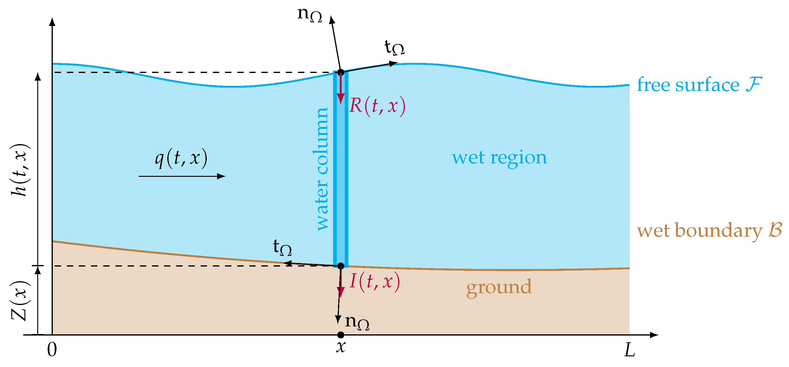
With numerical and practical applications in mind, we assume an arbitrary final time $T>0$. With reference to Figure 1, we consider an incompressible fluid moving in the space–time box

$$\begin{array}{c}[0,T]\times {\mathbb{R}}^2\mathrm{with}\mathrm{typical}\mathrm{point}\mathrm{denoted}(t,x,z)\end{array}.$$

(3)

The absolute height of the surface of the watercourse and the topography of the channel bed are modeled, respectively, by the functions

$$\begin{array}{cccc}\hfill H:& \hfill \left[0,T\right]\times \mathbb{R}& \to & \mathbb{R}\hfill \\ & \hfill (t,x)& \mapsto & H(t,x),\hfill \end{array}\begin{array}{cccc}\hfill Z:& \hfill \mathbb{R}& \to & \mathbb{R}\hfill \\ & \hfill x& \mapsto & Z\left(x\right),\hfill \end{array}$$

(4)

whose values are measured with respect to a reference horizontal height 0. We define the local height of the water by

$$h(t,x):=H(t,x)-Z\left(x\right).$$

(5)

The wet region is defined as the area in which the fluid resides at each time $t\in \left[0,T\right]$

$$\Omega \left(t\right):=\left\{(x,z)\in {\mathbb{R}}^2:Z\left(x\right)<z<H(t,x)\right\},$$

(6)

with its global counterpart

$$\Omega :={\bigcup }_{0\le t\le T}\Omega \left(t\right).$$

(7)

As we can see in Figure 1, the wet region has two boundaries; the first is the wet boundary between the wet region and the ground, denoted by

$$\mathcal{B}=\left\{\right(x,Z):x\in \mathbb{R}\},$$

(8)

and the second is the free surface between the wet region and the surrounding air, denoted by

$$\mathcal{F}=\left\{\right(t,x,H):t>0,x\in \mathbb{R}\}.$$

(9)

We assume that the viscous flow $\mathit{u}$ satisfies, on the space–time domain $\Omega$, the two-dimensional incompressible Navier–Stokes equation

$$\begin{array}{c}\mathrm{div}\left[{\rho }_0\mathit{u}{}^{⊺}\right]=0,\\ {\partial }_t\left[{\rho }_0\mathit{u}\right]+\mathrm{div}\left[{\rho }_0\mathit{u}\otimes \mathit{u}\right]-\mathrm{div}\sigma \left[\mathit{u}\right]-{\rho }_0\mathit{F}=0,\end{array}$$

(10)

where $\mathit{u}=\left(u,\mathit{v}\right)$ is the velocity field, ${\rho }_0$ is the density of the fluid (taken to be constant since the fluid is incompressible), $\mathit{F}=\left(0,-g\right)$ is the external force of gravity with constant g, and $\sigma \left[\mathit{u}\right]$ is the total stress tensor whose matrix is given by

$$\sigma \left[\mathit{u}\right]:=\left[\begin{array}{cc}-p+2\mu {\partial }_{x}u& \mu \left({\partial }_{z}u+{\partial }_x\mathit{v}\right)\\ \mu \left({\partial }_{z}u+{\partial }_x\mathit{v}\right)& -p+2\mu {\partial }_z\mathit{v}\end{array}\right],$$

(11)

where p is the pressure and $\mu >0$ is the dynamic viscosity. The (algebraic) tensor product of two vectors $\mathit{a}\otimes \mathit{b}$ is defined as $\mathit{a}{\mathit{b}}^{⊺}$ (all vectors are displayed as columns), and the $\mathrm{div}$ of a covector/tensor is taken as the row-wise divergence of the associated matrix; in coordinates, this means

$${\left[\mathrm{div}\mathit{\alpha }\right]}_i=\sum _{j=x,z}{\partial }_j{\alpha }_i^j\mathrm{for}i=x,z.$$

(12)

To work with the wet region, we introduce its indicator function

$$\mathsf{\Phi }(t,x,z):={\mathbf{1}}_{\Omega \left(t\right)}(x,z)={\mathbf{1}}_{\left[Z\left(x\right)\le z\le H(t,x)\right]}\mathrm{for}\mathrm{all}t,x,z\in \mathbb{R}.$$

(13)

The function $\mathsf{\Phi }$ is advected by the flow, so its material derivative with respect to the flow $\mathit{u}$ must, therefore, be zero. Moreover, thanks to the incompressibility condition, $\mathsf{\Phi }$ satisfies the following indicator transport equation:

$${\partial }_t\mathsf{\Phi }+{\partial }_x\left[\mathsf{\Phi }u\right]+{\partial }_z\left[\mathsf{\Phi }\mathit{v}\right]=0\mathrm{on}\Omega .$$

(14)

2.2. The Wet Boundary

Crucial to our model derivation is the particular situation on the wet boundary, where the effect of infiltration plays a central role. Given a set $G\in {\mathbb{R}}^2$ and a point $\mathit{x}\in \partial G$, we denote by $t_G\left(\mathit{x}\right)$ the unique normalized tangential vector and by $n_G\left(\mathit{x}\right)$ its outward boundary normal (see Figure 1 for $G=\Omega$).

On the wet boundary, the topography is assumed to be rough, and hence produces friction, which we take into account by considering the following Navier boundary condition:

$$\left(\sigma \left[\mathit{u}\right]n_{\Omega }\right)·t_{\Omega }=-{\rho }_0\left(k\left(\mathit{u}\right)+k_{-}\left(I\right)\right)\mathit{u}·t_{\Omega }\mathrm{on}\mathcal{B}.$$

(15)

We will leave defining $k_{-}\left(I\right)$ for the moment and note that the scalar function $k\left(\mathit{u}\right)$ models a general kinematic friction law on the channel bed:

$$k\left(\xi \right):=(C_{\mathrm{lam}}+C_{\mathrm{tur}}\left|\xi \right|),\mathrm{for}\mathrm{all}\xi \in {\mathbb{R}}^2,$$

(16)

where the friction coefficients $C_{\mathrm{lam}}$ and $C_{\mathrm{tur}}$ (which, by definition, are always non-negative) correspond, respectively, to the laminar and turbulent friction factors [21,22,23,24,25]. The ground may also, due to porosity, absorb water (by infiltration) or inject water (through recharge) from and into the bulk. This mechanism is modeled with the following permeable boundary condition:

$$\mathit{u}(t,x,z)·n_{\Omega }(x,z)=I(t,x)\mathrm{on}\mathcal{B},$$

(17)

where the infiltration function I models the amount of water that leaves ($I>0$) or enters ($I<0$) the flow per elementary boundary element.

The term $k_{-}\left(I\right)$ models the friction effect that occurs when water that is recharging through the ground (at an average microscopic velocity rate of zero) connects with the flow. The magnitude of this effect is given by the parameter $\alpha$, and hence, our infiltration mixing friction law, as anticipated in (2), is given by

$$k_{-}\left(I\right):=\alpha I_{-}=\alpha max(0,-I).$$

(18)

We note that the recharge-induced friction only occurs when water is entering the flow (i.e., $I<0$), and is zero otherwise. Although I should, in principle, be thought of as a function of h, $\mathit{u}$, and possibly their derivatives—particularly $\sigma \left[\mathit{u}\right]$, as in the recognized Beavers–Joseph–Saffman model described, for instance, by Beavers and Joseph [26], Saffman [27], Jäger and Mikelić [28], and Badea et al. [29]—we ignore this in this paper and, for simplicity, consider the function I to be a given piecewise linear function of space–time.

We define $\Omega$’s tangential and outward unit normal vectors on $\mathcal{B}$ by

$$t_{\Omega }(x,Z\left(x\right))=\frac{\left(-1,-{\partial }_{x}Z\left(x\right)\right)}{\sqrt{1+|{\partial }_{x}Z\left(x\right){|}^2}}$$

(19)

and

$$n_{\Omega }(x,Z\left(x\right))=\frac{\left({\partial }_{x}Z\left(x\right),-1\right)}{\sqrt{1+|{\partial }_{x}Z\left(x\right){|}^2}},$$

(20)

respectively, following the convention that the outward normal is the tangential vector rotated by $\pi /2$ counterclockwise. It thus follows that (15) and (17) on $\mathcal{B}$ can be rewritten, respectively, as

$$\begin{array}{c}\begin{array}{c}\hfill \frac{\mu \left({\partial }_{x}v+{\partial }_{z}u\right)\left(1-|{\partial }_{x}Z{|}^2\right)-2\mu \left({\partial }_{x}u-{\partial }_{z}v\right){\partial }_{x}Z}{{\left(1+{|{\partial }_{x}Z|}^2\right)}^{1/2}}\\ \hfill ={\rho }_0\left(k(u,v)+k_{-}\left(I\right)\right)\left(u+v{\partial }_{x}Z\right)\end{array}\end{array}$$

(21)

and

$$\begin{array}{c}\hfill \mathit{v}-u{\partial }_{x}Z\left(x\right)+I\sqrt{1+{|{\partial }_{x}Z|}^2}=0.\end{array}$$

(22)

2.3. The Free Surface

On the free surface, we neglect all other meteorological phenomena (such as evaporation) and consider only the addition of water in the form of direct rainfall and runoff. Assuming a kinematic boundary condition, we set

$$\mathit{u}·n_{\Omega }=\frac{{\partial }_{t}H-R}{\sqrt{1+|{\partial }_{x}H{|}^2}}\mathrm{on}\mathcal{F},$$

(23)

where $R(t,x)$ is the recharge rate due to rainfall. The unit tangential and normal vectors $t_{\Omega }$ and $n_{\Omega }$ to the free surface can be explicitly computed in terms of H as

$$t_{\Omega }(x,H(t,x))=\frac{\left(1,{\partial }_{x}H(t,x)\right)}{\sqrt{1+|{\partial }_{x}H(t,x){|}^2}}$$

(24)

and

$$n_{\Omega }(x,H(t,x))=\frac{\left(-{\partial }_{x}H(t,x),1\right)}{\sqrt{1+|{\partial }_{x}H(t,x){|}^2}},$$

(25)

which leads to the following explicit form of (23):

$${\partial }_{t}H+u{\partial }_{x}H-v=R\mathrm{on}\mathcal{F}.$$

(26)

We also assume a stress condition on the free surface, given by

$$\left(\sigma \left[\mathit{u}\right]n_{\Omega }\right)·t_{\Omega }=-{\rho }_0{k}_{+}\left(R\right)\mathit{u}·t_{\Omega },$$

(27)

where we use the surface mixing friction law

$$k_{+}\left(R\right)=\alpha R,$$

(28)

which takes into account the frictional effect of the additional entering water’s mixing with the flow from various sources (examples include runoff, direct rainfall, and small-scale tributaries), with $\alpha$ again representing the magnitude of this effect (see Section 2.4 for more on mixing friction and references). Using the tangential and normal vectors as above, this condition becomes

$$\frac{\mu \left({\partial }_{x}v+{\partial }_{z}u\right)\left(1-{|{\partial }_{x}H|}^2\right)-2\mu \left({\partial }_{x}u-{\partial }_{z}v\right){\partial }_{x}H}{\sqrt{1+{|{\partial }_{x}H|}^2}}=-{\rho }_0{k}_{+}\left(R\right)\left(u+v{\partial }_{x}H\right).$$

(29)

2.4. Mixing Friction

In adapting the boundary conditions of the Navier–Stokes equations in Section 2.2 and Section 2.3, we included additional terms $k_{+}\left(R\right)$ and $k_{-}\left(I\right)$ that model the friction effect that occurs when water that is falling on the free surface or recharging through the ground, respectively, connects with the flow. The inclusion of these terms avoids certain paradoxical outcomes in the shallow water equation, such as perpetual motion, that otherwise occur when the terms are omitted. Such terms arise naturally from microscopic effects and have been discussed in the hydrology literature, for instance, by Wenzel [16], Yoon and Wenzel [17], Shen and Li [30], Lu et al. [31], where the laws are empirically derived from measurements and account for turbulence.

The rate-to-friction constitutive relations (18) for $k_{-}\left(I\right)$ and (28) for $k_{+}\left(R\right)$, which we take to be piecewise linear with a single slope $\alpha$, could easily be given by more complicated functions that may be nonlinear in I and R and depend also on the nature of the soil or local geometries x, water depth h, and the flow u. The choices for such relations, however, share essential characteristics, such as being monotone functions of I or R, ${\left[k_{-}\right]}_{I=0}={\left[k_{+}\right]}_{R=0}=0$, and possibly homogeneous in the velocity u and the rates of additional water R and I; we consider the simplest such models by taking a linear relation, and defer their refinement to further studies. Furthermore, in this paper, we stick to the simplest case of a single coefficient $\alpha$ for both R and I (or 0 for the latter), leaving the door open to modeling it in future work as two (possibly spatially dependent) separate parameters $x\mapsto {\alpha }_{+}\left(x\right),{\alpha }_{-}\left(x\right)$.

It is worth pointing out that the coefficient $\alpha$ is dimensionless. Indeed, given that the added/subtracted water rate has dimensions $\left[R\right]=\left[I\right]={\mathrm{L}}^2/\mathrm{T}$, the corresponding stress has dimensions

$$\left[{\rho }_0\alpha R\mathit{u}\right]=\left[{\rho }_0\alpha I\mathit{u}\right]=\left[\alpha \right]\mathrm{M}/{\mathrm{L}}^2\times {\mathrm{L}}^2/\mathrm{T}\times \mathrm{L}/\mathrm{T}=\mathrm{ML}/{\mathrm{T}}^2,$$

(30)

while the stress has dimensions $\left[\sigma \left(\mathit{u}\right)n_{\Omega }\right]=\mathrm{ML}/{\mathrm{T}}^2$, whence $\left[\alpha \right]=1$, i.e., dimensionless.

3. Saint-Venant System with Recharge via Vertical Averaging

We now proceed to write the Navier–Stokes equations with adapted boundary conditions in non-dimensional form. Under an assumption on the shallowness of the ratio of the water height to the horizontal domain (represented by a small parameter $\epsilon$), we formally make an asymptotic expansion of the Navier–Stokes system to the hydrostatic approximation at first order. Finally, we derive the Saint-Venant system through an integration on the water height.

This approach follows one established by Gerbeau and Perthame [23], and is also found in Ersoy [32], which differ in the boundary conditions for Navier–Stokes equations. The latter turn into different source terms in Saint-Venant’s equation. Furthermore, we have to take extra care in how we non-dimensionalize our additional precipitation, infiltration, and friction terms. For simplicity, we will start from the two-dimensional Navier–Stokes equations and obtain the one-dimensional Saint-Venant equations, although this procedure can be employed to derive a two-dimensional analogue from the three-dimensional Navier–Stokes, provided the boundary conditions are modified accordingly.

3.1. Dimensionless Navier–Stokes Equations

To derive the Saint-Venant model, we assume that the water height is small with respect to the horizontal length of the domain and that vertical variations in velocity are small compared to the horizontal variations. This is achieved by postulating a small parameter ratio

$$\epsilon :=\frac{D}{L}=\frac{V}{U}\ll 1,$$

(31)

where $D,L,V$, and U are the scales (or units) of, respectively, water height, domain length, vertical fluid velocity, and horizontal fluid velocity. As a consequence, the time scale T is such that

$$T=\frac{L}{U}=\frac{D}{V}.$$

(32)

We also choose the pressure scale to be

$$P:={\rho }_0{U}^2.$$

(33)

The rationale for this choice is that we are focusing on the effect of the horizontal forces as mass per horizontal acceleration, which has a force scale of

$$F:=\left(D{L}^{2-1}{\rho }_0\right)\left(U{T}^{-1}\right),$$

(34)

and these forces are applied to the vertical boundary scale to give the pressure scale

$$F{\left(D{L}^{2-2}\right)}^{-1}=DL{\rho }_{0}U{T}^{-1}{D}^{-1}={\rho }_{0}UL{T}^{-1}={\rho }_0{U}^2.$$

(35)

It is convenient to define the spatial characteristic length, L, and horizontal velocity, U (and, by definition, T), as finite constants with respect to $ϵ\to 0$, while the water height and vertical velocity are defined as $D=ϵL$ and $V=ϵU$, respectively. This allows us to introduce the dimensionless quantities of time $\tilde{t}$, space $(\tilde{x},\tilde{z})$, pressure $\tilde{p}$, and velocity field $(\tilde{u},\tilde{v})$ via the following scaling relations:

$$\begin{array}{cccc}\hfill \tilde{t}& :=\frac{t}{T},\hfill & \hfill \tilde{p}(\tilde{x},\tilde{t},\tilde{z})& :=\frac{p(x,t,z)}{P},\hfill \\ \hfill \tilde{x}& :=\frac{x}{L},\hfill & \hfill \tilde{u}(\tilde{x},\tilde{t},\tilde{z})& :=\frac{u(x,t,z)}{U},\hfill \\ \hfill \tilde{z}& :=\frac{z}{D}=\frac{z}{\epsilon L},\hfill & \hfill \tilde{v}(\tilde{x},\tilde{t},\tilde{z})& :=\frac{v(x,t,z)}{V}=\frac{v(x,t,z)}{\epsilon U}\hfill \end{array}$$

(36)

In the following bind all the “tilde” variables together, i.e., $\tilde{u}$ is a function of $\tilde{t},\tilde{x},\tilde{z}$. Hence, variable-less operators change accordingly, e.g., $\mathrm{div}\tilde{\mathit{u}}$ means $\mathrm{div}{}_{(\tilde{x},\tilde{z})}(\tilde{u},\tilde{v})$ when $\mathrm{div}\mathit{u}$ means $\mathrm{div}{}_{(x,z)}(u,v)$.

We also rescale the laminar and turbulent friction factors as, respectively,

$$C_{\mathrm{lam},0}:=\frac{C_{\mathrm{lam}}}{V}=\frac{C_{\mathrm{lam}}}{ϵU},C_{\mathrm{tur},0}:=\frac{C_{\mathrm{tur}}}{ϵ},$$

(37)

and the infiltration and rainfall rates as, respectively,

$$\begin{array}{c}\hfill \tilde{I}(\tilde{t},\tilde{x}):=\frac{I(t,x)}{V},\tilde{R}(\tilde{t},\tilde{x}):=\frac{R(t,x)}{V}.\end{array}$$

(38)

Note that in the assumed asymptotic setting, $C_{\mathrm{lam},0}$ and $C_{\mathrm{tur},0}$ are constants with respect to $ϵ$, thus implying that $C_{\mathrm{lam}}$ and $C_{\mathrm{tur}}$ vanish linearly with $ϵ\to 0$. Finally, we define the following non-dimensional numbers:

$$\begin{array}{c}\hfill \begin{array}{cccc}\hfill & \mathrm{Froude}’\mathrm{s}\mathrm{number},\hfill & \hfill \mathrm{Fro}& :=U/\sqrt{gD},\hfill \\ \hfill & \mathrm{Reynolds}’\mathrm{s}\mathrm{number}\mathrm{with}\mathrm{respect}\mathrm{to}\mu ,\hfill & \hfill \mathrm{Rey}& :={\rho }_{0}UL/\mu ,\hfill \end{array}\end{array}$$

(39)

and consider the following asymptotic setting

$$\begin{array}{c}\hfill {\mathrm{Rey}}^{-1}=\epsilon {\mu }_0,\end{array}$$

(40)

where ${\mu }_0$ is the viscosity.

Using these dimensionless variables in the Navier–Stokes Equations (10) and (11), and reordering the terms with respect to powers of $\epsilon$, the dimensionless incompressible Navier–Stokes system reads as follows:

$$\begin{array}{cc}\hfill \mathrm{div}\left[\tilde{\mathit{u}}\right]& =0\hfill \\ \hfill {\partial }_{\tilde{t}}\tilde{u}+{\partial }_{\tilde{x}}\left[{\tilde{u}}^2\right]+{\partial }_{\tilde{z}}\left[\tilde{u}\tilde{\mathit{v}}\right]+{\partial }_{\tilde{x}}\tilde{p}& ={\partial }_{\tilde{z}}\left[\frac{{\mu }_0}{\epsilon }{\partial }_{\tilde{z}}\tilde{u}\right]+{\varrho }_{42,\epsilon ,\tilde{\mathit{u}}}\hfill \\ \hfill {\partial }_{\tilde{z}}\tilde{p}& =-\frac{1}{{\mathrm{Fro}}^2}+{\varrho }_{43,\epsilon ,\tilde{\mathit{u}}}\hfill \end{array}$$

(41)

where

$${\varrho }_{42,\epsilon ,\tilde{\mathit{u}}}:=\epsilon {\mu }_0\left(2{\partial }_{\tilde{u}}\tilde{x}\tilde{x}+{\partial }_{\tilde{v}}\tilde{z}\tilde{x}\right)$$

(42)

and

$${\varrho }_{43,\epsilon ,\tilde{\mathit{u}}}:=\epsilon {\mu }_0\left({\partial }_{\tilde{x}\tilde{z}}\tilde{u}+{\epsilon }^2{\partial }_{\tilde{x}\tilde{x}}\tilde{v}+2{\partial }_{\tilde{z}\tilde{z}}\tilde{\mathit{v}}\right)-{\epsilon }^2\left({\partial }_{\tilde{t}}\tilde{\mathit{v}}+{\partial }_{\tilde{x}}\left[\tilde{u}\tilde{\mathit{v}}\right]+{\partial }_{\tilde{z}}\left[{\tilde{\mathit{v}}}^2\right]\right).$$

(43)

Assuming that $\tilde{\mathit{u}}$ has bounded second derivatives, definitions (42) and (43) formally lead to

$${\varrho }_{42,\epsilon ,\tilde{\mathit{u}}}=O\left(\epsilon \right)\mathrm{and}{\varrho }_{43,\epsilon ,\tilde{\mathit{u}}}=O\left(\epsilon \right).$$

(44)

On the wet boundary $\mathcal{B}$, recalling the scaling relations (36) and (38), and noting that

$$\begin{array}{c}\hfill \frac{\partial Z}{\partial x}=\frac{\epsilon L}{L}\frac{\partial \tilde{Z}}{\partial \tilde{x}}=\epsilon {\partial }_{\tilde{x}}\tilde{Z},\end{array}$$

(45)

the dimensionless Navier boundary condition (21) implies

$$\begin{array}{cc}\hfill {\left[\frac{{\partial }_{\tilde{z}}\tilde{u}}{\epsilon \mathrm{Rey}}\right]}_{\mathcal{B}}=& \left(\frac{C_{\mathrm{lam}}}{U}\tilde{u}+C_{\mathrm{tur}}\left(|\tilde{u}|+\epsilon |\tilde{v}|\right)\tilde{u}+\epsilon k_{-}\left(\tilde{I}\right)\tilde{u}\right)\frac{\sqrt{1+{\epsilon }^2{\left({\partial }_{\tilde{x}}\tilde{Z}\right)}^2}}{1-{\epsilon }^2{\left({\partial }_{\tilde{x}}\tilde{Z}\right)}^2}\hfill \\ \hfill & +\underset{O\left({\epsilon }^2\right)}{\underbrace{{\epsilon }^2{\partial }_{\tilde{x}}\tilde{Z}\left(\frac{C_{\mathrm{lam}}}{U}\tilde{v}+C_{\mathrm{tur}}\left(|\tilde{u}|+\epsilon |\tilde{v}|\right)\tilde{v}+\epsilon k_{-}\left(\tilde{I}\right)\tilde{v}\right)\frac{\sqrt{1+{\epsilon }^2{\left({\partial }_{\tilde{x}}\tilde{Z}\right)}^2}}{1-{\epsilon }^2{\left({\partial }_{\tilde{x}}\tilde{Z}\right)}^2}}}\hfill \\ \hfill & -\underset{O\left(\raisebox{1ex}{$\epsilon $}\!\left/ \!\raisebox{-1ex}{$\mathrm{Rey}$}\right.\right)}{\underbrace{\frac{\epsilon }{\mathrm{Rey}}\left({\partial }_{\tilde{x}}\tilde{v}+\frac{2{\partial }_{\tilde{x}}\tilde{Z}\left({\partial }_{\tilde{z}}\tilde{v}-{\partial }_{\tilde{x}}\tilde{u}\right)}{1-{\epsilon }^2{\left({\partial }_{\tilde{x}}\tilde{Z}\right)}^2}\right)}}.\hfill \end{array}$$

(46)

Applying the non-dimensional friction factors (37) and recalling (40), we get

$$\begin{array}{cc}\hfill {\left[\frac{{\partial }_{\tilde{z}}\tilde{u}}{\epsilon \mathrm{Rey}}\right]}_{\mathcal{B}}& =\epsilon \left(C_{\mathrm{lam},\epsilon }\tilde{u}+C_{\mathrm{tur},\epsilon }\left(|\tilde{u}|+\epsilon |\tilde{v}|\right)\tilde{u}+k_{-}\left(\tilde{I}\right)\tilde{u}\right)\frac{\sqrt{1+{\epsilon }^2{\left({\partial }_{\tilde{x}}\tilde{Z}\right)}^2}}{1-{\epsilon }^2{\left({\partial }_{\tilde{x}}\tilde{Z}\right)}^2}+O\left({\epsilon }^2\right)\hfill \\ & =\epsilon \left(C_{\mathrm{lam},\epsilon }\tilde{u}+C_{\mathrm{tur},\epsilon }\left|\tilde{u}\right|\tilde{u}+k_{-}\left(\tilde{I}\right)\tilde{u}\right)+O\left({\epsilon }^2\right)\hfill \\ & =\epsilon \left(k_0\left(\tilde{u}\right)+k_{-}\left(\tilde{I}\right)\right)\tilde{u}+O\left({\epsilon }^2\right),\hfill \end{array}$$

(47)

with asymptotic friction laws

$$\begin{array}{cc}\hfill k_0\left(\xi \right)& :=C_{\mathrm{lam},0}+C_{\mathrm{tur},0}\left|\xi \right|\mathrm{for}\xi \in \mathbb{R}\hfill \\ \hfill k_{-}\left(\tilde{I}\right)& :=\alpha I_{-}=-min(0,\tilde{I})\mathrm{for}\alpha \in \mathbb{R},\hfill \end{array}$$

(48)

on the wet boundary. The permeable boundary condition (22) reads

$$\tilde{v}=\tilde{u}{\partial }_{x}Z-I\sqrt{1+{\epsilon }^2{\left({\partial }_{x}Z\right)}^2}=\tilde{u}{\partial }_{x}Z-I+O\left(\epsilon \right).$$

(49)

For the boundary conditions on the free surface $\mathcal{F}$, applying our non-dimensionalization approach to the kinematic boundary condition (26), we derive

$${\partial }_{\tilde{t}}\tilde{H}+u{\partial }_{\tilde{x}}\tilde{H}-\tilde{v}=\tilde{R},$$

(50)

while we can non-dimensionalize (29) in the same manner as the Navier boundary condition (21) on the wet boundary $\mathcal{B}$, giving

$$\begin{array}{cc}\hfill {\left[\frac{{\partial }_{\tilde{z}}\tilde{u}}{\epsilon \mathrm{Rey}}\right]}_{\mathcal{F}}& =-\epsilon k_{+}\left(\tilde{R}\right)\tilde{u}+O\left({\epsilon }^2\right),\hfill \end{array}$$

(51)

with free surface asymptotic friction law

$$\begin{array}{c}\hfill k_{+}\left(\tilde{R}\right)=\alpha \tilde{R}\mathrm{for}\alpha \in \mathbb{R}.\end{array}$$

(52)

3.2. Remark Slip vs. No-Slip Boundary Condition

The slip-type Navier boundary condition (15), which can prove useful in modeling inundation of dry areas, e.g., may be replaced with a slip boundary condition in the case of river flows. Indeed, the no-slip boundary condition (which may be viewed as a limit case of the Navier boundary condition (15)) is consistent with our derivation (as well as that of Gerbeau and Perthame [23]), and tthe friction constitutive relation (16) plays the role of closure.

3.3. First-Order Approximation of the Dimensionless Navier–Stokes Equations

Dropping all terms of $O\left(\epsilon \right)$ and above in Equations (41)–(51), we deduce the hydrostatic approximation of the dimensionless Navier–Stokes system (cf. [33]):

$$\begin{array}{cc}\hfill {\partial }_x{u}_{\epsilon }+{\partial }_z{v}_{\epsilon }& =0\hfill \end{array}$$

(53)

$$\begin{array}{cc}\hfill {\partial }_t{u}_{\epsilon }+{\partial }_x\left[{u_{\epsilon }}^2\right]+{\partial }_z\left[u_{\epsilon }{v}_{\epsilon }\right]+{\partial }_x{p}_{\epsilon }& ={\partial }_z\left[\frac{{\mu }_0}{\epsilon }{\partial }_z{u}_{\epsilon }\right]\hfill \end{array}$$

(54)

$$\begin{array}{cc}\hfill {\partial }_z{p}_{\epsilon }& =-\frac{1}{{\mathrm{Fro}}^2},\hfill \end{array}$$

(55)

whilst the boundary conditions, as a result of the asymptotic setting (40), simplify to

$$\begin{array}{c}\hfill \left[\frac{{\mu }_0}{\epsilon }{\partial }_z{u}_{\epsilon }\right]=\left(k_0\left(u_{\epsilon }\right)+k_{-}\left(I\right)\right)u_{\epsilon }\mathrm{and}{v}_{\epsilon }=u_{\epsilon }{\partial }_{x}Z-I\mathrm{on}\mathcal{B},\end{array}$$

(56)

and

$$\begin{array}{c}\hfill \left[\frac{{\mu }_0}{\epsilon }{\partial }_z{u}_{\epsilon }\right]=-k_{+}\left(R\right)u_{\epsilon }\mathrm{and}{\partial }_{t}H+u_{\epsilon }{\partial }_{x}H-v_{\epsilon }=R\mathrm{on}\mathcal{F},\end{array}$$

(57)

in view of Equations (47), (49), (51), and (50), respectively. Here, $(u_{\epsilon },v_{\epsilon },p_{\epsilon })$ represents the solution of the first-order dimensionless Navier–Stokes system.

Vertically integrating both members of Equation (55) over $[z,H(t,x\left)\right]$, we obtain the hydrostatic pressure

$$p_{\epsilon }(t,x,H)-p_{\epsilon }(t,x,z)=-\frac{1}{{\mathrm{Fro}}^2}(H(t,x)-z).$$

(58)

Assuming that the pressure exerted by the rain on the free surface $p_{\epsilon }(t,x,H)=p_c$ for some constant $p_c\in \mathbb{R}$ (as we neglected all other meteorological phenomena), this becomes

$$p_{\epsilon }(t,x,z)=\frac{1}{{\mathrm{Fro}}^2}(H(t,x)-z)+p_c.$$

(59)

Moreover, identifying terms at order $\raisebox{1ex}{$1$}\!\left/ \!\raisebox{-1ex}{$\epsilon $}\right.$ in (54), (56), and (57), we obtain the motion by slices decomposition

$$u_{\epsilon }(t,x,z)=u_0(t,x)+O\left(\epsilon \right)$$

(60)

for some function $u_0=u_0(t,x)$, as a consequence of

$$\begin{array}{c}{\partial }_z\left[{\mu }_0{\partial }_z{u}_{\epsilon }\right]=O\left(\epsilon \right),\mathrm{for}z\in (Z\left(x\right),H(t,x))\end{array}$$

(61)

with

$$\begin{array}{c}\hfill {\left[{\mu }_0{\partial }_z{u}_{\epsilon }\right]}_{|z=Z(x)}=O\left(\epsilon \right)\mathrm{and}{\left[{\mu }_0{\partial }_z{u}_{\epsilon }\right]}_{|z=H(t,x)}=O\left(\epsilon \right).\end{array}$$

(62)

Noting $〈u_{\epsilon }(t,x)〉$ as the mean speed of the fluid over the section $\left[Z\right(x),H(t,x\left)\right]$,

$$〈u_{\epsilon }(t,x)〉=\frac{1}{h(t,x)}{\int }_{Z\left(x\right)}^{H(t,x)}{u}_{\epsilon }(t,x,z)dz,$$

(63)

we are able to use the following approximations and drop the first- and higher-order terms in $ϵ$:

$$\begin{array}{c}\hfill u_{\epsilon }(t,x,z)=〈u_{\epsilon }(t,x)〉+O\left(\epsilon \right)\mathrm{and}〈{u_{\epsilon }(t,x)}^2〉={〈u_{\epsilon }(t,x)〉}^2+O\left(\epsilon \right).\end{array}$$

(64)

Although (64) could be taken as an assumption, we obtain it as a consequence of the assumptions of motion by slices (60) and the asymptotic setting (40). As a consequence, the Boussinesq coefficient, also known as Boussinesq $\Gamma$, equals 1. It would be worth discussing whether this comes from reasonable choices of assumptions, but this is not the purpose of this paper, where $\Gamma =1$ suffices. Yang et al. [34] provide an interesting study of the Boussinesq coefficient.

3.4. The Saint-Venant System with Recharge

Keeping (64) in mind and integrating the indicator transport Equation (14) for $z\in \left[Z\right(x),H(t,x\left)\right]$, we get

$$\begin{array}{cc}\hfill 0& ={\int }_{Z\left(x\right)}^{H(t,x)}{\partial }_t\mathsf{\Phi }(t,x,z)+{\partial }_x\left[\mathsf{\Phi }{u}_{\epsilon }\right]+{\partial }_z\left[\mathsf{\Phi }{v}_{\epsilon }\right]dz\hfill \\ & ={\partial }_{t}h+{\partial }_{x}q-{\left[{\partial }_{t}H+u_{\epsilon }{\partial }_{x}H-v_{\epsilon }\right]}_{z=H(t,x)}]+{\left[u_{\epsilon }{\partial }_{x}Z-v_{\epsilon }\right]}_{z=Z\left(x\right)},\hfill \end{array}$$

(65)

where q is the discharge defined by

$$q(t,x):=〈u_{\epsilon }(t,x)〉h(t,x).$$

(66)

In view of the penetration condition (56) and the kinematic boundary condition (57), we deduce the mass-balance equation:

$${\partial }_{t}h+{\partial }_{x}q=S,$$

(67)

where the source term $S:=R-I$ measures the gain or loss of water through the (nonnegative) recharge rate R (ultimately from rainfall) and (signed) infiltration rate, respectively.

Keeping equations (58), (60), and (64) in mind and thanks to the penetration condition (56) and the kinematic boundary condition (57), integrating the left-hand side of (54) for $z\in \left[Z\right(x),H(t,x\left)\right]$, we get

$$\begin{array}{cc}\hfill {\int }_{Z\left(x\right)}^{H(t,x)}\mathrm{LHS}\left(54\right)dz& ={\partial }_{t}q+{\partial }_x\left[\frac{q^2}{h}+\frac{h^2}{2{\mathrm{Fro}}^2}\right]+\frac{h}{{\mathrm{Fro}}^2}{\partial }_{x}Z\hfill \\ & \phantom{=}-{\left[\left({\partial }_{t}H+u_{\epsilon }{\partial }_{x}H-v_{\epsilon }\right)u_{\epsilon }\right]}_{(t,x,H(t,x\left)\right)}\hfill \\ & \phantom{=}+{\left[\left(u_{\epsilon }{\partial }_{x}Z-v_{\epsilon }\right)u_{\epsilon }\right]}_{(t,x,Z(x\left)\right)}\hfill \\ & ={\partial }_{t}q+{\partial }_x\left[\frac{q^2}{h}+\frac{h^2}{2{\mathrm{Fro}}^2}\right]+\frac{h}{{\mathrm{Fro}}^2}{\partial }_{x}Z\hfill \\ & \phantom{=}-R{\left[u_{\epsilon }\right]}_{(t,x,H(t,x\left)\right)}+I{\left[u_{\epsilon }\right]}_{(t,x,Z(x\left)\right)}\hfill \\ & ={\partial }_{t}q+{\partial }_x\left[\frac{q^2}{h}+\frac{h^2}{2{\mathrm{Fro}}^2}\right]+\frac{h}{{\mathrm{Fro}}^2}{\partial }_{x}Z-S\frac{q}{h},\hfill \end{array}$$

(68)

where S is again defined as above. Now, integrating the right-hand side of (54) for $z\in \left[Z\right(x),H(t,x\left)\right]$ using the wet boundary condition (56) and the free surface boundary condition (57), we obtain:

$$\begin{array}{cc}\hfill {\int }_{Z\left(x\right)}^{H(t,x)}\mathrm{RHS}\left(54\right)dz& ={\left[\frac{{\mu }_0}{\epsilon }{\partial }_z{u}_{\epsilon }\right]}_{z=H(t,x)}-{\left[\frac{{\mu }_0}{\epsilon }{\partial }_z{u}_{\epsilon }\right]}_{z=Z\left(x\right)}\hfill \\ & =-\left(k_{+}\left(R\right)+k_{-}\left(I\right)+k_0\left(\frac{q}{h}\right)\right)\frac{q}{h},\hfill \end{array}$$

(69)

where the friction factors $k_{+}\left(R\right)$, $k_{-}\left(I\right)$, and $k_0$ are defined by Formulas (52) and (48), respectively. Finally, multiplying both sides of each of (67)–(69) by ${\rho }_0{U}^2/D$, and recalling the mass-balance (67), we obtain the following Saint-Venant system with recharge:

$$\begin{array}{cc}\hfill {\partial }_{t}h+{\partial }_{x}q& =S:=R-I,\hfill \\ \hfill {\partial }_{t}q+{\partial }_x\left[\frac{q^2}{h}+g\frac{h^2}{2}\right]& =-gh{\partial }_{x}Z+S\frac{q}{h}-\left(k_{+}\left(R\right)+k_{-}\left(I\right)+k_0\left(\frac{q}{h}\right)\right)\frac{q}{h}\hfill \\ \hfill \mathrm{where}q& =hu,\hfill \end{array}$$

(70)

which we study in the rest of this paper.

3.5. Example (Lake at Rest and Filling the Lake)

The still water steady state (also known as lake at rest) reads

$$q\equiv u\equiv S\equiv 0\mathrm{and}h+Z\equiv H_0\mathrm{for}\mathrm{some}\mathrm{constant}{H}_0>0.$$

(71)

This is a classical example used in testing the conservation properties of numerical schemes, based on which we develop some benchmark tests for our schemes. A first interesting nontrivial variation for numerical tests is $S=R-I\equiv 0$ with $R=I\ge 0$. This simple situation has the feature of detecting a scheme that is not well balanced, and is thus considered to be the first benchmark for well-balanced schemes when $R=I=0$.

Another simple (yet important) example is a uniform space–time filling of a lake with initial height $h(0,·)\equiv H_0$ as in (71) with a constant time–space $S>0$ and a spatially constant discharge with periodic boundary conditions. In this case, symmetry implies that system (70) simplifies to

$${\partial }_{t}h\equiv S\mathrm{and}{\partial }_{t}q\equiv S\frac{q}{h}-\left(k_{+}\left(R\right)+k_{-}\left(I\right)+k_0\left(\frac{q}{h}\right)\right)\frac{q}{h},$$

(72)

with given initial conditions.

3.6. Why the Mixing Friction?

To gauge the influence of the friction effect $\alpha$ on the solution, we consider an idealized scenario that will enable us to calculate an exact solution to system (70). We take a constant rainfall–runoff process on a river spanning spatial domain $x\in [0,10]$ and time domain $t\in [0,1]$, with topography $Z\equiv 0.1$; for simplicity, we assume the infiltration $I\equiv 0$ and a linear recharge friction $k_{+}\left(R\right)=\alpha R$. We prescribe periodic boundary conditions and assume a constant initial height and discharge of

$$\begin{array}{c}\hfill h(0,x)=q(0,x)=1\mathrm{for}0<x<10.\end{array}$$

(73)

The rainfall intensity is applied uniformly on the river as a function of time up to the final time $T=1$:

$$\begin{array}{c}\hfill R\left(t\right)=1.0\mathrm{for}0<t<1.\end{array}$$

(74)

Since the rain function, initial height, and initial discharge do not have any dependence on x, we can ignore the spatial derivatives in both the mass (height h) and momentum (discharge q) equations. Under these assumptions, (70) simplifies to:

$${\partial }_{t}h=1,\mathrm{and}{\partial }_{t}q=\left(1-\alpha \right)\frac{q}{h}\mathrm{where}q=hu.$$

(75)

We can solve explicitly for h and q (which are constant in space), as well as the corresponding velocity

$$h(t,x)=t+1,q(t,x)={(t+1)}^{1-\alpha },u(t,x)={(t+1)}^{-\alpha }.$$

(76)

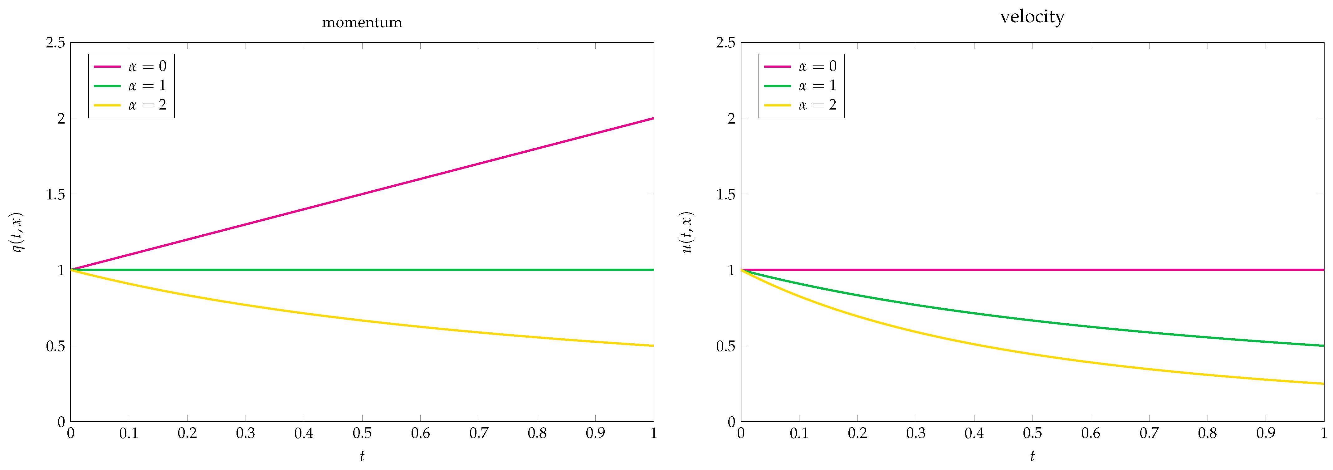
Using these equations, we can plot how the discharge and velocity change over time depending on the mixing friction coefficients $\alpha$. We consider three cases, which are reported in Figure 2. We can conclude from considering this idealized scenario that the additional friction terms cannot be omitted, as doing so leads to a paradoxical situation where the discharge increases over time even though the rain is assumed to be added to the system with zero discharge. We therefore only have physically realistic solutions when the friction $\alpha \ge 1$, as it is within this regime that the discharge is either conserved or decreasing. As is clear from the equations, this occurs when the reduction in velocity is large enough to either compensate or balance the increase in water height.

4. Entropy

Entropy plays an essential role in the analytical and numerical understanding of conservation and balance laws (e.g., [35,36,37,38,39,40]). In this section, we study the effect of the rainfall terms and associated mixing friction on the entropy–entropy-flux pair for the Saint-Venant system (70)—in particular, the effect of the additional rainfall terms on entropy production.

4.1. Theorem (Hyperbolicity and Stability)

Let $(h,q)$ satisfy the Saint-Venant system with recharge (70) for a given topography Z, rainfall R, and infiltration I, with velocity

$$u:=\frac{q}{h}$$

(77)

and total head $\psi :=\widehat{\psi }(h,q,Z)$ defined by

$$\begin{array}{c}\hfill \widehat{\psi }(h,q,Z):=\frac{q^2}{2h^2}+g\left(h+Z\right),for(h,q,Z)\in {\mathbb{R}}^{+}\times {\mathbb{R}}^2.\end{array}$$

(78)

Then, the following hold:

(a)

System (70) is strictly hyperbolic on the set $\left\{h>0\right\}$.

(b)

If $(h,q)$ is smooth and $h>0$, we have the velocity balance equation

$${\partial }_{t}u+{\partial }_x\psi =-\frac{\left(k_{+}\left(R\right)+k_{-}\left(I\right)+k_0\left(u\right)\right)u}{h}.$$

(79)

Proof. 

The proof follows standard arguments from conservation laws and is provided for self-containment’s sake. We consider each statement in turn.

(a)

The Jacobian of (70)’s flux function $(q,h)\mapsto (q,\raisebox{1ex}{$q^2$}\!\left/ \!\raisebox{-1ex}{$h$}\right.+g\raisebox{1ex}{$h^2$}\!\left/ \!\raisebox{-1ex}{$2$}\right.)$ is given by

$$\begin{array}{c}\hfill \mathit{J}=\widehat{\mathit{J}}(h,q):=\left[\begin{array}{cc}0& 1\\ -\raisebox{1ex}{$q^2$}\!\left/ \!\raisebox{-1ex}{$h^2$}\right.+gh& \raisebox{1ex}{$2q$}\!\left/ \!\raisebox{-1ex}{$h$}\right.\end{array}\right],\end{array}$$

(80)

with eigenvalues

$$\begin{array}{c}\hfill {\lambda }_{1,2}={\widehat{\lambda }}_{1,2}(h,q)=\frac{q}{h}\pm \sqrt{gh}.\end{array}$$

(81)

For these eigenvalues to be real and distinct, we require that $h>0$; the Jacobian matrix is thus diagonalizable and system (70) is strictly hyperbolic on the set $\left\{h>0\right\}$.

(b)

We rewrite the conservation of momentum equation in system (70) in terms of the unknowns $(h,u)$, with $u=q/h$, as

$${\partial }_t\left[hu\right]+{\partial }_x\left[h{u}^2+g\frac{h^2}{2}\right]=-gh{\partial }_{x}Z+Su-\left(k_{+}\left(R\right)+k_{-}\left(I\right)+k_0\left(u\right)\right)u.$$

(82)

Applying the product rule to the first term of (82) and substituting in the conservation of mass equation, we get

$$\begin{array}{c}h{\partial }_{t}u+u\left(S-{\partial }_x\left[hu\right]\right)+{\partial }_x\left[h{u}^2\right]+{\partial }_x\left[g\frac{h^2}{2}\right]\hfill \\ \hfill =-gh{\partial }_{x}Z+Su-\left(k_{+}\left(R\right)+k_{-}\left(I\right)+k_0\left(u\right)\right)u,\end{array}$$

(83)

from which we can cancel $Su$ on both sides. Using the product rule again, we have that

$$u{\partial }_x\left[hu\right]={\partial }_x\left[h{u}^2\right]-hu{\partial }_{x}u,$$

(84)

which can be substituted into (83) to give

$$\begin{array}{c}h{\partial }_{t}u-{\partial }_x\left[h{u}^2\right]+hu{\partial }_{x}u+{\partial }_x\left[h{u}^2\right]+{\partial }_x\left[g\frac{h^2}{2}\right]\hfill \\ \hfill =-gh{\partial }_{x}Z-\left(k_{+}\left(R\right)+k_{-}\left(I\right)+k_0\left(u\right)\right)u,\end{array}$$

(85)

enabling us to now cancel ${\partial }_x\left[h{u}^2\right]$. We note that

$${\partial }_x\left[g\frac{h^2}{2}\right]=h{\partial }_x\left[gh\right].$$

(86)

Substituting this into (85) and dividing by h throughout, we get

$${\partial }_{t}u+u{\partial }_{x}u+{\partial }_x\left[gh\right]=-g{\partial }_{x}Z-\frac{\left(k_{+}\left(R\right)+k_{-}\left(I\right)+k_0\left(u\right)\right)u}{h}.$$

(87)

Making the further substitution

$$u{\partial }_{x}u={\partial }_x\left[u^2\right]/2$$

(88)

and grouping derivatives of x, we have

$${\partial }_{t}u+{\partial }_x\psi =-\frac{\left(k_{+}\left(R\right)+k_{-}\left(I\right)+k_0\left(u\right)\right)u}{h}.$$

(89)

The theorem is thus proved. □

4.2. Remark (Friction Effects)

It is worth noting that the only way $S=R-I$ enters in the velocity balance Equation (79) is through the friction terms $k_{+}\left(R\right)$ and $k_{-}\left(I\right)$. This is a further indication that these terms are necessary, especially for small water height h, which, as a denominator of the right-hand side in (79), amplifies the effects of friction, as these occur in the Navier–Stokes on a layer close to the boundaries.

4.3. Theorem (Entropy Production)

Consider the entropy and entropy flux, respectively, defined by

$$\begin{array}{c}\widehat{E}(h,q,Z):=\frac{q^2}{2h}+gh\left(\frac{h}{2}+Z\right)=\frac{h{u}^2+g{h}^2}{2}+ghZ,\end{array}$$

(90)

$$\begin{array}{c}\widehat{\mathsf{\Psi }}(h,q,Z,S):=\left(\widehat{E}(h,q)+\frac{g{h}^2}{2}\right)\frac{q}{h}-g\mathsf{\Theta },\end{array}$$

(91)

where

$$\mathsf{\Theta }(t,x):={\int }_0^{x}S(t,s)Z\left(s\right)dsforeacht>0,x\in \mathbb{R}.$$

(92)

The pair of functions $(\widehat{E},\widehat{\mathsf{\Psi }})$ forms a mathematical entropy–entropy-flux pair for system (70) when $S\equiv 0$ and $k_i=0$ for $i=0,\pm$. Furthermore, for smooth solutions $(h,q)$ of (70), the functions

$$E:=\widehat{E}(h,q,Z)and\mathsf{\Psi }:=\widehat{\mathsf{\Psi }}(h,q,Z,S)$$

(93)

satisfy the following entropy production relation:

$$\begin{array}{c}\hfill {\partial }_{t}E+{\partial }_x\mathsf{\Psi }=S\left(\frac{u^2}{2}+gh\right)-\left(k_{+}\left(R\right)+k_{-}\left(I\right)+k_0\left(u\right)\right)u^2.\end{array}$$

(94)

4.4. Remark (Entropy–Entropy-Flux Pairs and Entropy Production)

The entropy–entropy-flux pair of Theorem 4.3 is typical for shallow water equations (e.g., [18], Th. 2.1). Indeed (94), when $S=0$ and $k_i=0$, for $i=0,\pm$, generalizes the well-known (zero) entropy condition

$${\partial }_{t}E+{\partial }_x\mathsf{\Psi }=0,$$

(95)

which implies that $(\widehat{E},\widehat{\mathsf{\Psi }})$ is an entropy–entropy-flux pair. The additional term $-g\mathsf{\Theta }$ in (91) corresponds to the flux of entropy due to the added or subtracted rain; thanks to this term, the entropy production is frame invariant.

Proof. 

Theorem 4.3: In view of 4.4, it is enough to prove only (94). We begin by recalling that we showed in Theorem 4.1 that the conservation of momentum equation can be rewritten in terms of the velocity u as

$$\begin{array}{c}\hfill {\partial }_{t}u+{\partial }_x\psi =-\frac{\left(k_{+}\left(R\right)+k_{-}\left(I\right)+k_0\left(u\right)\right)u}{h},\end{array}$$

(96)

where $\psi$ is the total head, given by

$$\begin{array}{c}\hfill \psi =\frac{u^2}{2}+gh+gZ.\end{array}$$

(97)

Proceeding from this, multiplying the conservation of mass equation by $\psi$, we have

$$\begin{array}{c}\hfill \psi {\partial }_{t}h+\psi {\partial }_x\left[hu\right]=S\psi ,\end{array}$$

(98)

which we can rewrite as

$$\begin{array}{c}\hfill {\partial }_t\left[\psi h\right]+{\partial }_x\left[\psi hu\right]-\left(h{\partial }_t\psi +\left(hu\right){\partial }_x\psi \right)=S\psi .\end{array}$$

(99)

The term $h{\partial }_t\psi$ in the second component can be expanded as

$$\begin{array}{cc}\hfill h{\partial }_t\psi & =\frac{h}{2}{\partial }_t\left[u^2\right]+hg{\partial }_{t}h+hg{\partial }_{t}Z\hfill \\ & =\left(hu\right){\partial }_{t}u+\frac{g}{2}{\partial }_t\left[h^2\right].\hfill \end{array}$$

(100)

In the second component, we may write

$$\begin{array}{c}\hfill {\partial }_x\psi =-{\partial }_{t}u-\frac{\left(k_{+}\left(R\right)+k_{-}\left(I\right)+k_0\left(u\right)\right)u}{h}\end{array}$$

(101)

from (96), and hence, after cancelling terms, we have

$$\begin{array}{c}\hfill {\partial }_t\left[\psi h\right]+{\partial }_x\left[\psi hu\right]-\left({\partial }_t\left[g\frac{h^2}{2}\right]+\left(k_{+}\left(R\right)+k_{-}\left(I\right)+k_0\left(u\right)\right)u^2\right)=S\psi ,\end{array}$$

(102)

which can be rewritten as

$$\begin{array}{c}\hfill {\partial }_t\left[\psi h-g\frac{h^2}{2}\right]+{\partial }_x\left[\psi hu\right]=S\psi -\left(k_{+}\left(R\right)+k_{-}\left(I\right)+k_0\left(u\right)\right)u^2.\end{array}$$

(103)

Making $\psi$ explicit as a function of $h,q,S,Z$ and noting that

$${\partial }_x\left[g{\int }_0^{x}S(s,t)Z\left(s\right)ds\right]=gS(t,x)Z\left(x\right)\mathrm{for}\mathrm{each}(t,x)$$

(104)

concludes the proof. □

4.5. Remark (Discontinuous Solutions)

In Theorems 4.1 and 4.3, we only made reference to smooth solutions $(h,u)$ in defining the stability and entropy relations of the Saint-Venant system (70). For rough weak solutions, as with conservation laws, the entropy–entropy-flux pair $(\widehat{E},\widehat{\mathsf{\Psi }})$ has the potential to play a selection mechanism role to ensure uniqueness of weak solutions, as it does with conservation laws.

5. The Numerical Model

We now consider the numerical approximation of the Saint-Venant system with rain. We follow the approach developed by Audusse et al. [18], and Perthame and Simeoni [19], with a suitable modification to accommodate the additional source and friction terms. While any well-balanced computational finite volume method could be adapted to simulate our model [36,41,42,43,44,45], the kinetic approach has the pleasant feature of naturally including the additional term $Su$, and thereby also the corresponding friction coefficients $k_{+}\left(R\right)$ and $k_{-}\left(I\right)$, in the Saint-Venant system. As a result, as observed in Audusse et al. [18], the resulting schemes are automatically up-winded and well balanced.

5.1. Well-Balanced Schemes

A desirable property of the standard Saint-Venant system is the preservation of equilibrium states (referred to as the lake at rest), given by

$$\begin{array}{c}\hfill h+Z=constant\mathrm{and}u=0.\end{array}$$

(105)

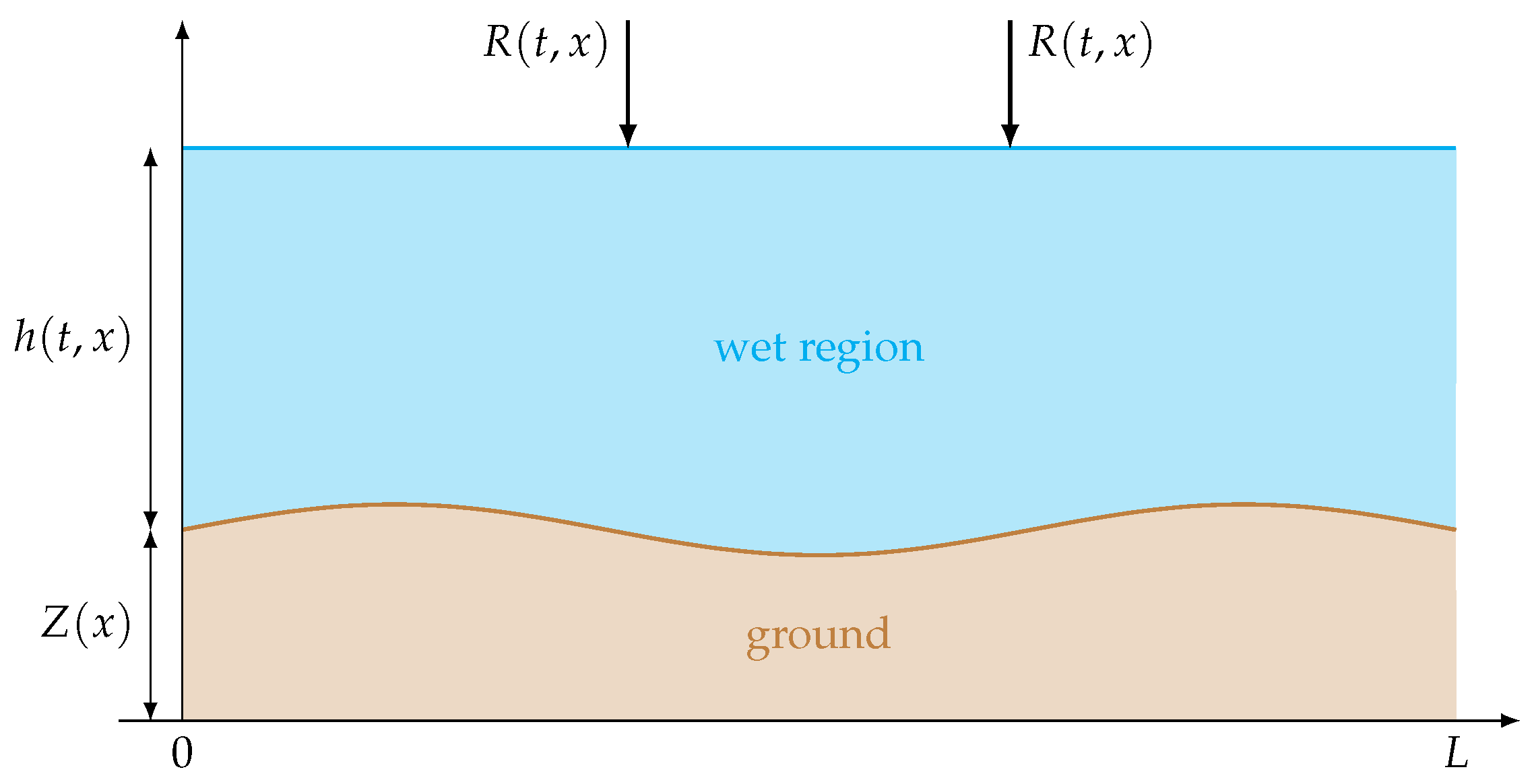
For our system, since, through the addition of rainfall and infiltration effects, we no longer have a conservation law, but rather a balance law, we have the possibility of water being added to or lost from the lake, and thus, this particular equilibrium only holds in the case $S=0$. We must adapt this property, therefore, and instead desire that our system preserves the filling-the-lake state (see Figure 3), given by

$$\begin{array}{c}\hfill {\partial }_{t}h=R\mathrm{and}u=0,\end{array}$$

(106)

that is, the rate at which the water height changes is equal to the rate at which water is added to the system through the rainfall term. Failing to preserve this property would mean that a change is the mass of the water that is greater or lower than the rate at which it is added, thus violating the balance of mass property of our system.

If we wish to maintain this property, we cannot rely on the usual finite difference or finite volume methods, and thus, a new (so-called well-balanced) scheme is required. Such an approach can be found by going back to a kinetic interpretation of the system, as detailed in Perthame and Simeoni [19] and Ersoy [32]. The method we use for the derivation of our kinetic scheme will follow quite the same approach, though with the added complication of accounting for the additional terms. These kinetic solvers can be modified to preserve the filling-the-lake state, while, at the same time, maintaining their simplicity and stability properties.

One of the direct benefits of using such an approach for the Saint-Venant system is the ability of the kinetic solver to deal with dry soil cases (that is, when $h=0$) [18], which will be of importance in ensuring that our model continues to function if infiltration causes the water level to fall close to zero, or if we consider cases such as water flowing away from a beach front.

5.2. Kinetic Function

To derive the kinetic equation for system (70), we follow the kinetic formulation proposed by Audusse et al. [18] and Perthame and Simeoni [19] and further developed by Bourdarias et al. [46] and Ersoy [32]. We consider a kinetic averaging weight function $\chi :\mathbb{R}\to \mathbb{R}$ and a kinetic density function M satisfying

$$\begin{array}{c}\chi \left(\omega \right)=\chi (-\omega )\ge 0,\int \chi \left(\omega \right)d\omega =1,\int {\omega }^2\chi \left(\omega \right)d\omega =\frac{g}{2},\end{array}$$

(107)

$$\begin{array}{c}M(t,x,\xi ):=\sqrt{h(t,x)}\chi \left(\frac{\xi -u(t,x)}{\sqrt{h(t,x)}}\right).\end{array}$$

(108)

These functions originate in the kinetic theory where $M(t,x,\xi )$ accounts for the density of particles with speed $\xi$ at the space–time point $(t,x)$.

In developing a numerical method, the goal is for the derivation of the finite-volume scheme fluxes to be based on M through the following property, which links the macroscopic variables with the microscopic ones.

5.3. Proposition (Macroscopic–Microscopic Relations)

Let the functions $h,u$ solve the Saint-Venant system (70) and M as in (108). If $h(t,x)>0$ at $(t,x)$, then the following macroscopic–microscopic relations hold:

$${\int }_{\mathbb{R}}\left[\begin{array}{c}1\\ \xi \\ {\xi }^2\end{array}\right]M(t,x,\xi )d\xi =\left[\begin{array}{c}h(t,x)\\ h(t,x)u(t,x)\\ h(t,x)u{(t,x)}^2+gh{(t,x)}^2/2\end{array}\right].$$

(109)

5.4. Kinetic Connection to Saint-Venant

Recalling the Saint-Venant system (70), we note that, by substituting $u=\raisebox{1ex}{$q$}\!\left/ \!\raisebox{-1ex}{$h$}\right.$ (for $h>0$), the topography and friction terms on the right-hand side of the conservation of momentum equation can be rewritten as

$$-gh{\partial }_{x}Z-\left(k_{+}\left(R\right)+k_{-}\left(I\right)+k_0\left(u\right)\right)u=-gh\left({\partial }_{x}Z+\frac{\left(k_{+}\left(R\right)+k_{-}\left(I\right)+k_0\left(u\right)\right)u}{gh}\right),$$

(110)

following the approach considered in, for example, Bourdarias et al. [47], adapted to account for our additional friction terms. The reason for rewriting these terms in this manner is so we can pack them into a single divergence form; that is, we define the nonlinear flux integral operator

$$\widehat{W}[h(t,·),u(t,·)]\left(x\right):=Z\left(x\right)+{\int }_0^x\left[\frac{\left(k_{+}\left(R\right)+k_{-}\left(I\right)+k_0\left(u\right)\right)u}{gh}\right](t,s)ds$$

(111)

for each $x\in \mathbb{R}$, and system (70) thus becomes

$$\begin{array}{cc}\hfill {\partial }_{t}h+{\partial }_x\left[hu\right]& =S\hfill \\ \hfill {\partial }_t\left[hu\right]+{\partial }_x\left[h{u}^2+\frac{g{h}^2}{2}\right]& =-gh{\partial }_x\widehat{W}[h,u]+Su.\hfill \end{array}$$

(112)

The kinetic scheme approach allows us to connect the Saint-Venant system with the single scalar equation obtained by introducing an auxiliary microscopic velocity variable $\xi$ and looking at the evolution of the density $\left(0,T\right)\times {\mathbb{R}}^2\ni (t,x,\xi )\mapsto M(t,x,\xi )$ as the solution of the following semilinear kinetic equation:

$${\partial }_{t}M+\xi {\partial }_{x}M-g{\partial }_x\widehat{W}\left[{〈M〉}_0,\frac{{〈M〉}_1}{{〈M〉}_0}\right]{\partial }_{\xi }M+\frac{SM}{{〈M〉}_0}=Q,$$

(113)

where we use the following moment notation for $m=0,1,\dots$:

$${〈M〉}_m:={\int }_{\mathbb{R}}{\xi }^{m}M(·,·,\xi )d\xi .$$

(114)

The right-hand side in (113), $Q(t,x,\xi )$, plays the mathematical role of a collision term, similar, for instance, to the ones encountered in Boltzmann’s equation. In view of Proposition 5.3, if $(h,u)$ satisfying (70) is given, the pair $(M,Q)$ defined by (108) and (113) satisfies the collision 0-moment condition

$${〈Q〉}_m=0\mathrm{for}m=0,1.$$

(115)

Conversely, each pair of functions $(M,Q)$ satisfying (113) and (115) provides a pair $(h,u)$ satisfying (70) by taking

$$h:={〈M〉}_0\mathrm{and}hu:={〈M〉}_1.$$

(116)

5.5. Remark (Advantages of the Kinetic Formulation)

While the kinetic approach is one of many possibilities, and not without drawbacks, we mention some of its nice features:

(i)

In contrast to previous work (e.g., [19]), the kinetic Equation (113) contains an extra term accounting for precipitation and infiltration effects. This departure is crucial for the derivation of the fluxes that lead to a well-balanced scheme in the presence of such terms.

(ii)

We also note that, even though the Maxellian M is constructed for still water steady states, where $S(t,x)=0$, we can still use it here to ensure a well-balanced scheme.

(iii)

In general, it is easier to find a numerical scheme to solve Equation (113) for M that has the properties we desire, such as entropy stability, than to solve the full Saint-Venant system for h and u. However, in finding M, we can calculate h and $hu$ by virtue of the macro-/microscopic relations (Proposition 5.3). In fact, M is never calculated explicitly; rather, the function

$$\begin{array}{c}\widehat{M}(\zeta ,\phi ):=\sqrt{\zeta }\chi \left(\frac{\phi }{\sqrt{\zeta }}\right)\\ \mathrm{where}\mathrm{by}M(t,x,\xi )=\widehat{M}\left(h(t,x),\xi -u(t,x)\right),\end{array}$$

(117)

is used to build the fluxes appearing in a finite volume method, as we shall explain in Section 5.6.

(iv)

As shown and fixed by Xia et al. [48], Buttinger-Kreuzhuber et al. [49], and Taccone et al. [50], some other well-balanced numerical methods fail to correctly represent the effect of the topography, especially when the water height h is close to zero, while the kinetic approach used herein supports arbitrarily small h.

5.6. Discretization and Kinetic Fluxes

To go from the kinetic Equation (113) to a numerical method, we follow the approach of Perthame and Simeoni [19], in which they developed a kinetic scheme for the standard Saint-Venant system, i.e., Equation (113) with $S=0$. Their approach was based on the general method for developing a finite volume scheme, integrating the kinetic equation over the domain of interest, with the vector of unknowns defined as

$$\begin{array}{c}\hfill U_i^n={\int }_{\mathbb{R}}\left[\begin{array}{c}1\\ \xi \end{array}\right]M_i^n\left(\xi \right)d\xi =\left[\begin{array}{c}{h}_i^n\\ h_i^n{u}_i^n\end{array}\right],\end{array}$$

(118)

where the final equality can be seen from the macroscopic–microscopic relations (109) and in view of the second observation above. We follow the same process for our Saint-Venant system, giving us the numerical scheme

$$\begin{array}{c}\hfill U_i^{n+1}=U_i^n-\frac{\Delta t}{\Delta x}\left(F_{i+1/2}^n-F_{i-1/2}^n\right)+\Delta t\left[\begin{array}{c}{S}_i^n\\ S_i^n{u}_i^n\end{array}\right],\end{array}$$

(119)

where $S_i^n$ is a discretization of the combined rain and infiltration terms. We pick the time-step, $\Delta t$, according to

$$\Delta t=\frac{CFL\Delta x}{{max}_i\left(|u_i^n|+\sqrt{2g{h}_i^n}\right)},$$

(120)

where $CFL\in (0,1]$ is the Courant–Friedrichs–Lewy stability constant (e.g., [19]).

The construction of the numerical fluxes $F_{i\pm 1/2}^n$ in (119) is based on the operator associated with $\widehat{M}$ given in (117). We give here a brief overview of how the successive numerical flux terms are developed; the interested reader is directed to Perthame and Simeoni [19] and Bourdarias et al. [46] for more details.

We define the numerical flux (which has two components representing the conservation of mass and momentum equations) as the integral

$$F_{i\pm \frac{1}{2}}^n:={\int }_{\mathbb{R}}\xi \left[\begin{array}{c}1\\ \xi \end{array}\right]M_{i\pm 1/2}^{\mp }\left(\xi \right)d\xi .$$

(121)

The intermediate quantities $M_{i\pm 1/2}^{\mp }\left(\xi \right)$, which measure the flux at the upper and lower boundaries of the cell $c_i=[x_{i-1/2},x_{i+1/2}]$, respectively, are realized as up-winded fluxes:

$$\begin{array}{cc}\hfill M_{i+1/2}^{-}& :=M_i^n\left(\xi \right){\mathbf{1}}_{\left[\xi >0\right]}+M_{i+1/2}^n\left(\xi \right){\mathbf{1}}_{\left[\xi <0\right]},\hfill \\ \hfill M_{i-1/2}^{+}& :=M_i^n\left(\xi \right){\mathbf{1}}_{\left[\xi <0\right]}+M_{i-1/2}^n\left(\xi \right){\mathbf{1}}_{\left[\xi >0\right]},\hfill \end{array}$$

(122)

with

$$\begin{array}{cc}\hfill M_{i\pm 1/2}^n& :=M_i^n(-\xi ){\mathbf{1}}_{\left[{\left|\xi \right|}^2\le 2g\Delta W_{i\pm 1/2}^n\right]}\hfill \\ \hfill & +M_{i\pm 1}^n\left(\mp \sqrt{{\left|\xi \right|}^2-2g\Delta W_{i\pm 1/2}^n}\right){\mathbf{1}}_{\left[{\left|\xi \right|}^2\ge 2g\Delta W_{i\pm 1/2}^n\right]},\hfill \end{array}$$

(123)

where we use the notation

$$\begin{array}{c}\hfill {\mathbf{1}}_{\left[P\right]}:=\left\{\begin{array}{cc}1\hfill & \mathrm{if}P\mathrm{is}\mathrm{true},\hfill \\ 0\hfill & \mathrm{if}P\mathrm{is}\mathrm{false}.\hfill \end{array}\right.\end{array}$$

(124)

To understand how these fluxes are defined, consider the flux over the upper bound $M_{i+1/2}^{-}$. From (122), we can see that it comprises two terms:

(i)

$M_i^n\left(\xi \right){\mathbf{1}}_{\left[\xi >0\right]}$: movement of water with positive velocity ($\xi >0$) from within cell $c_i$ to cell $c_{i+1}$;

(ii)

$M_{i+1/2}^n\left(\xi \right){\mathbf{1}}_{\left[\xi <0\right]}$: movement of water with negative velocity ($\xi <0$) from within cell $c_{i+1}$ to cell $c_i$. This term is decomposed a second time into components reflecting whether the water has enough energy to overcome the topography and friction to enter or leave the cell.

A similar decomposition exists for the second term, $M_{i-1/2}^{+}$, where this time, we consider the negative and positive velocity of $\xi$ for each case, respectively.

The term $\Delta W_{i\pm 1/2}^n$ is the up-winded source term and provides the jump condition necessary for a particle in one cell to overcome the friction and topography to move to an adjacent cell. Consistently with previous definitions, we calculate this term numerically as:

$$\begin{array}{c}\hfill \Delta W_{i+1/2}^n=W_{i+1}\left(t_n\right)-W_i\left(t_n\right),\Delta W_{i-1/2}^n=W_{i-1}\left(t_n\right)-W_i\left(t_n\right),\end{array}$$

(125)

where

$$\begin{array}{c}\hfill W_i\left(t\right)={\mathbf{1}}_{c_i}\left(x\right)\frac{1}{\Delta x}{\int }_{c_i}W(t,x)dx\end{array}$$

(126)

for a given cell $c_i$. The semi-discretized kinetic density, $M_i^n$, is defined as

$$\begin{array}{c}\hfill M_i^n\left(\xi \right):=\sqrt{h_i^n}\chi \left(\frac{\xi -u_i^n}{\sqrt{h_i^n}}\right).\end{array}$$

(127)

The discretization we use in our scheme will be based upon the Barrenblatt kinetic weighting function

$$\chi \left(\omega \right)=\frac{1}{\pi g}\sqrt{{\left(2g-{\omega }^2\right)}_{+}}\mathrm{for}\omega \in \mathbb{R},$$

(128)

where ${\left(X\right)}_{+}$ stands for the positive part of X ([19], Equation (2.13)). We note that this choice of function satisfies the properties we outlined in Section 5.2.

6. Numerical Tests

The kinetic scheme we use for our numerical method was implemented by extending the code of Besson et al. [20] to account for the additional source term in (119), and we present here two simple numerical tests to demonstrate the validity and application of our Saint-Venant system and the associated numerical method. For this paper, we will focus on the rain term only, and thus assume $I\equiv 0$; the coupling of a realistic infiltration model with our Saint-Venant system and the treatment of the boundary conditions would be a paper in itself, and will thus be considered in future research.

In Section 6.1, we compare the accuracy of our numerical model to a flume experiment, considering how our results compare to both the physical data collected from this experiment and also previous numerical simulations of this experiment by other authors. Then, in Section 6.2, we simulate multiple rainfall processes of increasing duration on a slope with both a constant and decreasing gradient, and measure how the value of the friction effect $\alpha$ impacts the solution.

6.1. Comparison with Real-World Data

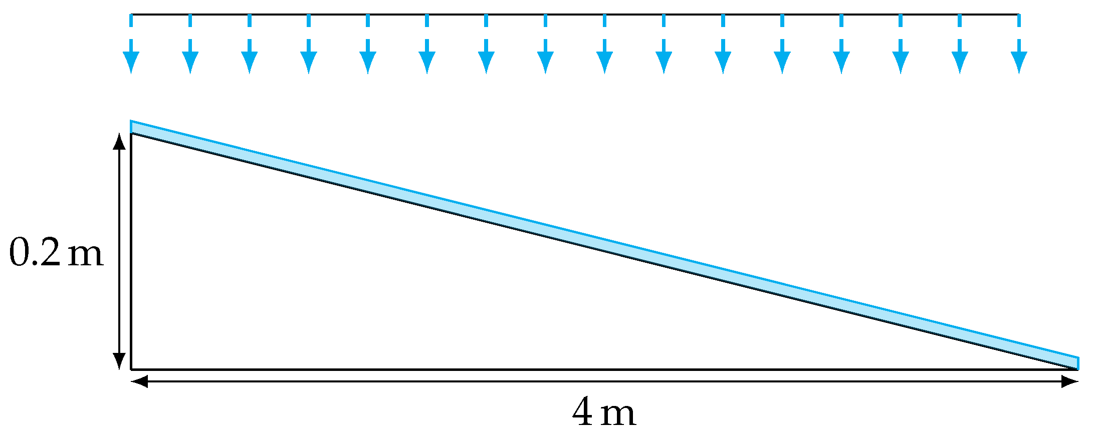
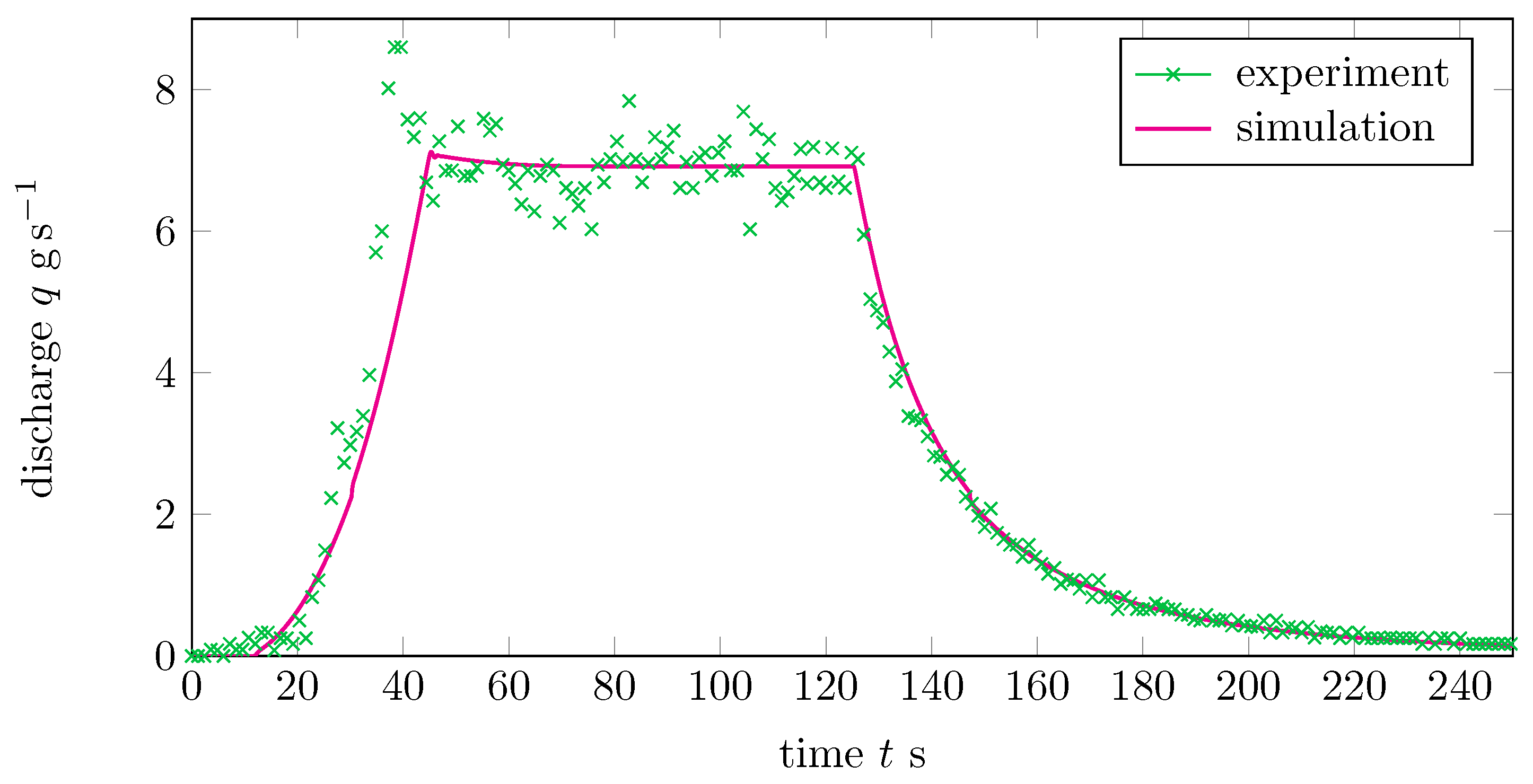
For our first test, we explore the accuracy of our numerical scheme by comparing with data taken from the flume experiment (Figure 4) run as part of the ANR project METHODE at INRA-Orléans; we also compare our results to those obtained by Delestre and James [10], who considered only an addition to the conservation of mass equation.

The experiment in question concerns a slope with a $5\%$ gradient, an initial height $h_0=0$, and initial discharge $q_0=0$. The topography for the slope is given by

$$\begin{array}{cc}\hfill Z\left(x\right)& =0.2-\frac{x}{20}\mathrm{for}x\in [0,4],\hfill \end{array}$$

(129)

we consider $N=1000$ meshpoints, and we assume $CFL=0.95$ (cf. (120)). Rain falls onto the slope uniformly at a constant rate within a given time interval,

$$\begin{array}{c}\hfill R(t,x)=\left\{\begin{array}{cc}50\mathrm{mm}{\mathrm{h}}^{-1}\hfill & \mathrm{if}(t,x)\in [5,125]\times [0,3.95],\hfill \\ 0\hfill & \mathrm{otherwise},\hfill \end{array}\right.\end{array}$$

(130)

and we measure the discharge at the downstream edge of the slope up to time $T=250\mathrm{s}$. For our simulation, we assume the rain-induced friction level $\alpha =1$. The hydrograph for the experiment, together with the simulated values, is provided in Figure 5.

The results from the simulation compare well with the experimental data, particularly in the third and final phase when no rain is falling and the discharge is decreasing gradually over time. For the initial phase, where the discharge is increasing, the simulation matches well to begin with (up to around $25\mathrm{s}$), but subsequently appears to increase at a slower rate than in the experiment; at $t=35\mathrm{s}$, for example, the experiment shows a discharge level of $5.7\mathrm{g}/\mathrm{s}$ compared to the simulation, which is at $3.59\mathrm{g}/\mathrm{s}$. For the secondary phase, where the discharge has stabilized, while the simulation does not capture the fluctuations that were present in the experiment, it does maintain a smooth transition through the center of the data, and begins to decrease at the same point as the experiment.

Comparing the results of our simulation to those of Delestre and James [10], we see that our simulation matches much better in both the initial and final phases; in the initial phase, their simulation increases a lot sooner than in the experiment, and though it begins to decrease at the correct time, it also underestimates the total discharge level in the final phase. For the secondary phase, their results are slightly lower than ours, but are still consistent with the experimental data.

6.2. Single-Level and Three-Level Cascades

For our second test, we consider the classical Iwagaki [51] scenario, which is similar to Section 6.1, but with a higher intensity rainfall–runoff process on a slope with a much shallower gradient. We compare how the water flows when the gradient of the slope is constant and how it flows when the gradient decreases periodically from the upstream to downstream end. We consider a spatial domain $x\in [0,12]$, a final time $t=40\mathrm{s}$, a rainfall intensity $R_0=0.001$ that falls across the entire domain, $N=1000$ meshpoints, and a CFL number of $0.95$. The parameters that we want to change and measure the effect of are the following:

(1)

The total length of the rainfall process $T_R=10\mathrm{s},20\mathrm{s}\mathrm{and}30\mathrm{s}$,

(2)

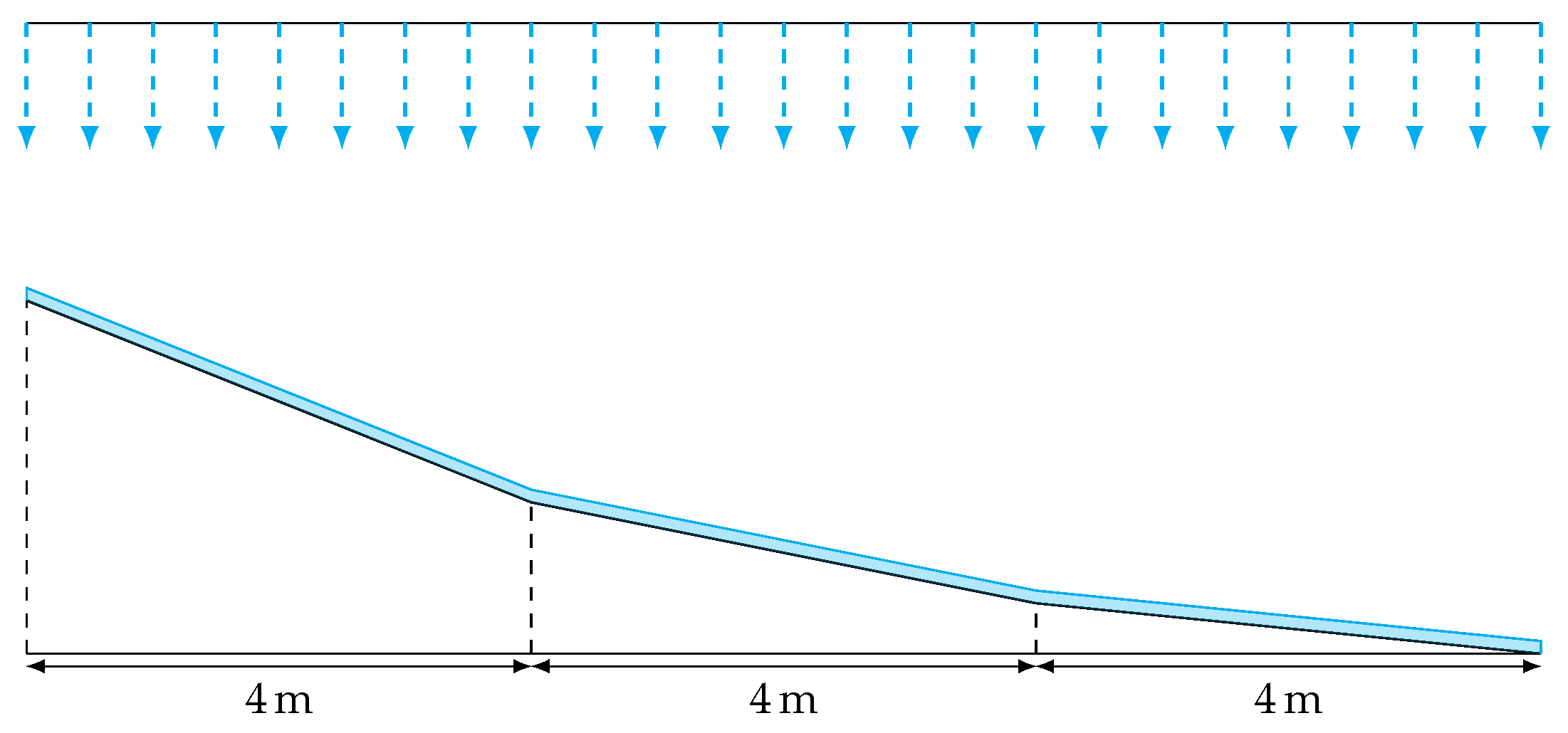
The topography of the slope onto which the rain falls, for which we consider a constant slope (the single cascade) with $Z_1\left(x\right)=(12-x)0.005$ and a decreasing slope (the three-level cascade, see Figure 6) with

$$\begin{array}{cc}\hfill Z_2\left(x\right)& =\left\{\begin{array}{cc}(12-x)0.006-0.012\hfill & \mathrm{if}x\in [0,4]\hfill \\ (12-x)0.005-0.004\hfill & \mathrm{if}x\in [4,8]\hfill \\ (12-x)0.004\hfill & \mathrm{if}x\in [8,12]\hfill \end{array}\right.\hfill \end{array}$$

(131)

(3)

The rain-induced friction level $\alpha$, for which we take $\alpha =0,1,$ and 5 for both the single cascade and the three-level cascade.

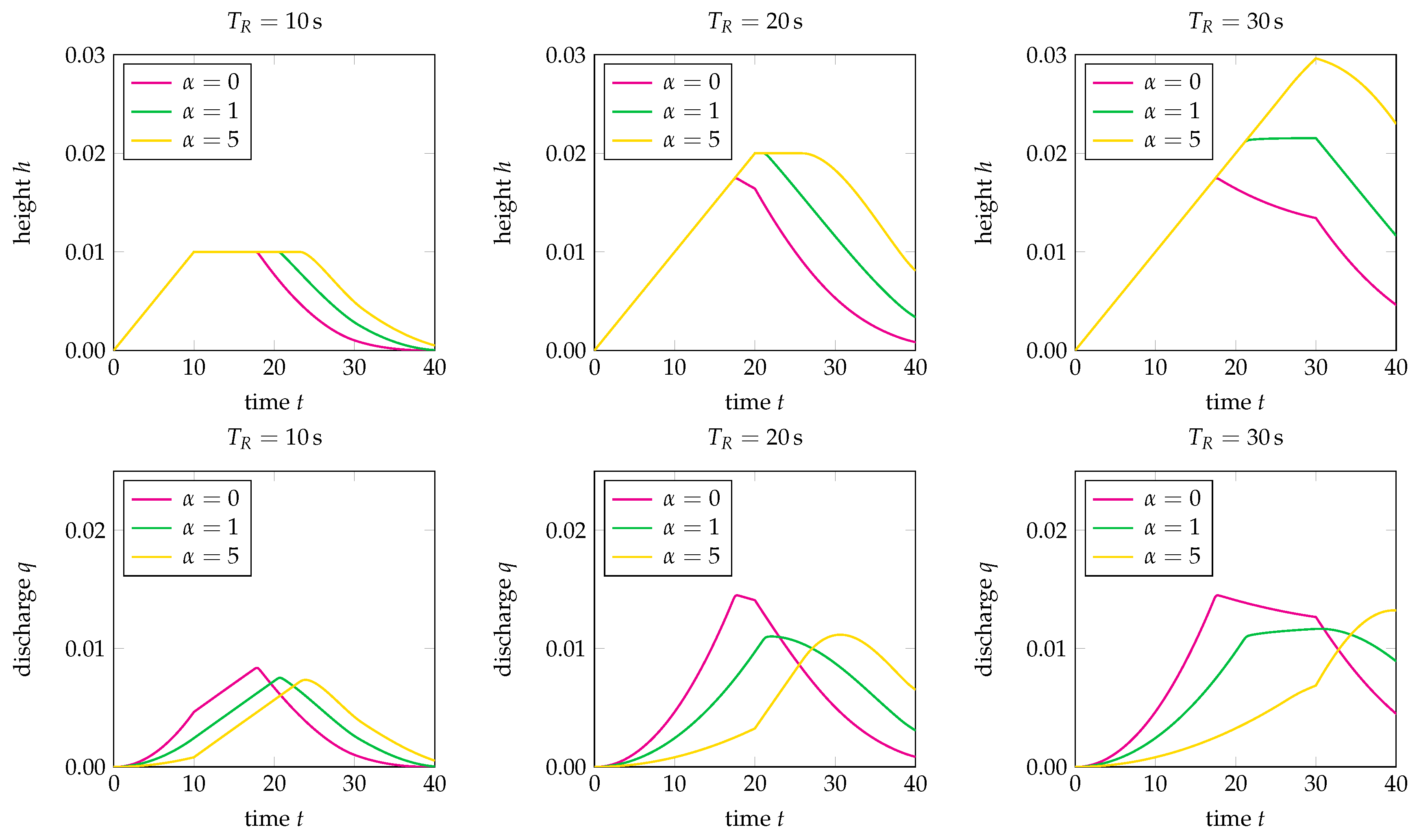
For our outputs, we measure the height of the flow across the entire domain at the point the rainfall stops, and we also measure the height and discharge at the downstream end (i.e., $x=12$) up to the final time.

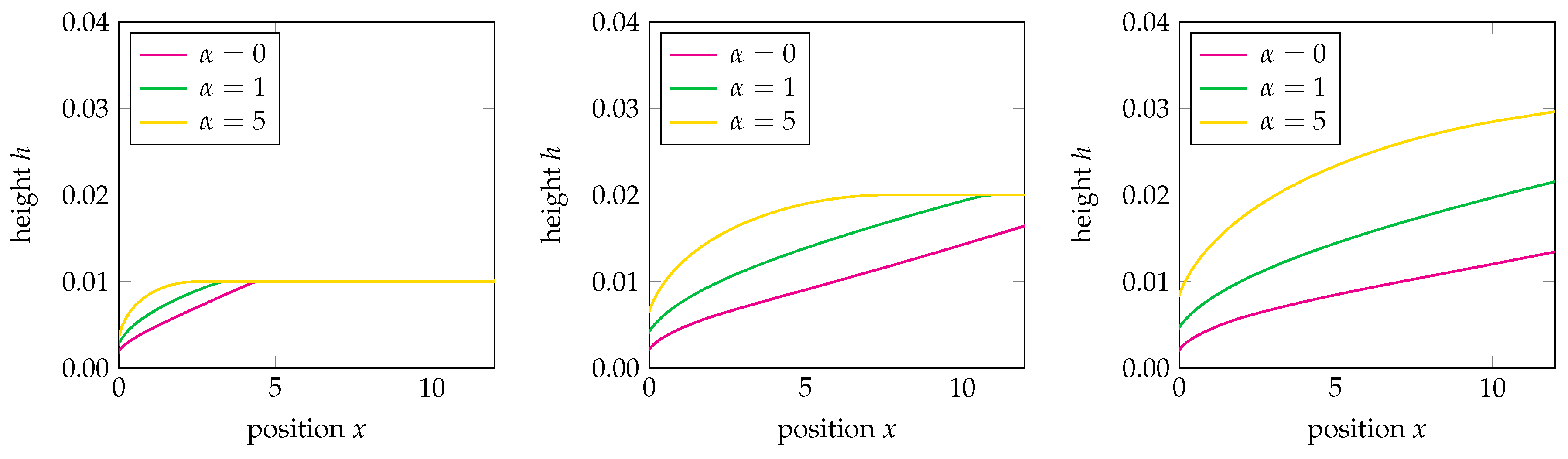
Starting with the height profile at $t=T_R$, we see in Figure 7 that for the single-level cascade, increasing the value of $\alpha$ causes more water to accumulate at the upstream end, as expected, since the discharge of the water will decrease with higher values of $\alpha$. It is interesting to note also that for $T_R=10\mathrm{s}$, the water still accumulates to the same maximum amount irrespective of the value of $\alpha$, though at different points; for longer rainfall times, this accumulation can still occur, but potentially beyond the end of the domain if the water has enough discharge.

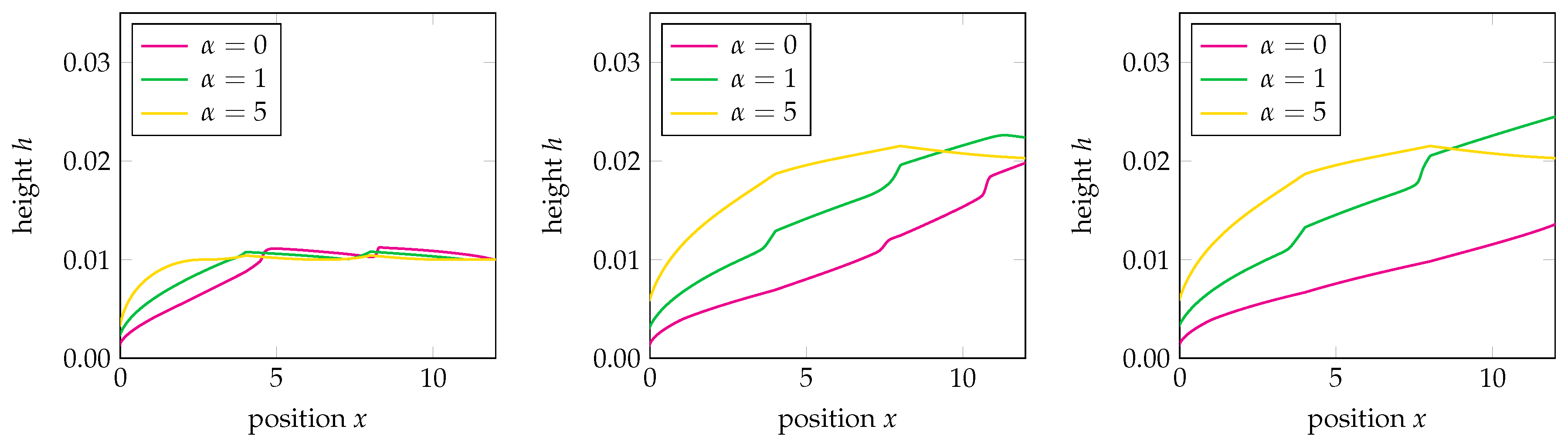
For the three-level cascade shown in Figure 8, the reduction in gradient induces multiple waves to be formed, though these waves become more smoothed out as the rainfall time increases. This effect is reduced as $\alpha$ is increased, consistently with our expectation, since the water flow will be more slowed. The flows do not accumulate to the same amount, though this may be due to the length of the domain.

For the second part of our numerical test, we consider the height and discharge profiles over time at the end of the domain ($x=12\mathrm{m}$). For the single-level cascade (see Figure 9), we see that increasing the friction level $\alpha$ extends the height profile of the flow, causing it to decrease at a later time. This occurs for all lengths of rainfall $T_R$, though notably, we see that as $T_R$ increases, the length of time for which the flow plateaus is decreased.

For the discharge, the change in friction and length of rainfall have a much more pronounced effect. For $T_R=10\mathrm{s}$, the three friction levels result in a profile that shifts as the level increases. For $T_R=20\mathrm{s}\mathrm{and}30\mathrm{s}$, however, the profiles are more varied, with the discharge tending to change rather linearly for $\alpha =0$, but showing a much more curved profile for $\alpha =5$. We can also see that for $T_R=30$, the discharge is decreasing when the rainfall stops for $\alpha =0$ and 1, but continues to rise at an increased rate for $\alpha =5$.

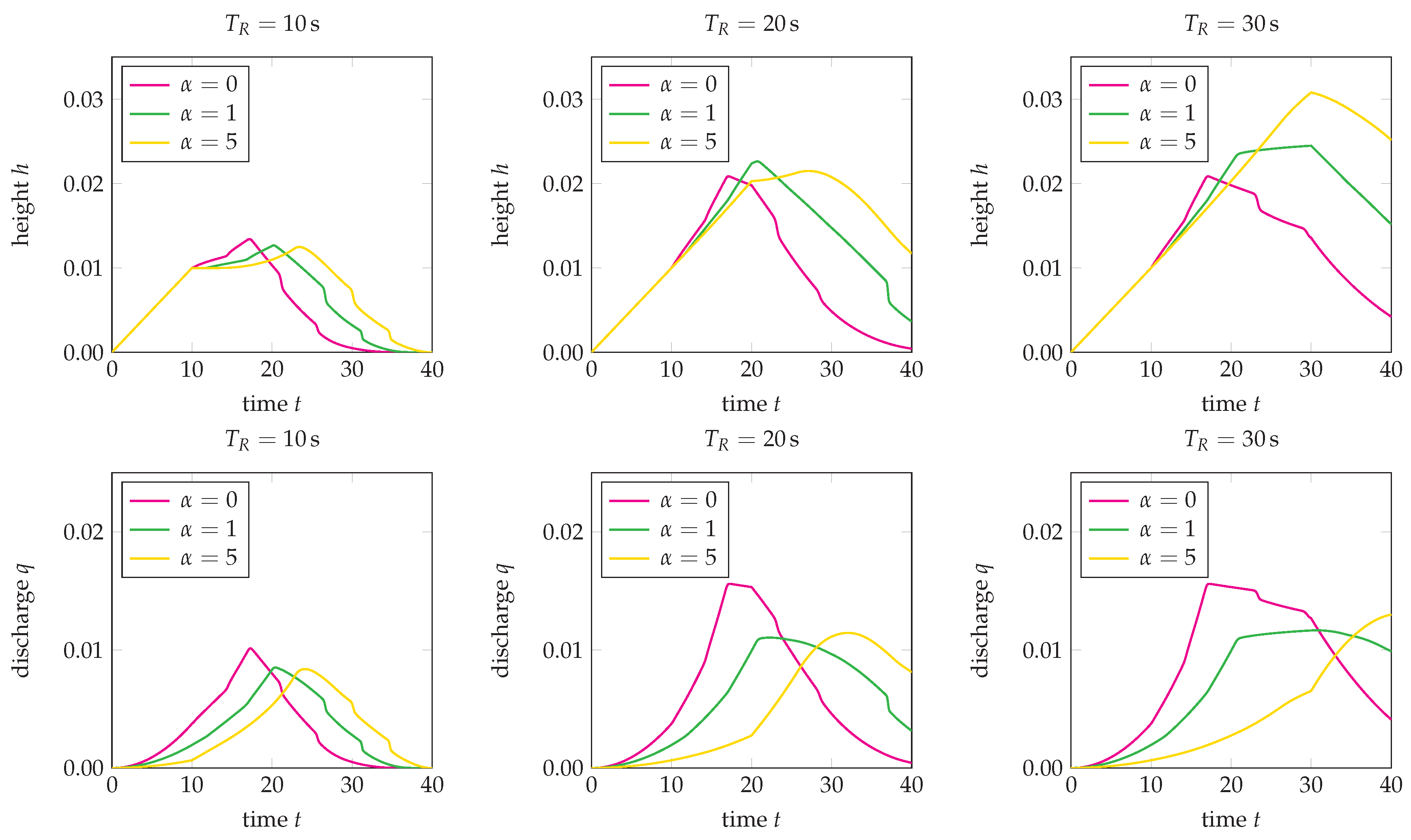
The three-level cascade shown in Figure 10 exhibits a similar behavior to the single-level cascade, with perhaps the most notable changes being in the height profile; for the single-level cascade, the height profile for $\alpha =0$ remains consistently below that for $\alpha =1$, but for the three-level cascade, this does not hold true between, approximately, $t=10$ and $t=20$. The discharge profile for the three-level cascade is very similar in behavior to the single level.

7. Conclusions

Our aim in this paper was a mathematically rigorous derivation of a one-dimensional Saint-Venant system, which was extended to include both precipitation and infiltration effects. Although a special case of this system has been used in the literature, to our knowledge, we present a first derivation from earlier principles. In fact, we went back to the two-dimensional Navier–Stokes equations and adapted the boundary conditions as appropriate to model these additional phenomena (our derivation extends to a $3\mapsto 2$-dimensional case). The new model (70) that we have derived includes additional momentum (discharge) source and friction terms in comparison to other models, which become special cases of our system. The friction terms are obtained naturally from the derivation and their presence is essential in explaining how the velocity of the water body interacts with the additional water coming from either precipitation or runoff; we demonstrated in Section 2.4 that, for certain regimes, this model may yield non-physical solutions. We showed in Theorem 4.1 that the existence of these additional terms leads to a model whose energetic consistency depends solely on the level of assumed rain-induced friction, denoted by $\alpha$.

In developing a numerical model, existing approaches such as finite difference or finite volume can be used, but they fail to ensure certain properties that we would like our method to have. The alternative approach we took was to instead use a kinetic formulation, writing our Saint-Venant system as a single kinetic equation that can then be solved using a finite volume method to find the original variables $(h,q)$. To demonstrate the applicability and viability of our system and the associated kinetic scheme, we ran a number of numerical simulations of our model; in Section 6.1, we compared the accuracy of our model against a real-world experiment, while in Section 6.2, we saw that increasing the value of $\alpha$ slows down the propagation of the flow; these results were all in line with our expectations and analysis of the model.

Though our Saint-Venant model goes some way toward incorporating precipitation and infiltration effects, that it only includes one spatial dimension makes its application to modeling realistic real-world problems limited in scope, particularly on very large domains. The techniques and approach that we have used herein can be readily extended to the two-dimensional system, though some consideration needs to be given to determine the friction terms and kinetic scheme for this system; we note, for example, that it is not clear if the kinetic formulation we have derived for the one-dimensional model can be extended to a second dimension, and thus, an entirely new approach may be required. This work is proposed for future research.

References

- Grace, R.; Eagleson, P.S. Modeling of Overland Flow. Water Resour. Res. 1966, 2, 393–403. [Google Scholar] [CrossRef]
- Woolhiser, D.A.; Liggett, J.A. Unsteady, one-dimensional flow over a plane—The rising hydrograph. Water Resour. Res. 1967, 3, 753–771. [Google Scholar] [CrossRef]
- Zhang, W.; Cundy, T.W. Modeling of two-dimensional overland flow. Water Resour. Res. 1989, 25, 2019–2035. [Google Scholar] [CrossRef]
- Esteves, M.; Faucher, X.; Galle, S.; Vauclin, M. Overland flow and infiltration modelling for small plots during unsteady rain: Numerical results versus observed values. J. Hydrol. 2000, 228, 265–282. [Google Scholar] [CrossRef]
- Weill, S.; Mouche, E.; Patin, J. A generalized Richards equation for surface/subsurface flow modelling. J. Hydrol. 2009, 366, 9–20. [Google Scholar] [CrossRef]
- Rousseau, M.; Cerdan, O.; Ern, A.; Le Maître, O.; Sochala, P. Study of overland flow with uncertain infiltration using stochastic tools. Adv. Water Resour. 2012, 38, 1–12. [Google Scholar] [CrossRef] [Green Version]
- de Saint-Venant, A.J.C.B. Théorie du mouvement non-permanent des eaux, avec application aux crues des rivières at à l’introduction des marées dans leur lit. C. R. Hebd. SéAnces L’AcadéMie Sci. 1871, 73, 147–154. [Google Scholar]
- Fiedler, F.R.; Ramirez, J.A. A numerical method for simulating discontinuous shallow flow over an infiltrating surface. Int. J. Numer. Methods Fluids 2000, 32, 219–239. [Google Scholar] [CrossRef]
- Sochala, P. Numerical Methods for Subsurface Flows and Coupling with Surface Runoff. Ph.D. Thesis, Ecole des Ponts ParisTech, Champs-sur-Marne, France, 2008. [Google Scholar]
- Delestre, O.; James, F. Simulation of rainfall events and overland flow. In Proceedings of the X International Conference Zaragoza-Pau on Applied Mathematics and Statistics, Jaca, Spain, 15–17 September 2008; Volume 35, pp. 125–135. [Google Scholar]
- Costabile, P.; Costanzo, C.; Macchione, F. Two-dimensional numerical models for overland flow simulations. In River Basin Management V; WIT Press: Southampton, UK, 2009; pp. 137–148. [Google Scholar] [CrossRef] [Green Version]
- Fernández-Pato, J.; Caviedes-Voullième, D.; García-Navarro, P. Rainfall/runoff simulation with 2D full shallow water equations: Sensitivity analysis and calibration of infiltration parameters. J. Hydrol. 2016, 536, 496–513. [Google Scholar] [CrossRef]
- Cea, L.; Bladé, E. A simple and efficient unstructured finite volume scheme for solving the shallow water equations in overland flow applications. Water Resour. Res. 2015, 51, 5464–5486. [Google Scholar] [CrossRef] [Green Version]
- Kirstetter, G.; Hu, J.; Delestre, O.; Darboux, F.; Lagrée, P.Y.; Popinet, S.; Fullana, J.M.; Josserand, C. Modeling rain-driven overland flow: Empirical versus analytical friction terms in the shallow water approximation. J. Hydrol. 2016, 536, 1–9. [Google Scholar] [CrossRef] [Green Version]
- Costabile, P.; Costanzo, C.; Ferraro, D.; Macchione, F.; Petaccia, G. Performances of the New HEC-RAS Version 5 for 2-D Hydrodynamic-Based Rainfall-Runoff Simulations at Basin Scale: Comparison with a State-of-the Art Model. Water 2020, 12, 2326. [Google Scholar] [CrossRef]
- Wenzel, H.G.J. The Effect of Raindrop Impact and Surface Roughness on Sheet Flow; Research Report 34; FINAL REPORT Project No. B-018-ILL; Water Rresearch Centre University of Illinois: Urbana-Champaign, IL, USA, 1970. [Google Scholar]
- Yoon, Y.N.; Wenzel, H.G. Mechanics of sheet flow under simulated rainfall. J. Hydraul. Div. 1971, 97, 1367–1386. [Google Scholar]
- Audusse, E.; Bristeau, M.O.; Perthame, B. Kinetic Schemes for Saint-Venant Equations with Source Terms on Unstructured Grids; Research Report RR-3989; Projet M3N; INRIA: Le Chesnay-Rocquencourt, French, 2000. [Google Scholar]
- Perthame, B.; Simeoni, C. A kinetic scheme for the Saint-Venant system with a source term. Calcolo 2001, 38, 201–231. [Google Scholar] [CrossRef]
- Besson, M.; Lakkis, O.; Townsend, P. Finite Volume Code 1D Saint Venant. Available online: https://sourceforge.net/projects/finitevolumecode1dsaintvenant/ (accessed on 29 December 2020).
- Wylie, E.B.; Streeter, V.L. Fluid transients; McGraw-Hill International Book Co.: New York, NY, USA, 1978. [Google Scholar]
- Streeter, V.L.; Wylie, E.B.; Bedford, K.W. Fluid Mech.; OCLC: 37475163; WCB/McGraw Hill: Boston, MA, USA, 1998. [Google Scholar]
- Gerbeau, J.F.; Perthame, B. Derivation of viscous Saint-Venant system for laminar shallow water; numerical validation. Discret. Contin. Dyn. Syst. Ser. B 2001, 1, 89–102. [Google Scholar] [CrossRef]
- Levermore, C.D.; Sammartino, M. A shallow water model with eddy viscosity for basins with varying bottom topography. Nonlinearity 2001, 14, 1493. [Google Scholar] [CrossRef]
- Marche, F. Derivation of a new two-dimensional viscous shallow water model with varying topography, bottom friction and capillary effects. Eur. J. Mech. B Fluids 2007, 26, 49–63. [Google Scholar] [CrossRef]
- Beavers, G.S.; Joseph, D.D. Boundary conditions at a naturally permeable wall. J. Fluid Mech. 1967, 30, 197–207. [Google Scholar] [CrossRef]
- Saffman, P.G. On the Boundary Condition at the Surface of a Porous Medium. Stud. Appl. Math. 1971, 50, 93–101. [Google Scholar] [CrossRef]
- Jäger, W.; Mikelić, A. On the interface boundary condition of Beavers, Joseph, and Saffman. SIAM J. Appl. Math. 2000, 60, 1111–1127. [Google Scholar] [CrossRef]
- Badea, L.; Discacciati, M.; Quarteroni, A. Numerical analysis of the Navier–Stokes/Darcy coupling. Numer. Math. 2010, 115, 195–227. [Google Scholar] [CrossRef] [Green Version]
- Shen, H.W.; Li, R. Rainfall effect on sheet flow over smooth surface. J. Hydraul. Div. 1973, 99, 771–792. [Google Scholar]
- Lu, J.Y.; Chen, J.Y.; Chang, F.H.; Lu, T.F. Characteristics of Shallow Rain-Impacted Flow over Smooth Bed. J. Hydraul. Eng. 1998, 124, 1242–1252. [Google Scholar] [CrossRef]
- Ersoy, M. Dimension reduction for incompressible pipe and open channel flow including friction. In Proceedings of the International Conference Applications of Mathematics 2015, in Honor of the Birthday Anniversaries of Ivo Babuška (90) and Milan Práger (85) and Emil Vitásek(85); Brandts, J., Korotov, S., Křížek, M., Segeth, K., Šístek, J., Vejchodský, T., Eds.; Czech Academy of Sciences: Staré Město, Czech Republic, 2015; pp. 17–33. [Google Scholar]
- De Vita, F.; Lagrée, P.Y.; Chibbaro, S.; Popinet, S. Beyond Shallow Water: Appraisal of a numerical approach to hydraulic jumps based upon the Boundary Layer theory. Eur. J. Mech. B Fluids 2020, 79, 233–246. [Google Scholar] [CrossRef]
- Yang, F.; Liang, D.; Xiao, Y. Influence of Boussinesq coefficient on depth-averaged modelling of rapid flows. J. Hydrol. 2018, 559, 909–919. [Google Scholar] [CrossRef]
- Serre, D. Systems of Conservation Laws 1: Hyperbolicity, Entropies, Shock Waves; Cambridge University Press: Cambridge, UK, 1999. [Google Scholar]
- Bouchut, F. Nonlinear Stability of Finite Volume Methods for Hyperbolic Conservation Laws: And Well-Balanced Schemes for Sources; Frontiers in Mathematics, Birkhäuser Basel: Basel, Switzerland, 2004. [Google Scholar]
- Dafermos, C.M. Hyperbolic Conservation Laws in Continuum Physics, 3rd ed.; Grundlehren der Mathematischen Wissenschaften [Fundamental Principles of Mathematical Sciences]; Springer: Berlin/Heidelberg, Germany, 2010; Volume 325, p. xxxvi+708. [Google Scholar]
- Bouchut, F.; Morales de Luna, T. A subsonic-well-balanced reconstruction scheme for shallow water flows. SIAM J. Numer. Anal. 2010, 48, 1733–1758. [Google Scholar] [CrossRef] [Green Version]
- Evans, L.C. Entropy and Partial Differential Equations; Online Lecture Notes; Department of Mathematics, UC Berkeley: Berkeley, CA, USA, 2013. [Google Scholar]
- Bouchut, F.; Lhébrard, X. A multi well-balanced scheme for the shallow water MHD system with topography. Numer. Math. 2017, 136, 875–905. [Google Scholar] [CrossRef] [Green Version]
- Kröner, D. Numerical Schemes for Conservation Laws; Chichester, B., Teubner Stuttgart, G., Eds.; Wiley-Teubner Series Advances in Numerical Mathematics; John Wiley & Sons, Ltd.: Hoboken, NJ, USA, 1997; p. viii+508. [Google Scholar]
- LeVeque, R.J. Numerical Methods for Conservation Laws, 2nd ed.; Lectures in Mathematics ETH Zürich, Birkhäuser Verlag: Basel, Switerland, 1992; p. x+214. [Google Scholar] [CrossRef]
- LeVeque, R.J. Finite Volume Methods for Hyperbolic Problems; Cambridge Texts in Applied Mathematics; Cambridge University Press: Cambridge, UK, 2002; p. xx+558. [Google Scholar] [CrossRef]
- Toro, E.F. Riemann Solvers and Numerical Methods for Fluid Dynamics, 3rd ed.; A Practical Introduction; Springer: Berlin/Heidelberg, Germany, 2009; p. xxiv+724. [Google Scholar] [CrossRef]
- Kurganov, A. Finite-volume schemes for shallow-water equations. Acta Numer. 2018, 27, 289–351. [Google Scholar] [CrossRef] [Green Version]
- Bourdarias, C.; Ersoy, M.; Gerbi, S. Unsteady mixed flows in non uniform closed water pipes: A full kinetic approach. Numer. Math. 2014, 128, 217–263. [Google Scholar] [CrossRef] [Green Version]
- Bourdarias, C.; Ersoy, M.; Gerbi, S. A kinetic scheme for transient mixed flows in non uniform closed pipes: A global manner to upwind all the source terms. J. Sci. Comput. 2011, 48, 89–104. [Google Scholar] [CrossRef] [Green Version]
- Xia, X.; Liang, Q.; Ming, X.; Hou, J. An efficient and stable hydrodynamic model with novel source term discretization schemes for overland flow and flood simulations. Water Resour. Res. 2017, 53, 3730–3759. [Google Scholar] [CrossRef]
- Buttinger-Kreuzhuber, A.; Horváth, Z.; Noelle, S.; Blöschl, G.; Waser, J. A fast second-order shallow water scheme on two-dimensional structured grids over abrupt topography. Adv. Water Resour. 2019, 127, 89–108. [Google Scholar] [CrossRef]
- Taccone, F.; Antoine, G.; Delestre, O.; Goutal, N. A new criterion for the evaluation of the velocity field for rainfall-runoff modelling using a shallow-water model. Adv. Water Resour. 2020, 140, 103581. [Google Scholar] [CrossRef]
- Iwagaki, Y. Fundamental Studies on the Runoff Analysis by Characteristics; Disaster Prevention Research Institute, Kyoto University: Kyoto, Japan, 1955; Volume 10. [Google Scholar]
- Ambiental. Ambiental Environmental Assessment a Company of Royal HaskoningDHV; Brighton UK and Royal HaskoningDHV: Nijmegen, The Netherlands, 2020; Available online: https://www.ambiental.co.uk/ (accessed on 29 December 2020).
Figure 1.
Diagram of a river and river bed depicting the variables of interest.
Figure 2.
Exact solution’s discharge and velocity in three cases of mixing friction coefficient , as discussed in Section 2.4. The case means no mixing friction whatsoever and leads to a physical paradox where discharge increases in time as mass increases. The case is critical and ensures no artificial discharge gain, but this case is also an unrealistic idealized situation because it implies discharge conservation in the presence of mixing friction. Finally, the case is the most physically relevant.
Figure 3.
In considering a balance law system, we must adapt the lake at rest property used for conservation laws to account for the addition of water.
Figure 4.
Visualization of the flume experiment.
Figure 5.
Hydrograph for the uniform slope test with both the experimental data and the simulated solution.
Figure 6.
Topography for the three-level cascade, showing the decrease in gradient from the upstream to downstream end.
Figure 7.
Height profiles for the single-level cascade for varying values of at the rainfall end time .
Figure 8.
Height profiles for the three-level cascade for values of and 1 at the rainfall end time .
Figure 9.
Height and discharge profiles over time for the single-level cascade for varying values of rain-induced friction at the domain end .
Figure 10.
Height and discharge profiles over time for the three-level cascade for varying values of rain-induced friction at the domain end .
Publisher’s Note: MDPI stays neutral with regard to jurisdictional claims in published maps and institutional affiliations. |
© 2020 by the authors. Licensee MDPI, Basel, Switzerland. This article is an open access article distributed under the terms and conditions of the Creative Commons Attribution (CC BY) license (http://creativecommons.org/licenses/by/4.0/).
Share and Cite
MDPI and ACS Style
Ersoy, M.; Lakkis, O.; Townsend, P. A Saint-Venant Model for Overland Flows with Precipitation and Recharge. Math. Comput. Appl. 2021, 26, 1. https://0-doi-org.brum.beds.ac.uk/10.3390/mca26010001
AMA Style
Ersoy M, Lakkis O, Townsend P. A Saint-Venant Model for Overland Flows with Precipitation and Recharge. Mathematical and Computational Applications. 2021; 26(1):1. https://0-doi-org.brum.beds.ac.uk/10.3390/mca26010001
Chicago/Turabian StyleErsoy, Mehmet, Omar Lakkis, and Philip Townsend. 2021. "A Saint-Venant Model for Overland Flows with Precipitation and Recharge" Mathematical and Computational Applications 26, no. 1: 1. https://0-doi-org.brum.beds.ac.uk/10.3390/mca26010001