Semi-Analytical Solution of Two-Dimensional Viscous Flow through Expanding/Contracting Gaps with Permeable Walls

 ,
,  ,
,  , , ,
, , ,  and
and
Abstract
:1. Introduction
2. Basic Ideas
2.1. Differential Transform Method
2.2. Optimal Homotopy Asymptotic (Analysis) Method
3. Solution
3.1. Differential Transform Method
3.2. Optimal Homotopy Asymptotic Method
3.3. Homotopy Analysis Method
3.4. Adomian Decomposition Method
3.5. Variation Iteration Method
3.6. Reproducing Kernel Hilbert Space Method
3.7. Finite Difference Method for ODEs
3.8. Finite Difference Method for PDE
4. Results and Discussion
5. Conclusions
Author Contributions
Funding
Conflicts of Interest
References
- Nayfeh, A.H. Introduction to Perturbation Technique; Wiley: New York, NY, USA, 1981. [Google Scholar]
- Rand, R.H.; Armbruster, D. Perturbation Methods, Bifurcation Theory and Computer Algebraic; Springer: New York, NY, USA, 1987. [Google Scholar]
- Bouchon, F.; Clain, S.; Touzani, R. A perturbation method for the numerical solution of the Bernoulli problem. J. Comput. Math. 2008, 26, 23–36. [Google Scholar]
- Adomian, G. New approach to nonlinear partial differential equations. J. Math. Anal. Appl. 1984, 102, 420–434. [Google Scholar] [CrossRef] [Green Version]
- Adomian, G. A Review of the Decomposition Method in Applied Mathematics. J. Math. Anal. Appl. 1988, 135, 501–544. [Google Scholar] [CrossRef] [Green Version]
- Adomian, G. Solving Frontier Problems of Physics: The Decomposition Method; Kluwer Academic Publishers: Boston, MA, USA, 1994. [Google Scholar]
- He, J.H. A new approach to non-linear partial differential equations. Commun. Nonlinear Sci. Numer. Simul. 1997, 2, 4. [Google Scholar] [CrossRef]
- He, J.H. Homotopy Perturbation Technique. Comput. Methods Appl. Mech. Eng. 1999, 178, 257–262. [Google Scholar] [CrossRef]
- Zhou, J.K. Differential Transformation and Its Applications for Electrical Circuits; Huazhong University Press: Wuhan, China, 1986. (In Chinese) [Google Scholar]
- Pukhov, G.E. Computational structure for solving differential equations by Taylor transformations. Cybern. Syst. Anal. 1978, 14, 383–390. [Google Scholar] [CrossRef]
- Chen, C.K.; Ho, S.H. Solving partial differential equations by two dimensional differential transform method. Appl. Math. Comput. 1999, 106, 171–179. [Google Scholar]
- Ayaz, F. On the two-dimensional differential transform method. Appl. Math. Comput. 2003, 143, 361–374. [Google Scholar] [CrossRef]
- Ayaz, F. Solutions of the systems of differential equations by differential transform method. Appl. Math. Comput. 2004, 147, 547–567. [Google Scholar] [CrossRef]
- Rashidi, M.M.; Erfani, E. New analytical method for solving Burgers’ and nonlinear heat transfer equations and comparison with HAM. Comput. Phys. Commun. 2009, 180, 1539–1544. [Google Scholar] [CrossRef]
- Rashidi, M.M.; Erfani, E. A Novel Analytical Solution of the Thermal Boundary-Layer over a Flat Plate with a Convective Surface Boundary Condition Using DTM-Padé. Int. Conf. Signal Process. Syst. 2009, 905–909. [Google Scholar]
- Rashidi, M.M.; Basiri Parsab, A.; Anwar Bég, O.; Shamekhi, L.; Sadri, S.M.; Bég, T.A. Parametric analysis of entropy generation in magneto-hemodynamic flow in a semi-porous channel with OHAM and DTM. Appl. Bionics Biomech. 2014, 11, 47–60. [Google Scholar] [CrossRef] [Green Version]
- Liao, S.J. Beyond Perturbation: An Introduction to Homotopy Analysis Method; Chapman Hall/CRC Press: Boca Raton, FL, USA, 2003. [Google Scholar]
- Rashidi, M.M.; Freidoonimehr, N.; Hosseini, A.; Anwar Bég, O.; Hung, T.-K. Homotopy simulation of nanofluid dynamics from a non-linearly stretching isothermal permeable sheet with transpiration. Meccanica 2014, 49, 469–482. [Google Scholar] [CrossRef]
- Marinca, V.; Herisanu, N. Application of optimal homotopy asymptotic method for solving nonlinear equations arising in heat transfer. Int. Commun. Heat Mass Transf. 2008, 35, 710–715. [Google Scholar] [CrossRef]
- Manafian, J.; Sindi, C.T. An optimal homotopy asymptotic method applied to the nonlinear thin film flow problems. Int. J. Numer. Methods Heat Fluid Flow 2018, 28, 2816–2841. [Google Scholar] [CrossRef]
- Khan, M.A.; Ali, N.H.M.; Ullah, S. Application of optimal homotopy asymptotic method for Lane-Emden and Emden-Fowler initial and boundary value problems. AIP Conf. Proc. 2019, 2184, 060022. [Google Scholar]
- Majdalani, J.; Zhou, C.; Dawson, C.A. Two-dimensional viscous flow between slowly expanding or contracting walls with weak permeability. J. Biomech. 2002, 35, 1399–1403. [Google Scholar] [CrossRef]
- Yabushita, K.; Yamashita, M.; Tsuboi, K. An analytic solution of projectile motion with the quadratic resistance law using the homotopy analysis method. J. Phys. A 2007, 40, 8403–8416. [Google Scholar] [CrossRef]
- Cui, M.; Lin, Y. Nonlinear Numerical Analysis in the Reproducing Kernel Space; Nova Science: Hauppauge, NY, USA, 2009. [Google Scholar]
- Wang, Y.; Chaolu, T.; Chen, Z. Using reproducing kernel for solving a class of singular weakly nonlinear boundary value problems. Int. J. Comput. Math. 2010, 87, 367–380. [Google Scholar] [CrossRef]
- Sahihi, H.; Abbasbandy, S.; Allahviranloo, T. Reproducing kernel method for solving singularly perturbed differential-difference equations with boundary layer behavior in Hilbert space. J. Comput. Appl. Math. 2018, 328, 30–43. [Google Scholar] [CrossRef]
- Sahihi, H.; Allahviranloo, T.; Abbasbandy, S. Solving system of second-order BVPs using a new algorithm based on reproducing kernel Hilbert space. Appl. Numer. Math. 2020, 151, 27–39. [Google Scholar] [CrossRef]
- Sahihi, H.; Abbasbandy, S.; Allahviranloo, T. Computational method based on reproducing kernel for solving singularly perturbed differential-difference equations with a delay. Appl. Math. Comput. 2019, 361, 583–598. [Google Scholar] [CrossRef]
- Dinarvand, S.; Rashidi, M.M. A Reliable Treatment of Homotopy Analysis Method for Two-Dimensional Viscous Flow in a Rectangular Domain Bounded by Two Moving Porous Walls. Nonlinear Anal. Real World Appl. 2010, 11, 1502–1512. [Google Scholar] [CrossRef]


| f(y) | Error | ||||||||
|---|---|---|---|---|---|---|---|---|---|
| y | NS | OHAM | DTM | HAM [29] | FDM (21 Nodes) | FDM (41 Nodes) | |NS–OHAM| | |NS–DTM| | |NS–HAM| |
| 0.05 | 0.07968297 | 0.07963688 | 0.08115641 | 0.07976773 | 0.0796722 | 0.0796816 | 0.00004609 | 0.00147343 | 0.00008475 |
| 0.10 | 0.15883439 | 0.15874684 | 0.16174863 | 0.15900660 | 0.158817 | 0.158832 | 0.00008754 | 0.00291423 | 0.00017221 |
| 0.15 | 0.23692796 | 0.23680761 | 0.24121806 | 0.23719225 | 0.236908 | 0.236925 | 0.00012035 | 0.00429009 | 0.00026428 |
| 0.20 | 0.31344783 | 0.31330618 | 0.31901717 | 0.31380922 | 0.313427 | 0.313445 | 0.00014165 | 0.00556933 | 0.00036138 |
| 0.25 | 0.38789339 | 0.38774326 | 0.39461466 | 0.38835539 | 0.387873 | 0.38789 | 0.00015012 | 0.00672126 | 0.00046199 |
| 0.30 | 0.45978377 | 0.45963767 | 0.46750023 | 0.46034624 | 0.459765 | 0.459781 | 0.00014610 | 0.00771645 | 0.00056246 |
| 0.35 | 0.52866181 | 0.52853035 | 0.53718888 | 0.52931903 | 0.528645 | 0.528659 | 0.00013145 | 0.00852706 | 0.00065721 |
| 0.40 | 0.59409750 | 0.59398824 | 0.60322469 | 0.59483670 | 0.594083 | 0.594094 | 0.00010926 | 0.00912718 | 0.00073920 |
| 0.45 | 0.65569090 | 0.65560762 | 0.66518421 | 0.65649164 | 0.655678 | 0.655687 | 0.00008328 | 0.00949330 | 0.00080074 |
| 0.50 | 0.71307445 | 0.71301710 | 0.72267938 | 0.71390897 | 0.713062 | 0.713071 | 0.00005734 | 0.00960493 | 0.00083452 |
| 0.55 | 0.76591479 | 0.76588008 | 0.77536043 | 0.76674949 | 0.765904 | 0.76591 | 0.00003470 | 0.00944564 | 0.00083470 |
| 0.60 | 0.81391411 | 0.81389653 | 0.82291884 | 0.81471214 | 0.813903 | 0.813909 | 0.00001758 | 0.00900472 | 0.00079803 |
| 0.65 | 0.85681100 | 0.85680421 | 0.86509088 | 0.85753578 | 0.8568 | 0.856806 | 0.00000678 | 0.00827988 | 0.00072477 |
| 0.70 | 0.89438098 | 0.89437922 | 0.90166232 | 0.89500031 | 0.89437 | 0.894376 | 0.00000176 | 0.00728134 | 0.00061932 |
| 0.75 | 0.92643663 | 0.92643582 | 0.93247477 | 0.92692704 | 0.926426 | 0.926431 | 0.00000081 | 0.00603813 | 0.00049040 |
| 0.80 | 0.95282750 | 0.95282577 | 0.95743475 | 0.95317819 | 0.952817 | 0.952822 | 0.00000173 | 0.00460724 | 0.00035068 |
| 0.85 | 0.97343970 | 0.97343720 | 0.97652626 | 0.97365547 | 0.97343 | 0.973435 | 0.00000249 | 0.00308655 | 0.00021577 |
| 0.90 | 0.98819530 | 0.98819325 | 0.98982808 | 0.98829784 | 0.988187 | 0.988192 | 0.00000205 | 0.00163278 | 0.00010253 |
| 0.95 | 0.99705157 | 0.99705082 | 0.99753724 | 0.99707830 | 0.997047 | 0.997049 | 0.00000074 | 0.00048567 | 0.00002672 |
| f(y) | Error | ||||||||
|---|---|---|---|---|---|---|---|---|---|
| y | NS | OHAM | DTM | HAM [29] | FDM (21 Nodes) | FDM (41 Nodes) | |NS–OHAM| | |NS–DTM| | |NS–HAM| |
| 0.05 | 0.07968297 | 0.07967858 | 0.07952110 | 0.07966184 | 0.0796722 | 0.0796816 | 0.00000439 | 0.00016186 | 0.00002112 |
| 0.10 | 0.15883439 | 0.15882635 | 0.15851388 | 0.15879237 | 0.158817 | 0.158832 | 0.00000804 | 0.00032051 | 0.00004201 |
| 0.15 | 0.23692796 | 0.23691759 | 0.23645523 | 0.23686548 | 0.236908 | 0.236925 | 0.00001037 | 0.00047273 | 0.00006248 |
| 0.20 | 0.31344783 | 0.31343674 | 0.31283243 | 0.31336535 | 0.313427 | 0.313445 | 0.00001109 | 0.00061540 | 0.00008248 |
| 0.25 | 0.38789339 | 0.38788314 | 0.38714790 | 0.38779137 | 0.387873 | 0.38789 | 0.00001025 | 0.00074549 | 0.00010202 |
| 0.30 | 0.45978377 | 0.45977555 | 0.45892364 | 0.45966263 | 0.459765 | 0.459781 | 0.00000822 | 0.00086008 | 0.00012114 |
| 0.35 | 0.52866181 | 0.52865623 | 0.52770539 | 0.52852210 | 0.528645 | 0.528659 | 0.00000557 | 0.00095642 | 0.00013971 |
| 0.40 | 0.59409750 | 0.59409453 | 0.59306558 | 0.59394019 | 0.594083 | 0.594094 | 0.00000297 | 0.00103192 | 0.00015731 |
| 0.45 | 0.65569090 | 0.65568993 | 0.65460668 | 0.65551782 | 0.655678 | 0.655687 | 0.00000097 | 0.00108421 | 0.00017307 |
| 0.50 | 0.71307445 | 0.71307455 | 0.71196330 | 0.71288878 | 0.713062 | 0.713071 | 0.00000010 | 0.00111114 | 0.00018567 |
| 0.55 | 0.76591479 | 0.76591502 | 0.76480400 | 0.76572147 | 0.765904 | 0.76591 | 0.00000022 | 0.00111079 | 0.00019331 |
| 0.60 | 0.81391411 | 0.81391376 | 0.81283258 | 0.81372003 | 0.813903 | 0.813909 | 0.00000034 | 0.00108152 | 0.00019408 |
| 0.65 | 0.85681100 | 0.85680982 | 0.85578901 | 0.85662477 | 0.8568 | 0.856806 | 0.00000118 | 0.00102199 | 0.00018623 |
| 0.70 | 0.89438098 | 0.89437916 | 0.89344977 | 0.89421221 | 0.89437 | 0.894376 | 0.00000182 | 0.00093121 | 0.00016877 |
| 0.75 | 0.92643663 | 0.92643466 | 0.92562789 | 0.92629467 | 0.926426 | 0.926431 | 0.00000197 | 0.00080874 | 0.00014196 |
| 0.80 | 0.95282750 | 0.95282590 | 0.95217219 | 0.95271967 | 0.952817 | 0.952822 | 0.00000160 | 0.00065531 | 0.00010783 |
| 0.85 | 0.97343970 | 0.97343876 | 0.97296523 | 0.97336934 | 0.97343 | 0.973435 | 0.00000094 | 0.00047446 | 0.00007035 |
| 0.90 | 0.98819530 | 0.98819495 | 0.98791815 | 0.98815995 | 0.988187 | 0.988192 | 0.00000034 | 0.00027715 | 0.00003534 |
| 0.95 | 0.99705157 | 0.99705152 | 0.99695820 | 0.99704187 | 0.997047 | 0.997049 | 0.00000004 | 0.00009336 | 0.00000969 |
| f(y) | Error | ||||||||
|---|---|---|---|---|---|---|---|---|---|
| y | NS | OHAM | DTM | HAM | FDM (21 Nodes) | FDM (41 Nodes) | |NS–OHAM| | |NS–DTM| | |NS–HAM| |
| 0.05 | 0.07968297 | 0.07968261 | 0.07969032 | 0.07967360 | 0.0796722 | 0.0796816 | 0.00000036 | 0.00000734 | 0.00000937 |
| 0.10 | 0.15883439 | 0.15883376 | 0.15884894 | 0.15881583 | 0.158817 | 0.158832 | 0.00000062 | 0.00001455 | 0.00001856 |
| 0.15 | 0.23692796 | 0.23692725 | 0.23694944 | 0.23690053 | 0.236908 | 0.236925 | 0.00000071 | 0.00002147 | 0.00002743 |
| 0.20 | 0.31344783 | 0.31344720 | 0.31347581 | 0.31341189 | 0.313427 | 0.313445 | 0.00000062 | 0.00002797 | 0.00003594 |
| 0.25 | 0.38789339 | 0.38789299 | 0.38792732 | 0.38784923 | 0.387873 | 0.38789 | 0.00000040 | 0.00003392 | 0.00004416 |
| 0.30 | 0.45978377 | 0.45978364 | 0.45982297 | 0.45973162 | 0.459765 | 0.459781 | 0.00000013 | 0.00003919 | 0.00005215 |
| 0.35 | 0.52866181 | 0.52866191 | 0.52870547 | 0.52860185 | 0.528645 | 0.528659 | 0.00000009 | 0.00004366 | 0.00005995 |
| 0.40 | 0.59409750 | 0.59409772 | 0.59414471 | 0.59403005 | 0.594083 | 0.594094 | 0.00000021 | 0.00004720 | 0.00006744 |
| 0.45 | 0.65569090 | 0.65569110 | 0.65574063 | 0.65561664 | 0.655678 | 0.655687 | 0.00000019 | 0.00004973 | 0.00007426 |
| 0.50 | 0.71307445 | 0.71307452 | 0.71312559 | 0.71299468 | 0.713062 | 0.713071 | 0.00000007 | 0.00005114 | 0.00007976 |
| 0.55 | 0.76591479 | 0.76591471 | 0.76596614 | 0.76583167 | 0.765904 | 0.76591 | 0.00000007 | 0.00005135 | 0.00008312 |
| 0.60 | 0.81391411 | 0.81391392 | 0.81396440 | 0.81383072 | 0.813903 | 0.813909 | 0.00000018 | 0.00005028 | 0.00008339 |
| 0.65 | 0.85681100 | 0.85681079 | 0.85685889 | 0.85673122 | 0.8568 | 0.856806 | 0.00000020 | 0.00004789 | 0.00007977 |
| 0.70 | 0.89438098 | 0.89438083 | 0.89442509 | 0.89430910 | 0.89437 | 0.894376 | 0.00000014 | 0.00004411 | 0.00007188 |
| 0.75 | 0.92643663 | 0.92643659 | 0.92647555 | 0.92637671 | 0.926426 | 0.926431 | 0.00000004 | 0.00003891 | 0.00005992 |
| 0.80 | 0.95282750 | 0.95282753 | 0.95285980 | 0.95278254 | 0.952817 | 0.952822 | 0.00000003 | 0.00003229 | 0.00004496 |
| 0.85 | 0.97343970 | 0.97343975 | 0.97346397 | 0.97341082 | 0.97343 | 0.973435 | 0.00000005 | 0.00002426 | 0.00002888 |
| 0.90 | 0.98819530 | 0.98819533 | 0.98821034 | 0.98818107 | 0.988187 | 0.988192 | 0.00000002 | 0.00001504 | 0.00001423 |
| 0.95 | 0.99705157 | 0.99705157 | 0.99705713 | 0.99704775 | 0.997047 | 0.997049 | 0.00000001 | 0.00000556 | 0.00000381 |
| f(y) | Error | ||||||
|---|---|---|---|---|---|---|---|
| y | NS | ADM | VIM | FDM (21 Nodes) | FDM (41 Nodes) | |NS–ADM| | |NS–VIM| |
| 0.05 | 0.07968297 | 0.079683003 | 0.080281204 | 0.0796722 | 0.0796816 | 3.3 × 10⁻⁸ | 0.0005982340 |
| 0.1 | 0.15883439 | 0.15883445 | 0.160014018 | 0.158817 | 0.158832 | 6 × 10⁻⁸ | 0.0011796280 |
| 0.15 | 0.23692796 | 0.236928136 | 0.238655515 | 0.236908 | 0.236925 | 1.76 × 10⁻⁷ | 0.0017275550 |
| 0.2 | 0.31344783 | 0.313448617 | 0.315673608 | 0.313427 | 0.313445 | 7.87 × 10⁻⁷ | 0.0022257780 |
| 0.25 | 0.38789339 | 0.38789674 | 0.390552224 | 0.387873 | 0.38789 | 3.35 × 10⁻⁶ | 0.0026588340 |
| 0.3 | 0.45978377 | 0.45979536 | 0.462796221 | 0.459765 | 0.459781 | 1.159 × 10⁻⁵ | 0.0030124510 |
| 0.35 | 0.52866181 | 0.528695289 | 0.531935936 | 0.528645 | 0.528659 | 3.3479 × 10⁻⁵ | 0.0032741260 |
| 0.4 | 0.59409750 | 0.59418153 | 0.597531318 | 0.594083 | 0.594094 | 8.403 × 10⁻⁵ | 0.0034338180 |
| 0.45 | 0.65569090 | 0.655879857 | 0.659175578 | 0.655678 | 0.655687 | 0.000188957 | 0.0034846780 |
| 0.5 | 0.71307445 | 0.713463776 | 0.716498312 | 0.713062 | 0.713071 | 0.000389326 | 0.0034238620 |
| 0.55 | 0.76591479 | 0.766661934 | 0.769168056 | 0.765904 | 0.76591 | 0.000747144 | 0.0032532660 |
| 0.6 | 0.81391411 | 0.815266027 | 0.816894257 | 0.813903 | 0.813909 | 0.001351917 | 0.0029801470 |
| 0.65 | 0.85681100 | 0.859139281 | 0.859428638 | 0.8568 | 0.856806 | 0.002328281 | 0.0026176380 |
| 0.7 | 0.89438098 | 0.898225607 | 0.896565934 | 0.89437 | 0.894376 | 0.003844627 | 0.0021849540 |
| 0.75 | 0.92643663 | 0.932559563 | 0.928143997 | 0.926426 | 0.926431 | 0.006122933 | 0.0017073670 |
| 0.8 | 0.95282750 | 0.962277299 | 0.954043228 | 0.952817 | 0.952822 | 0.009449799 | 0.0012157280 |
| 0.85 | 0.97343970 | 0.987628762 | 0.974185297 | 0.97343 | 0.973435 | 0.014189062 | 0.0007455970 |
| 0.9 | 0.98819530 | 1.008991505 | 0.988531081 | 0.988187 | 0.988192 | 0.020796205 | 0.0003357810 |
| 0.95 | 0.99705157 | 1.026886619 | 0.997077687 | 0.997047 | 0.997049 | 0.029835049 | 0.0000261170 |
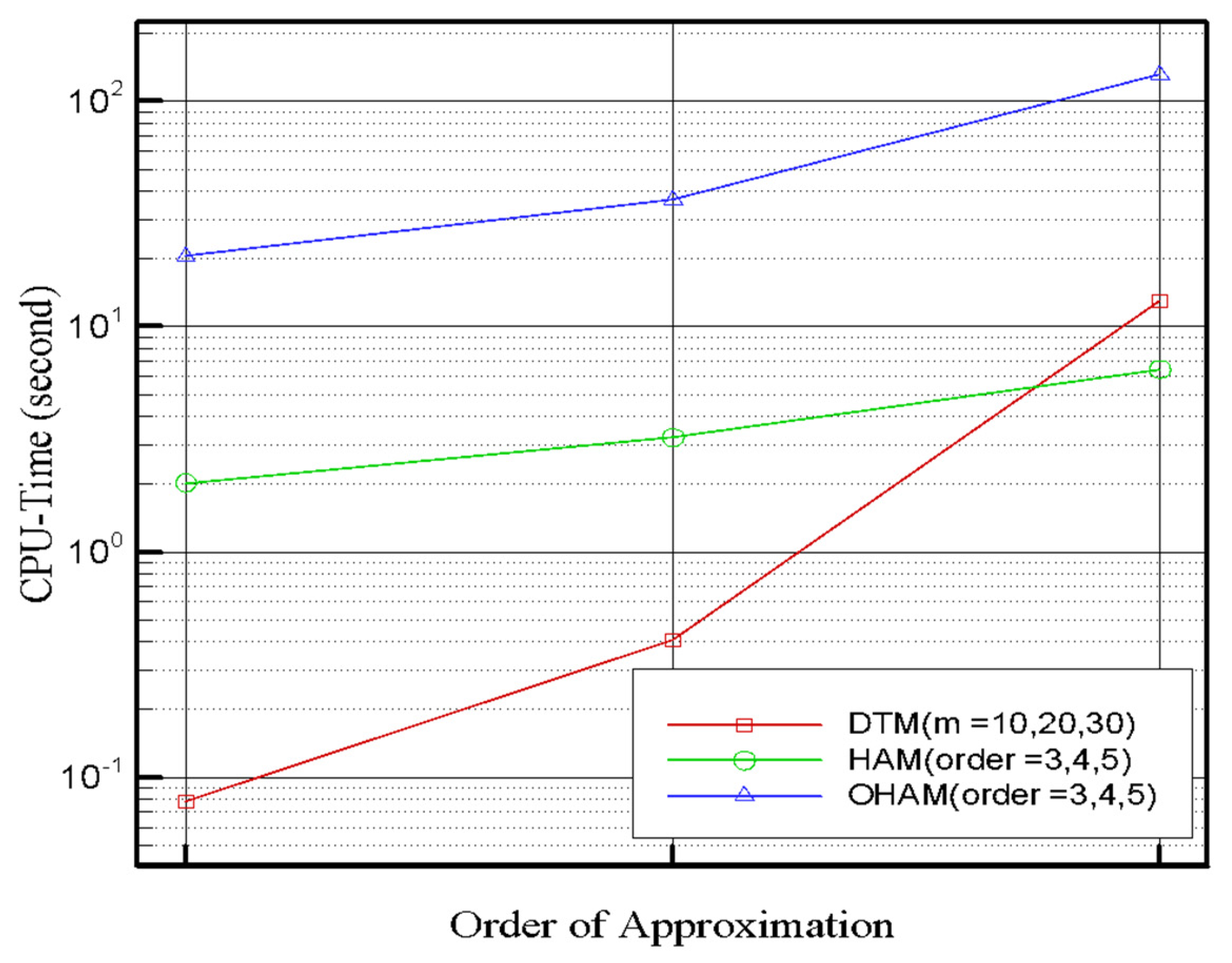
| OHAM | DTM | HAM | |||
|---|---|---|---|---|---|
| Order | CPU-Time | Order | CPU-Time | Order | CPU-Time |
| 3rd-order | 20.547 | m = 10 | 0.078 | 3rd-order | 2.015 |
| 4th-order | 36.515 | m = 20 | 0.406 | 4th-order | 3.219 |
| 5th-order | 131.25 | m = 30 | 13.030 | 5th-order | 6.438 |
| RKHSM | n = 10 | n = 20 | n = 30 | n = 40 | n = 50 | n = 60 | n = 70 |
|---|---|---|---|---|---|---|---|
| Re = 5 | 1.21107 × 10⁻¹¹ | 8.44965 × 10⁻¹² | 6.85690 × 10⁻¹² | 5.91752 × 10⁻¹² | 5.28101 × 10⁻¹² | 4.81348 × 10⁻¹² | 4.45144 × 10⁻¹² |
| Re = 6 | 1.23870 × 10⁻¹⁰ | 8.63987 × 10⁻¹¹ | 7.01099 × 10⁻¹¹ | 6.05043 × 10⁻¹¹ | 5.39960 × 10⁻¹¹ | 4.92156 × 10⁻¹¹ | 4.55138 × 10⁻¹¹ |
| Re = 7 | 7.37340 × 10⁻¹⁰ | 5.14179 × 10⁻¹⁰ | 4.17230 × 10⁻¹⁰ | 3.60064 × 10⁻¹⁰ | 3.21332 × 10⁻¹⁰ | 2.92883 × 10⁻¹⁰ | 2.70854 × 10⁻¹⁰ |
| Re = 8 | 3.05065 × 10⁻⁹ | 2.12697 × 10⁻⁹ | 1.72590 × 10⁻⁹ | 1.48942 × 10⁻⁹ | 1.32920 × 10⁻⁹ | 1.21152 × 10⁻⁹ | 1.12040 × 10⁻⁹ |
| Re = 9 | 9.75283 × 10⁻⁹ | 6.79880 × 10⁻⁹ | 5.51670 × 10⁻⁹ | 4.76080 × 10⁻⁹ | 4.24867 × 10⁻⁹ | 3.87252 × 10⁻⁹ | 3.58124 × 10⁻⁹ |
| Re = 10 | 2.57802 × 10⁻⁸ | 1.79689 × 10⁻⁸ | 1.45803 × 10⁻⁸ | 1.25824 × 10⁻⁸ | 1.12289 × 10⁻⁸ | 1.02348 × 10⁻⁸ | 9.46495 × 10⁻⁹ |
Publisher’s Note: MDPI stays neutral with regard to jurisdictional claims in published maps and institutional affiliations. |
© 2021 by the authors. Licensee MDPI, Basel, Switzerland. This article is an open access article distributed under the terms and conditions of the Creative Commons Attribution (CC BY) license (https://creativecommons.org/licenses/by/4.0/).
Share and Cite
Rashidi, M.M.; Sheremet, M.A.; Sadri, M.; Mishra, S.; Pattnaik, P.K.; Rabiei, F.; Abbasbandy, S.; Sahihi, H.; Erfani, E. Semi-Analytical Solution of Two-Dimensional Viscous Flow through Expanding/Contracting Gaps with Permeable Walls. Math. Comput. Appl. 2021, 26, 41. https://0-doi-org.brum.beds.ac.uk/10.3390/mca26020041
Rashidi MM, Sheremet MA, Sadri M, Mishra S, Pattnaik PK, Rabiei F, Abbasbandy S, Sahihi H, Erfani E. Semi-Analytical Solution of Two-Dimensional Viscous Flow through Expanding/Contracting Gaps with Permeable Walls. Mathematical and Computational Applications. 2021; 26(2):41. https://0-doi-org.brum.beds.ac.uk/10.3390/mca26020041
Chicago/Turabian StyleRashidi, Mohammad Mehdi, Mikhail A. Sheremet, Maryam Sadri, Satyaranjan Mishra, Pradyumna Kumar Pattnaik, Faranak Rabiei, Saeid Abbasbandy, Hussein Sahihi, and Esmaeel Erfani. 2021. "Semi-Analytical Solution of Two-Dimensional Viscous Flow through Expanding/Contracting Gaps with Permeable Walls" Mathematical and Computational Applications 26, no. 2: 41. https://0-doi-org.brum.beds.ac.uk/10.3390/mca26020041