A Straightness Error Compensation System for Topography Measurement Based on Thin Film Interferometry


1
College of Mechanical Engineering and Automation, Huaqiao University, Xiamen 361021, China
2
Advanced Remanufacturing and Technology Centre (Agency for Science, Technology and Research), Singapore 637143, Singapore
3
Institute of Manufacturing Technology, Huaqiao University, Xiamen 361021, China
*
Authors to whom correspondence should be addressed.
Photonics 2021, 8(5), 149; https://0-doi-org.brum.beds.ac.uk/10.3390/photonics8050149
Submission received: 19 April 2021
/
Revised: 27 April 2021
/
Accepted: 28 April 2021
/
Published: 30 April 2021
(This article belongs to the Special Issue Glass Optics)
Abstract
:Straightness error compensation is a critical process for high-accuracy topography measurement. In this paper, a straightness measurement system was presented based on the principle of fringe interferometry. This system consisted of a moving optical flat and a stationary prism placed close to each other. With a properly aligned incident light beam, the air wedge between the optical flat and the prism would generate the interferogram, which was captured by a digital camera. When the optical flat was moving with the motion stage, the variation in air wedge thickness due to the imperfect straightness of the guideway would lead to a phase shift of the interferogram. The phase shift could be calculated, and the air wedge thickness could be measured accordingly using the image processing algorithm developed in-house. This air wedge thickness was directly correlated with the straightness of the motion stage. A commercial confocal sensor was employed as the reference system. Experimental results showed that the repeatability of the proposed film interferometer represented by σ was within 25 nm. The measurement deviation between the film interferometer and the reference confocal sensor was within ±0.1 µm. Compared with other interferometric straightness measurement technologies, the presented methodology was featured by a simplified design and good environment robustness. The presented system could potentially be able to measure straightness in both linear and angular values, and the main focus was to analyze its linear value measurement capability.
1. Introduction
Precision positioning is a key technological enabler for the advanced manufacturing [1,2,3,4] and instrumentation industry [5]. For a precision positioning system, straightness is a very important parameter to assess performance [6]. Especially in the area of topography measurement, the straightness error of the positioners will significantly affect the measurement accuracy [7,8]. How to quantify and compensate the straightness error has become an important research topic in this area [9,10]. In practice, the straightness error can be expressed through linear values (in microns or nanometers) or angular values (in arcseconds or microradians) [11,12,13,14]. Different approaches have been published to quantify the straightness in either way.
There are three types of straightness measurement principles: mechanical-datum-based (Type 1) [15,16], collimated-light-based (Type 2) [17,18], and interferometry-based (Type 3) [19,20,21].
Type 1 is a traditional methodology for measuring linear values in which a displacement probe is usually used to trace the off-axis offsets of a reference line or plane. In Ref. [15], a taut nylon fishing wire was the known reference, and the wire offset was detected by a slotted optical sensor. In Ref. [16], a focused beam formed the displacement probe to trace the reference plane of a reflective wafer surface. The accuracy of this methodology relied on the accuracy of the probe and the quality of the reference line or plane.
Represented by autocollimators, Type 2 is a popular way of quantifying motion errors (mostly angular values) of machine tools and other long-travel systems based on the autocollimation principle and reflection principle. In Ref. [17], a miniature three-degree-of-freedom laser measurement system, including a miniature autocollimator kit, was proposed to measure the straightness of a precision positioning stage. In Ref. [18], a three-axis angular motion error simultaneous detection system composed of two autocollimation units was presented. In this type of system, positioning sensitive detectors (PSDs) were normally used to detect the spot movements, which were correlated with the straightness of the motion stages. Therefore, the accuracy of this methodology was limited by the resolution of the position sensors.
Type 3 based on optical interferometry is suitable for high accuracy measurements. The straightness errors can be obtained from the change in optical path difference. In Ref. [19], a straightness measurement system based on a 2D encoder was proposed. The ±1st order diffracted beams formed the interferogram to measure the displacement correlated with straightness. In Ref. [20], a multi-probe measurement system was equipped with a micro-coordinate measuring machine, in which two laser interferometers were used to separate the angular motion error. In Ref. [21], a six-degree-of-freedom laser straightness interferometer system was proposed to obtain the angular errors when the stage was moving.
Although Type 3 is a high-accuracy solution, it is quite sensitive to environmental factors such as temperature variation and airflow in most applications. It may require a strict assembly process of the optics [22], additional preprocessing circuits [23,24], and customized signal processing algorithms [25]. These disadvantages limit its applications, especially when an in-situ measurement is required. An interferometric solution with high robustness, therefore, became one of the motivations of the presented work.
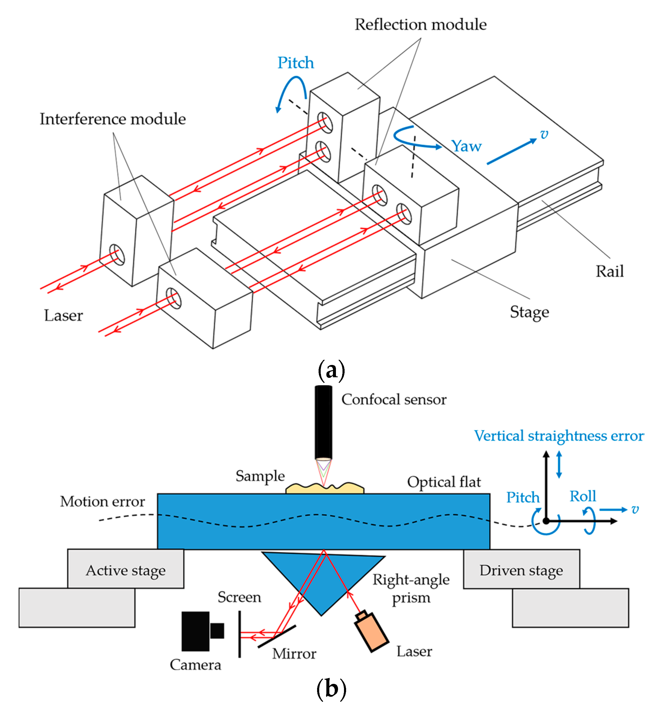
Another motivation of the presented work was to develop an interferometric system, which was able to quantify and compensate the motion error from the bottom of the 3D surface topography measurement instrument [26]. Traditional laser interferometric systems, based on the Michelson principle, are usually used for measuring one-dimensional angular motion errors (yaw or pitch) during the movement of the stage [27,28], as shown in Figure 1a. In order to measure multi-degree-of-freedom motion errors at the same time, more than one interferometric module is required. Furthermore, yaw has no effect on the height measurement, so it is less critical in topography measurement. The film interferometer, presented in this paper, is capable of measuring straightness errors in the vertical direction and angular values (yaw and roll) simultaneously, which directly affect the height measurement, as shown in Figure 1b. If a traditional Michelson interferometer was built to meet this requirement, a flawless reflective mirror would be needed to cover the entire measurement area. Such large mirrors with perfect flatness and surface quality are not practically available. In the presented work, optical flats, with very affordable flatness references, were used to generate the interferogram. Further, image processing based on areal sampling was able to effectively minimize the impact of surface imperfections.
In summary, the motivation of this study was to develop a straightness measurement system, which was not only able to verify a motion system but also to improve the accuracy for topography measurement with reasonable cost and respectable robustness. Being applied in an in-house-developed topography measurement system, the proposed methodology was proven by significantly improving the measurement accuracy [26]. In this paper, details on the optical scheme, image quality, implementation method, error factors, and system robustness were disclosed.
2. Principle of Film Interference Module
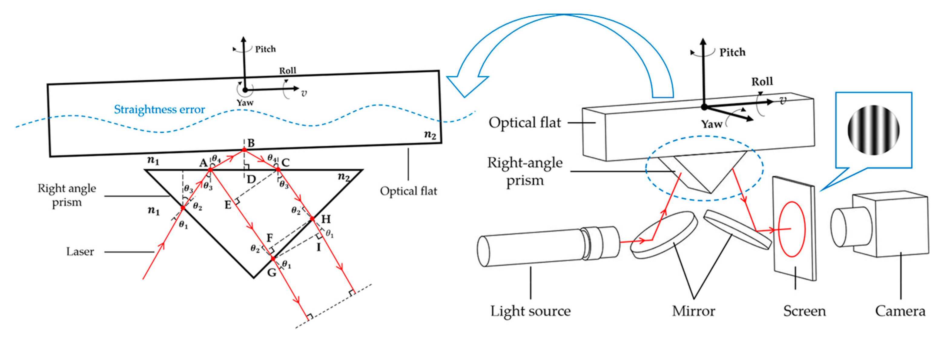
In order to provide detailed information on the development work, the principle, calibration process, and data analysis were discussed based on a standalone experimental setup, as shown in Figure 2.
The experimental system mainly included an optical flat and a right-angle prism. The optical flat was a datum mounted on a precision linear stage under test and formed an air wedge with a stationary right-angle prism. The angle of the air wedge was very small, usually within 100″. With a proper incident direction, the light source was split into two beams and reflected with the same propagation path approximately, and a film interferogram could be observed on the screen. During the movement of the optical flat, the interferogram would show a phase shift according to the thickness variation of the air wedge, which was directly related to the straightness error of the linear stage. Therefore, the straightness error could be measured based on the phase shift of the interferogram.
As shown in Figure 2, the optical path difference between the two interfering light beams can be expressed as:
where n1 and n2 are the refractive indexes of the air and optical glass, respectively. Since the angle and thickness of the air wedge were very small, AB was approximately equal to BC:
So Equation (1) can be modified as:
Set GH = a, HI and FG can be obtained through geometric relationships:
The right half of Equation (3) can be calculated:
The distance between the two interference surfaces was set as BD = h, so the optical path difference d can be expressed as:
According to Equation (7), Equation (9) can be further simplified:
Equation (10) is the classic optical path difference formula for the parallel air wedge. Substituting Equations (6) and (7) into Equation (10), which can be modified as:
Since the refractive indexes of the optical flat and the right-angle prism were the same in the system, the half-wave rectification caused by reflection must be considered:
The relationship between the change in the optical path difference Δd and the change in distance Δh (straightness error) can be expressed as:
When the phase shift of the interferogram Δφ was equal to 2π (one wave cycle), the optical path difference would be changed by one wavelength. Hence, the phase shift Δφ was linearly correlated with the optical path Δd:
The conditional parameters, including wavelength λ, the refractive indexes n1 and n2, and the incident angle θ1 were independent with the phase shift Δφ. Hence, the item before Δh can be substituted by a constant c:
And Equation (14) can be modified as:
Equation (16) shows that the magnitude and direction of the straightness error Δh can be calculated by dividing the phase shift Δφ of the interferogram by the linear coefficient c.
3. Analysis of Angular Motion Error
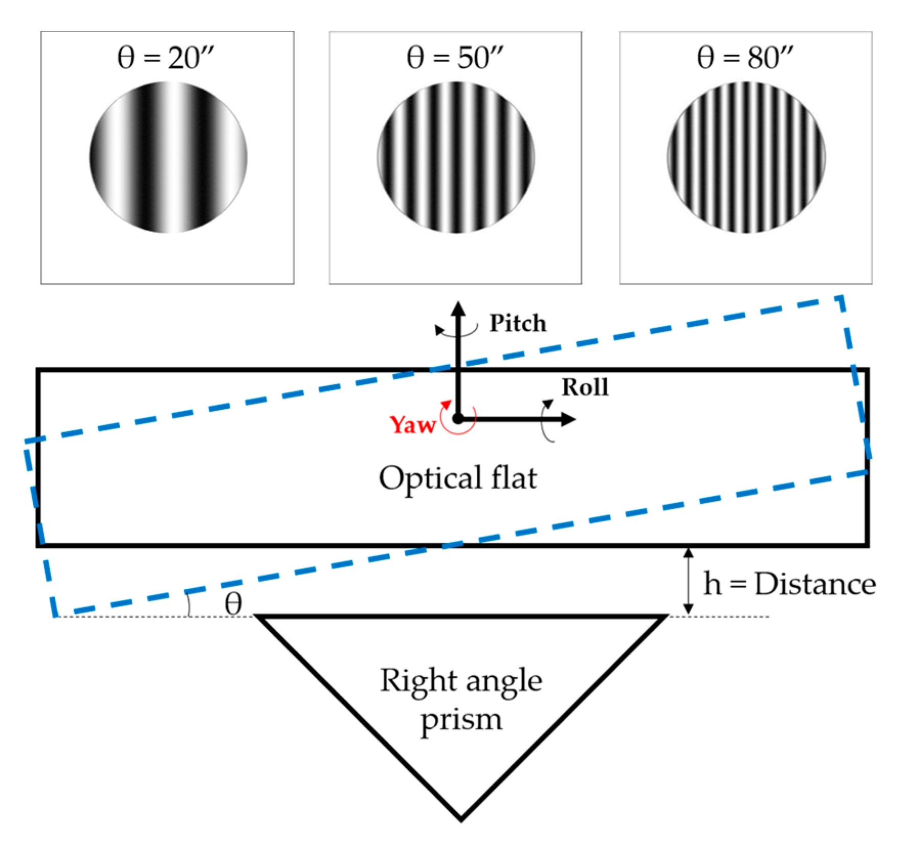
Straightness error can be expressed either in linear values (in microns or nanometers) or angular values (in arcseconds or microradians). The present work was focused on linear values. According to the analysis in the above section, c is irrelevant with the angle of the air wedge affected by angular motion error. In order to verify the conclusion, a simulation-based on ZEMAX was conducted.
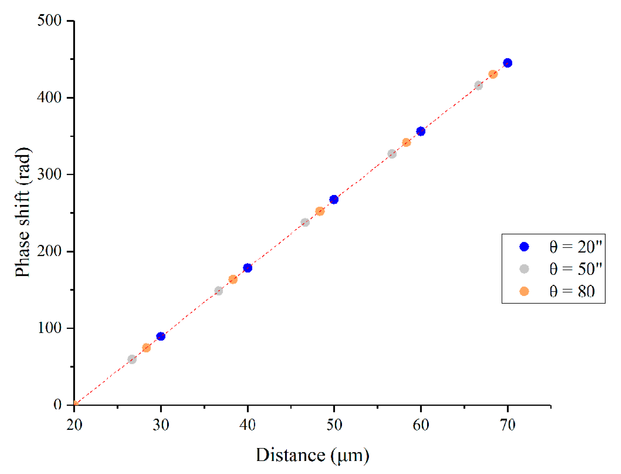
In general, the angular motion error of a precision linear stage can be well controlled within 60″, so the setting of θ to be 20″, 50″, and 80″ was sufficient to simulate the impact of the angular motion error. As shown in Figure 3, the angular motion error affected the spacing and orientation of the interferogram. Figure 4 shows that the relationship between the distance and phase shift remained consistent with a different set of angles. As shown in Table 1, the linear coefficient c was independent of the preset angle. Therefore, the angular motion error was a separate topic and did not affect the linear straightness measurement method proposed in this paper, at least within the operational range.
Therefore, it could be concluded that, although the angular motion error varied in the appearance of the interferogram, it did not affect the mathematical model.
4. Phase Calculation Based on Image Processing
The direct mathematical calculation of the phase shift Δφ was challenging due to the imperfection of the interferogram. In this study, the phase shift Δφ was determined by an image processing algorithm.
4.1. Analysis of the Cause of Fringe Distortion
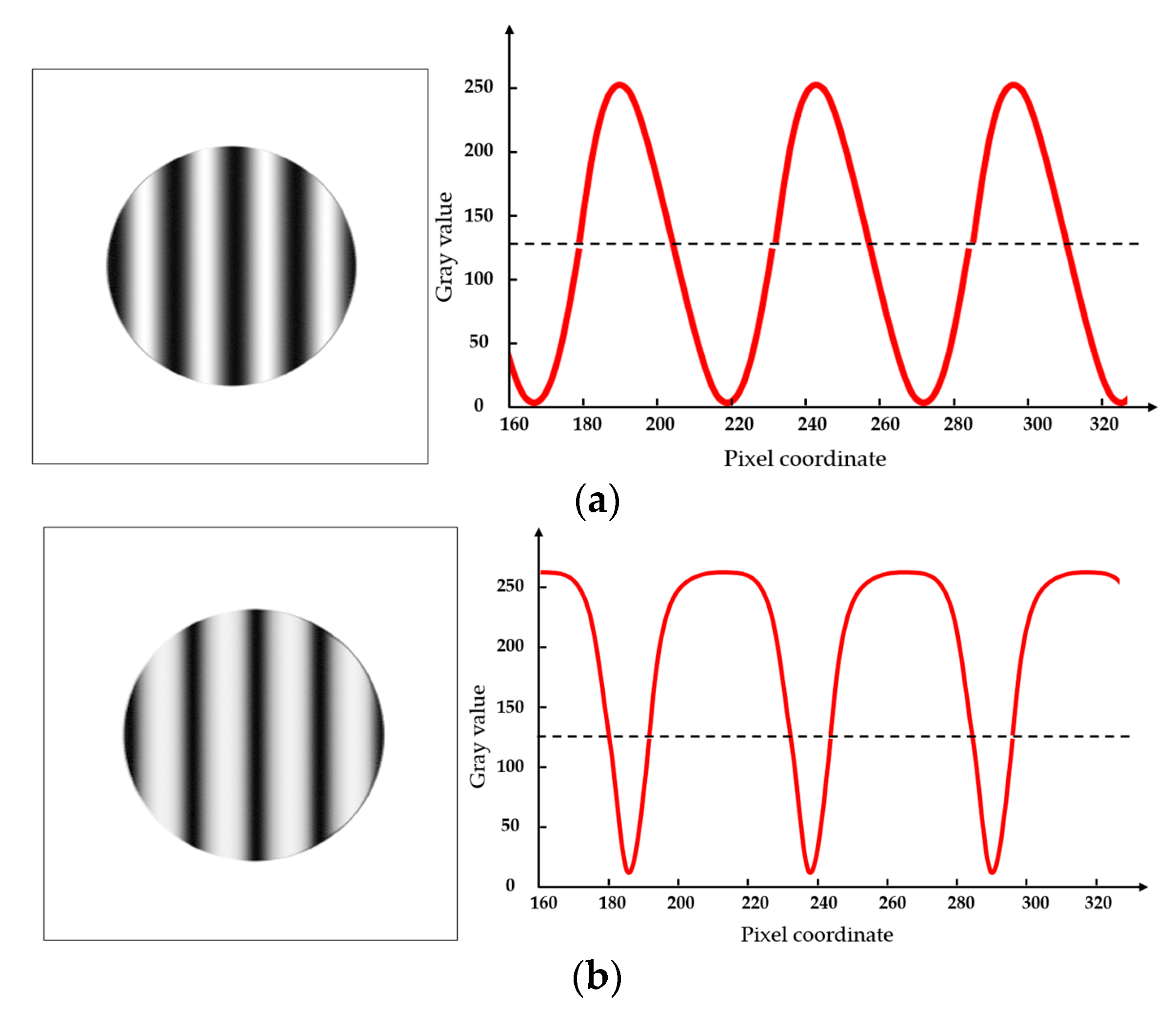
Assuming the incident light was reflected only once by each optical surface, a two-beam interferogram would be generated. Figure 5a shows the ZEMAX simulation results of the two-beam scenario. The grayscale variation showed an ideal sinusoidal pattern. In this ideal scenario, the phase information could be easily obtained by methods such as the Fourier transform. However, in the actual experiments, the interferogram generated by the actual optics showed multi-beam patterns. The incident light was reflected more than once between the two optical surfaces. When the multi-beam reflection was set as the initial condition for the ZEMAX simulation, the interferogram showed a significant skewness, as shown in Figure 5b.
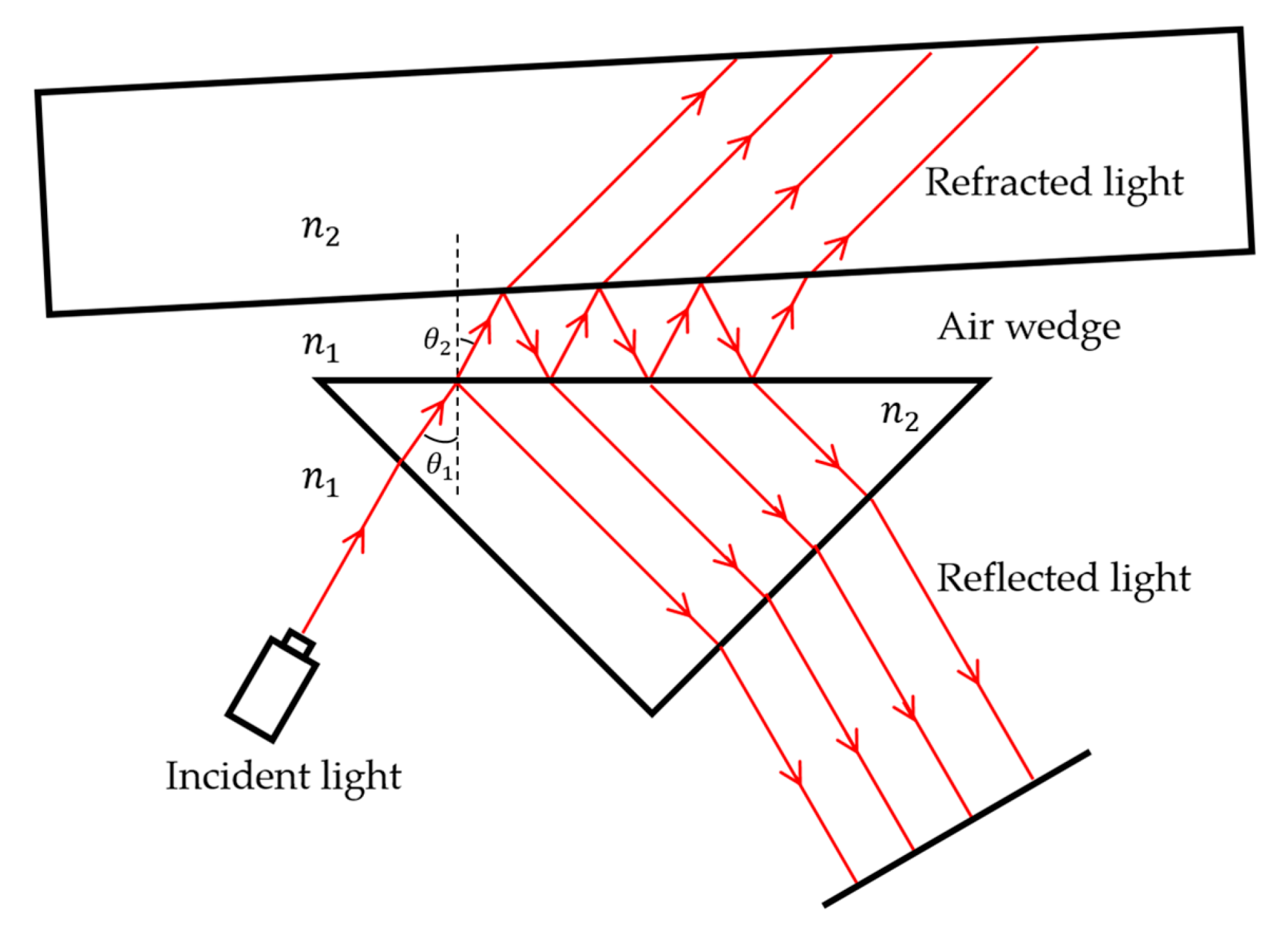
As discussed in the above paragraphs, the root cause of the waveform distortion was the multi-reflection that occurred in the air wedge, as illustrated in Figure 6.
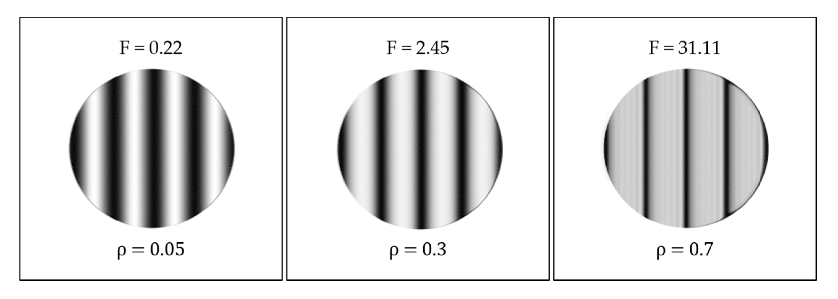
The waveform distortion, due to multi-reflection, could be quantitatively expressed by the coefficient of finesse F [30]:
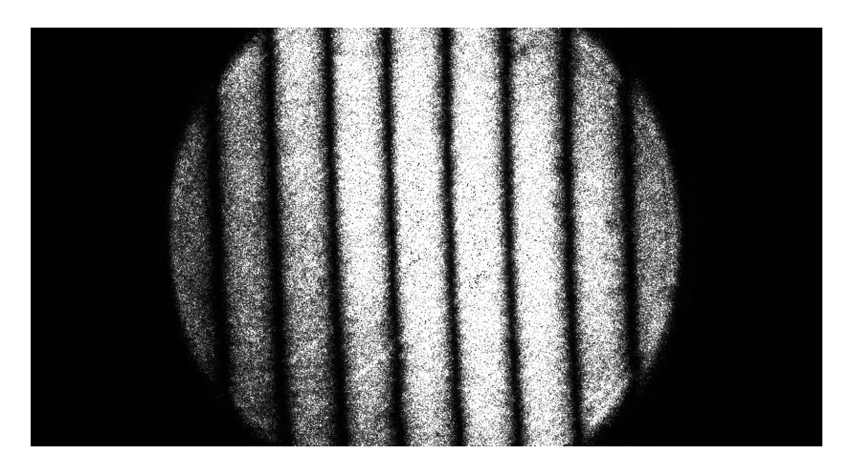
where ρ is the interface reflectance. According to Equation (17), a higher value of ρ will result in a higher value of F. With the finesse F increasing, the stripes become finer, and their edges become sharper. This correlation was represented by wider bright stripes in the interferogram generated by the ZEMAX simulation, as shown in Figure 7. The actual image captured from the experimental system was consistent with the simulation and mathematical analysis, as shown in Figure 8.
4.2. Edge Extraction and Phase Calculation
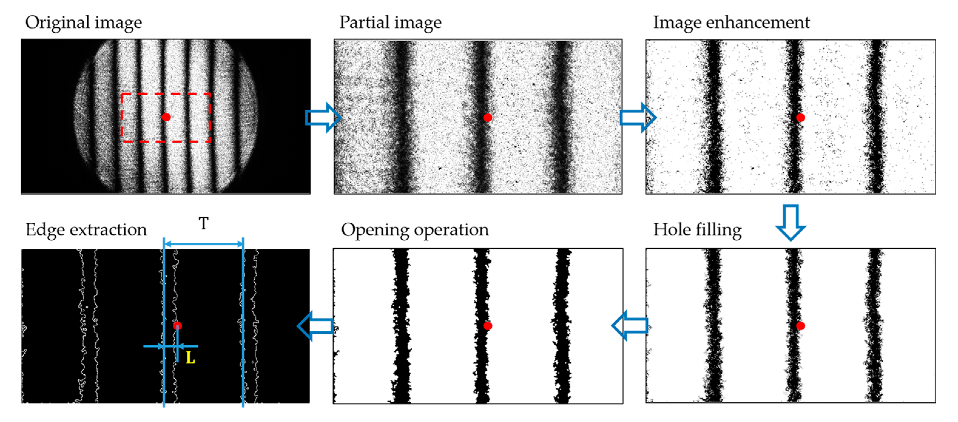
In this study, interferograms were captured continuously during the movement of the optical flat. The phase values were calculated in real-time. Due to the multi-beam interference, the fringes showed sharp edges. Therefore, edge detection technology was applied to identify the interference signal, as shown in Figure 9:
Step 1. Central area selection to minimize the optical distortion from the imaging system.
Step 2. Image enhancement to improve the image contrast.
Step 3. Hole filling to patch the holes induced by the binarization process.
Step 4. Opening operation to reduce the noise at the edges and separate edges of neighboring fringes.
Step 5. Edge extraction to store edge information in the format of pixel arrays.
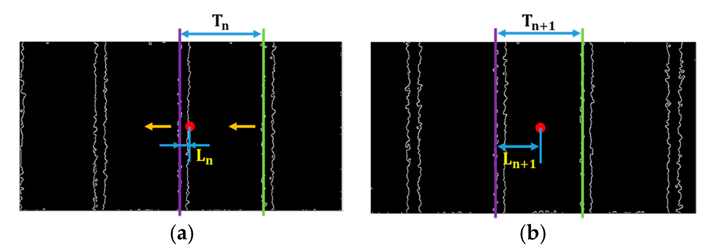
The red dot in Figure 9 represents the location for straightness measurement. If the fringe edge is on the left side of the dot, the distance L is a positive number; otherwise, it is negative. As shown in Figure 10, assuming that the phase of the first interferogram φ1 is 0, and the phase of the nth interferogram was φn, then the phase of the (n + 1)th interferogram φn+1 can be expressed as:
Transforming Equation (18) to obtain the phase difference Δφn:
5. Experimental Analysis
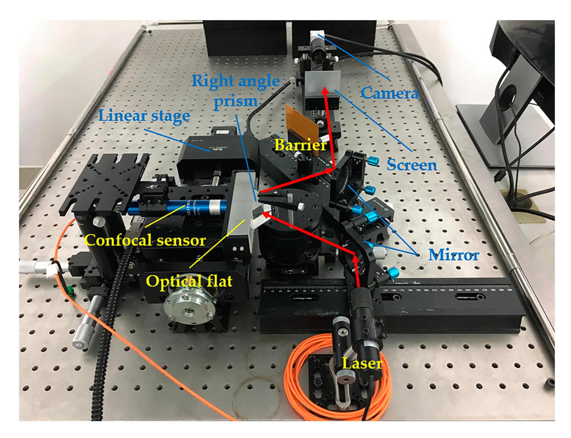
In order to verify the proposed method, the experimental tests were conducted with the system shown in Figure 11. The key components with the specifications are listed in Table 2.
The optical flat was mounted on the linear stage as a geometric reference and formed an air wedge with the stationary right-angle prism. The two mirrors were used to adjust the incident light. The linear stage was driven by an MC600 controller (Zolix Instruments Co., Ltd., Beijing, China). During the stage movement, interferogram images were captured at 51 locations with an increment of 1 mm. The confocal sensor was used as a reference for calibration and comparison. Since only about 5% of the measurement range was used, it could be considered that the nonlinearity error in this range was insignificant.
5.1. System Calibration
Before verifying the straightness error measurement capability of the film interferometer, the linear coefficient c was determined. From Equation (15), c was mainly affected by the wavelength λ of the incident beam, the refractive indexes n1 and n2, and the incident angle θ1. It was difficult to obtain the four parameters accurately. In this study, therefore, c was determined experimentally. By precisely adjusting the distance between the two optical surfaces with known positions, the coefficient c could be obtained.
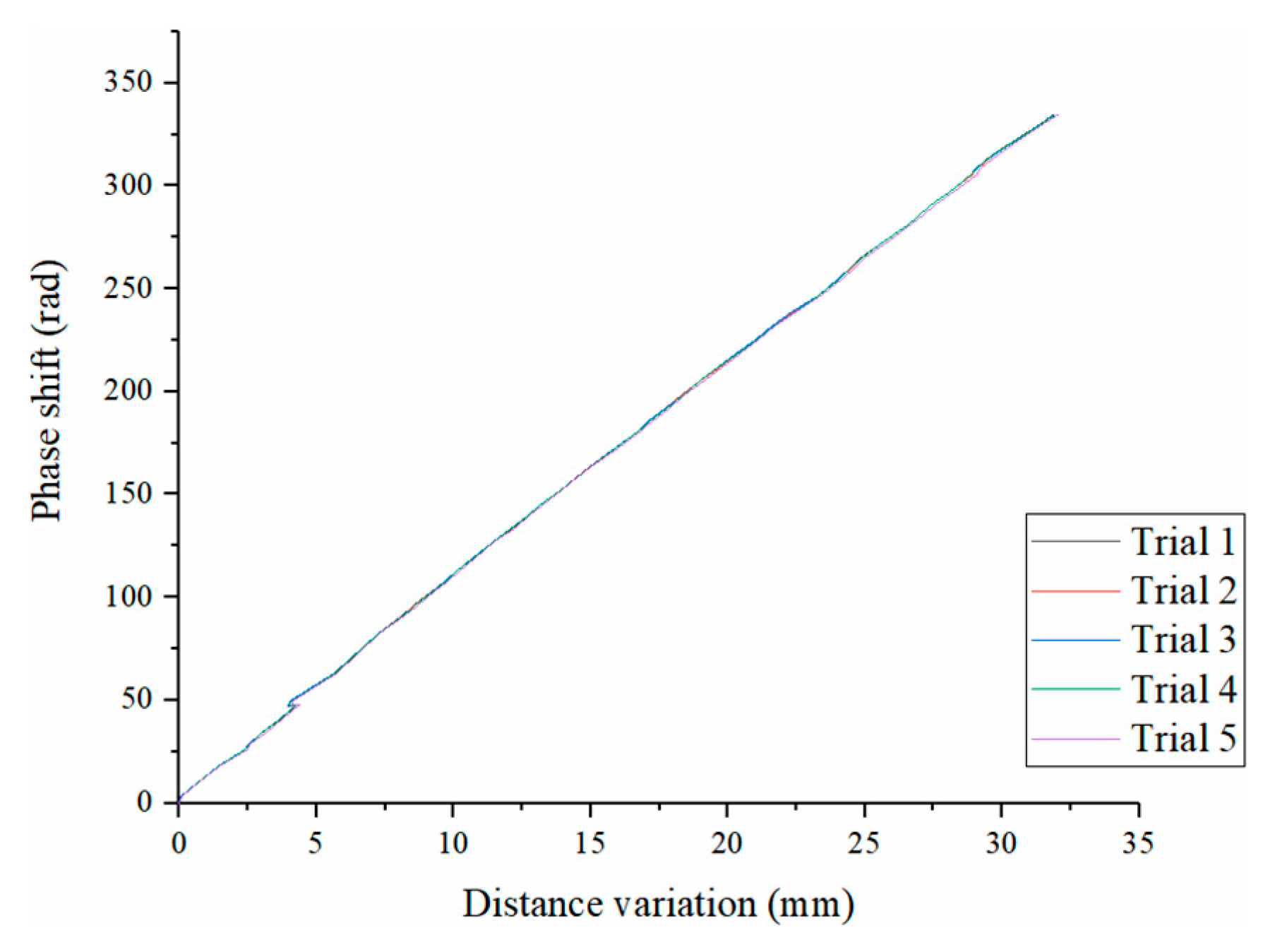
The measurements were repeated five times. As shown in Figure 11, the confocal sensor was used to record the change in distance Δh. Assuming that the measurement lo-cation of the film interferometer was in the center of the image (1024, 544), the phase shift of the interferogram Δφ was calculated by the developed image processing algorithm, as introduced in Section 4.2. Then the relationship between distance variation and phase shift was obtained, as shown in Figure 12. The phase shift was approximately linear with the distance variation, which was consistent with the theoretical analysis (in Section 2) and simulation (in Section 3). The linearity coefficient c was calculated by averaging the five slope values, as shown in Table 3. The standard deviation of c was about 0.1% of the average.
The c value calculated from Table 3 was slightly different from the theoretical value from Table 1. The main root causes of this deviation included the deviation of the actual angle θ1 against the ideal setting and the imperfection of the optical components.
After the calibration, the relationship between Δφ and Δh could be obtained according to Equation (16):
5.2. Measurement Performance
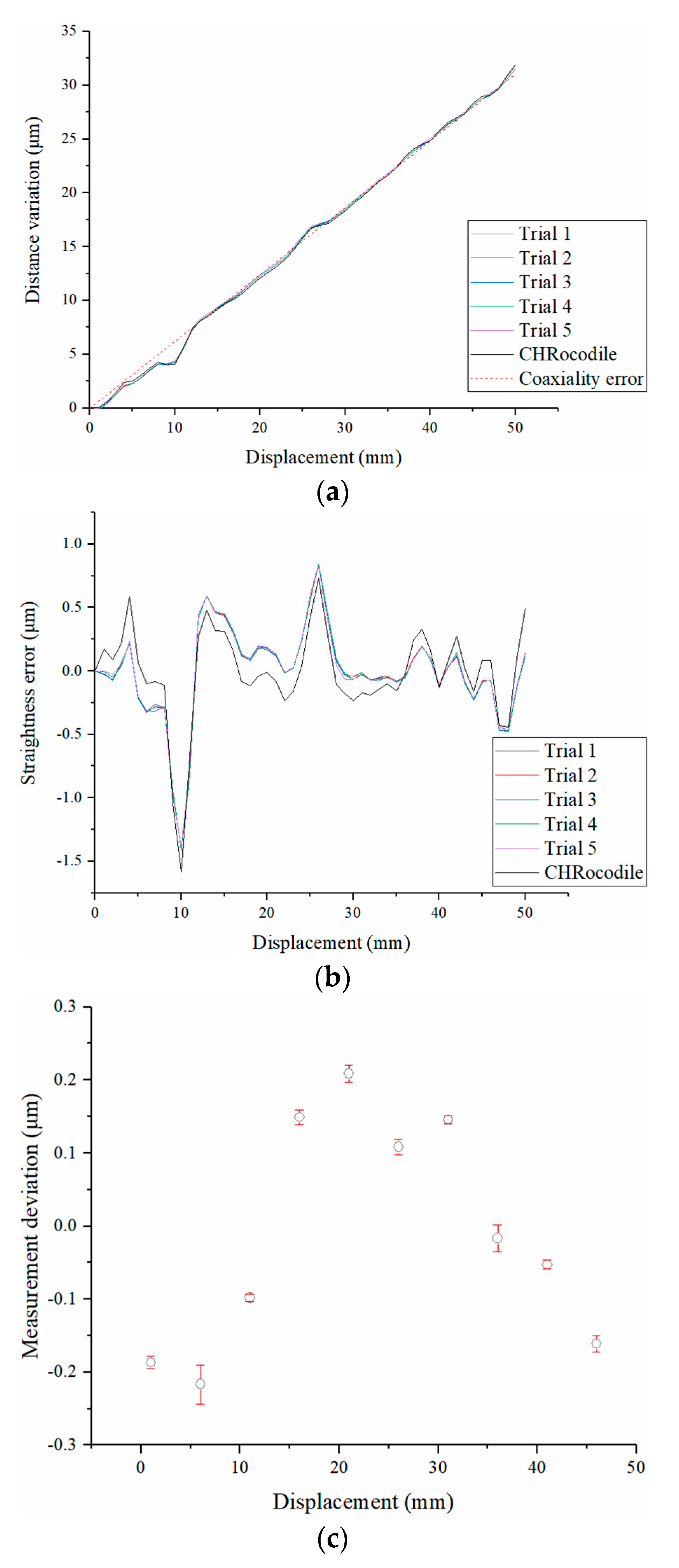
When the linear relationship was determined, the variation of the distance between the two optical surfaces was calculated by analyzing the phase shift of each interferogram. The confocal sensor was applied as a reference sensor. The comparison of the measurement results was shown in Figure 13a. During the assembly process, it was difficult to ensure that the optical flat was strictly parallel to the ideal moving axis. This parallelism error resulted in a linear increase (or decrease) in the thickness of the air wedge. This thickness variation was superimposed with the straightness error, as shown in Figure 13a, and could be removed by the linear fitting process, as shown in Figure 13b. The data of five repeats showed a strong correlation. As shown in Figure 13c, the measurement deviation between the film interferometer and the reference confocal sensor was within ±0.22 μm. In the travel range of 50 mm, the standard deviation was within 25 nm.
5.3. Analysis of the Source of Measurement Deviation
In this study, there were three main error sources: measurement equipment, measurement process, and measurement environment. In this section, the error source analysis and measurement accuracy improvement were discussed.
- (1)
- Measurement equipment
As shown in Table 2, the flatness of the right-angle prism and the optical flat were 0.06 μm and 0.05 μm, respectively. Hence, the systematic error caused by the imperfection of the two optical elements might reach up to a submicron level theoretically. Secondly, the confocal sensor used as the reference had its own measurement errors, such as nonlinearity errors.
- (2)
- Measurement process
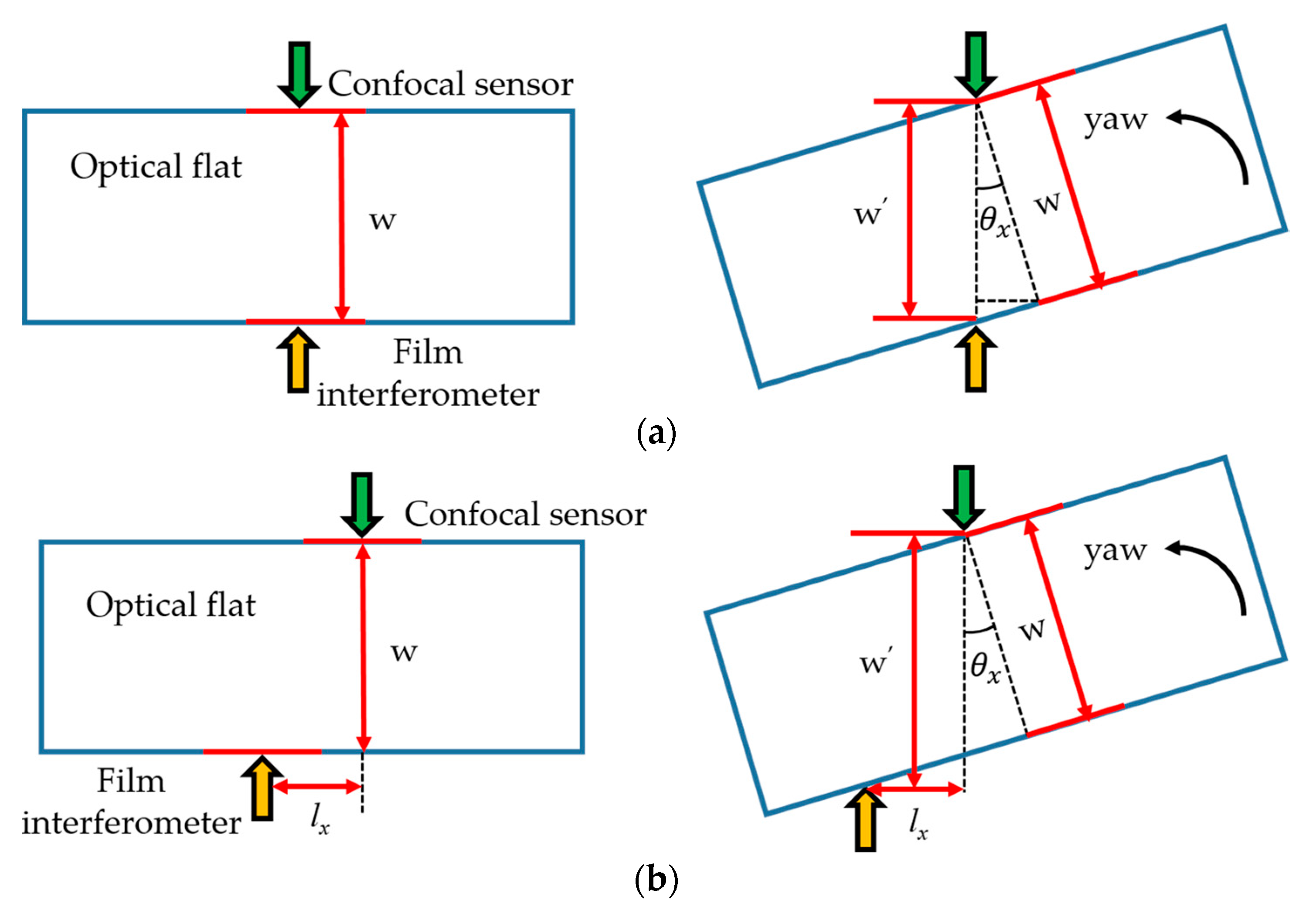
In the measurement process, the misalignment of the measurement locations of the film interferometer and the reference confocal sensor was very critical. Figure 14 shows the impact of the misalignment.
During the movement of the linear stage, the angular motion error was inevitable. As described in Section 2 and Section 3, the angular motion error did not affect the linearity coefficient c, but it varied the distance between the measurement locations of the confocal sensor and the film interferometer, resulting in a measurement deviation.
As shown in Figure 14a, when the measurement locations were well aligned, the measurement deviation due to the angular motion error θx (θx → 0) could be expressed as:
According to Equation (22), the measurement deviation Δx is the infinitesimal of a higher order of angular error θx. It indicated that the measurement deviation caused by the angular error was insignificant when the measurement locations were properly aligned.
As shown in Figure 14b, when the measurement locations of the confocal sensor and the film interferometer were not aligned horizontally (the horizontal distance is lx), the measurement deviation would be different from the above scenario:
As shown in Equation (24), the measurement deviation Δx is the infinitesimal of the same order of angular error θx. It means that the impact of the angular error was significant. Therefore, in order to accurately evaluate the straightness error measurement capability of the film interferometer, it was necessary to ensure that the measurement locations of the film interferometer and the confocal sensor were aligned horizontally and vertically.
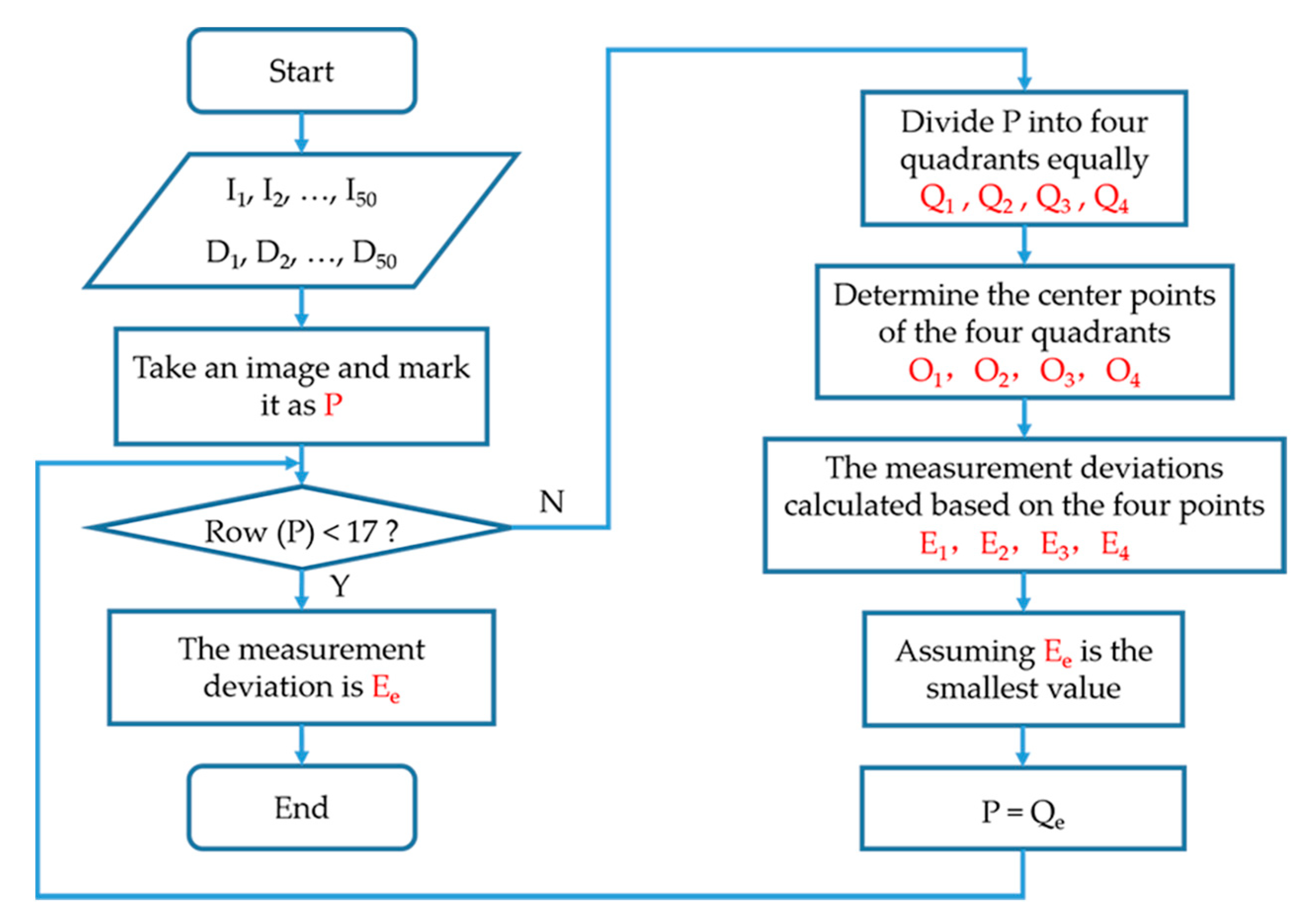
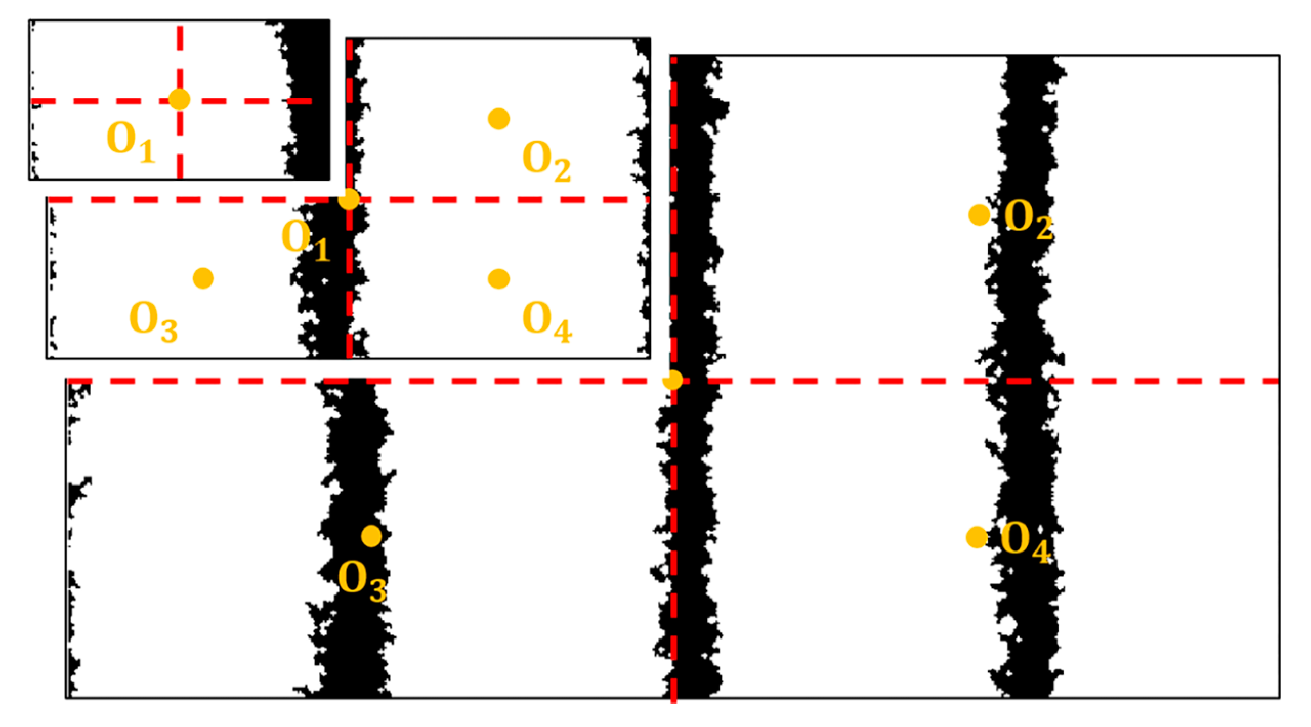
Figure 15 and Figure 16 show the method to ensure the proper alignment. I1, I2, …, I50 were the 50 interferograms captured by the camera, and D1, D2, …, D50 were the distance variation measured by the confocal sensor.
When the image processing algorithm was executed, every image (the fifth in Figure 9) was equally divided into four quadrants—Q1, Q2, Q3, Q4—and their center points—O1, O2, O3, O4—were determined, respectively. Taking these four centers as the measurement locations of the film interferometer, four measurement deviation results—E1, E2, E3, E4—could be obtained. Comparing the four values, assuming E1 was the minimum value, then O1 was the closest to the optimal measurement location among the four center points. In other words, the optimal measurement location was in Q1. Subsequently, Q1 was further divided into four quadrants, and the above process was repeated. After several iterations, the measurement location could be sufficiently close to the optimal location.
Therefore, in this study, the alignment process did not require any physical adjustment. The alignment process was actually the selection of the optimal measurement point in the image. Compared with the single point sensing methods, such as LVDT (Linear Variable Differential Transformer), the assembly and adjustment processes were much simpler.
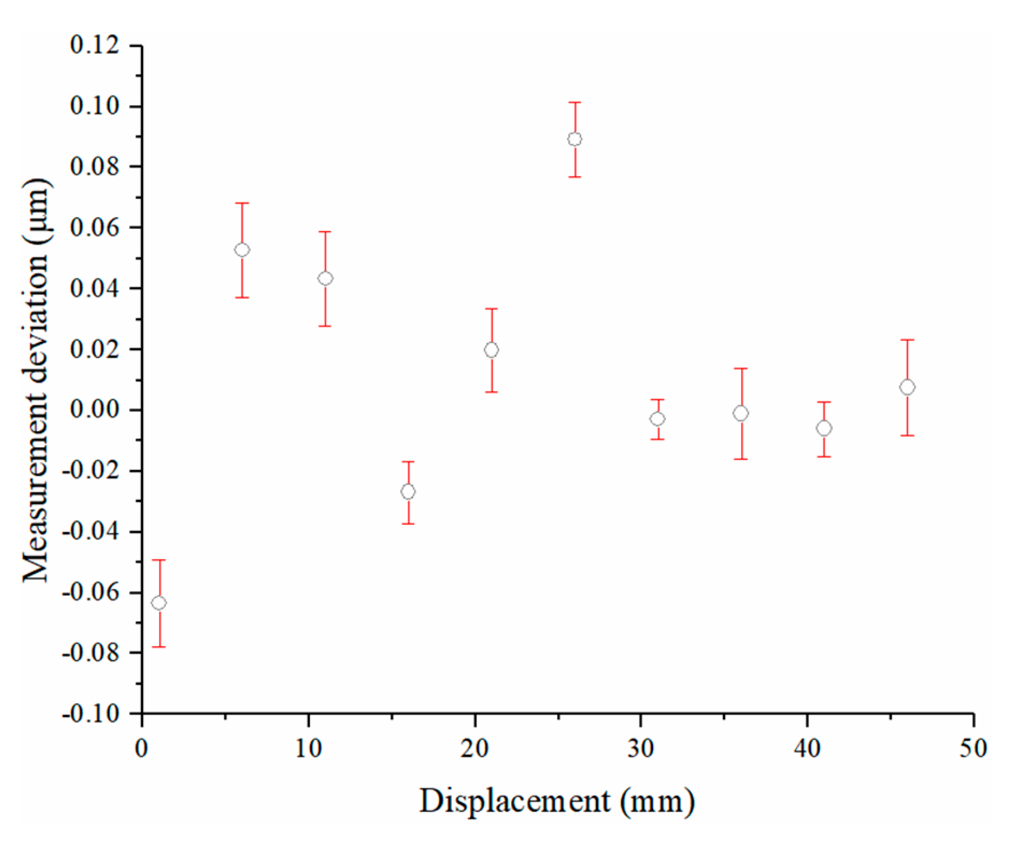
After identifying the optimal measurement location, the same experiments in Section 5.2 were performed again. The experimental data are shown in Figure 17. The measurement deviation between the film interferometer and the reference confocal sensor was reduced to ±0.1 μm, which indicated a significant improvement, as compared to ±0.22 μm shown in Figure 13c. Five repeats were performed at each location. The standard deviation was within 25 nm.
Considering the imperfect flatness of the optical flat and the inherent measurement error from the confocal sensor, ±0.1 µm was a conservative accuracy statement of the development system.
It’s worth highlighting that this process of selecting the optimal measurement location was critical for not only the calibration process but also the actual measurement when setting up the film interferometer into a topography measurement shown in Figure 1b. In actual topography measurement, the main probe measuring the height would take the place of the reference confocal sensor shown in Figure 11. The film interferometer should be able to quantify and compensate for the motion error that occurred in the axial direction of the main probe.
- (3)
- Measurement environment
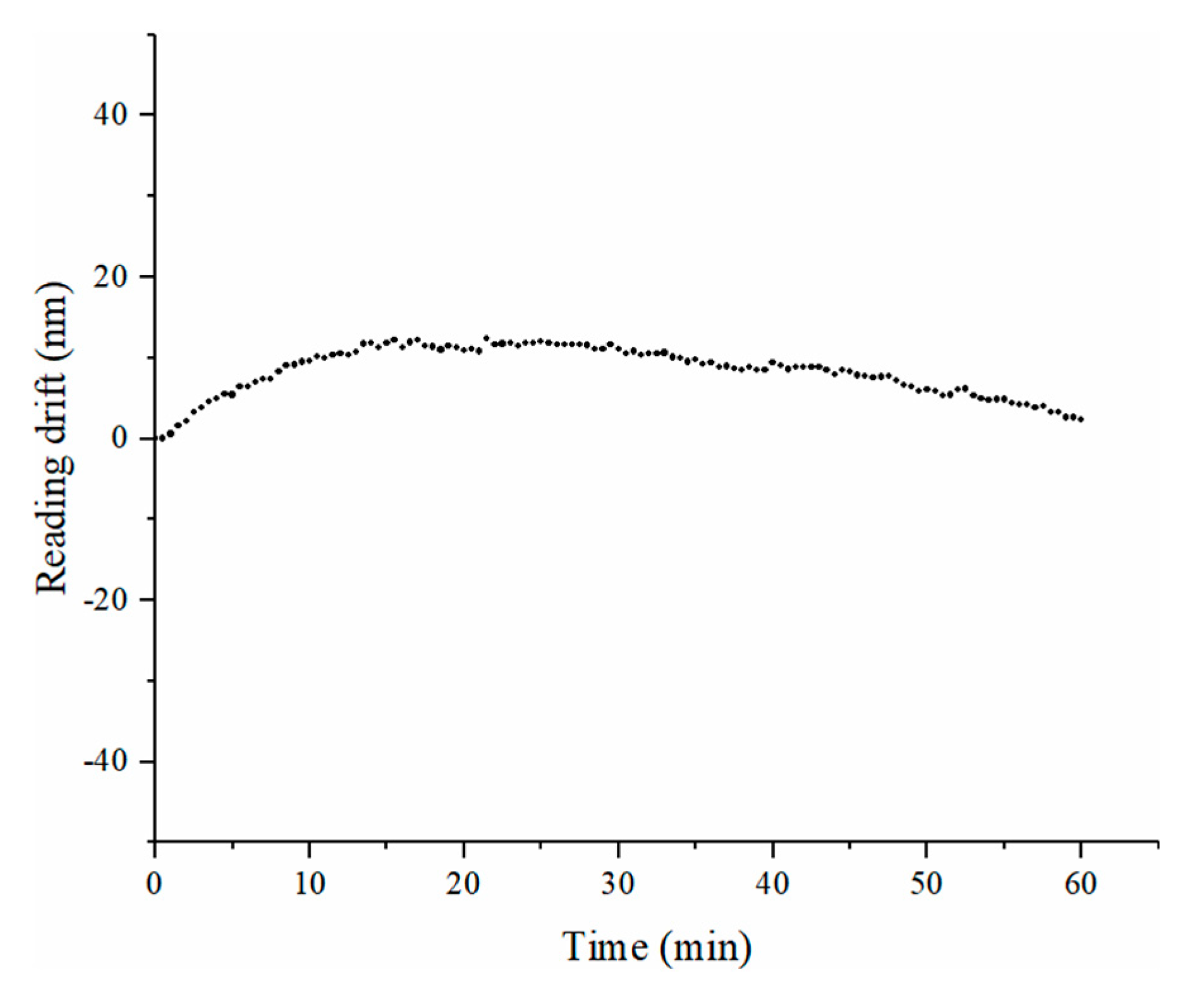
The temperature was a concern for most interferometric measurement techniques. A temperature drift experiment was performed to verify the environment robustness of the film interferometer. The film interferometer was placed in a common air-conditioned environment for one hour, and the camera was set to take an interferogram every 30 s. Based on the phase analysis algorithm described in Section 4.2, the measurement reading drift was obtained. As shown in Figure 18, the reading drift of the film interferometer was within 12 nm in one hour when the temperature varied between 18 °C and 22 °C.
6. Conclusions
In this paper, a film interferometer for measuring the straightness error of a precision motion system was proposed. The principle of the film interference module and phase calculation process were discussed. In the presented system, an optical flat and a right-angle prism were used to generate the interferogram. An image processing method was applied to calculate the phase shift induced by the straightness error. The components used in this system were widely available and affordable in the market. In addition, compared with traditional interferometric systems, the presented system was also featured by its easy alignment process and good environmental robustness.
Experimental tests were performed to verify the straightness error measurement capability of the developed film interferometer. The experimental results showed that the measurement deviation between the proposed system and the reference sensor was better than ±0.1 μm, and the repeatability, represented by the standard deviation, was within 20 nm in a travel range of 50 mm.
This system is potentially able to measure the straightness in both linear and angular values online. At present, the main focus is on the analysis of its linear value measurement capability. The new capability of measuring the angular motion error is also under development.
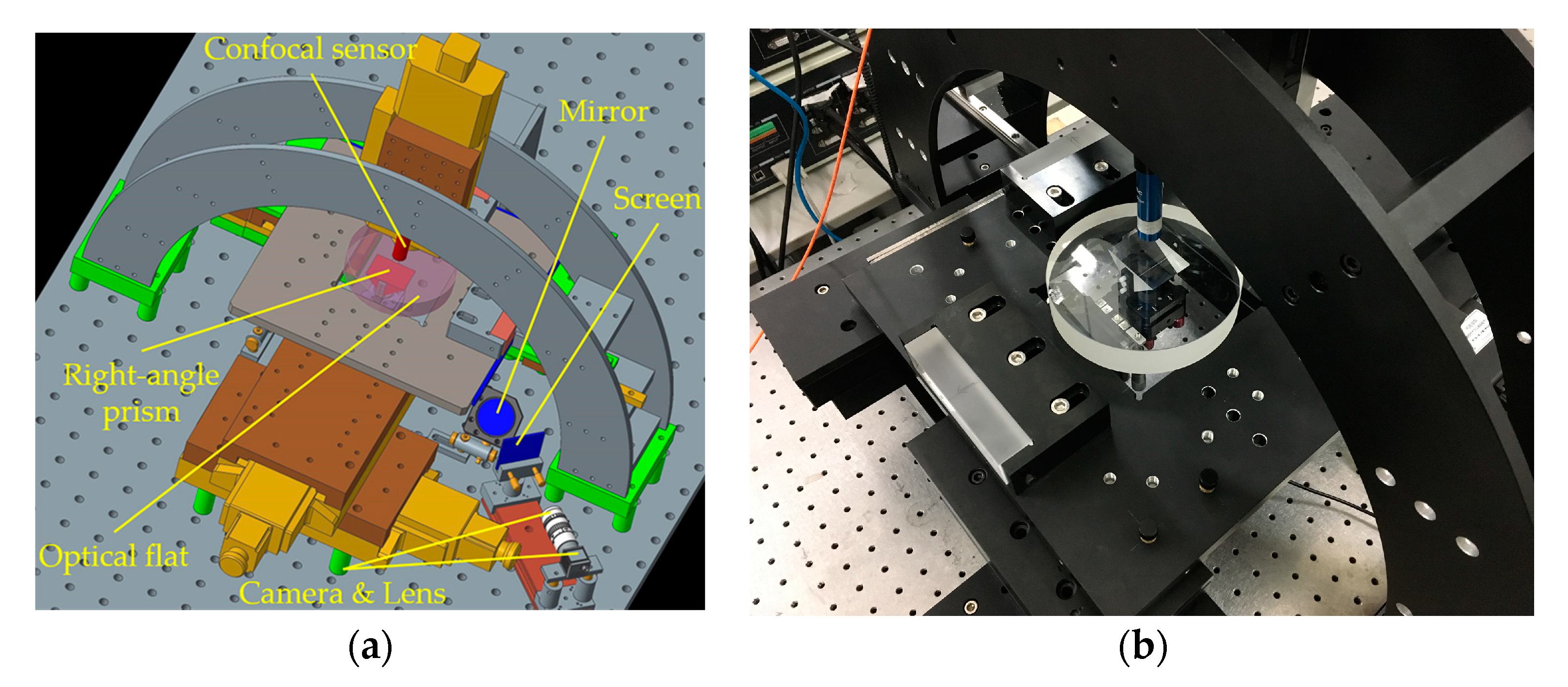
This proposed film interferometer was successfully implemented in a 3D surface topography measurement system developed by the authors’ team, as shown in Figure 19. In that system, the film interferometer was used to compensate for the motion error. With effective error compensation, the 3D surface topography measurement system was able to achieve repeatability and reproducibility within 0.1 µm. The objective of publishing this paper was to provide more details of the film interferometer, which was applied as a subsystem in the work published earlier.
Author Contributions
Conceptualization, F.C.; methodology, F.C.; software, H.S.; validation, R.Y., F.C., C.C. and Q.Y.; formal analysis, H.S., R.Y. and F.C.; investigation, H.S. and R.Y.; resources, R.Y. and F.C.; data curation, H.S. and R.Y.; writing—original draft preparation, H.S. and R.Y.; writing—review & editing, H.S., R.Y., F.C., C.C. and Q.Y.; visualization, H.S. and F.C.; supervision, R.Y. and F.C.; project administration, R.Y. and F.C.; funding acquisition, H.S., R.Y. and F.C. All authors have read and agreed to the published version of the manuscript.
Funding
This research was funded by the Fundamental Research Funds for the Central Universities, China (ZQN-703); the National Natural Science Foundation of China (Grant No. 51605171); the National Natural Science Foundation of China (Grant No. 52075190); and the Subsidized Project for Postgraduates’ Innovative Fund in Scientific Research of the Huaqiao University (Grant No. 18013080058).
Institutional Review Board Statement
Not applicable.
Informed Consent Statement
Informed consent was obtained from all subjects involved in the study.
Data Availability Statement
Data available in a publicly accessible repository.
Acknowledgments
The authors would like to thank LetPub (www.letpub.com, accessed on 19 April 2021) for its linguistic assistance during the preparation of this manuscript and all reviewers for their helpful comments and suggestions.
Conflicts of Interest
The authors declare no conflict of interest.
References
- Jin, T.; Ji, H.; Hou, W.; Le, Y.; Shen, L. Measurement of straightness without Abbe error using an enhanced differential plane mirror interferometer. Appl. Opt. 2017, 56, 607–610. [Google Scholar] [CrossRef]
- Lai, T.; Peng, X.; Liu, J.; Tie, G.; Meng, G. High accurate measurement and calibration of the squareness on ultra-precision machine based on error separation. Proc. Inst. Mech. Eng. Part B 2019, 233, 600–609. [Google Scholar] [CrossRef]
- Huang, S.H.; Pan, Y.C. Automated visual inspection in the semiconductor industry: A survey. Comput. Ind. 2015, 66, 1–10. [Google Scholar] [CrossRef]
- Kim, Y.S.; Yoo, J.M.; Yang, S.H.; Choi, Y.M.; Dagalakis, N.G.; Gupta, S.K. Design, fabrication and testing of a serial kinematic MEMS XY stage for multifinger manipulation. J. Micromech. Microeng. 2012, 22, 85029. [Google Scholar] [CrossRef] [Green Version]
- Nouira, H.; El-Hayek, N.; Yuan, X.; Anwer, N. Characterization of the main error sources of chromatic confocal probes for dimensional measurement. Meas. Sci. Technol. 2014, 25, 044011. [Google Scholar] [CrossRef]
- Hsieh, T.H.; Chen, P.Y.; Jywe, W.Y.; Chen, G.W.; Wang, M.S. A geometric error measurement system for linear guideway assembly and calibration. Appl. Sci. 2019, 9, 574. [Google Scholar] [CrossRef] [Green Version]
- Chai, N.; Yin, Z.; Yao, J. High Accuracy Profile Measurement with a New Virtual Multi-Probe Scanning System. IEEE Access. 2020, 8, 158727–158734. [Google Scholar] [CrossRef]
- Weichert, C.; Bosse, H.; Flügge, J.; Köning, R.; Köchert, P.; Wiegmann, A.; Kunzmann, H. Implementation of straightness measurements at the Nanometer Comparator. CIRP Ann. Manuf. Technol. 2016, 65, 507–510. [Google Scholar] [CrossRef]
- Küng, A.; Bircher, B.A.; Meli, F. Low-Cost 2D Index and Straightness Measurement System Based on a CMOS Image Sensor. Sensors 2019, 19, 5461. [Google Scholar] [CrossRef] [Green Version]
- Fung, E.H.K.; Zhu, M.; Zhang, X.Z.; Wong, W.O. A novel Fourier-Eight-Sensor (F8S) method for separating straightness, yawing and rolling motion errors of a linear slide. Measurement 2014, 47, 777–788. [Google Scholar] [CrossRef]
- Fan, K.C.; Chen, M.J. A 6-Degree-of-freedom measurement system for the accuracy of X-Y stages. Precis. Eng. 2000, 24, 15–23. [Google Scholar] [CrossRef]
- Yu, X.; Gillmer, S.R.; Woody, S.C.; Ellis, J.D. Development of a compact, fiber-coupled, six degree-of-freedom measurement system for precision linear stage metrology. Rev. Sci. Instrum. 2016, 87, 065109. [Google Scholar] [CrossRef] [Green Version]
- Gao, W.; Arai, Y.; Shibuya, A.; Kiyono, S.; Parke, C.H. Measurement of multi-degree-of-freedom error motions of a precision linear air-bearing stage. Precis. Eng. 2006, 30, 96–103. [Google Scholar] [CrossRef]
- Hsieh, H.L.; Pan, S.W. Development of a grating-based interferometer for six-degree-of-freedom displacement and angle measurements. Opt. Express 2015, 23, 2451–2465. [Google Scholar] [CrossRef] [PubMed]
- Borisov, O.; Fletcher, S.; Longstaff, A.; Myers, A. New low cost sensing head and taut wire method for automated straightness measurement of machine tool axes. Opt. Laser Eng. 2013, 51, 978–985. [Google Scholar] [CrossRef] [Green Version]
- Lee, H.W.; Liu, C.H. High precision optical sensors for real-time on-line measurement of straightness and angular errors for smart manufacturing. Smart Sci. 2016, 4, 134–141. [Google Scholar] [CrossRef]
- Cai, Y.; Lou, Z.; Ling, S.; Liao, B.; Fan, K. Development of a compact three-degree-of-freedom laser measurement system with self-wavelength correction for displacement feedback of a nanopositioning stage. Appl. Sci. 2018, 8, 2209. [Google Scholar] [CrossRef] [Green Version]
- Gao, W.; Saito, Y.; Muto, H.; Arai, Y.; Shimizu, Y. A three-axis autocollimator for detection of angular error motions of a precision stage. CIRP Ann. Manuf. Technol. 2011, 60, 515–518. [Google Scholar] [CrossRef]
- Kimura, A.; Gao, W.; Zeng, L.J. Position and out-of-straightness measurement of a precision linear air-bearing stage by using a two-degree-of-freedom linear encoder. Meas. Sci. Technol. 2010, 21, 054005. [Google Scholar] [CrossRef]
- Yang, P.; Takamura, T.; Takahashi, S.; Takamasu, K.; Sato, O.; Osawa, S.; Takatsuji, T. Development of high-precision micro-coordinate measuring machine: Multi-probe measurement system for measuring yaw and straightness motion error of XY linear stage. Precis. Eng. 2011, 35, 424–430. [Google Scholar] [CrossRef]
- Chen, B.; Xu, B.; Yan, L.; Zhang, E.; Liu, Y. Laser straightness interferometer system with rotational error compensation and simultaneous measurement of six degrees of freedom error parameters. Opt. Express 2015, 23, 9052–9073. [Google Scholar] [CrossRef]
- Lu, Y.; Wei, C.; Jia, W.; Li, S.; Yu, J.; Li, M.; Xiang, C.; Xiang, X.; Wang, J.; Ma, J.; et al. Two-degree-freedom displacement measurement based on a short period grating in symmetric Littrow configuration. Opt. Commun. 2016, 380, 382–386. [Google Scholar] [CrossRef]
- Chen, B.; Cheng, L.; Yan, L.; Zhang, E.; Lou, Y. A heterodyne straightness and displacement measuring interferometer with laser beam drift compensation for long-travel linear stage metrology. Rev. Sci. Instrum. 2017, 88, 035114. [Google Scholar] [CrossRef]
- Zhu, L.Z.; Li, L.; Liu, J.H.; Zhang, Z.H. A method for measuring the guideway straightness error based on polarized interference principle. Int. J. Mach. Tool Manu. 2009, 49, 285–290. [Google Scholar] [CrossRef]
- Ye, W.; Zhang, M.; Zhu, Y.; Wang, L.; Hu, J.; Li, X.; Hu, C. Real-time displacement calculation and offline geometric calibration of the grating interferometer system for ultra-precision wafer stage measurement. Precis. Eng. 2019, 60, 413–420. [Google Scholar] [CrossRef]
- Cheng, F.; Zou, J.; Su, H.; Wang, Y.; Yu, Q. A differential measurement system for surface topography based on a modular design. Appl. Sci. 2020, 10, 1536. [Google Scholar] [CrossRef] [Green Version]
- Zhang, E.; Chen, B.; Zheng, H.; Teng, X.; Yan, L. Note: Comparison experimental results of the laser heterodyne interferometer for angle measurement based on the Faraday effect. Rev. Sci. Instrum. 2018, 89, 046104. [Google Scholar] [CrossRef]
- Kikuchi, G.; Furutani, R. Interferometer for pitch and yaw measurement using LC-screen and four ball lenses. Meas. Sci. Technol. 2020, 31, 094016. [Google Scholar] [CrossRef]
- Drosdoff, D.; Widom, A. Snell’s law from an elementary particle viewpoint. Am. J. Phys. 2005, 73, 973–975. [Google Scholar] [CrossRef] [Green Version]
- Yu, D.; Tan, H. Engineering Optics, 3rd ed.; China Machine Press: Beijing, China, 2011; pp. 358–359. [Google Scholar]
Figure 1.
Comparison between the traditional laser interferometer and the film interferometer: (a) degree of freedom measured by the traditional laser interferometer; (b) degree of freedom measured by the film interferometer.
Figure 1.
Comparison between the traditional laser interferometer and the film interferometer: (a) degree of freedom measured by the traditional laser interferometer; (b) degree of freedom measured by the film interferometer.

Figure 2.
Schematic drawing of the film interference module.

Figure 3.
Angular motion error.

Figure 4.
Simulation results of the phase shift at different angles.

Figure 5.
Interference phenomena: (a) two-beam interference simulation; (b) multi-beam interference simulation.
Figure 5.
Interference phenomena: (a) two-beam interference simulation; (b) multi-beam interference simulation.

Figure 6.
Schematic diagram of the multi-beam interference.

Figure 7.
Interferogram with different parameters.

Figure 8.
Actual interferogram.

Figure 9.
Edge extraction based on the image processing technique.

Figure 10.
Phase calculation method: (a) edge of the nth interferogram; and (b) edge of the (n + 1)th interferogram.
Figure 10.
Phase calculation method: (a) edge of the nth interferogram; and (b) edge of the (n + 1)th interferogram.

Figure 11.
The experimental platform.

Figure 12.
Relationship between distance variation and phase shift.

Figure 13.
Experimental results: (a) distance variation; (b) straightness error; (c) measurement deviation.
Figure 13.
Experimental results: (a) distance variation; (b) straightness error; (c) measurement deviation.

Figure 14.
The relationship between the horizontal alignment of the measurement locations and the measurement deviation: (a) the measurement locations were properly aligned horizontally; (b) the measurement locations were not properly aligned.
Figure 14.
The relationship between the horizontal alignment of the measurement locations and the measurement deviation: (a) the measurement locations were properly aligned horizontally; (b) the measurement locations were not properly aligned.

Figure 15.
The measurement locations alignment method based on successive approximation.

Figure 16.
The process of measurement locations alignment.

Figure 17.
Measurement deviation calculated based on the new linear coefficient c.

Figure 18.
Reading drift of the film interferometer.

Figure 19.
System configuration: (a) 3D design; (b) actual setup.


Table 1.
Calibration results of the linear coefficient c.
| Order | Δh (μm) | Δφ (rad) | c (rad/μm) |
|---|---|---|---|
| θ = 20″ | 10.00 30.00 50.00 | 89.01 267.04 445.07 | 8.901 8.901 8.901 |
| θ = 50″ | 6.67 26.67 46.67 | 59.37 237.40 415.42 | 8.901 8.901 8.901 |
| θ = 80″ | 8.33 28.33 48.33 | 74.15 252.16 430.17 | 8.902 8.901 8.901 |
Table 2.
Specifications of the key components.
| Component | Supplier | Type | Specifications |
|---|---|---|---|
| Light source | Minghui Optics | M650D50-20100 | Power: 50 mW, Wavelength: 650 nm, Spot diameter: 15 mm. |
| Right-angle prism | Daheng Optics | GCL-030107A | Material: K9 glass, Flatness: ≤0.06 μm, Dimension (mm): 30 × 30 × 30. |
| Optical flat | Sanfeng Standard Measuring Implements | 120 × 30 × 25 | Material: K9 glass, Flatness: ≤0.05 μm, Dimension (mm): 120 × 30 × 25. |
| Linear stage | Zolix | KSA050-12-Z | Travel range: 50 mm, Positioning accuracy: ≤±3 μm, Straightness: ≤10 μm. |
| Confocal sensor | Precitec | CHRocodile SE | Measuring range: 600 μm, Linearity error: <0.2 μm, Resolution: 3 nm. |
| Lens | Moritex | ML-MC50HR | Magnification: 0.5~0.8, Focal length: 50 mm, Maximum compatible target: 2/3″. |
| Camera | Basler | acA2000-165um | Target size: 2/3″, Frame rate: 165 fps, Resolution: 2048 × 1088. (2 MP) |
Table 3.
Calibration results of the linear coefficient c.
| Trial | 1 | 2 | 3 | 4 | 5 | Average | Standard Deviation |
|---|---|---|---|---|---|---|---|
| Slope (rad/μm) | 10.461 | 10.456 | 10.464 | 10.459 | 10.426 | 10.453 | 0.013 |
Publisher’s Note: MDPI stays neutral with regard to jurisdictional claims in published maps and institutional affiliations. |
© 2021 by the authors. Licensee MDPI, Basel, Switzerland. This article is an open access article distributed under the terms and conditions of the Creative Commons Attribution (CC BY) license (https://creativecommons.org/licenses/by/4.0/).
Share and Cite
MDPI and ACS Style
Su, H.; Ye, R.; Cheng, F.; Cui, C.; Yu, Q. A Straightness Error Compensation System for Topography Measurement Based on Thin Film Interferometry. Photonics 2021, 8, 149. https://0-doi-org.brum.beds.ac.uk/10.3390/photonics8050149
AMA Style
Su H, Ye R, Cheng F, Cui C, Yu Q. A Straightness Error Compensation System for Topography Measurement Based on Thin Film Interferometry. Photonics. 2021; 8(5):149. https://0-doi-org.brum.beds.ac.uk/10.3390/photonics8050149
Chicago/Turabian StyleSu, Hang, Ruifang Ye, Fang Cheng, Changcai Cui, and Qing Yu. 2021. "A Straightness Error Compensation System for Topography Measurement Based on Thin Film Interferometry" Photonics 8, no. 5: 149. https://0-doi-org.brum.beds.ac.uk/10.3390/photonics8050149
Note that from the first issue of 2016, this journal uses article numbers instead of page numbers. See further details here.