Characteristics of Nonstatic Quantum Light Waves: The Principle for Wave Expansion and Collapse

Department of Nanoengineering, Kyonggi University, Suwon 16227, Korea
Photonics 2021, 8(5), 158; https://0-doi-org.brum.beds.ac.uk/10.3390/photonics8050158
Submission received: 24 March 2021
/
Revised: 2 May 2021
/
Accepted: 6 May 2021
/
Published: 10 May 2021
Abstract
:Nonstatic quantum light waves arise in time-varying media in general. However, from a recent report, it turned out that nonstatic waves can also appear in a static environment where the electromagnetic parameters of the medium do not vary in time. Such waves in Fock states exhibit a belly and a node in turn periodically in the graphic of their evolution. This is due to the wave expansion and collapse in quadrature space, which manifest a unique nonstaticity of the wave. The principle for wave expansion and collapse is elucidated from rigorous analyses for the basic nonstatic waves which are dissipative and amplifying ones. The outcome of wave nonstaticity can be interpreted in terms of the coefficient of the quadratic exponent in the exponential function appearing in the wave eigenfunction; if the imaginary part of the coefficient is positive, the wave expands, whereas the wave collapses when it is negative. Using this principle, we further analyze novel nonstatic properties of light waves which exhibit complicated time behaviors, i.e., for the case that the waves not only undergo the periodical change of nodes and bellies but their envelopes exhibit gradual dissipation/expansion as well.
1. Introduction
If the parameters of a medium vary in time and/or in space, the waves through which propagate become nonstatic. Most of the typical nonlinear wave interactions and perturbations may result in nontrivial modifications of associated light waves. As well as the waves modulated in such a way, the waves which undergo dissipation or amplification are also a kind of nonstatic waves. Nonstatic short light pulses in dispersive polarized time-varying media such as plasma have attracted considerable interest from the early history of modern science [1,2,3,4]. Nonstatic light waves customized for a specific purpose can be generated through effective manipulations and controlling of the waves with a high precision. Concerning this, it is inevitably required to understand the mechanism underlain the behavior of nonstatic light waves, including the influence of light-matter interactions on their spatiotemporal modulations.
Nonstatic quantum light waves have been a focus of active research in optics and related subjects during several decades [5,6,7,8,9,10,11,12]. In particular, the manipulation and application of such waves are important in nano-optics according to their extensive role in nano science and technology [13,14,15,16,17,18,19]. A promising application of nonstatic waves along this line is a heterodyne detection of signals from a nano quantum dot through demodulation of a quadrature [19]. Another noteworthy application is the technique of frequency shifts for producing terahertz- and millimeter-waves, of which creations are difficult from other technological means [20]. Nonstatic waves are also applied to the experiment of the dynamical Casimir effect in quantum information processing, which generates photons by changing a cavity length in a non-adiabatic manner [21,22].
In our recent work [12], it has been shown that nonstatic waves can also arise even in a transparent medium whose parameters do not vary. In this case, the shape of light waves varies over time in a unique regular way as a manifestation of their nonstatic features. Such nonstatic waves undergo collapse and expansion in turn periodically in the quadrature space. The waves constitute nodes in the graphic of their time evolution whenever they maximally contract, whereas bellies are formed whenever their expansion is greatest. The effects of such a nonstaticity can be quantitatively estimated using the measure of nonstaticity which has been defined in the same previous work. As the nonstaticity measure gradually grows, the wave variation caused by its nonstaticity becomes intense with an enhancement of the amplitude.
For such nonstatic waves, a rigorous interpretation of the wave behavior may be crucial for understanding the peculiar consequences of the nonstaticity. We will investigate the mechanism for wave collapse and expansion in nonstatic waves in this work. To this end, we analyze quantum behaviors separately for two different types of basic nonstatic waves at first; they are the light waves that undergo a simple contraction and a simple expansion, respectively. We will find a universal rule for interpreting the effects of wave nonstaticity by examining the factors related to it. And then, we apply this rule in analyzing the characteristics of more general nonstatic light waves which exhibit periodic collapse and expansion where the envelope of such a variation shows gradual dissipation/amplification. The effects of nonstaticity on the time behavior of quantum energy will also be investigated in detail for each type of the wave.
2. Results and Discussion
2.1. Fundamental Properties of Nonstatic Light Waves
2.1.1. Measure of Nonstaticity
For a specific mode of a wave, we can write the vector potential as [23] where is the position function which is determined by a boundary condition, whereas is quadrature which exhibits the time behavior of the amplitude of the wave. The harmonic oscillator description of quantum wave functions for a light wave can be represented in terms of [12], where is a time function. Because is a complex number in general, it can be divided into real () and imaginary parts ():
while is real () for a static quantum wave, its imaginary term is not zero when the waves are nonstatic. Hence, is responsible for the appearance of the nonstatic character in the waves. If we define , the root-mean-square (RMS) value of is the quantitative measure D of nonstaticity [12]. In this work, we are interested in the effects of on nonstatic behavior of the quantum waves. Although the environment of the waves treated in Ref. [12] is static, we do not restrict to a static environment in this work.
In the subsequent subsubsection, we will study the temporal behavior of the light waves separately for positive value of and negative by introducing a damped and an amplified light waves, respectively. In addition, we will also investigate the properties of more general nonstatic waves based on this approach, which exhibit complicated time behaviors.
2.1.2. Nonstatic Waves Associated with Dissipation and Amplification
Although dissipation and amplification of a wave take place in nonstatic environments, the analyses of the mechanism underlain such phenomena are useful in understanding periodic behavior of nonstatic waves in a static environment (managed in Ref. [12]) and their generalization. For this reason, it may be favorable to see dissipative and amplifying waves at first.
Dissipative Quantum Light Waves
Let us first see dissipational nonstatic waves. The classical equation of motion for quadrature, which governs the time behavior of such waves, is of the form
where is the damping constant and is the natural frequency. We consider underdamped case () for convenience. The quantum Hamiltonian for this system is given by [24,25]
where and is the permittivity in the medium.
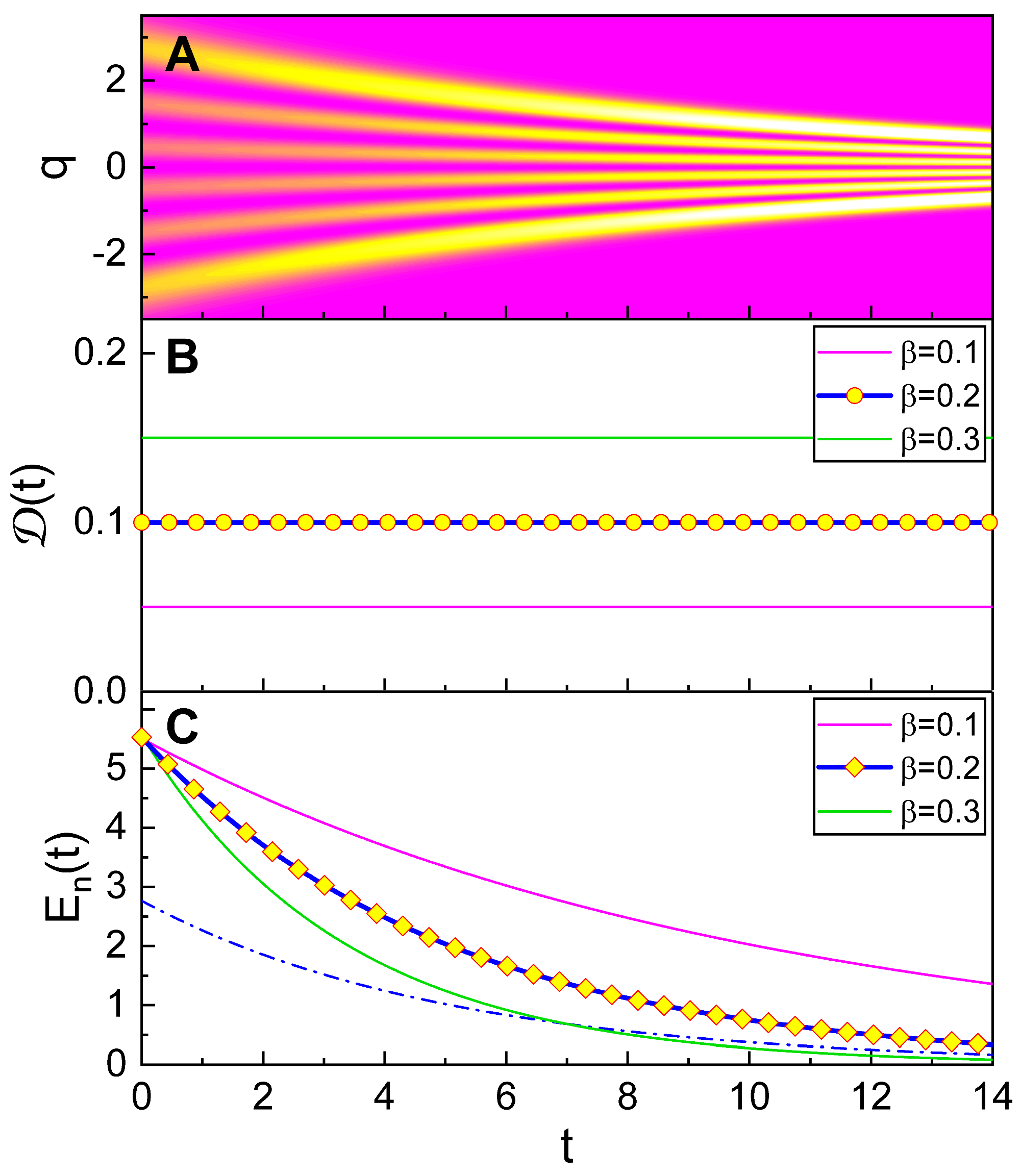
The wave functions and the quantum energies of this quantum light are represented in Methods Section 4.2. We can easily confirm from the formula of the corresponding wave functions given in Equation (24) that and , where . Hence the ratio defined in the previous subsubsection is a positive constant in this case. The temporal evolution of the wave function (with ), the ratio , and the quantum energy have been illustrated in Figure 1. Because is positive and does not depend on time, its RMS value, i.e., the measure of nonstaticity is the same as , and it is given by
This is large when is great. Hence, the nonstatic property is prominent when the waves are highly dissipative. In the limit of the nondissipative light (), the measure of nonstaticity reduces to zero: .
The width of the probability density which is illustrated in Figure 1A decreases by degrees as time goes by. Hence, an important consequence which we would like to point out is that the wave function contracts through the lapse of time when is positive. Of course, the contraction of the wave function is accompanied by gradual dissipation of the quantum energy and its components, electric and magnetic energies, as can be seen from Figure 1C. When is high, such dissipations are also large (see green curves in Figure 1B,C).
As well as the consideration of the quadrature q, its conjugate quadrature p is of key importance in the interpretation of the nonstatic waves. Regarding this, let us see the Wigner distribution functions which are defined in this case as
By using Equation (24), we readily have [26]
where are the Laguerre polynomials and
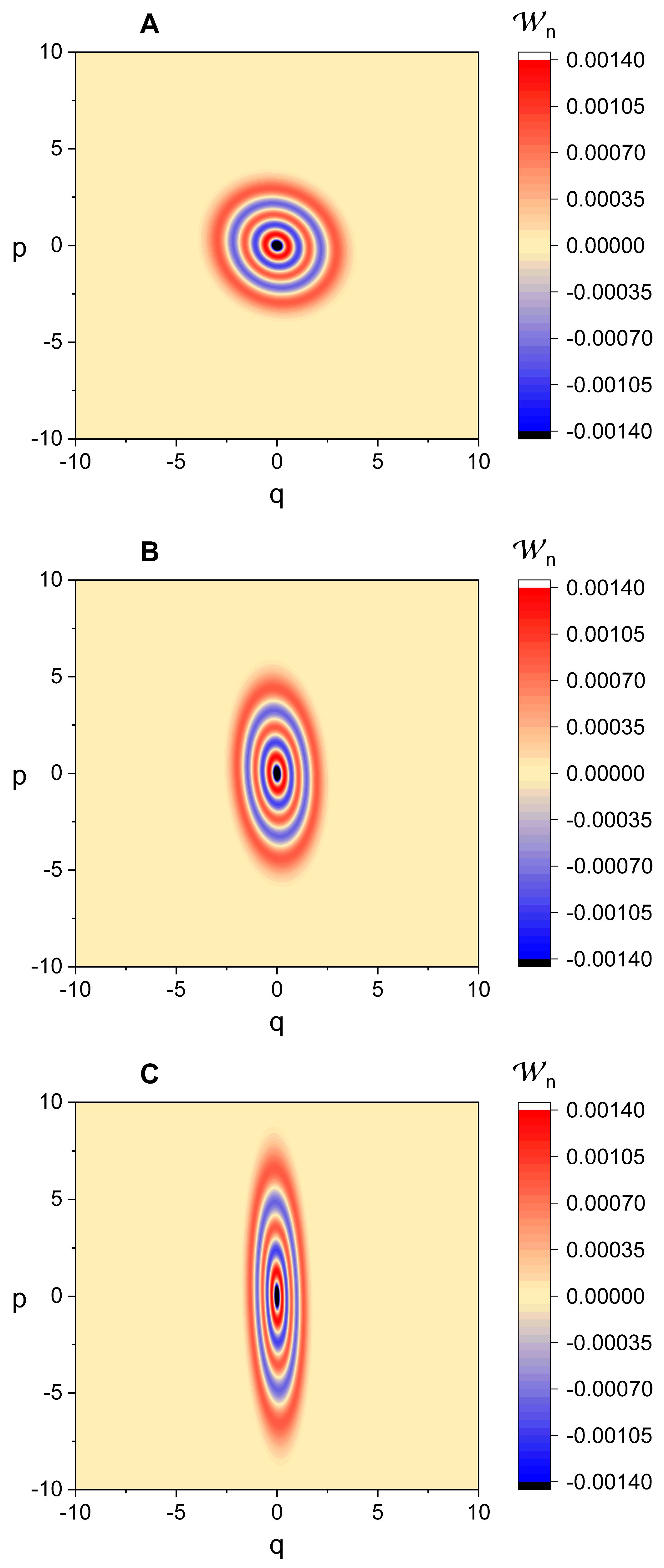
The function in Equation (6) has been illustrated in Figure 2. This figure shows that the uncertainty of q becomes small as time goes by. On the other hand, the uncertainty of p grows with time as expected by the Heisenberg limit. This outcome agrees with the analysis given in Ref. [26].
Amplifying Quantum Light Waves
Now we will see the nonstatic properties of light waves which undergo amplification. Light waves are amplified when the electric conductivity is negative [27,28,29]. The classical equation of motion for these waves is obtained by replacing from Equation (2), such that
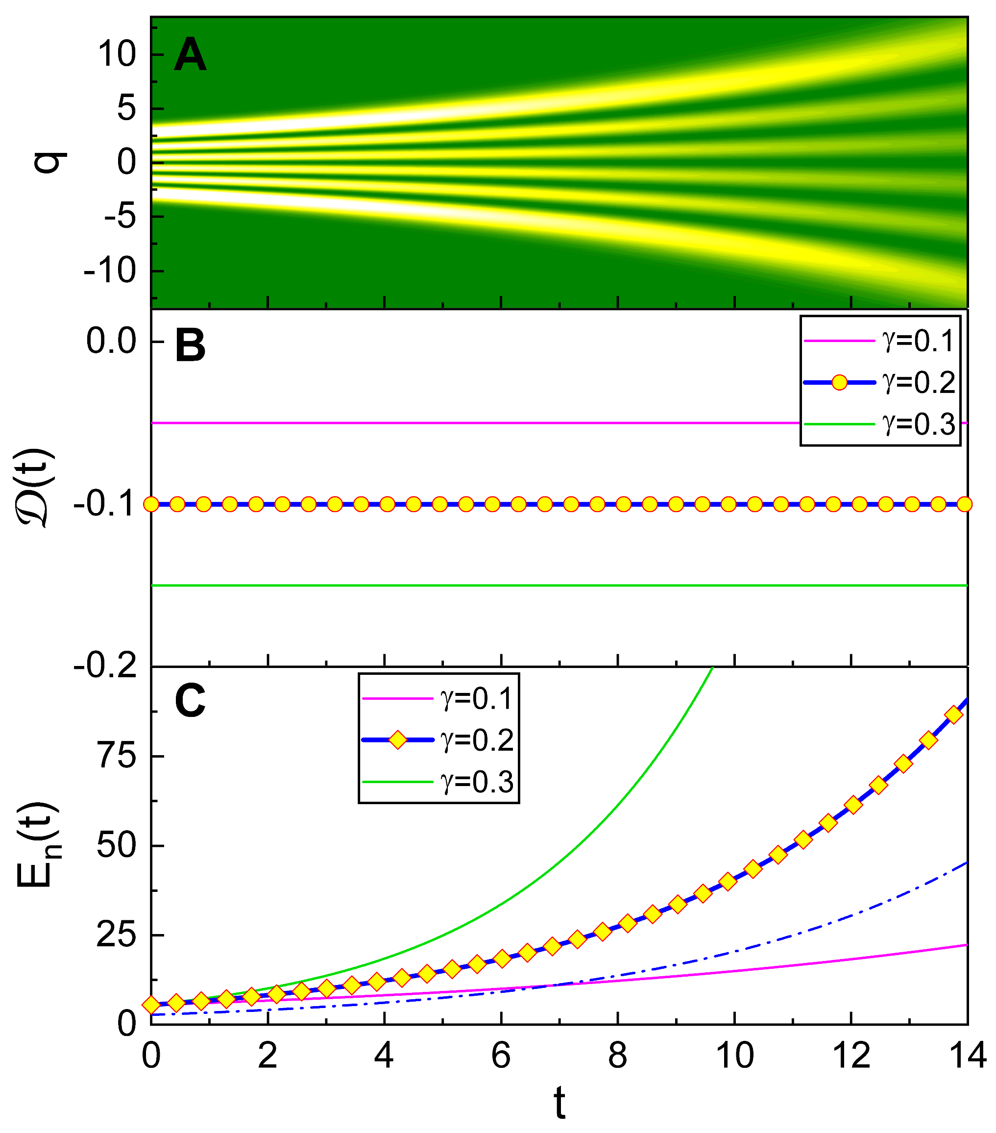
where is known as the amplification constant. The quantum wave functions in the Fock state and the corresponding quantum energies are represented in Methods Section 4.3. Because and where (see Equation (28) in Methods Section 4.3), is a negative constant in this case. The temporal behavior of the probability density associated with the wave function is shown in Figure 3, together with the corresponding behaviors of and the quantum energy. From Figure 3B, we see that is different depending on the strength of amplification. From the RMS value of , we have the associated measure of nonstaticity as
This relation shows that the nonstatic property of the waves grows as becomes large. This consequence can be compared to the fact that, for a dissipative wave, nonstatic features become prominent when is large.
From Figure 3A, we see that the probability density for this case gradually expands over time as a consequence of the wave amplification. We thus confirm that the wave function expands when is negative. This is contrast to the result of the former analysis in this subsubsection, which is that the wave function shrinks when is positive. We now emphasize these consequences and they will be used as basic tools for interpreting the characteristics of several types of more general nonstatic waves subsequently.
Figure 3C shows amplification of the corresponding quantum energy. When the measure of nonstaticity is large, the rate of the exponential growth of the energy is high.
2.2. Interpreting Periodic Nonstatic Wave Behavior
The standard wave functions for nondissipative light which is described by the simple harmonic oscillator (SHO) is static. By the way, we have shown in the previous work [12] that the quantum description of light waves in a static environment through the SHO Hamiltonian allows more generalized Schrödinger solutions related to nonstatic wave phenomena. If we regard that not only the electromagnetic parameters in the medium but the quantum energy of the wave does not vary over time in this case, such an emergence of nonstatic waves is remarkable.
The SHO Hamiltonian for such waves in quantum optics is given by
The mathematical formula of nonstatic light waves associated with this Hamiltonian have been described in Methods Section 4.4. From the wave functions given in Equation (32), we easily confirm that [12]
where
while A, B, and C are real constants which obey with , is an arbitrary phase, and is a fixed time.
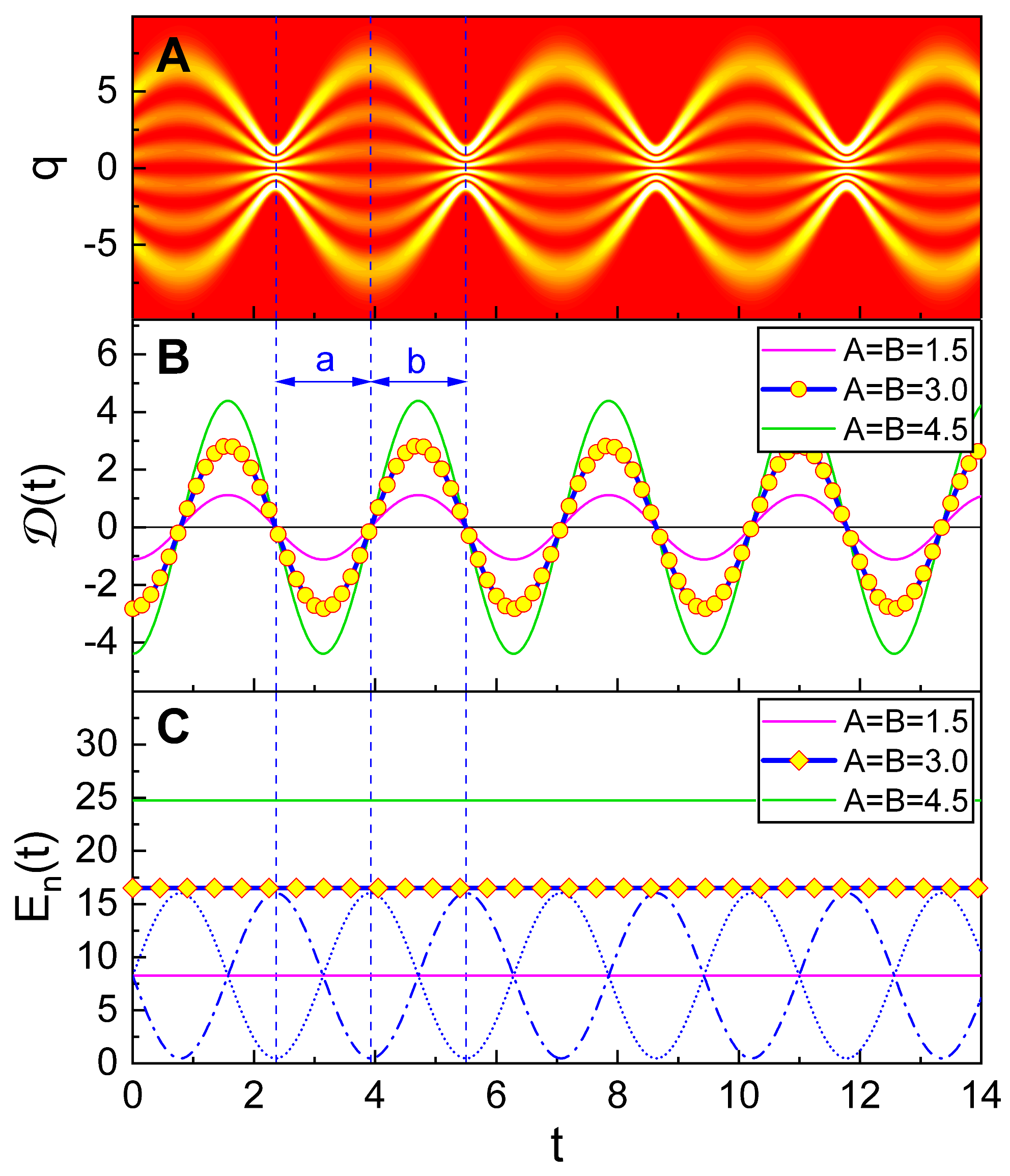
The temporal nonstatic behaviors of the probability density and relevant physical quantities for this wave have been illustrated in Figure 4. Figure 4A shows periodic collapse and expansion of the wave, while Figure 4B is the time behavior of . We see from these two figure panels that the wave collapses when is positive, whereas it expands when is negative. Notice that the mechanism of this periodic temporal behavior exactly coincides with the analyses of the previous subsection that have been carried out with the damped wave and the amplified one. Because the probability density exhibits a node in the figure whenever it is maximally collapsed and a belly whenever its expansion is largest, the wave graphic exhibits a node and a belly in turn successively. If we regard the result of the previous analysis for the dissipative wave based on the Wigner distribution function, we can confirm that a regular time-varying squeezing of the Fock state takes place along this consequence, i.e., a node accompanies the squeezing in q quadrature whereas a belly the squeezing in p quadrature.
Figure 4C is quantum energy with its electric and magnetic components, which are drawn using their exact formulae shown in Ref. [12]. Quantum electric (magnetic) energy is maximum at nodes (bellies) and minimum at bellies (nodes). However, the total optical energy does not vary over time according to the energy conservation law.
The quantitative measure of nonstaticity for this wave is given by [12]
This formula shows that the nonstatic characteristics of the wave are prominent when the values of A and B are large.
So long as the environment neither explicitly vary over time nor respond to a light wave in which propagates, the wave may be described by time-independent Hamiltonian given in Equation (10). By the way, if the intensity of a light wave in a medium is too strong, the atoms in the medium may respond nontrivially to the wave. Then, the medium is no longer static and the Hamiltonian for describing the light wave in it becomes a time-dependent one instead of Equation (10). As an example, if a medium consisting of two-level atoms is strongly driven by a resonant plane-wave, atoms which constitute the environment will emit light with the Mollow’s triplet spectrum [30]. This brings about a modification in the overall wave field in the medium. The analysis of nonstatic quantum light waves in such a situation may be worthwhile as a further research topic in the future.
It may be interesting to investigate the waves that undergo both the dissipation (or expansion) and the periodical behavior of collapse and expansion which has been managed now. These generalized nonstatic waves will be considered in the subsequent subsection.
2.3. Analysis of Generalized Nonstatic Waves
Quantum description of light waves that we have managed in the previous subsection can be generalized to the cases of more complicated light wave phenomena associated with the wave nonstaticity. As such generalization, we first consider dissipative waves of which quantum behaviors are unified with the periodical collapse and expansion. The characteristic of these waves is nontrivial and may be interesting. In this case, the classical equation of motion is the same as Equation (2) that we have already used for the analysis of the damped light waves. From the Schrödinger equation, we can extend the wave functions given in Equation (32) so that they involve the effect of dissipation, such that
where , and
with , while is a phase. This is the generalization of the damped-harmonic-oscillator description of the light waves that we have already managed. The subscript GD in Equation (15) means the Generalized Damped-harmonic-oscillator wave functions.
The ratio in this case is given by
A minor evaluation using Equation (16) results in
where
Here, is the two-variable inverse function of , where this function is defined in the range . Thus, from the RMS value of Equation (18), we have the measure of nonstaticity as
For , this reduces to , which is the same as Equation (4). On the other hand, for , this results in , which corresponds to Equation (14).
Now let us see the quantum energies of the system. For a dissipative quantum system, the energy operator is different from the Hamiltonian of the system and the relation between them can be represented in our case as [9,31,32]. Hence, the quantum electric energies and the magnetic energies are given by and , respectively, where . We can easily derive the expectation values and using the wave functions given in Equation (15). Through this, we have
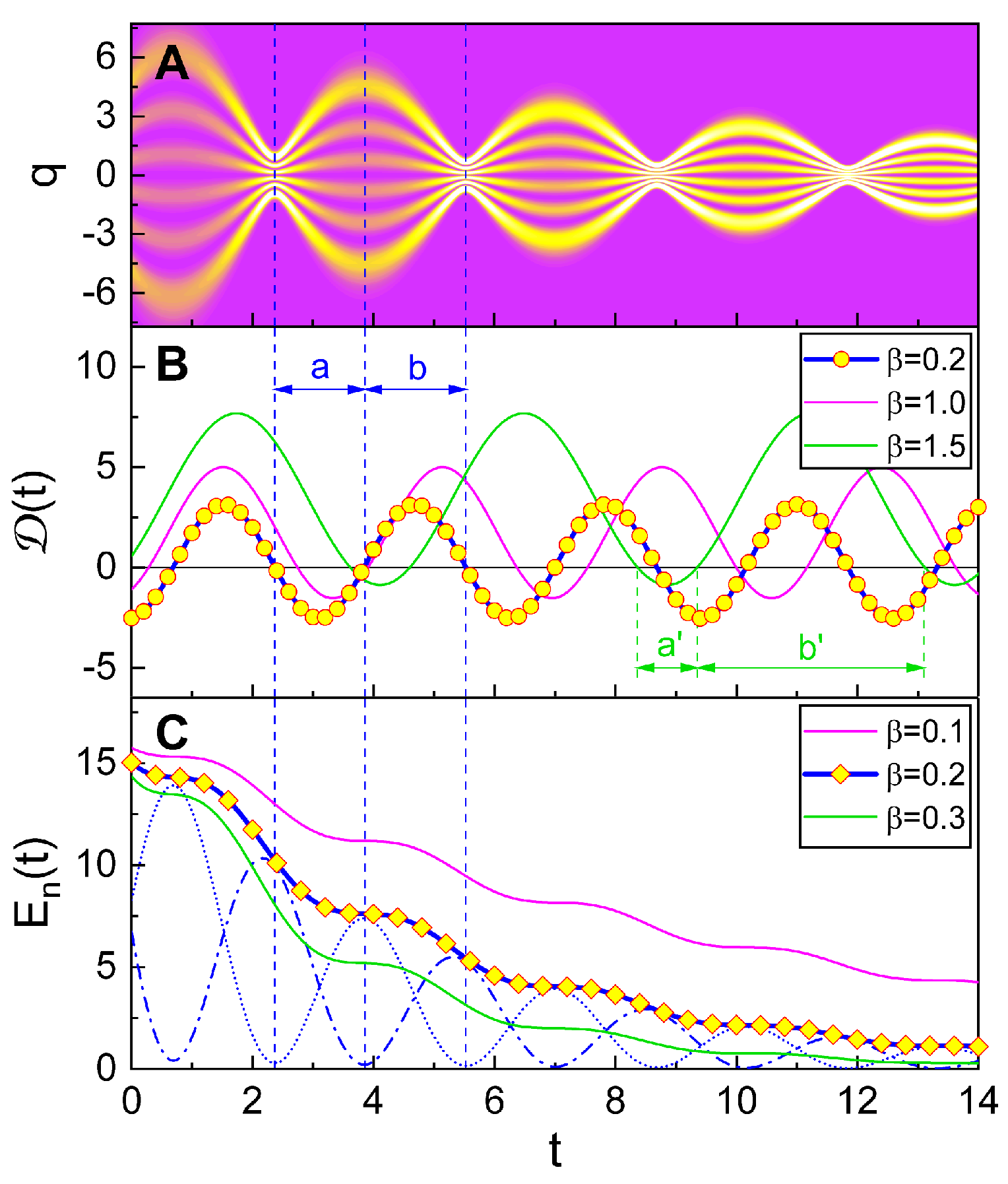
Figure 5 shows the evolution of the probability density for the corresponding nonstatic wave together with the value of and the quantum energy. We see from Figure 5A that the wave exhibits an intricate effect; it periodically changes between collapse and expansion where the amplitude of such a variation gradually dissipates as expected. When is large, the positive value of is dominant (see, especially, Figure 5B with ). This implies that the rate of dissipation grows as increases, which agrees with our intuition.
Whenever the wave has an instantaneous maximum electric energy, the differentiation of with respect to time results in zero: . Hence, from the direct time derivative of Equation (21), we can have the instants of time that the wave takes an instantaneous maximum electric energy. For instance, for the case of Figure 5C with , such instants are given by
The wave energy highly dissipates when the electric energy is large in general. You can confirm from Figure 5C that the rate of the energy dissipation is instantaneously maximum at the instants of time given above. Such instants are near the instants where the wave composes nodes, but not exactly coincide with that instants.
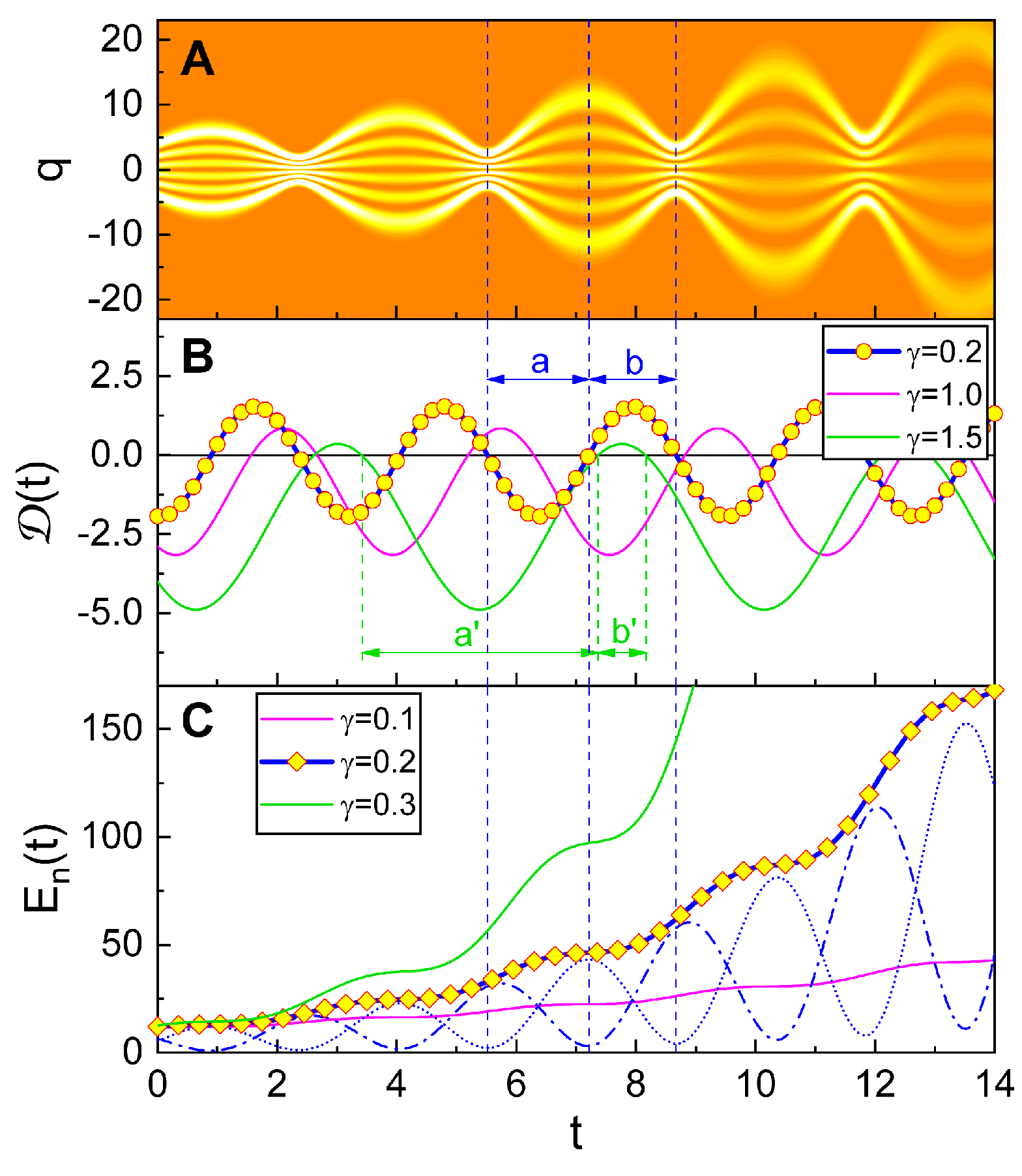
We can also investigate the quantum behavior of the nonstatic light waves which periodically collapse and expand where the amplitudes of such variations are gradually amplified. In this case, the wave functions, , can be easily obtained by replacing and from Equation (15) with Equation (16) (The subscript GA means the Generalized Amplified-harmonic-oscillator wave functions). All other outcomes corresponding to those of the lastly treated nonstatic waves can also be obtained by the same replacements from the subsequent equations, Equations (17)–(22).
The time evolution of the probability density with and for this wave has been depicted in Figure 6. We see that the envelope of the probability density gradually expands with time. Figure 6B shows that negative value of is dominant through the considered time in the graphic than the positive, especially when is large (in particular, see the case of ). Hence, the wave amplification becomes prominent as grows. The quantum energy also increases highly when is great (see Figure 6C). The rate of the energy increase is instantaneously largest whenever the wave attains an instantaneous maximum electric energy.
3. Conclusions
We have investigated the properties of nonstatic quantum light waves. The wave functions for such waves are described in terms of the complex time function . Although nonstatic characteristics do not appear in light waves when is real (), its imaginary part always appears when the waves exhibit nonstatic properties. Hence, the nonzero value of is responsible for the emergence of nonstatic characters in the waves. More clearly speaking, the temporal nonstatic behavior of the waves is determined by which is the ratio .
For the damped light waves described in the usual manner, is positive and the wave functions gradually shrink towards the origin of the quadrature q over time, while the corresponding energies dissipate in the same situation. On the other hand, is negative for the waves that exhibit amplification. From these, we can deduce a simple universal consequence that the wave functions for a quantum light undergo contraction when is positive, whereas they are amplified when is negative. Alternatively speaking, the behavior of the nonstatic wave is governed by the quadratic exponent of the exponential function which appears in the wave eigenfunction; because is always positive for a wave confined in a finite region, the wave expands when the imaginary part of the coefficient of the quadratic exponent is positive, whereas the wave collapses when the imaginary part negative. The illustration of this outcome and its applications in elucidating the characteristics of general nonstatic quantum waves were the main subject of this work.
We have used the rule for wave contraction and expansion that has been mentioned above in interpreting the specific property of nonstaticity of the waves described by the SHO Hamiltonian. According to periodical change of for these waves, the corresponding wave functions collapse when is positive while they stretch when is negative. Along this consequence, the maximally collapsed waves constitute a node in the wave graphic, whereas a belly takes place when the extension of the waves is highest. This is the reason the waves exhibit an interesting time behavior which is that they form a node and a belly in turn successively.
We have applied this periodical wave evolution in describing a generalized quantum behavior of the damped nonstatic light waves. Although the waves, in this case, exhibit a periodical behavior which is that they form nodes and bellies, the envelope of the waves shrinks by degrees according to the dissipation of the quantum wave energy. Such a gradual contraction in envelope was explained from the dominance of the positive value of than the negative through the given time in the graphic. The rate of dissipation of the quantum energy is instantaneously greatest whenever its electric component reaches a maximum value.
We have also investigated the quantum nonstatic characteristics of the waves which exhibit periodical collapse and expansion, where the wave envelope is amplifying as time goes by. We have confirmed that negative value of is dominant over time than positive in this case. The rate of the quantum-energy amplification is instantaneously largest whenever the wave attains an instantaneous greatest electric energy.
4. Methods
4.1. Methods Summary
The wave functions of the nonstatic light waves are described in terms of , where is a complex time function. If we define where and are real and imaginary parts of , respectively, the time behavior of the nonstatic light waves is governed by the value of . When is positive, the wave functions gradually shrink over time, whereas they expand when is negative. For the case of the nonstatic quantum light waves described by the simple harmonic oscillator, they collapse and expand in turn depending on the periodical change of the sign of . We can also conveniently use the variation of the sign of for analyzing more complicated nonstatic time behaviors of light waves illustrated in Figure 5 and Figure 6.
4.2. Standard Quantum Description of the Damped Waves
We briefly survey the quantum characteristics of the damped waves that have been described in Refs. [31,32,33,34,35]. If we assume underdamping in this case, the wave functions are of the form [32,33,34]
where is defined in the text, and
The subscript D in the left-hand side of Equation (24) means the Damped-harmonic-oscillator wave functions. If we take the limit , Equation (24) reduces to the familiar standard wave functions, , of the quantum light described by the SHO Hamiltonian (The subscript S means the Simple-harmonic-oscillator wave functions). Quantum electric energies and the magnetic energies of the system are given by [9]
Because and are equal each other, the quantum energies are twice of (or ) [32]:
We confirm that these exponentially decay as time goes by.
4.3. Standard Quantum Waves That Undergo Amplification
The waves that exhibit amplification can be described by replacing from the description of the damped waves, where is the amplification constant. Thus, from such a replacement from Equation (24), we have the wave functions of the amplification waves as [32]
where is defined in the text, and
The subscript A in left-hand side of Equation (28) means the Amplified-harmonic-oscillator wave functions.
The corresponding quantum electric energies, the magnetic energies, and the total quantum energies are given by [32]
Hence, the quantum energies undergo exponential increase in this case.
4.4. Quantum Waves That Exhibit Periodical Collapse and Expansion
The wave functions for a nonstatic wave that is described by the SHO Hamiltonian given in Equation (10) are represented as [12]
where is given in Equation (12) in the text, and . These are the generalization of the well-known standard wave functions, , of the quantum light that is described by SHO. The subscript GS in Equation (32) means the Generalized Simple-harmonic-oscillator wave functions. The probability densities associated with these waves exhibit periodical collapse and expansion with time (see Figure 4A). If we take the limit and from given in Equation (12), the wave functions in Equation (32) reduce to .
Funding
This research received no external funding.
Institutional Review Board Statement
Not applicable.
Informed Consent Statement
Not applicable.
Data Availability Statement
Not applicable.
Conflicts of Interest
The author declares no conflict of interest.
Abbreviations
The following abbreviations are used in this manuscript:
| RMS | Root-Mean-Square |
| SHO | Simple Harmonic Oscillator |
| S (subscript) | Simple-harmonic-oscillator wave functions () measure of nonstaticity for Simple-harmonic-oscillator wave functions () |
| D (subscript) | Damped-harmonic-oscillator wave functions () modified angular frequency of the Damped harmonic oscillator () measure of nonstaticity for Damped-harmonic-oscillator wave functions () |
| A (subscript) | Amplified-harmonic-oscillator wave functions () modified angular frequency of the Amplified harmonic oscillator () measure of nonstaticity for Amplified-harmonic-oscillator wave functions () |
| GS (subscript) | Generalized Simple-harmonic-oscillator wave functions () measure of nonstaticity for Generalized Simple-harmonic-oscillator wave functions () |
| GD (subscript) | Generalized Damped-harmonic-oscillator wave functions () measure of nonstaticity for Generalized Damped-harmonic-oscillator wave functions () |
| GA (subscript) | Generalized Amplified-harmonic-oscillator wave functions () |
References
- Kunz, K.S. Propagation of an Electromagnetic Wave in a Time-Varying Medium, Part I, General Theory; Sandia Corporation: Albuquerque, NM, USA, 1964. [Google Scholar]
- Akhmanov, S.A.; Sukhorukov, A.P.; Chirkin, A.S. Nonstationary phenomena and space-time analogy in nonlinear optics. Sov. Phys. JETP 1969, 28, 748–757. [Google Scholar]
- Dodonov, V.V.; Klimov, A.B.; Nikonov, D.E. Quantum phenomena in nonstationary media. Phys. Rev. A 1993, 47, 4422–4429. [Google Scholar] [CrossRef] [PubMed]
- Shvartsburg, A.B. Optics of nonstationary media. Phys. Usp. 2005, 48, 797–823. [Google Scholar] [CrossRef]
- Trofimov, V.A.; Lysak, T.M.; Loginova, M.M. Laser pulse self-similar propagation in a medium with noble metal nanoparticles under conditions of non-stationary processes. In Nanoengineering: Fabrication, Properties, Optics, and Devices XV (Vol. 10730, p. 1073014); International Society for Optics and Photonics: San Diego, CA, USA, 2018. [Google Scholar]
- Shvartsburg, A.B.; Petite, G. Instantaneous optics of ultrashort broadband pulses and rapidly varying media. Prog. Opt. 2002, 44, 143–214. [Google Scholar]
- Shah, S.M.; Samar, R.; Raja, M.A.Z. Fractional-order algorithms for tracking Rayleigh fading channels. Nonlinear Dyn. 2018, 92, 1243–1259. [Google Scholar] [CrossRef]
- Wu, J. Riemann-Hilbert approach of the Newell-type long-wave–short-wave equation via the temporal-part spectral analysis. Nonlinear Dyn. 2019, 98, 749–760. [Google Scholar] [CrossRef]
- Choi, J.R. The decay properties of a single-photon in linear media. Chin. J. Phys. 2003, 41, 257–266. [Google Scholar]
- Habibi, M.; Ghamari, F. Investigation of non-stationary self-focusing of intense laser pulse in cold quantum plasma using ramp density profile. Phys. Plasmas 2012, 19, 113109. [Google Scholar] [CrossRef]
- Zhaqilao. Nonlinear dynamics of higher-order rogue waves in a novel complex nonlinear wave equation. Nonlinear Dyn. 2020, 99, 2945–2960. [Google Scholar] [CrossRef]
- Choi, J.R. On the possible emergence of nonstatic quantum waves in a static environment. Nonlinear Dyn. 2021, 103, 2783–2792. [Google Scholar] [CrossRef]
- Xu, G.; Vocke, D.; Faccio, D.; Garnier, J.; Roger, T.; Trillo, S.; Picozzi, A. From coherent shocklets to giant collective incoherent shock waves in nonlocal turbulent flows. Nat. Commun. 2015, 6, 8131. [Google Scholar] [CrossRef] [Green Version]
- Wolff, C.; Stiller, B.; Eggleton, B.J.; Steel, M.J.; Poulton, C.G. Cascaded forward Brillouin scattering to all Stokes orders. New J. Phys. 2017, 19, 023021. [Google Scholar] [CrossRef] [Green Version]
- Keller, O. Quantum Theory of Near-Field Electrodynamics; Part of the Nano-Optics and Nanophotonics Book Series; Springer: Berlin/Heidelberg, Germany, 2011. [Google Scholar]
- Girard, C. Near fields in nanostructures. Rep. Prog. Phys. 2005, 68, 1883–1933. [Google Scholar] [CrossRef]
- Gong, T.; Corrado, M.R.; Mahbub, A.R.; Shelden, C.; Munday, J.N. Recent progress in engineering the Casimir effect–Applications to nanophotonics, nanomechanics, and chemistry. Nanophotonics 2021, 10, 523–536. [Google Scholar] [CrossRef]
- Kukhlevsky, S.V. Propagation of X-ray femtosecond pulses through tapered nanometer-scale capillary waveguides. Phys. Lett. A 2001, 291, 459–464. [Google Scholar] [CrossRef]
- Moody, G.; McDonald, C.; Feldman, A.; Harvey, T.; Mirin, R.P.; Silverman, K.L. Quadrature demodulation of a quantum dot optical response to faint light fields. Optica 2016, 3, 1397–1403. [Google Scholar] [CrossRef] [PubMed] [Green Version]
- Notomi, M.; Mitsugi, S. Wavelength conversion via dynamic refractive index tuning of a cavity. Phys. Rev. A 2006, 73, 051803(R). [Google Scholar] [CrossRef]
- Lähteenmäki, P.; Paraoanu, G.S.; Hassel, J.; Hakonen, P.J. Dynamical Casimir effect in a Josephson metamaterial. Proc. Natl. Acad. Sci. USA 2013, 110, 4234–4238. [Google Scholar] [CrossRef] [Green Version]
- Braunstein, S.L.; van Loock, P. Quantum information with continuous variables. Rev. Mod. Phys. 2005, 77, 513–575. [Google Scholar] [CrossRef] [Green Version]
- Louisell, W.H. Quantum Statistical Properties of Radiation; John Wiley and Sons: New York, NY, USA, 1973; p. 240. [Google Scholar]
- Caldirola, P. Forze non conservative nella meccanica quantistica. Il Nuovo Cimento 1941, 18, 393–400. [Google Scholar] [CrossRef]
- Kanai, E. On the quantization of the dissipative systems. Prog. Theor. Phys. 1950, 3, 440–442. [Google Scholar] [CrossRef]
- Wang, S.; Yuan, H.-C.; Fan, H.-Y. Fresnel operator, squeezed state and Wigner function for Caldirola-Kanai Hamiltonian. Mod. Phys. Lett. A 2011, 26, 1433–1442. [Google Scholar] [CrossRef] [Green Version]
- Ryzhii, V.; Satou, A. Electric-field breakdown of absolute negative conductivity and supersonic streams in two-dimensional electron systems with zero resistance/conductance states. J. Phys. Soc. Jpn. 2003, 72, 2718–2721. [Google Scholar] [CrossRef] [Green Version]
- Ryzhii, V.I. Microwave-induced negative conductivity and zero-resistance states in two-dimensional electronic systems: History and current status. Phys. -Usp. 2005, 48, 191–197. [Google Scholar] [CrossRef]
- Dorozhkin, S.I.; Dmitriev, I.A.; Mirlin, A.D. Negative conductivity and anomalous screening in two-dimensional electron systems subjected to microwave radiation. Phys. Rev. B 2011, 84, 125448. [Google Scholar] [CrossRef] [Green Version]
- Mollow, B.R. Power spectrum of light scattered by two-level systems. Phys. Rev. 1969, 188, 1969–1975. [Google Scholar] [CrossRef]
- Um, C.-I.; Yeon, K.-H.; George, T.F. The quantum damped harmonic oscillator. Phys. Rep. 2002, 362, 63–192. [Google Scholar] [CrossRef]
- Choi, J.R.; Zhang, S. Quantum and classical correspondence of damped-amplified oscillators. Phys. Scr. 2002, 66, 337–341. [Google Scholar] [CrossRef]
- Baldiotti, M.C.; Fresneda, R.; Gitman, D.M. Quantization of the damped harmonic oscillator revisited. Phys. Lett. A 2011, 375, 1630–1636. [Google Scholar] [CrossRef] [Green Version]
- Choi, J.R. Emergence of classicality from initial quantum world for dissipative optical waves. Adv. Electromagn. 2016, 5, 25–31. [Google Scholar] [CrossRef] [Green Version]
- Yeon, K.-H.; Kim, S.-S.; Moon, Y.-M.; Hong, S.-K.; Um, C.-I.; George, T.F. The quantum under-, critical- and over-damped driven harmonic oscillators. J. Phys. A Math. Gen. 2001, 34, 7719–7732. [Google Scholar] [CrossRef]
Figure 1.
Contour plot of the probability density (A) as a function of q and t for the quantum wave given in Equation (24), where we have chosen ; the corresponding temporal evolutions of the ratio (B) and the quantum energy (C) for several different values of . The extra line in (C), i.e., the dash-dot line is quantum electric energy for the case of , whose value is in fact the same as the magnetic energy . We have used , , , and . For convenience, we take all values being dimensionless for this and subsequent figures. This figure illustrates gradual wave collapse.

Figure 2.
Contour plot of [Equation (6)] for several different times: we have chosen for (A), for (B), and for (C). We used , , , , and : these choices correspond to the wave in Figure 1A.

Figure 3.
Contour plot of the probability density (A) as a function of q and t for the quantum wave given in Equation (28), where we have chosen ; the corresponding temporal evolutions of the ratio (B) and the quantum energy (C) for several different values of . The extra line (the dash-dot line) in C is quantum electric energy () for the case of . We have used , , , and . This figure shows amplification of the quantum light wave.

Figure 4.
Contour plot of the probability density (A) as a function of q and t for the quantum wave given in Equation (32), where we have chosen ; the corresponding temporal evolutions of the ratio (B) and the quantum energy (C) for several different values of A and B. a and b in (B) are examples of time intervals of wave expansion and collapse, respectively. The extra curves in (C), i.e., the dash-dot curve and the dotted curve are quantum electric energy and the magnetic energy , respectively, for the case of . Whereas the taken values of A and B are designated in the legends, C is taken to be : this convention will also be used throughout the subsequent figures. We have used , , , , , and . We see from this figure that successive changes of the sign of induce periodical wave collapse and amplification.

Figure 5.
Contour plot of the probability density (A) as a function of q and t for the quantum wave given in Equation (15), where we have chosen ; the corresponding temporal evolutions of the ratio (B) and the quantum energy (C) for several different values of . a and b ( and ) in (B) are examples of time intervals of wave expansion and collapse, respectively, for (). The extra curves in (C), i.e., the dash-dot curve and the dotted curve are quantum electric energy and the magnetic energy , respectively, for the case of . We have used , , , , , , and . This figure shows novel features of the general nonstatic waves, i.e., periodical behavior of wave collapse and expansion combined with the gradual dissipation.

Figure 6.
Contour plot of the probability density (A) as a function of q and t, where we have chosen ; the corresponding temporal evolutions of the ratio (B) and the quantum energy (C) for several different values of . a and b ( and ) in (B) are examples of time intervals of wave expansion and collapse, respectively, for (). The extra curves in (C), i.e., the dash-dot curve and the dotted curve are quantum electric energy and the magnetic energy , respectively, for the case of . We have used , , , , , , and . This figure corresponds to complicated general nonstatic waves which exhibit periodical wave collapse and expansion unified with the gradual expansion.

Publisher’s Note: MDPI stays neutral with regard to jurisdictional claims in published maps and institutional affiliations. |
© 2021 by the author. Licensee MDPI, Basel, Switzerland. This article is an open access article distributed under the terms and conditions of the Creative Commons Attribution (CC BY) license (https://creativecommons.org/licenses/by/4.0/).
Share and Cite
MDPI and ACS Style
Choi, J.R. Characteristics of Nonstatic Quantum Light Waves: The Principle for Wave Expansion and Collapse. Photonics 2021, 8, 158. https://0-doi-org.brum.beds.ac.uk/10.3390/photonics8050158
AMA Style
Choi JR. Characteristics of Nonstatic Quantum Light Waves: The Principle for Wave Expansion and Collapse. Photonics. 2021; 8(5):158. https://0-doi-org.brum.beds.ac.uk/10.3390/photonics8050158
Chicago/Turabian StyleChoi, Jeong Ryeol. 2021. "Characteristics of Nonstatic Quantum Light Waves: The Principle for Wave Expansion and Collapse" Photonics 8, no. 5: 158. https://0-doi-org.brum.beds.ac.uk/10.3390/photonics8050158
Note that from the first issue of 2016, this journal uses article numbers instead of page numbers. See further details here.