Machine Learning Methods for Quality Prediction in Production


Department of Industrial and Manufacturing Systems Engineering, Iowa State University, Ames, IA 50011, USA
*
Author to whom correspondence should be addressed.
Logistics 2020, 4(4), 35; https://0-doi-org.brum.beds.ac.uk/10.3390/logistics4040035
Submission received: 9 October 2020
/
Revised: 11 December 2020
/
Accepted: 14 December 2020
/
Published: 21 December 2020
Abstract
:The rising popularity of smart factories and Industry 4.0 has made it possible to collect large amounts of data from production stages. Thus, supervised machine learning methods such as classification can viably predict product compliance quality using manufacturing data collected during production. Elimination of uncertainty via accurate prediction provides significant benefits at any stage in a supply chain. Thus, early knowledge of product batch quality can save costs associated with recalls, packaging, and transportation. While there has been thorough research on predicting the quality of specific manufacturing processes, the adoption of classification methods to predict the overall compliance of production batches has not been extensively investigated. This paper aims to design machine learning based classification methods for quality compliance and validate the models via case study of a multi-model appliance production line. The proposed classification model could achieve an accuracy of 0.99 and Cohen’s Kappa of 0.91 for the compliance quality of unit batches. Thus, the proposed method would enable implementation of a predictive model for compliance quality. The case study also highlights the importance of feature construction and dataset knowledge in training classification models.
1. Introduction
Production and operational efficiency are essential for the competitiveness of manufacturing companies, especially effective quality control. Reworks, reverse logistics, and production plan disruptions due to defective products are some of the problems caused for an organization’s logistics by lack of quality. In the recent decades, modern manufacturing quality departments have shifted their focus from reactive to proactive methods. There has been significant progress in defect prevention via process improvements. However, as the requirement for quality increases, the cost of preventing defects could start to outweigh potential savings [1]. Current quality control strategies in manufacturing focus on continuous improvement to identify root causes of defects and implementing preventive measures. However, defects such as a mislabeled product, or a product assembled with missing parts have significantly greater penalties for escaping as compared to the costs incurred correcting such defects. In such situations, using a prediction model to preemptively contain and rework batches of defective product could provide greater return on investment as compared to efforts aimed at eliminating the causes of the defect. Currently used qualitative methods such as root cause analysis require significant involvement from skilled personnel to subjectively evaluate the effects of various causes. Thus, there is potential for root cause analysis to be supplemented with insight on factors that attribute to the defects by examination of the predictive model.
Presently, research has successfully demonstrated the use of machine learning techniques to predict the effects of process parameters in various manufacturing operations [2]. However, there have been relatively fewer applications that aim to predict the compliance quality of finished goods from data pertaining to a sequence of operations, on a production line. The research by Kerdprasop et al. could predict quality defects from multistage semiconductor manufacturing with Cohen’s Kappa of 0.57 [3], while the work by Kao et al. and Arif et al. in the same context could predict defects with Cohen’s Kappa of 0.98 [4] and 0.04 [5], respectively. However, these papers did not use classification algorithms like neural networks or bagged and boosted ensembles. Furthermore, the datasets used for training and evaluation were relatively balanced in class distribution, thus not needing the methods to address class imbalance. Defect rates in modern manufacturing tend to be low, resulting in datasets where the predicted class has significant imbalance. This paper aims to address these areas of improvement in the current research by addressing various practical issues arising from the use of machine learning in multistage manufacturing and training prediction models with comparable performance.
Data mining is the practice of using data to discover patterns and relations between attributes. With the abundance of modern manufacturing and process data, it has become feasible for the application of data mining in various use-cases such as inductively discovering factors that affect the quality of a product [6] or effectiveness of digital marketing [7]. Data mining methods can reveal information that may often be overlooked with a hypothesis-driven approach, such as the use of statistics. There are a number of data mining and knowledge discovery techniques such as clustering and association rule mining. Clustering analysis is typically adopted for preprocessing and analysis of large datasets to find clusters of similar datapoints [8]. Association rule mining is used to discover interesting relations between attributes in a dataset [9]. Both of these techniques do not have a clearly defined response attribute. Machine learning shares similarities with data mining such as being a subset of artificial intelligence, but it differs in its objective. Machine learning is used to aid in the completion of specific tasks rather than extract knowledge from data [10]. Classification is an example of machine learning since its methods are used to create classification models which are used for the prediction of discrete response variables [11]. Predicting the compliance quality of incoming parts from a manufacturing line is the problem addressed in this paper and it is an example of the use-case for classification in manufacturing industries [12].
Modern classification methods such as the ensemble models benefit from improvements in the computing capacity of modern systems [13], supporting the widespread use of machine learning methods. This is because the frequently used ensemble classifiers such as random forest and adaptive boosting often combine weak learners like simple decision trees, Naive Bayes, and k-nearest neighbor into an ensemble to combine the strengths of individual learners. Another challenge often faced in real applications is the classification of imbalanced datasets [14]. This is because most classification algorithms tend to learn models that are biased in favor of the majority class. Compliance quality in manufacturing plants is a good example of class imbalance since defective product units are in the heavy minority as compared to compliant units [15]. This study aims to shed some light on classification for imbalanced datasets since the focal problem is the classification of manufacturing quality non-compliance. Special attention has been devoted in the method design to address the imbalanced nature of such datasets.
Imbalanced classification has become an increasingly prominent obstacle in practical settings such as credit card fraud detection [16], fault detection in machinery [17], and diagnosis of cerebrovascular disease [18]. In these applications, the importance of correctly classifying the minority outweighs that of the majority class. When a dataset has a significant imbalance, it poses a challenge for classification of the minority class since a prediction model tends to favor correctly classifying the majority class. Lack of data points of the minority class makes it challenging to train an accurate model [14]. Current research has yielded solutions in the forms of feature engineering and learning algorithm-based approaches to improve the accuracy of minority class prediction [18].
Feature engineering methods to address imbalance datasets include the general sampling techniques and methods that are dataset specific such as high-level feature construction and selection [19]. Sampling methods focus on reducing the class imbalance by oversampling the minority, under sampling the majority class, or generating new data points of the minority class from existing data points via SMOTE [20]. However, the use of random under sampling results in loss of information regarding the majority class whereas random oversampling can result in overfitting the model to training data. SMOTE attempts to reduce overfitting by generating new data points via interpolation of nearest neighbor minority class. Improving the performance of classifiers for the minority class have yielded methods such as cost-sensitive boosting [21] and other ensemble methods that incorporate sampling within their training loops [22,23].
However, the above-mentioned methods to address imbalance do not resolve issues wherein the available features cannot be used to train an acceptable model, regardless of the currently available classification algorithms. Similar conditions can be encountered when attempting to predict the compliance quality of finished product from process data on an assembly line. Data pertaining to the manufacturing processes varies significantly in different factories and requires feature engineering before it can be used to train a classification model. An example of such feature engineering is the construction of explanatory features based on a thorough understanding of the dataset and its relevant subject matter [24]. Thus, feature construction based on dataset knowledge can provide substantially improved results. This served as one of the major motivations for application of the method described in this paper and its demonstration in the case study.
The knowledge required to construct additional features to improve classification models may require domain expertise and solutions discovered in this manner would tend to be specific for the problem addressed. This is because most practical applications of classification entail significant efforts in data consolidation, pre-processing, and understanding the use-case [18,25]. The method described in this paper pertains to quality prediction in manufacturing. As such, domain knowledge is useful when constructing features from the raw dataset and drawing conclusions from the results of training the classification models.
The rest of this paper is organized as follows. In Section 2, the proposed method for predicting manufacturing quality compliance is presented. Descriptions have been detailed for the classification methods, explanation of common features for manufacturing quality prediction and evaluation method for model performance comparison. Section 3 focuses on describing a case study to establish the context in which the proposed method is applied and the problems that it will address. Section 4 presents the results of this application in the case study and discusses possible improvements in the method specific to that case. The paper is concluded in Section 5 with a summary of findings and future research directions.
2. Materials and Method
Despite research pertaining to the application of machine learning methods to predict the response of specific processes such as quality in manufacturing [12] or arrival time for containerships [26], there is still unexplored potential for its use in predicting the final outcome of a chain of linked processes. Thus, the method proposed in this paper is intended for use in prediction of quality in manufacturing via classification but can be generalized for use in cases such as prediction of pass-or-fail compliance quality for multi-stage operations. A large dataset containing previous manufactured units with features corresponding to factors describing the unit or process parameters is required to train the model. Datasets with more features will result in a better classification model obtained via this method.
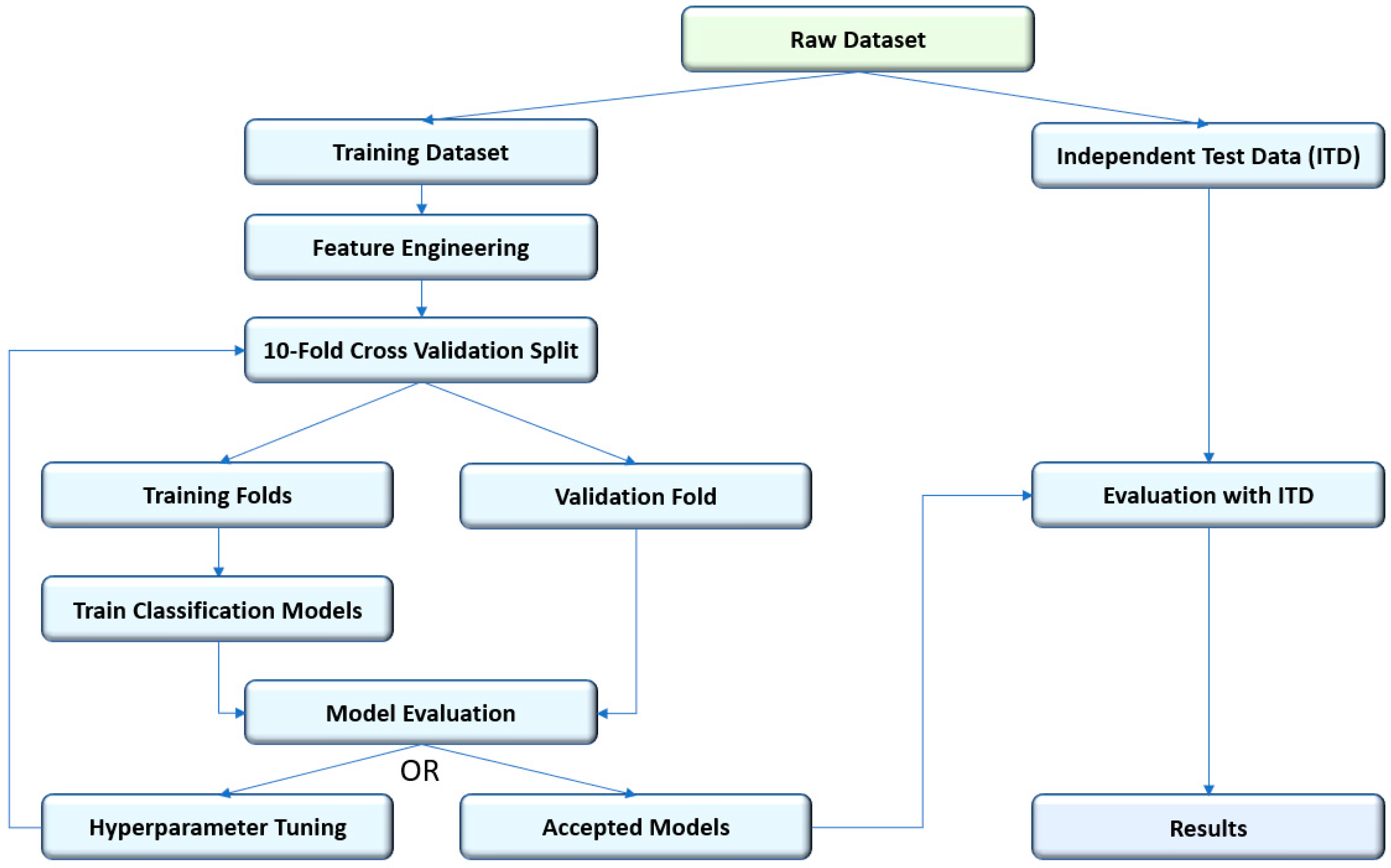
Figure 1 provides an overview of the method proposed for addressing the problem described in this paper. This method used established best practices in order to satisfactorily train and evaluate a classification model for its specialized application in the prediction of manufacturing compliance quality. Thus, applying domain knowledge when constructing features, selecting classification algorithms, or tuning hyperparameters results in superior model performance. As a first step, the data were split into training and independent test sets for evaluation. Despite the problem that would arise from sampling variance, it was beneficial to prevent overfitting the model on the training data and obtain an unbiased estimate of how the model would perform in its capacity [27] to predict manufacturing quality non-compliance. Feature selection and construction was then performed on the training dataset. Tenfold Cross Validation was then used to evaluate multiple models trained from the training dataset and tune hyperparameters of the training algorithms. While it would be beneficial to use Leave-one-out Cross Validation when tuning the hyperparameters of the classification model, it would be too computationally intensive given the number of data points available [28]. Using metrics explained later in this section, the trained models were then evaluated with the independent test dataset.
2.1. Classification Methods
Classification is used to predict the response of a discreet variable by considering its relations with other variables in the dataset [11]. Since the pass-or-fail compliance determined during final inspection in manufacturing is a discreet variable, classification methods can be used to predict such an outcome. There are multiple classification methods that can be used ranging from basics like decision trees, support vector machines and Naive Bayes to complex ensemble methods which can be broadly categorized into bagging or boosting. Since most methods have specific strengths and rely on assumptions about the nature of the dataset, the methods proposed in this paper were generalized enough for most cases pertaining to prediction of compliance quality in a manufacturing plant. Thus, the following classifiers could be used in combination to that effect.
2.1.1. Random Forest
This popular classification method is an improved form of bagging that utilizes decision trees as the weak learners [22,29]. The main advantage of random forest as compared to bagged ensembles is that it attempts to reduce bias by learning trees from a subset of features sampled from the dataset. The trained model can also be improved by tuning the number of features to sample, maximum decision tree depth and minimum instances per node. As such, its popularity and general effectiveness allowed for a good starting point in creating a collection of prediction models.
2.1.2. XGBoost
XGBoost is a relatively recent development in inductive learning [30]. This learner has been used extensively with agreement that it tends to be more computationally efficient and generally applicable for a wide range of dataset types, from common classification problems [31] to pattern recognition in time-dependent features [32].
This algorithm builds upon the gradient boosting algorithm by introducing a regularization parameter, which reduces the individual regression tree’s sensitivity towards outliers in the dataset. As such, this algorithm will result in a model that has less variance than that learned from gradient boosting alone. The use of this learner in combination with random forest provided two models that were learned from the principles of boosted and bagged ensembles of decision trees, respectively. Additional methods such as support vector machines [33] using various kernels or artificial neural networks [34] can also be used for comparison if the results of these learners do not prove satisfactory.
2.2. Feature Engineering
Raw data collected from various sources can rarely be used directly to train a classification model. Thus, feature engineering refers to the steps taken to prepare a dataset for classification. This entailed cleaning the dataset to ensure consistency of data type in each feature and removal of redundant variables. Additionally, features could be constructed to support the algorithm used to train classification models in order to obtain improved results. This was achieved by transforming and combining features in the available data to obtain new variables. In the context of manufacturing quality on a mixed-model assembly line, the following features could be derived from available production data and provide a basis for the classification model to be built from.
2.2.1. Suspicious Unit Batches
Since quality defects tend to be relatively rare in modern manufacturing and the prevalence of random inspection, only using identified defective units as a class variable will result in a poor prediction model. Thus, a new class variable accounting for random inspection for prediction was derived instead. This variable was constructed from raw data pertaining to quality defects found during unit inspection, and production line data containing serial numbers of units in the sequential order at which they flowed through production and inspection. Defining the size of a suspicious batch of units based on identified defects required consideration for the nature of randomness in inspection and desired confidence in product compliance quality.
If a factory uses production lines to manufacture goods, the progress of work-in-progress (WIP) through its production stages can be traced more consistently than a job-shop or manufacturing cell layout. As such, if the final product inspection is random and a defective unit is found, then based on the required confidence level, a certain number of units before and after the defective unit in production sequence would have to be considered under suspicion of the same defect. Thus, it would also be a good idea to segregate and inspect the other units centered around the defective unit.
The exact number of units quarantined for such a reason could vary depending on the factory’s throughput, inspection strategy and best practices. However, if a 100% inspection strategy is used then the construction of this class variable would not be necessary since there is no need to account for random inspection.
2.2.2. Proximity to a Model Changeover
In modern multi-model production lines, model changeovers have been known to cause quality defects in the assembled products [35]. Thus, a feature constructed to represent how close a unit was to a previous model changeover in its production run can result in learning a significantly improved classification model. This variable can be presented as:
- An absolute measure (s) of the unit’s sequence number (n) relative to the last model change in the sequence numbers (n0) assigned to each unit in the daily production logs.s = n − n0,
- A continuous variable (x) that measures the relative position of the unit (s) with respect to the sequence at which the model change happened (s0) and the next such model change (s1).x = (s − s0)/(s1 − s0),
2.2.3. Model Color Change
This feature was proposed on the basis of general guidelines established when investigating recurrent quality issues under suspicion of human error. A model change is much more apparent when there are stark differences between the appearance of the two models and thus should potentially reduce the likelihood of assembly errors [36] caused by the model changeover. This feature can be derived from the model change feature discussed earlier but would only apply if there was a change in color between the two models. A possible way in which this feature could be constructed was as a binary variable (c) that describes whether the previous model in the production logs was of a different color such that c = 0, if model before changeover was of same color and c = 1 if the model before changeover was of different color.
Similarly, with knowledge of the use-case, new features corresponding to transformed production data could be derived following the same principle as that mentioned above. For example, brand, assembly complexity based on bill-of-material, general appearance, or packaging methods could also be used to construct new features. Many of the features discussed earlier are generalized starting points based on best practices when troubleshooting for quality defects. Thus, expertise in the subject matter of the manufacturing processes and factors contributing to compliance quality will result in constructed features that can be used to train better classification models.
2.3. Evaluation Method
Choosing correct metrics when evaluating the performance of a classification model is crucial since each metric places varying emphasis on the overall accuracy, precision, recall, or agreement between model and ground truth for different class values. Thus, the chosen metric needs to closely evaluate model performance based on what is required from the user. In this paper, evaluation of the models was completed via Cohen’s Kappa since it is often used as a way to measure the ability of a model to predict binary classes with heavy imbalances [37].
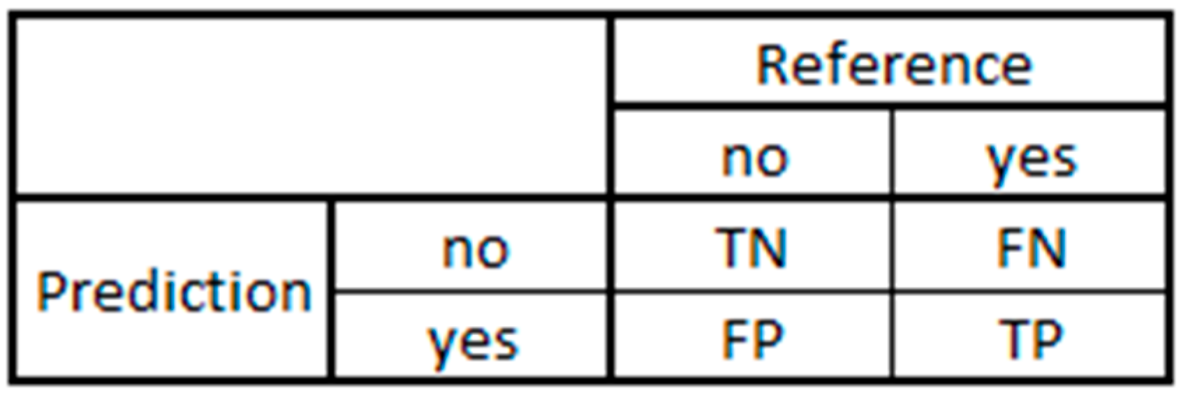
Despite the fact that a confusion matrix can comprehensively explain the performance of a model by itself, a single performance measure could make the evaluation faster. Additionally, in the context of manufacturing plants, a single metric can be easier to present in cases where cross-functional cooperation is required. Since the problem of manufacturing compliance quality being addressed in this paper can be presented as a binary class variable, the confusion matrix is much simpler, as shown in Figure 2. The class value of ‘yes’ corresponds to potentially defective units while ‘no’ represents otherwise.
Accuracy is a performance measure that can be used to evaluate classification models, using a test dataset.
It is a sum of all correct predictions divided by the total number of predictions made. This metric can be a conclusive measure of performance in most datasets where the class has attributes with mostly similar representation.
However, in cases where there is a heavy class imbalance, accuracy can be misleading as a performance measure since it does not penalize misclassification of the minority. For example, a dataset with 10% and 90% binary class distribution can allow for the high accuracy of 90% simply by allowing the classifier to predict all as the majority class. Thus, there is no guarantee with regards to the quality of the classification model, especially for the minority class when relying solely on accuracy as a performance measure.
Another popular performance measure in recent literature regarding classification is the F-measure or F1 score. It is a harmonic mean of precision and recall for the prediction of a particular value [38]. In this case, we can consider the F1 score for predicting the class attribute as ‘yes’ as shown in Figure 2.
However, a drawback of relying on the F1 measure is the fact that it does not provide a good measure of the model’s overall performance. The F1 score depends upon which value of the class variable is being considered for the evaluation [39]. In the case of Figure 2, the F1 score for class value ‘yes’ could be very different as compared to that of class value ‘no’. This would not be a problem in cases where the cost of misclassification for one value trivializes the other but in other situations, the F1 score might not be sufficient as a performance measure by itself.
As such, Cohen’s Kappa (κ) is another metric that is commonly used to evaluate the performance of classification models [37]. In the context of classification models, it is a measure of the agreement between the predictor and reference while accounting for the agreement that occurs due to chance [40].
It is a function which penalizes chanced agreement (pe) from the observed accuracy (p0).
N is the total number of observations being used to evaluate the model.
pN and pP are the probabilities of agreement between predictor and reference by chance for negative (no) and positive (yes) class values.
The advantage of using Cohen’s Kappa as opposed to F1 score was that it can summarize the performance of the model with regards to the prediction of both classes in one measure whereas the use of F1 could require evaluation for two class values. Additionally, it will account for agreement between raters due to chance. Combined with the fact that Cohen’s Kappa can be generalized for use in situations where the class can take on more than two values, it has gained popularity for use in more complex classification problems as a performance measure.
Thus, for the problem addressed in the use-case, this paper proposed the use of both Cohen’s Kappa as the singular performance metric, and the confusion matrix to consider some of the finer details about model performance regarding particular class attributes.
3. Case Study
This case study focuses on an appliance manufacturing factory that has recently undergone some major changes to one of its assembly lines. These changes include the addition of vision systems and scanners to keep track of all its produced units by their serial numbers. Additionally, there were improvements in the organization of quality assurance data regarding inspection results, returns and issue descriptions. However, there was also a rise in the number of quality defects being reported during random inspection pertaining to parts being missing or assembled wrong in the manufactured units. Despite the efforts and suggestions of various employees, it took a few months to investigate the issue and during this time, a huge amount of money had to be spent to recall units suspected to be defective back to the factory for inspection and release.
This presented an opportunity for the newly available data to be used to predict compliance quality of production runs or individual units before they even arrive at final inspection. Supervised learning could be used to train a classification model in advance. The trained model could then be used to predict the quality of units passing through a production line in real-time and contain suspected units before they escape the factory. Applications of machine learning in studies regarding quality in various manufacturing operations had yielded significant success in semiconductor manufacturing [4,41] and additive manufacturing [12].
Since most of the production lines in the factory had mixed model production with almost negligible changeover time, the entire assembly and inspection process had been streamlined to produce nearly 800 units of product daily over 3 work shifts without pause. The rushed pace of production made it difficult to recover from errors in production and thus it had become the quality engineering department’s main directive to fix and contain quality issues proactively rather than reactively.
Depending on the results of this study, a prediction model based on real-time production data could be potentially useful, as a tool to alert inspection teams to prioritize batches likely to be defective, or even as a way to learn the causes of some of the main quality issues. However, since the information systems had not undergone expansion at the time of data collection, there was a lack of detailed data available about the assembly processes. Although, if the preliminary study could deliver a feasible prediction system or useful learnings, then the general method used could be adapted to similar effect with a dataset containing more features pertaining to process and machine data.
3.1. Data Sources
The data that were used in this paper are masked quality and production data from a large-scale appliance manufacturing plant. The manufacturing dataset is structured to contain unit serials, models and production batch sequence identifiers for every unit that passes through the production line. The random customer acceptance inspection (RCAI) dataset contains the unit serial, model number, and some identifiers for the issues found. These data are then merged with the production dataset in the form of a variable that is defined by whether the unit was caught defective in the RCAI.
Table 1 describes the variables in the available merged dataset which contains 75,636 observations of eight variables, wherein the field SuspiciousUnit is the proposed class variable:
Additionally, Table 2 provides a summary of the distribution of two possible class variables in the raw dataset, in order to depict the difference in class imbalance.
3.2. Process Overview
The quality inspections conducted at this plant fall into two categories:
- Final Product Inspection (FPI). This is a very rapid inspection that checks for several predefined functional and aesthetic issues for the unit. Every unit undergoes this inspection. However, a major limitation of this inspection is the fact that due to its speed, only issues that are defined on the checklist are checked for and issues are rarely documented. Instead, this inspection tends to serve as a chance for last minute correction to visibly faulty or incomplete units.
- Random Customer Acceptance Inspection (RCAI). From a batch, about 3% of units are selected for a more thorough inspection by a specialist. If an issue is detected at this stage, the entire batch of product needs to be placed on warehouse hold in order to check for this issue. As such, defects found at this level tend to be costly for the plant.
One of the main reasons why data from RCAI are used rather than FPI is due to the big difference in discipline followed when it comes to documenting defects in RCAI, since it is a more thorough inspection. Another distinction that can be made between FPI and RCAI is the fact the results of the FPI depend on what is already well known as a problem area for the product model, whereas the RCAI tends to discover new issues instead. As such, it can be assumed that the inspection checklist used in the FPI is derived indirectly from the outcome of the RCAI. The data obtained from FPI could be used invaluably in data mining to improve upon first pass quality of the product. However, since issues found at RCAI tend to be much more monetarily damaging for the organization and the limitations of the FPI data, this paper will focus on the RCAI dataset instead.
Additionally, compliance quality failures during the RCAI tend to be costly because of the fact that the RCAI is a 3% random sampling inspection that is performed just a few steps before the product is packaged and dispatched to the distribution centers. As such, if defects are found at this stage, it is likely for other units in the batch to also be affected. However, due to the long time required to perform RCAI and how quickly the rest of the units are shipped off to the distribution centers, it is also very likely for some suspected units to escape the factory. This makes it very costly for a company to track down, recall and perform 100% inspection on all the suspected units. Thus, it could be very beneficial for a classification model to be used in order to predict certain failures before the product even reaches the final stages of the production process. Additionally, an inductively learned model might be able to explain how different variables interact and affect the outcome of product compliance quality in regard to assembly of wrong parts.
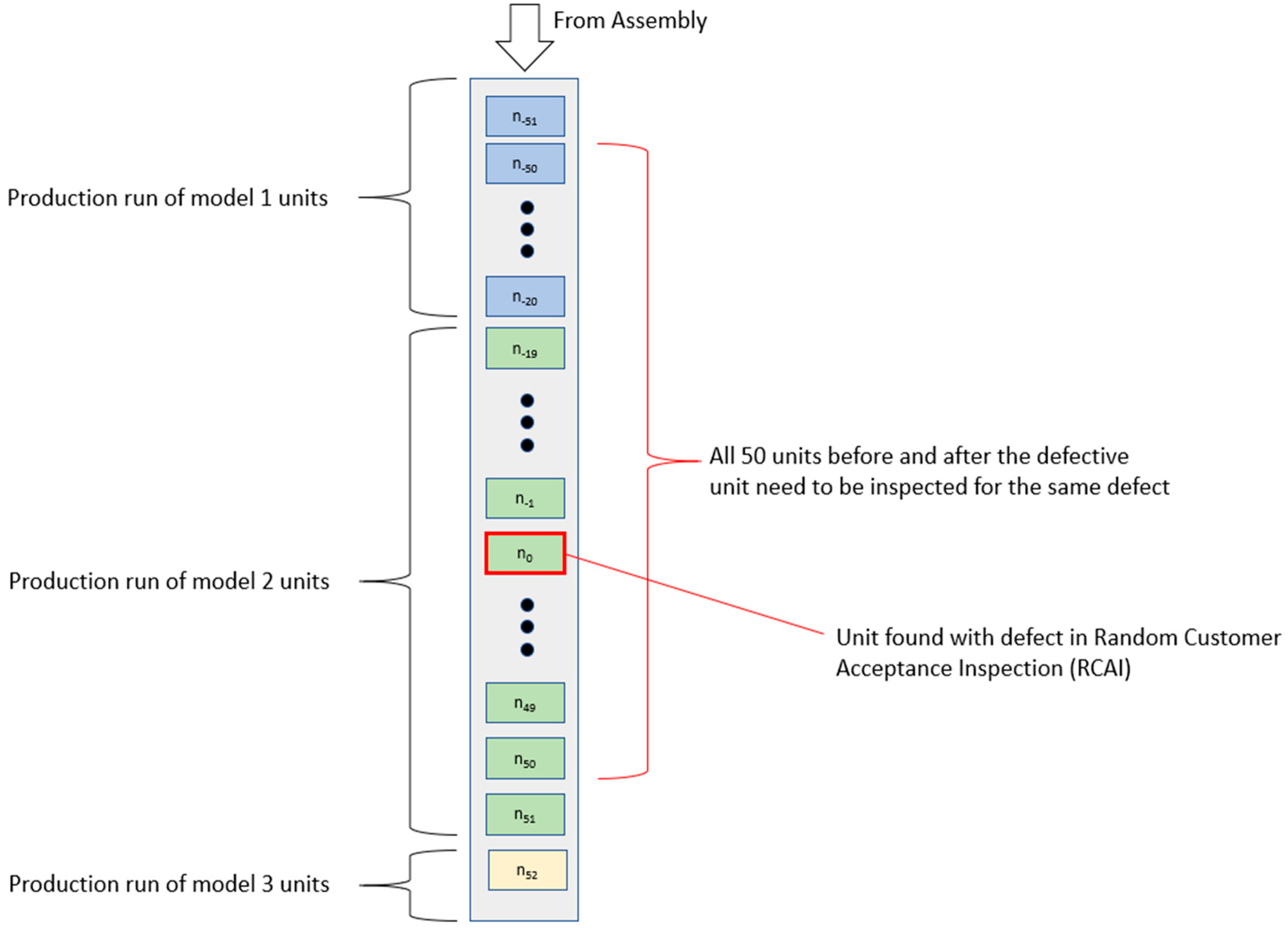
In order to formulate an effective approach to this problem, Figure 3 helps to visualize the key steps that correspond to each variable in the dataset on the production line. On the mixed model production line, units of a particular model are represented by color and, as depicted in the figure, there is a negligible changeover time between different models on a production that runs without pause. Data are collected at key points in the production line via barcode scanners and vision systems. Most of this data pertains to serial numbers and model numbers of units that pass through the production line at various stages or are redirected to testing and rework loops. Each production run of a particular model can vary widely in the number of units, from a few units of an experimental batch to several thousand that continue production over multiple days. Despite this, at no point is the production line stopped due to a model changeover.
Since the serial numbers are assigned sequentially to units on each line during assembly with zero loss of units before inspection, the unit’s serial numbers can be used to measure their relative position on the production with respect to other units in this study.
During RCAI, units found with defects are recorded on a separate dataset which includes additional quality-related information such as unit model, nature of defect, inspector identifiers, and all other units before and after that were marked for inspection regarding the same defect. The data points recorded in the RCAI dataset have fields that contain unrestricted string inputs. As such, they tend to require manual dissemination to structure into definable features that can be used for classification. Thus, each RCAI defect is categorized into a number of headings.
The top three categories accounting for RCAI defects are described as follows:
- 3.
- New Product Introduction (NPI) Defect. These are defects found on models that have been introduced into production recently and thus usually contain a large variety of defects caused by design oversights or frequent model revisions. This category stops being applied to defects once occurrence of such defects reaches acceptable thresholds. Thus, there is little need to train classification models to detect these since the categorization of their occurrence depends on their rate of occurrence and would result in a trivial discovery.
- 4.
- Aesthetic Issues. These RCAI defects pertain to superficial issues such as scratches, dents, or discolorations. Multiple factory studies in these issues had found process related deviations and other random human error to be the cause of such defects. However, since the dataset chosen does not contain manufacturing process parameters for each unit, it would seem rather difficult to train an accurate prediction model to classify such occurrences. Nonetheless, there is scope for such a study once the required data becomes available.
- 5.
- Wrong or Missing Parts. These refer to defects in which parts were missing from the final product or if wrong parts were assembled instead. Early discussions regarding these occurrences had suggested causes such as model changeovers, worker fatigue in late shift, complexity of certain product models, among others. Since there are abundant data regarding most of the suggested causes, it could be possible to train a classification model to predict these occurrences and test the validity of suggested causes. As such, RCAI defects exclusively categorized as Wrong/Missing Parts would be used as class variables in the classification model discussed in this paper.
Collection of assembly and fabrication process parameters via vision systems and tool metrics has been implemented on newer low-throughput lines but was still in process of being installed on the main assembly line studied in this paper. Despite the availability of many more features on the new line, the reason for using the high-throughput line instead is because of the fact that the newer lines do not operate at fixed speeds and also because they only account for about 5% of the total factory’s production as compared to the main line. Combined with the fact that each unit on the new lines is inspected and reworked on-the-spot with no guarantee of documentation, it would have made for a difficult task to build a classification model using the smaller and unreliable dataset available.
4. Results
These are the results of multiple classification models trained from the training dataset containing 60,508 instances and their resultant predictions on an independent test dataset containing 15,128 instances. The results pertain to various models trained from combinations of feature selection, feature construction, classification and hyperparameter tuning methods applied as per the workflow described in Figure 1.
All of the resulting models were trained from a dataset containing datapoints synthesized using SMOTE to address the massive class imbalance. Additionally, the same seed was set to ensure consistency regarding the cross-validation folds in order to better compare results.
All models were trained with the use of the caret, classification, and regression training R package by Max Kuhn, 2020 along with associated packages used for different classification models and visualization. On average, training the random forest models took 16.45 min and training the XGBoost models took 14.47 min.
Evaluation of the models was completed via Cohen’s Kappa (κ), derived from confusion matrices. Graphical representations of performance are also depicted in the form of ROC curves. Predicting the response of the independent test dataset took on average 0.32 s for random forest models and 0.05 s for XGBoost models.
4.1. Model A: Initial Classification with no Feature Construction or Selection
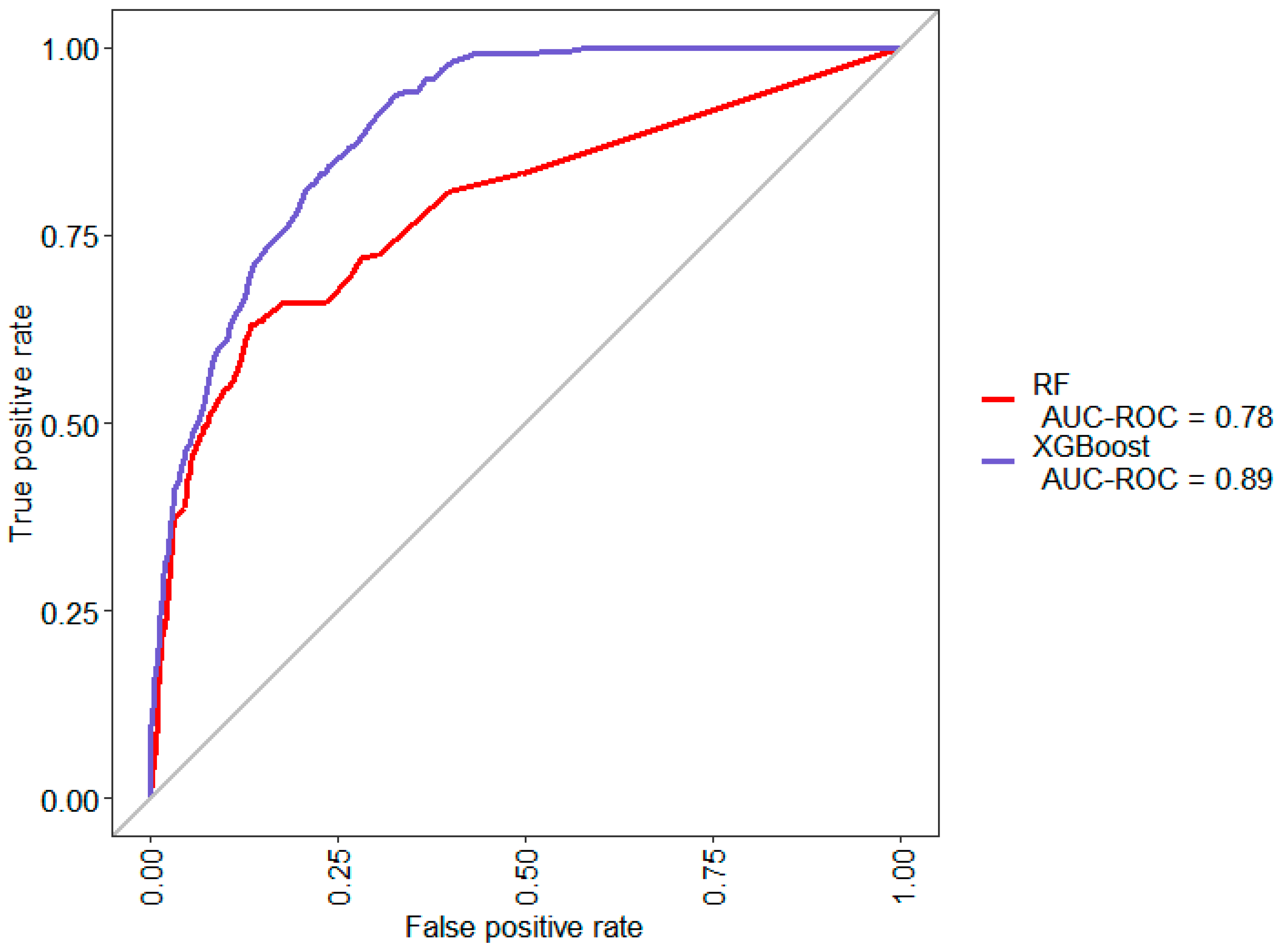
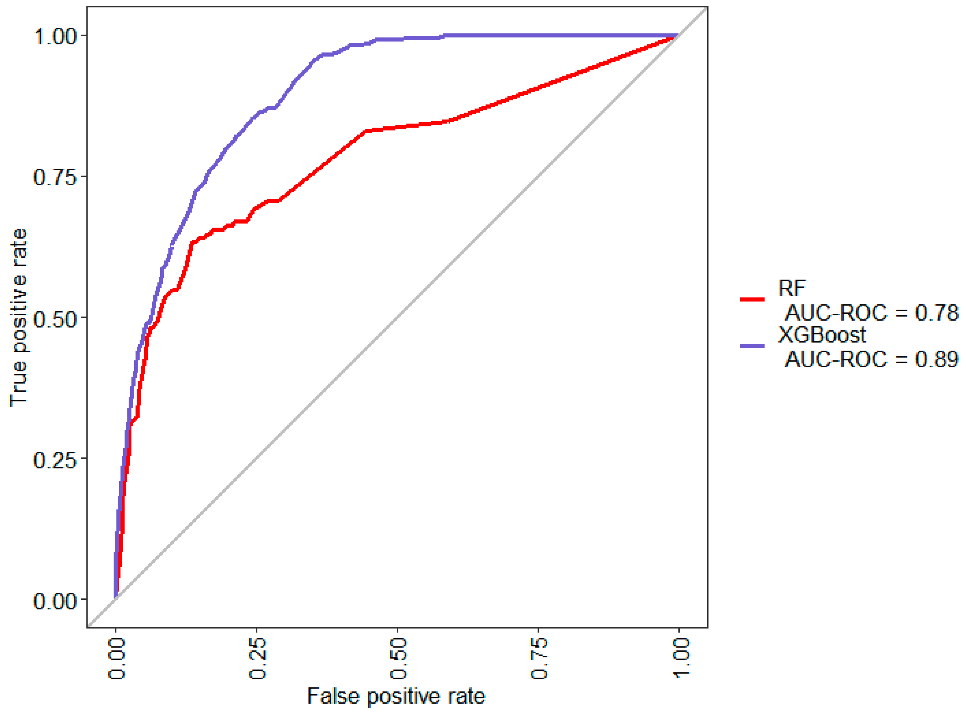
Model A was learned via random forest and XGBoost algorithm from the initially obtained clean dataset, with no feature selection or additional features constructed. Figure 4 and Table 3 show the results of its evaluation.
Despite the generally high accuracy derived from the confusion matrix, it does not indicate a good prediction model since the majority class accounts for 93.23% of the dataset. Thus, a random classifier would likely achieve similar or better accuracy.
The XGBoost classifier performs much better than the random forest classifier when it comes to predicting the minority class. However, it still fails to correctly predict 58.89% of the suspicious units from the test dataset.
Primarily, basic features like model or platform type were used in the initial classification to make predictions on the likelihood of defects. This would be similar to what a quality inspector would conclude based on knowledge of previous inspection data pertaining to problematic models or product platforms. However, a model like this would not be sufficient to make any decisions to change inspection strategies.
4.2. Model B: Classification with Model Changeover Feature
In order to explore some of the possible root causes discussed regarding RCAI defects, Model B was trained on a dataset in which irrelevant features like Seq.Number were removed. Additionally, a new feature, model_change is constructed in a manner similar to that described in this paper’s method section. The new feature denotes if a unit immediately follows another unit of different model in the production line. Figure 5 and Table 4 show the results of the changes.
There is a slight improvement in the performance of the random forest model and slight worsening of the XGBoost model, but this is mostly negligible in both cases and could be attributed to randomness.
Likely, the problem with the constructed feature is that only the first unit after each model changeover is marked whereas multiple suspicious units are identified after each RCAI failure. This is supported by the fact that even the minority class constitutes more data points than the constructed feature. Therefore, the constructed feature would be a heavy minority and would not result in significant improvements in the classification model.
4.3. Model C: Classification with Proximity to Model Changeover Feature
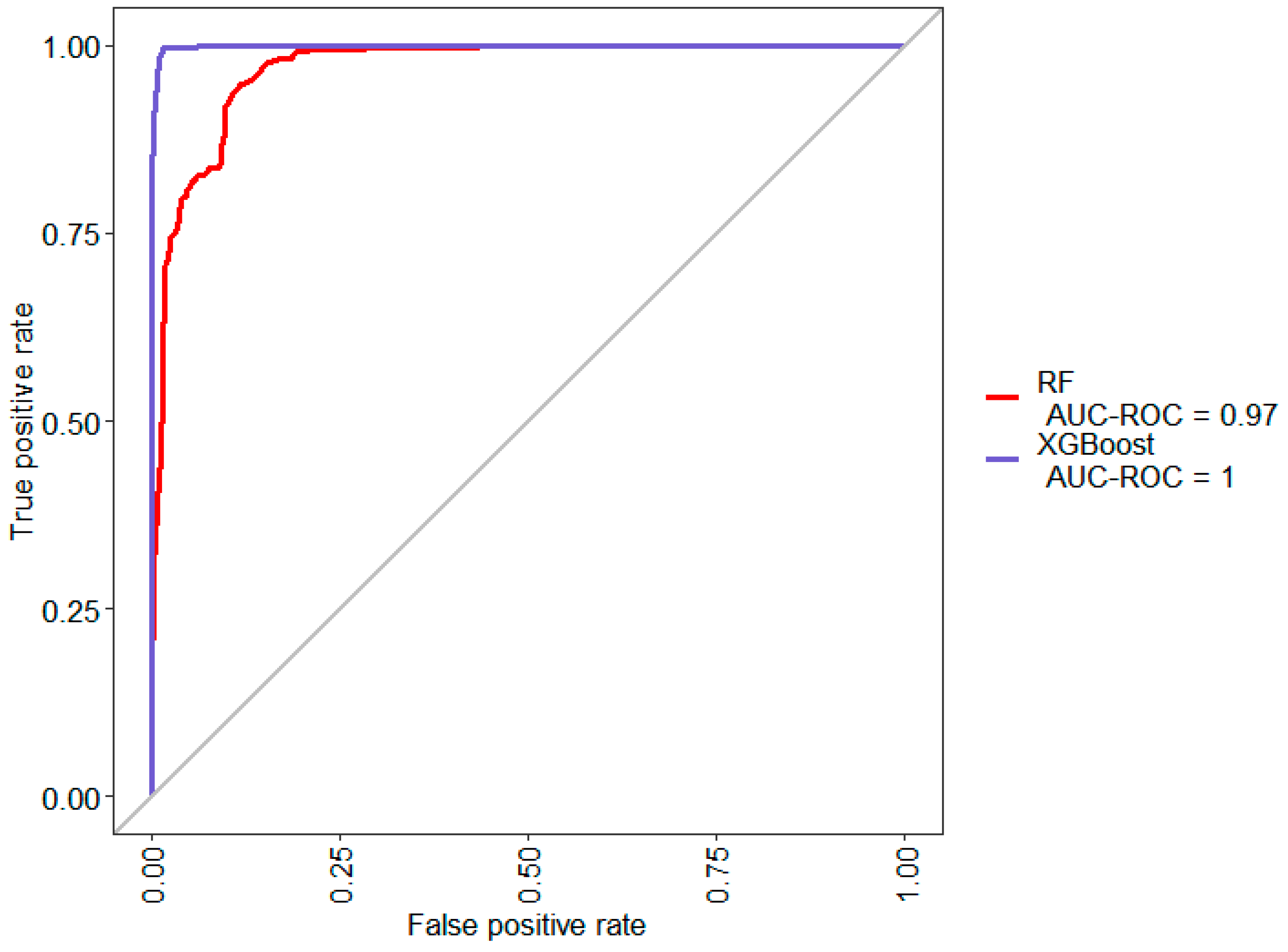
To correct the problem identified in Model B, another feature has been derived from the model_change feature for Model C, using the method described in this paper. This feature, batch_seq, represents the number of units between the product pertaining to the data point and the last unit which had model_change = 1. The results of training classification models with the newly constructed feature are shown in Figure 6 and Table 5.
The results show a significant improvement in the performance of both models in predicting the independent test dataset. The XGBoost model could predict suspected defective units with 98.34% accuracy. This likely confirms the correlation between model changeovers and the occurrence of RCAI defects that were categorized as missing or wrong parts.
The results also show the differences between boosting methods such as XGBoost and bagging methods like random forest. While bagging methods tend to suffer from increased bias, boosting methods tend to have less bias but suffer from overfitting. Table 5 shows the fact that despite the drastically improved performance as compared to the previous model, the random forest classifier still only classified 60.16% of the minority class correctly but had a bias towards classifying the majority class instead.
The XGBoost algorithm performed much better than the random forest classifier since it correctly predicted 98.34% of the minority class in the independent test dataset and had a comparable performance when evaluated within the cross-validation loop in the training dataset.
4.4. Model D: Classification with Normalized Proximity to Model Changeover Feature
Despite the success of Model C trained from the earlier constructed feature, the results could possibly be improved further by processing the constructed feature even more.
A limitation of the batch_seq feature constructed earlier is the fact that its value depends on the number of units between the product and previous model change. As such, in the factory with production runs of variable lengths, an adjusted measure of the unit’s position in the run could prove more helpful than an absolute measure like batch_seq.
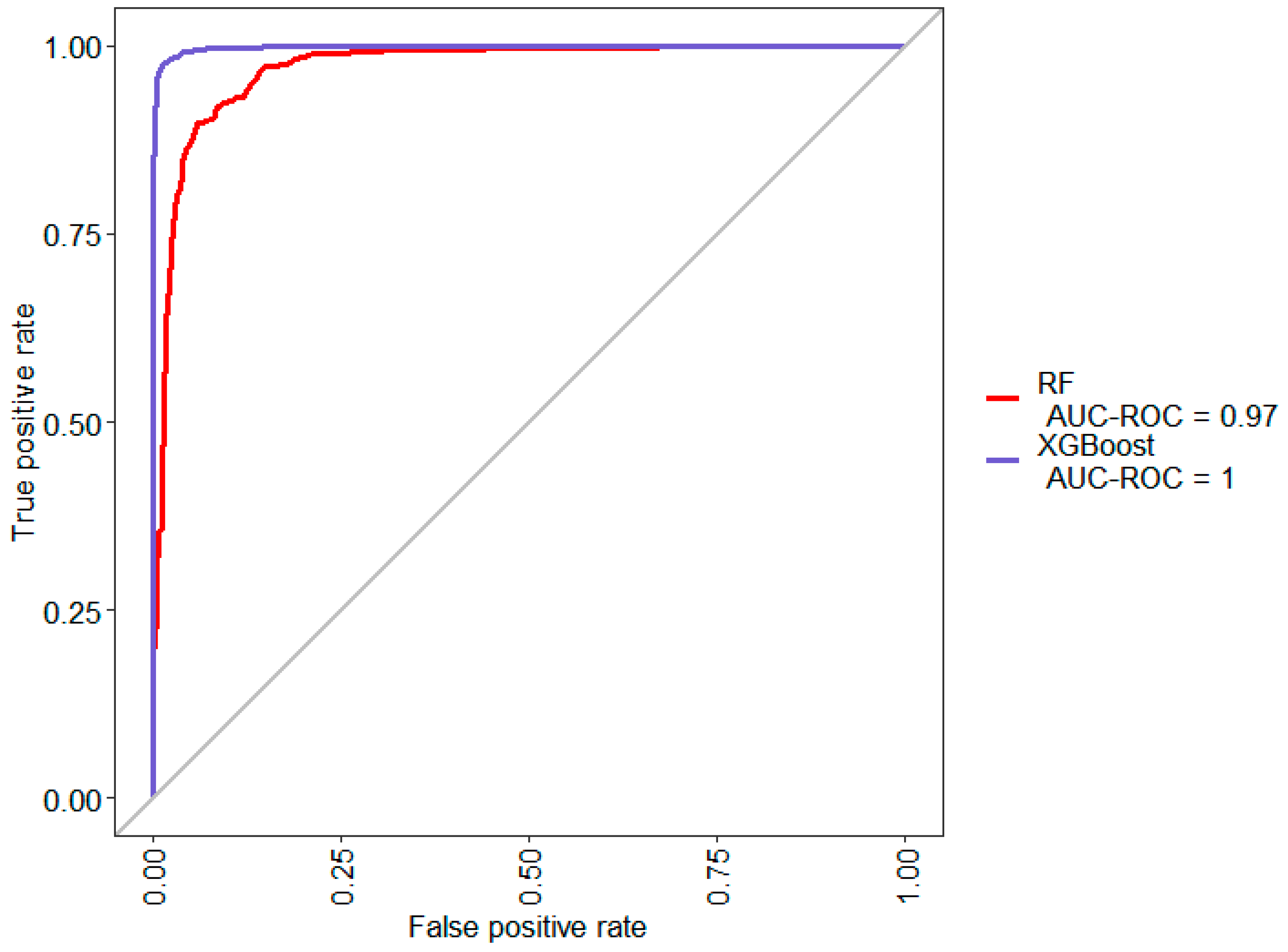
Thus, in Model D, the feature batch_seqperc is derived from batch_seq to replace it such that:
batch_seqperc = batch_seq/total units in production run
This feature accounts for production runs of varying size. Figure 7 and Table 6 show the results of training the classification models on the newly constructed batch_seqperc feature.
The results show slight improvement in the Cohen’s Kappa of the XGBoost model and a worsening of the random forest model. Both of the models become worse at predicting the minority class after using the batch_seqperc feature as opposed to the batch_seq feature.
This likely suggests that the class value of suspicious units can be better explained by an absolute measure of the unit’s position in the production run rather than an adjusted measure. Possibly, the occurrence of human error when assembling wrong parts in units is highest in the units immediately after model change regardless of the total number of units in the same-model production run.
5. Conclusions
Despite the common use of machine learning and data mining techniques at various stages of a supply chain, this paper’s results indicate that it is viable to use similar methods to predict compliance quality from data pertaining to multiple processes. The case study pertaining to a manufacturing industry provided a dataset that could be used to predict product containing wrong or missing parts with significant accuracy and Cohen’s Kappa, using the proposed method. Using production and quality data from the case studied, machine learning techniques were used to predict the compliance quality of a manufactured unit in the context of end inspection. With the increasing availability of process data due to Industry 4.0 implementations in modern manufacturing plants, future applications of the proposed method are likely to be successful. Thus, product compliance quality can be predicted as well as process-specific quality, with sufficiently large and feature-rich datasets available.
This paper builds upon similar research conducted regarding the application of machine learning in various manufacturing tasks, by expanding its scope to predict the overall compliance quality of product in final inspection of a production line. It also improves upon similar research in multistage manufacturing quality prediction by addressing class imbalance and the need for feature enrichment via feature engineering. The classification model trained from data pertaining to the case study can be used in its relevant factory to preemptively contain product units that would be defective due to wrong or missing parts in assembly, thus significantly saving on costs for product recalls and transportation due to escaped units. The prediction models could be trained in approximately 15 min using a personal computer whereas predictions took less than 1 s for 15,128 datapoints. The time required for training could vary significantly with the nature of the training dataset, algorithm and hyperparameters chosen but the time required to predict responses using the trained model was negligibly low for the case in this paper. Thus, the model could be trained in advance using the available data and prediction could be done in real-time. As such, this could provide an additional layer of quality control with relatively low investment in equipment or time.
The aim of this paper was to explore the use of machine learning to predict manufacturing compliance quality as per the outcome of quality inspections. It was possible to train a prediction model with defective unit prediction accuracy of 98.34%, overall accuracy of 98.78% and Cohen’s Kappa of 0.91, using a combination of feature construction and ensemble classification algorithms. The results obtained indicate that there is a significant improvement in the prediction model’s performance when it uses a dataset with features constructed to signify the position of each unit within the production line’s run of a product model. It also appears that using an absolute measure of the unit’s sequential order produced slightly better prediction of the minority class as compared to a normalized variable to represent the unit’s position in the batch.
The performance of the XGBoost model had been consistently better than that learned via random forest and significantly better at predicting the minority class. However, the case study in this paper indicates that regardless of the algorithm chosen, the trained model seemed to perform significantly better when specific features were constructed using prior domain knowledge regarding the nature of the dataset.
This study is subject to a few limitations, which suggests future research direction in the following: Firstly, for the case studied, improvement can be possible by constructing features to signify a change in model color or platform, similar to the model change. Other applications of the proposed method might require more features in order to obtain a prediction model with the required values of accuracy and Cohen’s Kappa. Secondly, analysis of the models to understand what caused quality defects can be conducted. This was not conducted due to the design of this study and availability of the data. Future studies using datasets with more features corresponding to manufacturing process data can be conducted to understand the causes for quality non-compliances as well as predictions. Thirdly, due to dataset limitations, only quality defects pertaining to products with wrong or missing parts could be feasibly predicted with the available features. With sufficient process data, machine learning methods researched in process-specific applications could be incorporated into end quality inspection as well. Finally, this paper did not explore the use of popularly used prediction algorithms such as neural networks due to the early success of the gradient boosting method and the fact that neural networks tend to perform better with larger and more feature-rich datasets, as opposed to that used in this paper’s case study. However, this suggests the possibility of future research to evaluate the performance of neural networks alongside algorithms used in this paper.
Author Contributions
Methodology, S.S.; writing—original draft preparation, S.S.; writing—review and editing, S.S. and G.H.; supervision, G.H. Both authors have read and agreed to the published version of the manuscript.
Funding
This research received no external funding.
Conflicts of Interest
The authors declare no conflict of interest.
References
- Campanella, J. Principles of Quality Costs: Principles, implementation, and use. In Proceedings of the ASQ World Conference on Quality and Improvement Proceedings; American Society for Quality: Milwaukee, WI, USA, 1999; p. 507. [Google Scholar]
- Moldovan, D.; Cioara, T.; Anghel, I.; Salomie, I. Machine learning for sensor-based manufacturing processes. In Proceedings of the 2017 13th IEEE International Conference on Intelligent Computer Communication and Processing (ICCP), Cluj-Napoca, Romania, 7–9 September 2017; IEEE: New York, NY, USA, 2017; pp. 147–154. [Google Scholar]
- Kerdprasop, K.; Kerdprasop, N. Feature selection and boosting techniques to improve fault detection accuracy in the semiconductor manufacturing process. In Proceedings of the World Congress on Engineering 2012, London, UK, 4–6 July 2012; International Association of Engineers (IAENG): Kowloon, China, 2010; Volume 2188, pp. 398–403. [Google Scholar]
- Kao, H.-A.; Hsieh, Y.-S.; Chen, C.-H.; Lee, J. Quality prediction modeling for multistage manufacturing based on classification and association rule mining. In Proceedings of the 2nd International Conference on Precision Machinery and Manufacturing Technology (ICPMMT), Kenting, Taiwan, 19–21 May 2017; EDP Sciences: Les Ulis, France, 2017; Volume 123. [Google Scholar]
- Arif, F.; Suryana, N.; Hussin, B. A data mining approach for developing quality prediction model in multi-stage manufacturing. Int. J. Comput. Appl. 2013, 69, 35–40. [Google Scholar] [CrossRef]
- Köksal, G.; Batmaz, İ.; Testik, M.C. A review of data mining applications for quality improvement in manufacturing industry. Expert Syst. Appl. 2011, 38, 13448–13467. [Google Scholar] [CrossRef]
- Saura, J.R. Using Data Sciences in Digital Marketing: Framework, methods, and performance metrics. J. Innov. Knowl. 2020. [Google Scholar] [CrossRef]
- Jain, A.K.; Murty, M.N.; Flynn, P.J. Data clustering: A review. ACM Comput. Surv. CSUR 1999, 31, 264–323. [Google Scholar] [CrossRef]
- Piatetsky-Shapiro, G. Discovery, analysis, and presentation of strong rules. Knowledge Discovery Databases 1991, 11, 229–238. [Google Scholar]
- Schuh, G.; Reinhart, G.; Prote, J.-P.; Sauermann, F.; Horsthofer, J.; Oppolzer, F.; Knoll, D. Data mining definitions and applications for the management of production complexity. Procedia CIRP 2019, 81, 874–879. [Google Scholar] [CrossRef]
- Kotsiantis, S.B.; Zaharakis, I.; Pintelas, P. Supervised machine learning: A review of classification techniques. Emerg. Artif. Intell. Appl. Comput. Eng. 2007, 160, 3–24. [Google Scholar]
- Scime, L.; Beuth, J. Anomaly detection and classification in a laser powder bed additive manufacturing process using a trained computer vision algorithm. Addit. Manuf. 2018, 19, 114–126. [Google Scholar] [CrossRef]
- Moretti, C.; Steinhaeuser, K.; Thain, D.; Chawla, N.V. Scaling up classifiers to cloud computers. In Proceedings of the 2008 Eighth IEEE International Conference on Data Mining, Pisa, Italy, 15–19 December 2008; IEEE: New York, NY, USA, 2008; pp. 472–481. [Google Scholar]
- Fernández, A.; García, S.; Herrera, F. Addressing the classification with imbalanced data: Open problems and new challenges on class distribution. In Proceedings of the 6th International conference on hybrid artificial intelligence systems, Wroclaw, Poland, 23–25 May 2011; Springer: Berlin/Heidelberg, Germany, 2011; pp. 1–10. [Google Scholar]
- Kim, A.; Oh, K.; Jung, J.-Y.; Kim, B. Imbalanced classification of manufacturing quality conditions using cost-sensitive decision tree ensembles. Int. J. Comput. Integr. Manuf. 2018, 31, 701–717. [Google Scholar] [CrossRef]
- Zhu, H.; Liu, G.; Zhou, M.; Xie, Y.; Abusorrah, A.; Kang, Q. Optimizing Weighted Extreme Learning Machines for Imbalanced Classification and Application to Credit Card Fraud Detection. Neurocomputing 2020. [Google Scholar] [CrossRef]
- Jia, F.; Lei, Y.; Lu, N.; Xing, S. Deep normalized convolutional neural network for imbalanced fault classification of machinery and its understanding via visualization. Mech. Syst. Signal. Process. 2018, 110, 349–367. [Google Scholar] [CrossRef]
- Zhang, X.; Wei, X.; Li, F.; Hu, F.; Jia, W.; Wang, C. Fuzzy Support Vector Machine with Imbalanced Regulator and its Application in Stroke Classification. In Proceedings of the 2019 IEEE Fifth International Conference on Big Data Computing Service and Applications (BigDataService), Newark, CA, USA, 4–9 April 2019; IEEE: New York, NY, USA, 2019; pp. 290–295. [Google Scholar]
- Mahanipour, A.; Nezamabadi-Pour, H. Improved PSO-based feature construction algorithm using Feature Selection Methods. In Proceedings of the 2017 2nd Conference on Swarm Intelligence and Evolutionary Computation (CSIEC), Kerman, Iran, 7–9 March 2017; IEEE: New York, NY, USA, 2017; pp. 1–5. [Google Scholar]
- Chawla, N.V.; Bowyer, K.W.; Hall, L.O.; Kegelmeyer, W.P. SMOTE: Synthetic minority over-sampling technique. J. Artif. Intell. Res. 2002, 16, 321–357. [Google Scholar] [CrossRef]
- Tao, X.; Li, Q.; Guo, W.; Ren, C.; Li, C.; Liu, R.; Zou, J. Self-adaptive cost weights-based support vector machine cost-sensitive ensemble for imbalanced data classification. Inf. Sci. 2019, 487, 31–56. [Google Scholar] [CrossRef]
- Feng, W.; Dauphin, G.; Huang, W.; Quan, Y.; Liao, W. New margin-based subsampling iterative technique in modified random forests for classification. Knowl. Based Syst. 2019, 182, 104845. [Google Scholar] [CrossRef]
- Faris, H.; Abukhurma, R.; Almanaseer, W.; Saadeh, M.; Mora, A.M.; Castillo, P.A.; Aljarah, I. Improving financial bankruptcy prediction in a highly imbalanced class distribution using oversampling and ensemble learning: A case from the Spanish market. Prog. Artif. Intell. 2020, 9, 31–53. [Google Scholar] [CrossRef]
- Zhao, H.; Sinha, A.P.; Ge, W. Effects of feature construction on classification performance: An empirical study in bank failure prediction. Expert Syst. Appl. 2009, 36, 2633–2644. [Google Scholar] [CrossRef]
- Muñoz, E.; Capón-García, E. Systematic approach of multi-label classification for production scheduling. Comput. Chem. Eng. 2019, 122, 238–246. [Google Scholar] [CrossRef]
- Bodunov, O.; Schmidt, F.; Martin, A.; Brito, A.; Fetzer, C. Real-time Destination and ETA Prediction for Maritime Traffic. In Proceedings of the 12th ACM International Conference on Distributed and Event-based Systems, Hamilton, New Zealand, 25–29 June 2018; ACM: New York, NY, USA, 2018; pp. 198–201. [Google Scholar]
- Esbensen, K.H.; Geladi, P. Principles of proper validation: Use and abuse of re-sampling for validation. J. Chemom. 2010, 24, 168–187. [Google Scholar] [CrossRef]
- Kohavi, R. A study of cross-validation and bootstrap for accuracy estimation and model selection. In Proceedings of the 1995 IJCAI 14th International Joint Conference on Artificial Intelligence, Montreal, QC, Canada, 20–25 August 1995; IJCAI: Saxony, Germany, 1995; Volume 14, pp. 1137–1145. [Google Scholar]
- Lan, H.; Pan, Y. A crowdsourcing quality prediction model based on random forests. In Proceedings of the 2019 IEEE/ACIS 18th International Conference on Computer and Information Science (ICIS), Beijing, China, 12–14 June 2019; IEEE Computer Society: Washington, DC, USA, 2019; pp. 315–319. [Google Scholar]
- Chen, T.; Guestrin, C. Xgboost: A scalable tree boosting system. In Proceedings of the 22nd Acm Sigkdd International Conference on Knowledge Discovery and Data Mining, San Francisco, CA, USA, 13–17 August 2016; ACM: New York, NY, USA, 2016; pp. 785–794. [Google Scholar]
- Xu, H.; Wang, H. Identifying diseases that cause psychological trauma and social avoidance by Xgboost. In Proceedings of the 2019 IEEE International Conference on Bioinformatics and Biomedicine (BIBM), San Diego, CA, USA, 18–21 November 2019; IEEE: New York, NY, USA, 2019; pp. 1809–1813. [Google Scholar]
- Yang, L.; Li, Y.; Di, C. Application of XGBoost in Identification of Power Quality Disturbance Source of Steady-state Disturbance Events. In Proceedings of the 2019 IEEE 9th International Conference on Electronics Information and Emergency Communication (ICEIEC), Beijing, China, 12–14 July 2019; IEEE: New York, NY, USA, 2019; pp. 1–6. [Google Scholar]
- Drucker, H.; Burges, C.J.; Kaufman, L.; Smola, A.J.; Vapnik, V. Support vector regression machines. In Advances in Neural Information Processing Systems; MIT Press: Cambridge, MA, USA, 1997; pp. 155–161. [Google Scholar]
- Tan, Y.; Xia, Y.; Wang, J. Neural network realization of support vector methods for pattern classification. In Proceedings of the IEEE-INNS-ENNS International Joint Conference on Neural Networks. IJCNN 2000. Neural Computing: New Challenges and Perspectives for the New Millennium, Como, Italy, 27 July 2000; IEEE: New York, NY, USA, 2000; Volume 6, pp. 411–416. [Google Scholar]
- Cheldelin, B.; Ishii, K. Mixed-model assembly quality: An approach to prevent human errors. In Proceedings of the ASME International Mechanical Engineering Congress and Exposition, Anaheim, CA, USA, 13–19 November 2004; ASME: New York, NY, USA, 2004; Volume 47055, pp. 109–119. [Google Scholar]
- Neumann, W.P.; Kolus, A.; Wells, R.W. Human factors in production system design and quality performance—A systematic review. IFAC Pap. 2016, 49, 1721–1724. [Google Scholar] [CrossRef]
- Hasan, M.; Ibrahimy, M.; Motakabber, S.; Shahid, S. Classification of Multichannel EEG Signal by Single Layer Perceptron Learning Algorithm. In Proceedings of the 2014 International Conference on Computer and Communication Engineering, Kuala Lumpur, Malaysia, 23–25 September 2014; IEEE: New York, NY, USA, 2014; pp. 255–257. [Google Scholar]
- Chinchor, N.; Sundheim, B.M. MUC-5 Evaluation Metrics. In Proceedings of the Fifth Message Understanding Conference (MUC-5), Baltimore, MD, USA, 25–27 August 1993. [Google Scholar]
- Chicco, D.; Jurman, G. The advantages of the Matthews correlation coefficient (MCC) over F1 score and accuracy in binary classification evaluation. BMC Genom. 2020, 21, 6. [Google Scholar] [CrossRef] [Green Version]
- Vieira, S.M.; Kaymak, U.; Sousa, J.M. Cohen’s kappa coefficient as a performance measure for feature selection. In Proceedings of the International Conference on Fuzzy Systems, Barcelona, Spain, 18–23 July 2010; IEEE: New York, NY, USA, 2010; pp. 1–8. [Google Scholar]
- Chou, P.B.; Rao, A.R.; Sturzenbecker, M.C.; Wu, F.Y.; Brecher, V.H. Automatic defect classification for semiconductor manufacturing. Mach. Vis. Appl. 1997, 9, 201–214. [Google Scholar] [CrossRef]
Figure 1.
Method overview.

Figure 2.
Confusion matrix for a binary class with negative (no) and positive (yes) values. TN denotes true negative, FN denotes false negative, FP denotes false positive, and TP denotes true positive predictions.
Figure 2.
Confusion matrix for a binary class with negative (no) and positive (yes) values. TN denotes true negative, FN denotes false negative, FP denotes false positive, and TP denotes true positive predictions.

Figure 3.
A depiction of the inspection and containment process for suspected units after one is found defective in RCAI.
Figure 3.
A depiction of the inspection and containment process for suspected units after one is found defective in RCAI.

Figure 4.
ROC curves for the results of XGBoost and random forest classifiers without any constructed features.
Figure 4.
ROC curves for the results of XGBoost and random forest classifiers without any constructed features.

Figure 5.
ROC curves for the results of XGBoost and Random Forest Classifiers using model_change feature.
Figure 5.
ROC curves for the results of XGBoost and Random Forest Classifiers using model_change feature.

Figure 6.
ROC curves for the results of XGBoost and Random Forest Classifiers using batch_seq feature.
Figure 6.
ROC curves for the results of XGBoost and Random Forest Classifiers using batch_seq feature.

Figure 7.
ROC curves for the results of XGBoost and Random Forest Classifiers using batch_seqperc feature.
Figure 7.
ROC curves for the results of XGBoost and Random Forest Classifiers using batch_seqperc feature.


Table 1.
A table describing the meaning of fields available in the raw dataset.
| Variable Name | Description |
|---|---|
| Sequence Number | This is the serial number of each unit and serves as a unique sequential identifier in the production line. |
| Model | This is the model number of the unit passing through the production line. |
| Week | This is the week number at which the unit entered final inspection. |
| Color | Describes the color of the unit. This tends to get recorded as a derivative of the model number. |
| BrandGroup | Describes the make of the unit. Derived from Model |
| PlatformGroup | Platforms are used to group models with similar, discernible features. For example, a mountain bicycle and stunt bike can be easily distinguished |
| RCAIDefect | This denotes a unit found defective in RCAI for Wrong/Missing parts as 1, and 0 otherwise. |
| SuspiciousUnit | This binary variable denotes all of the approximately 50 units before and after the RCAI defective unit which are marked for inspection of similar issues. |
Table 2.
Variable distribution of the two possible class variables.
| RCAIDefect Value | Datapoints | SuspiciousUnit Value | Datapoints |
|---|---|---|---|
| 0 | 75,584 | 0 | 70,501 |
| 1 | 52 | 1 | 5135 |
Table 3.
Confusion matrices for the test results of XGBoost and random forest classifiers without any constructed features.
Table 3.
Confusion matrices for the test results of XGBoost and random forest classifiers without any constructed features.
| Random Forest | XGBoost | ||||||
|---|---|---|---|---|---|---|---|
| Reference | Reference | ||||||
| No | Yes | No | Yes | ||||
| Prediction | No | 13,916 | 855 | Prediction | No | 13,632 | 603 |
| Yes | 188 | 169 | Yes | 472 | 421 | ||
| Accuracy: 0.9311 | Accuracy: 0.9289 | ||||||
| Cohen’s Kappa: 0.2174 | Cohen’s Kappa: 0.4015 | ||||||
Table 4.
Confusion matrices for the test results of XGBoost and Random Forest Classifiers using model_change feature.
Table 4.
Confusion matrices for the test results of XGBoost and Random Forest Classifiers using model_change feature.
| Random Forest | XGBoost | ||||||
|---|---|---|---|---|---|---|---|
| Reference | Reference | ||||||
| No | Yes | No | Yes | ||||
| Prediction | No | 13,907 | 833 | Prediction | No | 13,657 | 627 |
| Yes | 197 | 191 | Yes | 447 | 397 | ||
| Accuracy: 0.9319 | Accuracy: 0.9290 | ||||||
| Cohen’s Kappa: 0.2424 | Cohen’s Kappa: 0.3876 | ||||||
Table 5.
Confusion matrices for the test results of XGBoost and Random Forest Classifiers using batch_seq feature.
Table 5.
Confusion matrices for the test results of XGBoost and Random Forest Classifiers using batch_seq feature.
| Random Forest | XGBoost | ||||||
|---|---|---|---|---|---|---|---|
| Reference | Reference | ||||||
| No | Yes | No | Yes | ||||
| Prediction | No | 13,882 | 408 | Prediction | No | 13,937 | 17 |
| Yes | 222 | 616 | Yes | 167 | 1007 | ||
| Accuracy: 0.9584 | Accuracy: 0.9878 | ||||||
| Cohen’s Kappa: 0.6397 | Cohen’s Kappa: 0.9098 | ||||||
Table 6.
Confusion matrices for the test results of XGBoost and Random Forest Classifiers using batch_seqperc feature.
Table 6.
Confusion matrices for the test results of XGBoost and Random Forest Classifiers using batch_seqperc feature.
| Random Forest | XGBoost | ||||||
|---|---|---|---|---|---|---|---|
| Reference | Reference | ||||||
| No | Yes | No | Yes | ||||
| Prediction | No | 13,900 | 558 | Prediction | No | 13,970 | 36 |
| Yes | 204 | 466 | Yes | 134 | 988 | ||
| Accuracy: 0.9496 | Accuracy: 0.9888 | ||||||
| Cohen’s Kappa: 0.5247 | Cohen’s Kappa: 0.9147 | ||||||
Publisher’s Note: MDPI stays neutral with regard to jurisdictional claims in published maps and institutional affiliations. |
© 2020 by the authors. Licensee MDPI, Basel, Switzerland. This article is an open access article distributed under the terms and conditions of the Creative Commons Attribution (CC BY) license (http://creativecommons.org/licenses/by/4.0/).
Share and Cite
MDPI and ACS Style
Sankhye, S.; Hu, G. Machine Learning Methods for Quality Prediction in Production. Logistics 2020, 4, 35. https://0-doi-org.brum.beds.ac.uk/10.3390/logistics4040035
AMA Style
Sankhye S, Hu G. Machine Learning Methods for Quality Prediction in Production. Logistics. 2020; 4(4):35. https://0-doi-org.brum.beds.ac.uk/10.3390/logistics4040035
Chicago/Turabian StyleSankhye, Sidharth, and Guiping Hu. 2020. "Machine Learning Methods for Quality Prediction in Production" Logistics 4, no. 4: 35. https://0-doi-org.brum.beds.ac.uk/10.3390/logistics4040035