


Design and Evaluation of an Integrated Autonomous Control Method for Automobile Terminals

1
Planning and Control of Production and Logistics Systems (PSPS), Faculty of Production Engineering, University of Bremen, c/o BIBA, Hochschulring 20, 28359 Bremen, Germany
2
BIBA—Bremer Institut für Produktion und Logistik, Hochschulring 20, 28359 Bremen, Germany
*
Author to whom correspondence should be addressed.
Logistics 2022, 6(4), 73; https://0-doi-org.brum.beds.ac.uk/10.3390/logistics6040073
Submission received: 6 September 2022
/
Revised: 29 September 2022
/
Accepted: 10 October 2022
/
Published: 13 October 2022
(This article belongs to the Special Issue Optimization and Management in Maritime Transportation)
Abstract
:Background: Automobile terminals play a key role in global finished car supply chains. Due to their connecting character between manufacturers on the one side and distributers on the other side, they are continuously faced with volatile demand fluctuations and unforeseen dynamic events, which cannot be handled adequately by existing planning methods. Autonomous control concepts already showed promising results coping with such dynamics. Methods: This paper describes the causes of dynamics and the terminal systems’ inherent shortcomings in dealing with such dynamics. On this basis, it derives terminal’s demand for novel planning approaches and presents a new integrated autonomous control method for automobile terminals. This novel autonomous control approach combines yard and berth assignments. This paper evaluates the performance of the new approach in a small comprehensive generic scenario. It compares classical planning approaches with the new autonomous control approach, by using a discrete event simulation model. Moreover, it analyses all relevant parameters of the new approach in a full factorial experiment design. In a second step this paper proves the applicability of the combined autonomous control approach to real-world terminals. It presents a simulation model of a real-world terminal and compares the new method with the existing terminal planning approaches. Results: This paper will show that the autonomous control approach is capable of outperforming existing centralized planning methods. In the generic and in the real-world case the new combined method leads to the best logistic target achievement. Conclusions: The new approach is highly suitable to automobile terminal systems and helps to overcome existing shortcomings. Especially in highly dynamic and complex settings, autonomous control performs better than conventional yard planning approaches.
1. Introduction
During recent years, an increasing trend in global vehicle production and distribution volumes could be observed until the outbreak of the COVID-19 pandemic in 2020 [1]. This trend led to high and dynamic utilization of storage and buffering capacities in entire global finished cars supply chains (SC). The outbreak of the COVID-19 pandemic fostered this trend and led to new dynamics in the entire automotive SC [2]. Due to suddenly decreasing sales volumes, vehicle manufacturers (OEMs) had a high demand for additional storage capacities and started to strategically strengthen local decentralized distribution structures in the whole SC [3]. This challenges all participants of the SC and forces them to adapt quicker to changing SC dynamics.
Automobile terminals play a key role in these SCs. They act as a direct hub for overseas transport and offer additional storage capacities [4]. Automobile terminals provide handling processes (i.e., loading and unloading of cars from transport carriers), storage processes, and technical service processes [5]. OEMs as focal companies of SCs directly trigger most of the terminal outbound processes as a kind of pull process, while inbound processes have characteristics of typical order neutral push processes. Dias et al., 2010 describe automobile terminals as classical decoupling points in the automotive SC with parallel occurring push and pull processes [6]. This decoupling generates on the one hand a higher degree of flexibility for the entire SC. On the other hand, it leads to a higher planning complexity of the terminal’s internal processes due to incomplete information. This especially affects classical yard planning and berth planning tasks, which both aim at minimizing driving distances (the distance between arrival areas, storage area, and final exit points) of cars. Conventional yard planning approaches assign groups of cars to pre-defined parking areas (e.g., sorted by manufacturer, model, and destination) based on order neutral forecast information [7,8]. Based on the yard assignment, classical berth planning approaches focus on reducing driving distances (or handling times) by allocating ships to suitable berths, which offer short routes between storage areas and ships [5,9]. These approaches ensure good assignment results in less dynamic and volatile situations. With increasing dynamics (e.g., caused by decisions of OEMs or externally caused weather-related delays), conventional approaches lead to worse assignments and long driving distances. As a consequence, plans get prone to forecast deviations and unforeseen events [8,10]. The implementation of autonomously controlled processes may be a promising approach to cope with these dynamics. In the context of automobile terminals, autonomous control showed already general applicability [11,12]. First approaches for an autonomously controlled yard assignment improve the systems performance under highly dynamic conditions [12,13]. However, existing studies did not investigate the possible potential of an integrated autonomous control approach for yard and berth assignment. Moreover, a systematic understanding of all autonomous control methods parameters impacting on the terminal performance is still missing. The transferability of autonomously controlled yard and berth assignment in real-word scale terminals is still an open question, as well.
Thus, this paper refines an existing autonomous control method for yard assignment decisions and extends this method to an integrated yard and berth assignment approach. It will evaluate this new method firstly in a comprehensive generic terminal scenario. In a first step it will compare the new method with conventional approaches. Subsequently, it will investigate the impact of all methods parameters with a full factorial experiment design. In a second step, this paper introduces a computer simulation model of a real-world automobile terminal. It will prove the method’s applicability in a real case and will show that the new methods are capable of outperforming conventional yard and berth assignment approaches.
Therefore, this paper is structured as follows: Section 2 discusses the planning processes of automobile terminals and presents the concept of an autonomous control as an approach to address the planning system’s inherent shortcomings. Subsequently, Section 3 introduces the modelling of automobile terminals and derives the new autonomous control method and discusses relevant parameters. On this basis, Section 4 presents the simulation results for a generic terminal model and evaluates the new method in depth, focusing on all parameters and their interactions. Moreover, it proves the transferability of the approach to real-world terminals. Therefore, it presents and discusses the simulation results for an exemplary case of one of the world’s largest automobile terminals. The analysis compares the autonomous control method with a conventionally planned situation by using historical data. Section 5 gives a summary and ends with an outlook for further research directions.
2. State of the Art
The concept of autonomously controlled logistics processes is closely connected to the idea of self-organizing systems. It is a meta-approach that can be applied to a broad range of logistics applications. This section addresses classical planning processes of automobile terminals, discusses inherent shortcomings of these conventional approaches, and presents how the concept of autonomous control may help to improve terminals logistics performance.
2.1. Planning Process of Automobile Terminals
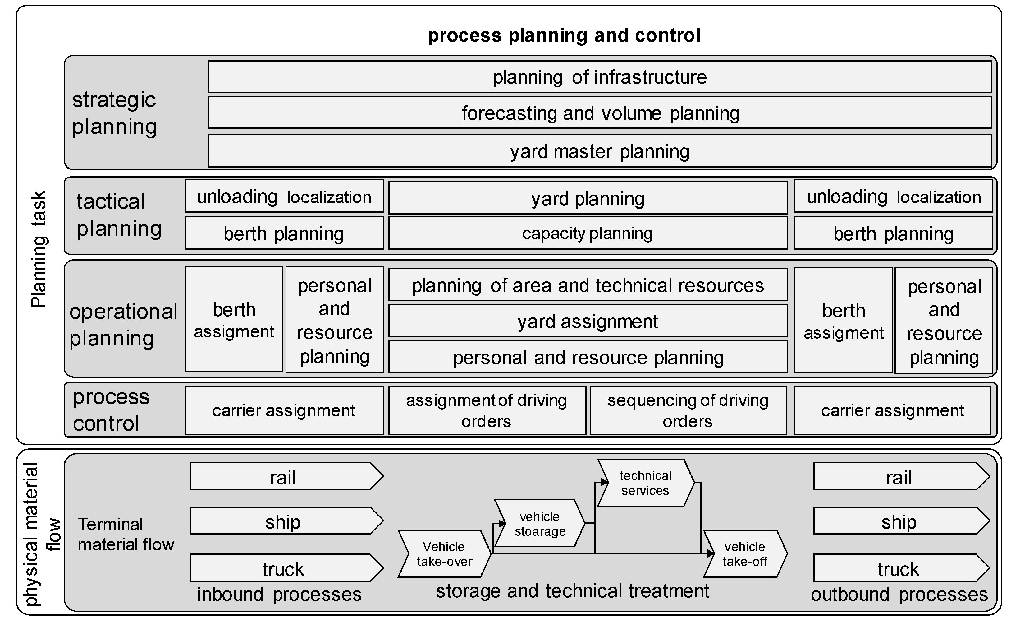
The physical movement and storage of vehicles is the main task of an automobile terminal. For organizing these functions, terminals offer a sequence of generic sub-processes (e.g., loading, technical treatment, or storage operations) [5]. Figure 1 shows these processes (bottom) about all necessary planning steps on different time scales. Normally, the material flow starts with unloading operations from different carriers (ship, rail, truck) followed by storage operations. Some terminals offer technical treatments for cars (e.g., interior modifications or repair of transport damage) [14,15]. After consolidating at the compound cars leave the terminal with different carriers (e.g., ship).
The overall objective of planning processes is organizing an efficient operation and the provision of planning tasks on different time scales [16]. On a long-term basis, the strategic planning focuses on the general setup, addressing infrastructure (e.g., additional berth or yard extensions) and yard master planning (e.g., basic rules for assignment of cars to yard areas). Long-term volume forecasts are used for this task [5,16]. A result of the long-term yard master planning is a rough assignment of estimated vehicle volumes to parking areas, which will be refined in the subsequent tactical phase. Based on more specific information (e.g., model-destination split or volume-related model-split) tactical planning refines this yard assignment [5]. All planning tasks aim at minimizing driving distances, reducing the handling times and at increasing the sorting of vehicle groups [8,9]. In this context sorting means minimizing the mixture of car groups (e.g., groups can be defined by attributes like OEMs, model type and shipment destination) traveling to different destinations. This helps to avoid additional handling movements for defragmenting yard areas. For the minimization of driving distances, both inbound and outbound planning aim at the assignment of carriers (i.e., ships, rail, and trucks) and the assignment of storage areas (yard planning), which lead to short routes. Especially, the ships’ assignment to berths during the berth allocation planning has a significant impact on overall handling times and driving distances [9,17]. The efficient solving of berth allocation problems (BAP) is a crucial task for ports in general [18]. Literature provides many approaches to a solution, especially for container terminals under deterministic or uncertain conditions (e.g., [19,20,21]). However, requirements for automobile terminals differ from those for container terminals. Dkhil et al., 2021 formulate a specific bi-objective optimization for automobile terminals (ATT-BAP), which aims at minimizing handling times and the crossing of car flows [9].
The operative planning phase refines these results on the highest level of detail when all information is available. In contrast to tactical planning, this phase is based on customer data (e.g., cars to be moved or ships’ fixed departure times). It augments the results of previous steps in pre-defined turns or with rolling time horizons on a short-term (daily or shift-wise) basis [14]. The operative planning process assigns personal resources to tasks and generates precise schedules [22,23]. As indicated in Figure 1, the planning process is a sequence of order neutral and order-driven tasks. Dias et al., 2010 describe these parallel order neutral push and customer-related pull processes as a classical decoupling point in a supply chain [6]. Like in other supply chains, decoupling points allow supply chains to react flexibly to market demand fluctuations and thus, may offer completive advantages to the whole supply chain. However, the occurrence of a decoupling point leads to increasingly complex internal dynamics for affected upstream and downstream operations [24,25]. Order neutral planned processes, like the assignment of incoming cars, refer only to forecast-based rules. Hence, only during the operative planning phase unforeseen dynamics like varying arrival volumes or postponed ship arrivals can be addressed directly. Thus, operative planning in most cases can only mitigate the effect on productivity by optimizing the berth allocation. This systematic drawback, resulting from the temporal interplay between rigid order neutral planning rules and order-driven planning steps (like berth allocations), opens the potential to improve the terminals productivity. In this regard, a more adaptive and dynamical adjustment of yard and berth assignments may increase the terminals’ capability to react to highly dynamic situations. An integration of both planning tasks may help to decrease total driving distances and may increase productivity.
2.2. Autonomous Control for Coping with Dynamics and Complexity
Autonomous control of logistics processes offers a generic approach to cope with increasing dynamics and systems complexity [26]. This concept, coming from the idea of self-organizing systems, propagates a shift of decision-making capabilities from centralized planning instances to the elements of the system. Accordingly, intelligent logistics objects can interact with others to gather information about current local system states and can make local decisions [26,27]. These objects may be physical objects in the system (e.g., machines on a shop floor [28], cars in a compound [13] or immaterial objects like production orders). The general idea behind this concept is affecting the performance of the system positively by changing its behavior due to local interactions and autonomously made decisions. Ideally, the dynamic interplay of autonomous objects causes positive emergence and allows robust systems behavior against dynamic disturbances [29]. The application of autonomous control methods showed already promising results in several fields of logistics (e.g., production [30,31], transport logistics [32], and terminal logistics [11,12]). However, the design and the implementation of autonomous control methods differs regarding the intelligent logistics objects and the decision process. Martins et al., 2020 [33] analyze autonomous control in production logistics and suggest a classification in rational, bio-inspired, and social inspired methods. Scholz-Reiter et al., 2010 [31] propose a similar classification, but they introduce a further differentiation regarding the horizon of the information collection of objects in terms of local information methods and information discovery methods. According to this classification, local information methods comprise rational and bio-inspired methods. Rational methods allow local decisions based on rational measures (e.g., estimated waiting times or due date punctuality). By contrast, bio-inspired strategies aim at transferring strategies from natural systems (e.g., ants’ [28] or bees’ foraging behavior [34]) to decision-making in logistics systems. Both types of methods have in common that their information usage is locally limited, and that they do not take system states that are far in the future into account. Information discovery methods aim to collect further information beyond the local scope for decision-making processes. They are inspired by modern communication protocols. Literature provides approaches for production (e.g., [31]) and transport logistics (e.g., [32]).
Based on a deep literature review, Martins et al., 2020 state that rational and information discovery methods outperform bio-inspired methods in the context of production logistics. During the operative production process, all relevant information (like production variants and related processing times) is known in advance. Accordingly, methods directly using this information usually perform better than methods indirectly using the information as bounded rational methods do in production systems [29].
Regarding terminal processes, this domination of rational strategies changes. As described above, terminal processes are characterized by incomplete information, which must be anticipated during operation. In this context, bounded rational strategies like pheromone-based methods may use this as their key advantage: these methods use the information of past-observed system states (e.g., waiting times or driving distances) for local decision making. Unknown information, like forecast-based information for order neutral arrival of vehicles, has not to be considered or estimated. Görges and Freitag, 2019 propose a pheromone-inspired approach for automobile terminals, which allows assigning groups of cars to storage areas [12]. This approach outperformed classical yard assignment rules and performs best with increasing internal and external dynamics ([12,13]). However, these approaches did not focus on integrated decisions for different logistics objects to allow integrated handling of the yard and berth assignment tasks. The investigation focused solely on the impact of autonomous yard assignment methods. Due to the expected high potential of a combined assignment (as depicted in Section 2.1), this paper will present an integrated pheromone-based assignment method and analyze its effect in both a generic and a real-world terminal scenario.
3. Materials and Methods
3.1. Generic Terminal Model
Two different terminal scenarios are used for the evaluation of the new autonomous control methods. This section and its subsections describe general structural elements of auto terminals and present a modelling approach for a generic scalable terminal system. It furthermore explains relevant parameters, KPIs and methods used for benchmarking the new autonomous control method.
3.1.1. Structure and Parameters of the Generic Model
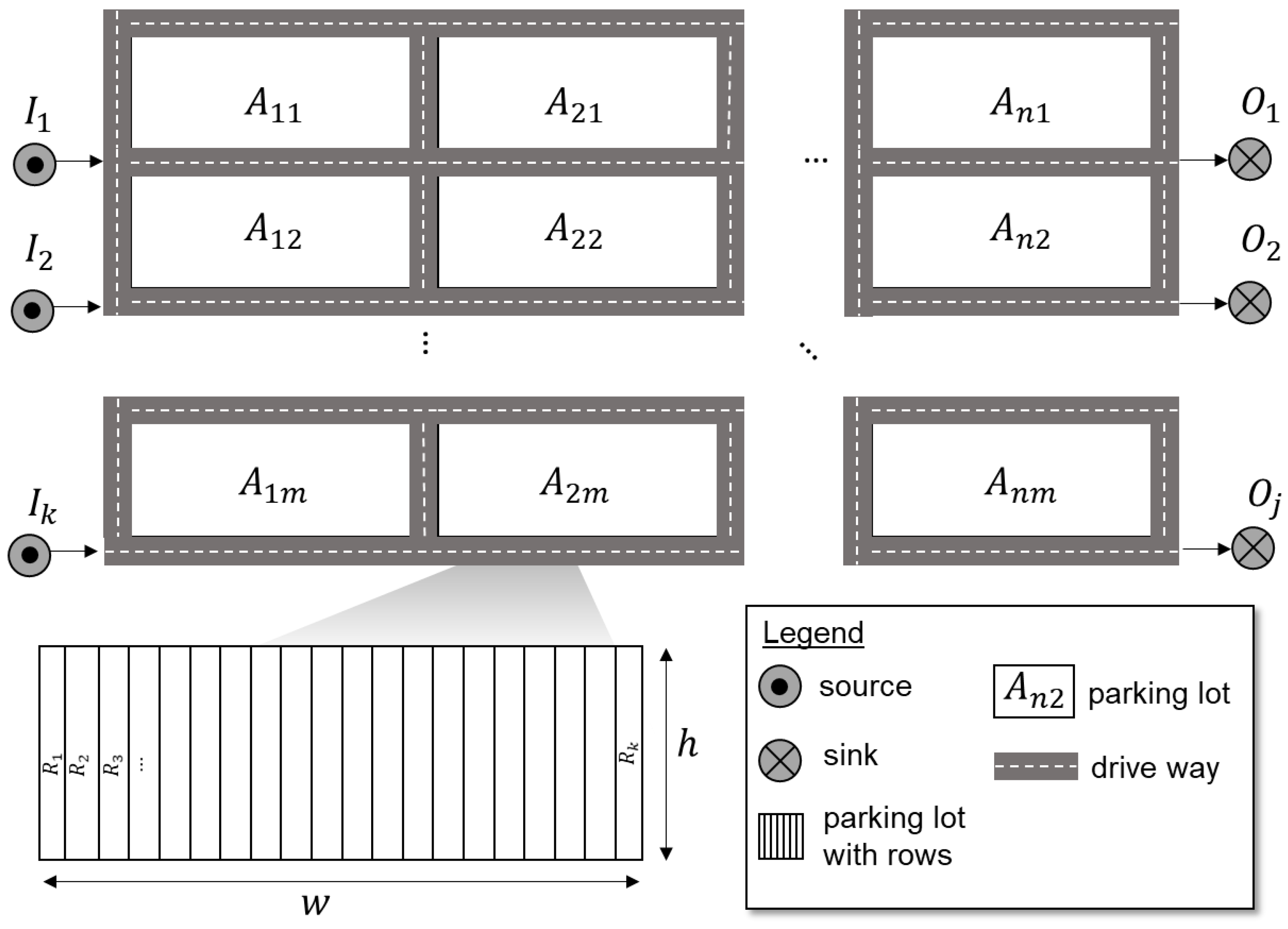
For the basic evaluation in this study, a scalable generic terminal scenario is under consideration (see [12] and [13] for a detailed description) with a specific parameterization described in the following. Figure 2 shows the scalable model, which can be used for analyzing situations of different degrees of structural and dynamic complexity. It consists of parking blocks ( to ) that are interconnected by driveways. Cars arrive at the sources ( to ) and leave the terminal via sinks ( to ). In this context, sources and sinks may represent every carrier (rail, truck, ship). In the case at hand, we focus on a scenario with a layout of 6 × 6 storage areas (blocks). On a more detailed level, each storage block consists of parking rows with a height (), an area width (), and a row width (). These parameters define the capacity of a parking area for cars with a standardized length.
All area parameters are equally set as follows: the area width is , the area height is , and the row width is . This leads to an area capacity of 611 per parking area for cars with a length of 5.1 m. Hence the total capacity in the 6 × 6 scenario is approximately 22,000 (21,996) vehicles.
To keep the model as simple as possible, all vehicles arrive at the terminal via rail and leave it via ship. We assume that in this scenario six OEMs (OEM1 to OME6) ship their cars via this terminal to six different destinations (D1 to D6). As already mentioned, a group of cars is defined as the mix of OEMs, model types and destinations. This is a typical grouping categorization at automobile terminals [8].
To keep the analysis of the generic scenario simple, we assume that there is only one model type per OEM. Hence, we define our groups of vehicles only by OEM and destination. Like in [13], seasonal dynamics of incoming vehicle volumes are modelled by using a sinusoidal arrival function. In this context, each group of cars has a different function regarding the amplitude and the phase shift , while the mean arrival volume () remains constant for all groups. In this context, period determines the seasonal characteristics of this arrival function. The period has be set to a quarter year. The following equation shows the underlying sine function for all groups of cars :
In order to provide a certain level of dynamics, the mean arrival rate, the amplitude and the phase shift are varied systematically. Each OEM-destination combination has a different mean arrival rate (see Table 1). In total, the sum for each OEM is a mean arrival rate of 200 vehicles per day. The mean amplitude is set to 95%. Phase shifts for all destinations of one OEM varied in steps of 20% of a period. The initial inventory of cars per OEM-destination-combination is set to 2000 vehicles. Table 1 summarizes all relevant parameters for incoming cars in this scenario. It should be noted that values in Table 1 may be fractional due the general characteristics of the sine function. For generation of our simulation instances, daily incoming vehicle volumes are rounded to the nearest integer values. The dynamics induced by using the sine function in Equation (1) can be compared to classical seasonal demand fluctuations. This is a typical kind of dynamic, occurring in automobile supply chain.
Outbound processes for cars are modelled ship-wise. There are three groups of ships carrying cars from the terminal model. The following Table 2 shows all relevant parameters for ship arrivals.
The arrival of a ship is uniformly distributed over the simulation period of one year. Each ship carries a certain normally distributed (see Table 2 for expected values and standard deviations) number of cars. In this scenario, a ship may carry vehicles from all OEMs to two destinations (see Table 2). The turnover time of each car depends on the destination and is normally distributed (see Table 1) with a standard deviation of two days. Cars are assigned to ships in a strictly FIFO order. This kind of assignment pre-defines the varying share of destinations and OEMs for a ship.
3.1.2. Evaluation of KPIs for the Generic Model
As depicted in Section 2, terminal planning processes can be evaluated by multiple logistics key performance indicators (KPIs). Especially, efficient process execution and a high productivity play a key role. Thus, this analysis will focus on two typical terminal KPIs. The first KPI is the total driving distance of cars (from the source to the sink). The total driving distance is directly connected to the efficiency of the yard and the berth assignment method. Improved planning results lead to shorter driving distances. This leads consequently to shorter handling times for workers and to a higher productivity.
The second KPI is the degree of sorting. It describes the mixture of cars from different categories in one parking block. In real-world applications, better sorting results lead to less resorting, storage defragmentation and handling processes. Accordingly, a good sorting of cars leads to higher productivity. In our evaluation we focus on the mixture of car groups in the parking block (see Figure 2). It is defined as the ratio between the number of cars of the largest group (e.g., cars from OEM 1 to destination 2) in a parking block and the sum of all cars in the parking block.
3.1.3. Benchmarks Planning Methods
In order to compare the performance of the new methods, the planning tasks (i.e., yard planning and berth planning) described in Section 2 should also be solved by conventional approaches. For yard planning, a simple assignment method has been implemented. For each OEM there are six storage areas exclusively reserved (e.g., OEM1: A11, A21, …, A61, and so on). Within these areas there is for each OEM-destination-combination a certain preferred storage area preassigned. Based on the estimated turnover times and the incoming volumes, destinations with a high turnover time will be located at areas further away from the quayside, and vice versa. This kind of assignment is comparable to a forecast-driven long-term yard plan. We call this method in the following conventional yard planning (CYA).
To have a kind of upper bound, a second method is implemented in terms of a random assignment. Cars entering the terminal choose randomly a parking row in the storage areas associated with the respective OEM. From a benchmark perspective this is obviously the worst kind of assignment. It is expected that it will cause long driving distances and a poor sorting degree. We call this method randomized yard assignment (RYA).
For berth assignments, three different methods are implemented. The first method assigns ships according to the center of gravity for the pre-assigned storage areas coming from the CYA yard method described above. Accordingly, each group of ships has a pre-defined preferred berth and will be assigned to this berth. We call it the following CBP (conventional berth preference-based assignment).
The second, more sophisticated, method calculates driving distances for all associated cars and berths. It assigns a ship to the next unoccupied berth with the shortest route for all cars from the storage area to the berth. This method is like classical berth allocation algorithms (as described in Section 2.1). We call this method the following BAA (berth allocation algorithm) method.
The last method is a random assignment to an unoccupied berth. Like for the yard planning, this method can be seen as an upper bound for the evaluation. We call it random berth allocation (RBA).
3.2. Real-World Scenario
In addition to the described generic terminal model, the evaluation in this paper is based on a real-world terminal case. This section and its subsections describe the real-world terminal, its implementation to a discrete event simulation model, and compares it to the generic scenario describe above. Moreover, it presents the evaluation benchmarks for the analysis of results.
3.2.1. Automobile Terminal Scenario and Simulation Model
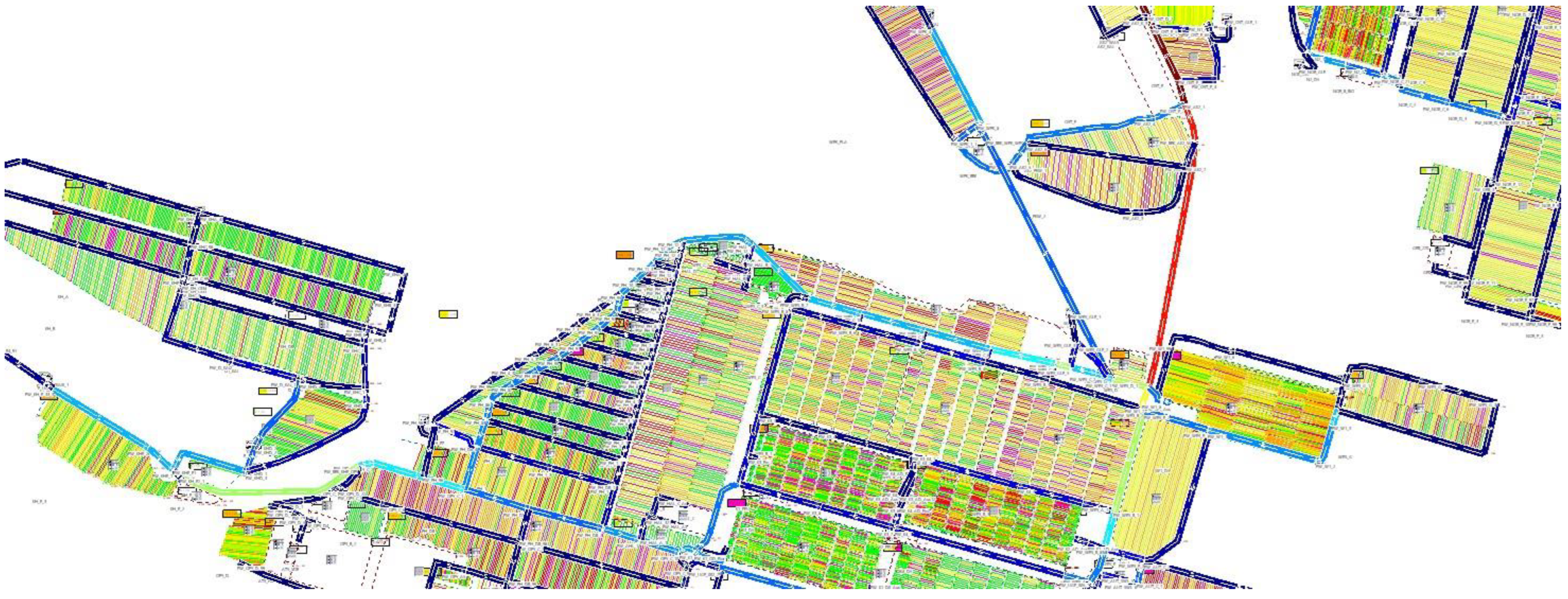
The example terminal is located in Bremerhaven (Germany) and is one of the world’s largest automobile terminals. It has a capacity of approximately 95,000 cars and covers an area of 240 hectares. It comprises 11 different berths and 18 transition points for rail and trucks [35]. The vast majority of parking lots are organized in rows like in the generic scenario. Per year, approximately 1.8 million cars run through this terminal. Both main processes (namely import and export of vehicles) will be addressed in this study. Cars for export mainly arrive via rail and leave the terminal after a relatively short storage period via ship. Import cars arrive via vessel and will be mostly shipped to the local car dealers via truck. Mostly they have a longer turnover time.
Figure 3 shows the implementation of this terminal in a simulation model. Like the generic model, this simulation model comprises all storage areas including all storage rows, rail sidings, and berths. Routes between storage areas and other objects (like e.g., berths) are true to scale in the real world.
The model comprises historical terminal data from 2020 with approximately 1.8 million cars. The grouping of cars is implemented like in the generic model. In the export, there are 71 OEMs with different destinations. In addition, the vehicle model is a further grouping attribute. To sum up, there are 5367 groups for export cars. The situation for import cars is slightly different: there are 1706 groups. To sum up, there are in total k = 7073 groups of cars. Regarding the berth assignment, there are 37 groups of ships sailing to different destinations that can be identified. In total, 1245 ships are included in the simulation study with their lay times and respective berth utilization. Table 3 summarizes the differences between the generic and the real-world scenario. In the evaluation, the mentioned groups are the basis for the pheromone-based yard and berth assignments. Specific rules for trucks and rail assignments are not implemented. Due to the flexibility of trucks, it is assumed that trucks drive directly to the storage areas and start loading autarkically.
The rail arrival points are generally fixed in the long-term planning and cannot be changed during the year. However, similar pheromone-based assignment rules could be easily added for trucks and rails.
3.2.2. Evaluation Benchmark for the Real-World Case
In contrast to the generic scenario, the real terminal scenario evaluation is based on the historical data from 2020. The results of all necessary planning steps (see Figure 1) are included inherently in these data. It can be seen as a general benchmark. However, in the analysis of the new pheromone-based methods, cars move straight through the processes. This means no extra movements (e.g., for storage defragmentation or similar activities) are included. These additional movements are originally comprised in the historic data. To get a fair comparison between the new pheromone-based methods and historic data (called HD in the analysis) with its conventional planning approach, a second benchmark with rectified movements is considered. In this second approach, the centralized planning benchmark mode (CYA in the following) neglects all additional movements (if there were any). Cars in this mode arrive according to the historic data. Afterwards, their first movement to a storage area is conduced. Subsequent movements are skipped until the car leaves the terminal with its final movement. This leads obviously to shorter driving distances, regardless of the methods applied. Thus, this second mode can be interpreted as a kind of lower bound benchmark for the evaluation. The historical data comprise further information about berth and lay times of ships, which are used for the simulation.
3.3. Deriving an Integrated Autonomous Control Method for Automobile Terminals
Based on the inherent shortcomings and the demands for new planning and control methods, this section and its subsections present a new integrated autonomous control approach. It allows autonomous yard assignment decisions of cars (Section 3.3.1) and autonomous berth allocation decisions of ships (Section 3.3.2).
3.3.1. Pheromone-Based Method for Yard Assignment
The basic autonomous control method for the yard assignment is a pheromone-based approach, as proposed by Görges and Freitag, 2019 [12]. It aims at transferring ants’ natural foraging behavior to the yard assigned. While searching for food, ants leave evaporating pheromone trails, marking possible routes to food sources. These trails attract succeeding ants, and they start to follow them. Succeeding ants increase the pheromone concentration and attract further conspecifics. The natural evaporation of pheromones regulates concentration and the number of following ants [36]. This basic concept can be transferred to terminals as follows: vehicles which have to be assigned to yard areas can be seen as intelligent logistics objects that are able to mark suitable parking rows by leaving artificial pheromones coding information about estimated driving distances between sources, parking rows and possible sinks (i.e., berths), as well as information about the sorting degree and the turnover time. Using turnover times may help to minimize driving distances by allocating cars with a high turnover time to storage areas with longer driving distances, and vice versa. Generally, this principle can be compared to the allocation of high-runner products in a classical warehouse [37]. Vehicles looking for assignment decisions read all available artificial pheromone information and decide according to the concentration of pheromones. Based on the suggestion of previous works, the following formula depicts the pheromone concentration calculation scheme (for more details, see also [12,13]):
The variable is called pheromone value of row i. It is calculated for every available parking row i at the terminal and for all k pre-defined groups of cars moving through the terminal. In this context, a group of cars is categorized according to the attribute combinations of OEM, model, and shipping destination.
These groups will further be denoted by the index k. As Equation (2) shows, consists of four terms. Each term addresses different target value. Additionally, each term can be weighted by a factor . Conceptionally, the range of values for is defined in the range between 0 and 1.
The first term aims at balancing the estimated turnover time related to the number of groups (K) and the rank of driving distances related to all available parking areas (F). This term calculates the ranking position of the estimated distance factor divided by the amount of parking areas F and relates it to the ranking of turnover time of remaining categories. In this context is defined as the distance between the most frequently used source of group k, the storage area of the parking row 𝑖 and the most frequently used sink of group k. The parameter is the moving average of the turnover time (days at the terminal) 𝐺 of the vehicles belonging to category 𝑘. It aims at placing cars with longer turnover times to areas with longer driving distances, and vice versa. The values of and are calculated as a moving average over a pre-defined number of cars that made the latest movements in category 𝑘. The parameter represents the evaporation constant of the approach. Like that described by Armbruster et al., a moving average approach is used to model the evaporation process [28].
The second term takes the mixture of different turnover times into account. It rates the duration of stay of the latest car parked in row i () and of the oldest car belonging to category k. It aims to sort cars according to the first-in-first-out (FIFO) principle, since cars are typically shipped in a FIFO sequence. The third term aims to avoid a high degree of storage segmentation of the cars of group k. Therefore, the volume of vehicles of category in the block of row i is set into relation to volume of vehicles belonging to category . The overall estimated driving distance (from the source to the sink) of vehicles belonging to group k is addressed in the last term. It is defined as the ratio between the estimated distance based on the moving average over the last and the maximal possible distance for category regarding all sources, storage areas and sinks.
Cars using this method take all available pheromone values of available parking rows and choose finally the row with the lowest value of . The natural evaporation process is modelled by a moving average over the last cars of a category. In particular, and are determined by using a moving average. In the following evaluation we call this autonomous control method pheromone-based yard assignment (PYA). From a conceptual point of view this pheromone-based approach focuses solely on data and parameters from the past. It breaks the dependencies in the classical cascade planning process depicted in Figure 1. There is no term, in Equation (2), which relates to forecasts or any other future related data. All terms address data from the past (positioning of previous car groups in term 1 and term 4, turnover times in term 2 and the actual split of cars in term 3). Accordingly, this kind of yard assignment is not prone to changes in forecasts or other dynamics. Its actual decisions are only influenced by previous decisions.
3.3.2. Pheromone-Based Method for Berth Assignment
Like the yard assignment, a pheromone-based method can be formulated for the berth assignment. Therefore, all arriving vessels are grouped according to their destination mix. For example, one group of ships serves destinations D1 and D2, and the second group serves D3 and D4. These groups are denoted in the following as l. The idea of the new pheromone-based berth assignment is to allow ships as intelligent logistic objects to choose berth locations according to an artificial pheromone concentration described by the following equation:
It is less complex than the yard assignment. It takes the estimated driving distances of cars being shipped by the respective ship group l into account. New ships arriving calculate the value for the last cars (the index PBA indicates that the value belongs to the pheromone-based berth assignment) at berth i. The ship takes the next unoccupied berth with the lowest value. Through this decision, ships should potentially decide on berth locations with shorter routes for cars. This distance per car comprises the total route of cars at the terminal from the source to the sink. We call this autonomous control method pheromone-based berth assignment (PBA) during the following evaluation study. Like the PYA approach the PBA method refers only to data from the past. Regarding the classical cascade planning process in Figure 1, it breaks the dependencies to previous and succeeding planning task.
The described approach for berth allocation aims at interacting positively with the PYA method as following: As described in 2.2, pheromone-based decisions are more ponderous than pure rational decision. Less volatile berth assignment decisions may help the PYA anticipate future decisions of ship groups and to find shorter routes between sources and sinks (term 1 and term 4 of Equation (2)). This again may help the PBA to make more stable and reliable berth assignments for ship groups.
3.4. Experimental Design
This paper addresses the new proposed methods from two perspectives by using a generic terminal and a real-world terminal scenario. In a first step, it evaluates the general performance of the new methods (i.e., PYA and PBA) systematically to conventional approaches (CYP, RYA, CBP, RBA and BAA) for both scenarios. Subsequently, it investigates the effects of all parameters of the pheromone-based method (i.e., , and ) with a full factorial design (FFD) analysis. The FFD investigate all possible combinations of parameters (factors) on one or more KPIs. A standard FFD expresses the factor values on two levels (high and low) and analyses the main effects of each factor as well as all interactions of factors on the KPIs [38,39]. To conduct an FFD analysis, 2k experiments are necessary for investigating k factors. In the case at hand this leads to 64 different factor combinations (six factors and two factor levels). To reduce the computational efforts, several approaches for the design of experiments (DOE) exist (e.g., factorial designs or Taguchi method), which aim at reducing the number of combinations. Compared to classical one-factor-at-time approaches (OFAT), the DOE aims to reduce the computational efforts on the one hand side and to keep the advantages of a systematic analysis on the other side. Therefore, DOE approaches usually use context-based knowledge about factors in order to reduce the number of factors (e.g., for fractional factorial designs) [40]. However, compared to other DOE approaches, FFD is the most potent tool to get insights into the behavior of the system [41]. Compared to other DOE techniques, like fractional factorial designs, an FFD is conceptionally open to investigate the impact of all factors. The relevance of factors has not been known or assumed before conducting the experiments. Thus, an FFD is very suitable for a complete factor screening [41,42]. In the case at hand the impact of all factors of the new pheromone-based methods (i.e., , and ) are unknown in advance, too. Neglecting factors might cause misleading interpretation of the result. To avoid this an FFD is applied. Due to the relative low number of factors and the accuracy of this approach, this paper uses a 2k FFD and follows the methodical approach introduced by Law, 2017 [43]. It conducts simulation runs for all combinations and calculates the mean main effects and interactions of factors [44].
Table 4 shows an excerpt of the factorial plan with all possible factor levels (−1 low; 1 high) combinations. Furthermore, it shows parameter values which correspond to the factor levels.
Due to the use of random numbers, each experiment has 10 replications. The simulation result for each of the 64 experiment uses the mean KPI values of the 10 simulation runs. The graphical evaluation of the main effects and the interactions between factors are calculated by these mean values for the KPIs (for calculational details see Law, 2017 [43]).
3.5. Simulation Implementation and Validation
Both scenarios were implemented to a discrete event simulation model using the software Technomatix Plant Simulation (version 16.1). Figure 3 presents a screenshot from the implementation of the real-word case in this simulation software. Both model implementations (generic and real-word scenario) only differ in their terminal topology and in the input data used. The implementation of all other methods (e.g., result logging, pheromone-based decision making, etc.) and logical model elements is similar. Accordingly, all verification steps are identical for both scenarios. As proposed by Banks [45] or Gutenschwager [38], all logical elements and source code objects have been intensively checked and analyzed during a stepwise debugging process. For a validation on both implementations an intensive input–output analysis has been made, as proposed by Banks [45]. A comparison of the theoretical model input and output with the observed simulation output shows that all cars defined by the input sine function are generated and simulated correctly in the generic scenario. For the face validity, all realized driving distances in the validation runs are compared to theoretical possible values. No observed driving distances, which are shorter as the shortest possible route or longer than the theoretical maximum distance, were tolerated for the validation.
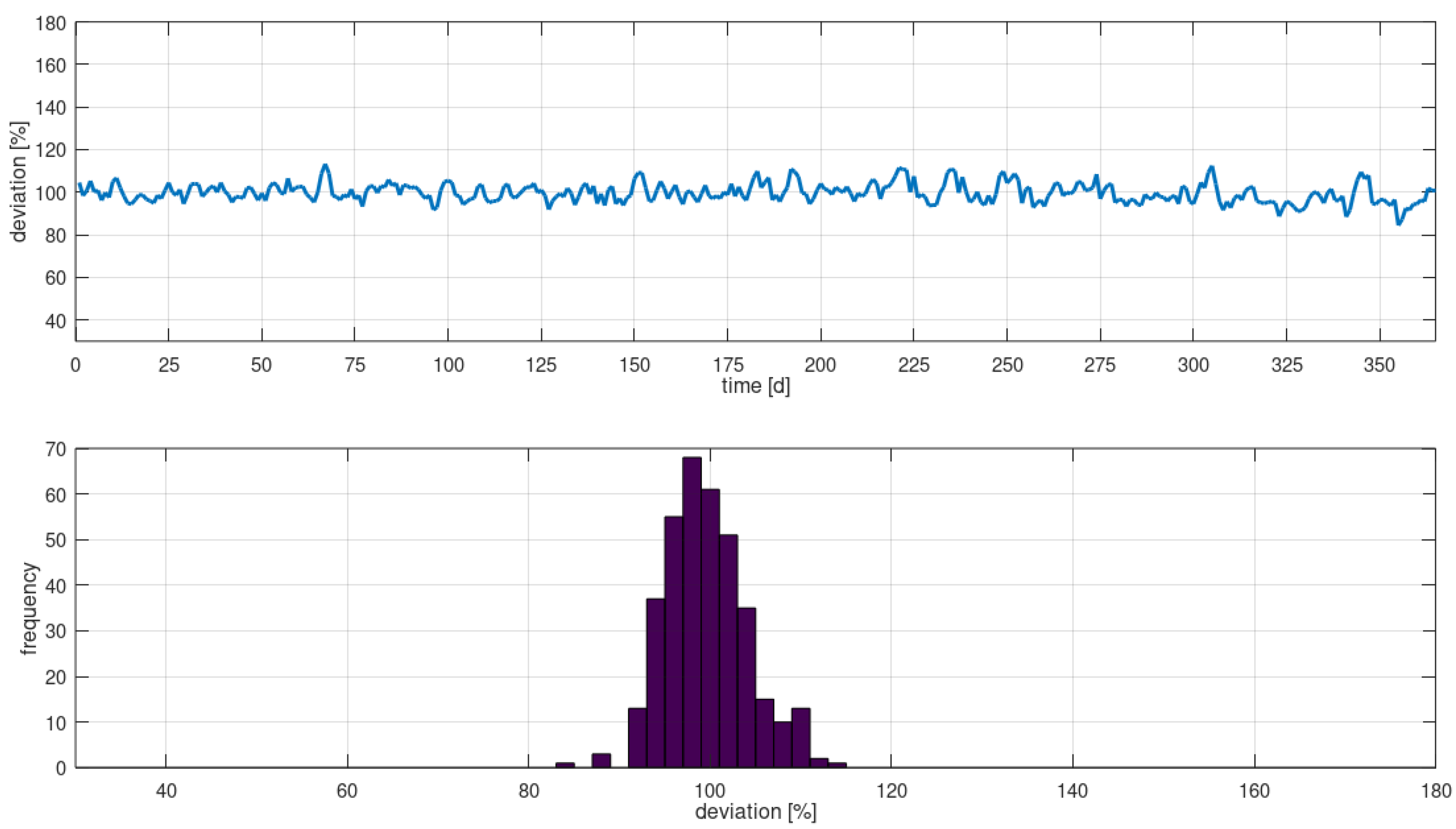
The validation for the real-word case differs. It is based on a comparison of the inventory level in the simulation model and the officially reported daily inventory levels in the terminals yard management system. Figure 4 shows the validation results for the real-world terminal model. It presents the inventory level in the simulation as a ratio of the reported levels. The validation comprises the entire simulation period of one year (i.e., 2020). In Figure 4 there is no deviation between reported and simulated inventory levels if the ratio indicates 100%. If the ratio is below 100%, the inventory level in the simulation is below the reports. If simulated inventory levels were higher than reported values, then the ratio is higher than 100 %.
Figure 4 depicts only moderate deviations in the daily inventory levels. The mean value of the observed deviations for all days is 99.65%. This indicates that there are at least no relevant deviations between the reported daily values and the model. Due to the small observed deviations and the constant distribution of deviations, the model is valid.
4. Results and Discussion
4.1. Performance Evaluation of Generic Scenario
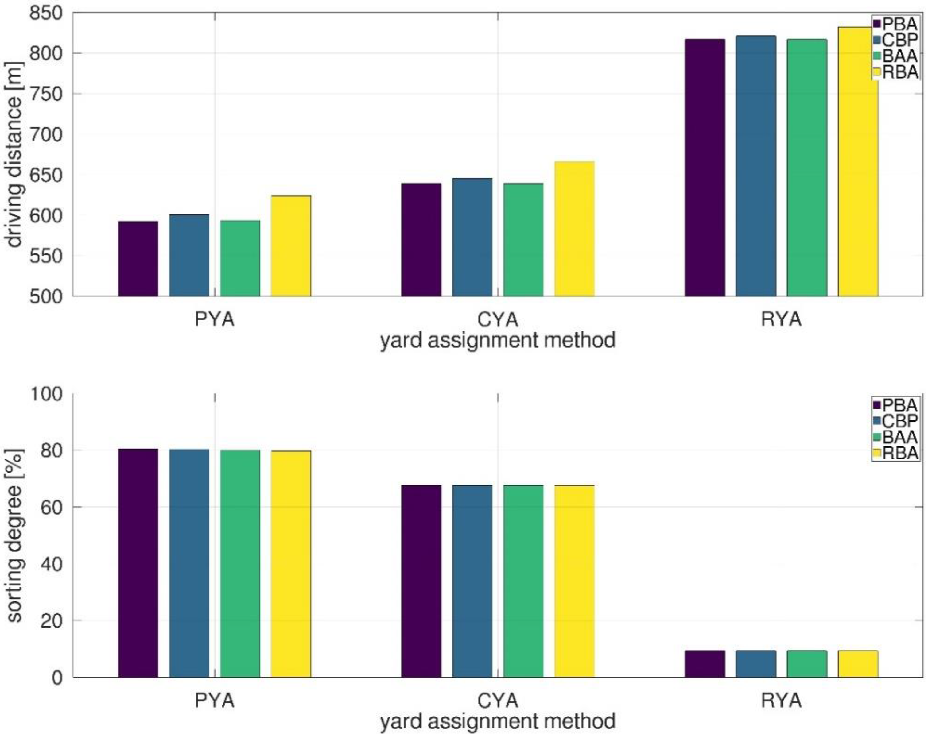
As introduced above, the evaluation focusses in a first step on a comparison between all methods. Every combination of yard and berth planning methods introduced above has been simulated by using the software Technomatix Plant Simulation (version 16.1). Due to the usage of random distributions for the scenario generation, each scenario has been set up 10 times with different random seed values. Accordingly, each combination of allocation methods was simulated 10 times. The following results show the mean values of the respective KPI (total driving distance or sorting result) for the 10 simulation instances. A single run represents a simulation period of one year. In this period, approximately 456,000 cars and 445 ships ran through the system (for details see Table 3). Due to the impact of the evaporation constant of the pheromone-based method (see [12,13]), additional simulation runs for this method have been conducted with varying evaporation constants (for PYA between 800 and 2200; for PBA between 200 and 1400). Hence, this evaluation comprises the results of 1000 simulation runs. For all simulations with the PYA method, we choose the weighting factors as follows: = 0.3, = 0.15, = 0.15, = 0.4. These values led to balanced results for both KPIs in pretesting simulation runs. Figure 5 summarizes the results of the comparison of all combinations of yard and berth allocation methods for both KPIs (total driving distance and sorting degree). In a combination of methods with a pheromone-based method (PYA and PYB), the evaporation constant with the respective best result for this combination is presented.
Figure 5 depicts that a combination of both pheromone-based approaches (PYA-PBA) performs best (591.92 m). However, the combination of PYA-BAA leads to comparable driving distances (593.31 m). The combination of PYA-CBP causes higher mean driving distances (600.43 m). As expected, a random assignment of ships (PYA-RBA) performs worse (623.87 m).
Moreover, Figure 5 shows that all combinations of CYA have longer driving distances than combinations based on the PYA. This indicates that the PYA outperforms the CYA in this setting. However, a combination of the classical yard assignment with a pheromone-based berth assignment may reduce driving distances compared to the combination of both classical assignments (CYA-PBA 638.76 m compared to CYA-CBP 645.34 m). Like the PBA, the BAA leads to comparable results (CYA-BAA 637.73 m). The random-based assignment, which is the upper bound for this evaluation, performs worse. Each combination of a method, the RYA or the RBA, leads to the longest driving times.
A similar result can be observed in the sorting results. All combinations with the PYA lead to the highest sorting degrees. This is an interesting result. As described, it is expected that the CYA leads to good sorting degrees due to its clear assignment to pre-defined parking areas, which will only be violated if there is no free parking space for a particular group. In the case at hand, the utilization of space is temporarily high. Thus, such violation cases may occur during a simulation run and lead the CYA to sorting results below 100%.
Compared to the CYA method, the pheromone-based approach leads to better sorting results. This can be explained by its dynamic character. The PYA reacts more precisely to these temporal overload situations. It directly addresses the sorting degree of cars with terms two and three of Equation (2). As a result, it helps to keep up a good sorting degree.
Furthermore, Figure 5 shows that the impact of the berth assignment method on the sorting degree is low. This can be explained from a conceptual point of view. The allocation of ships to berth takes place after the arrival of cars at the yard, thus it does not affect the sorting of cars.
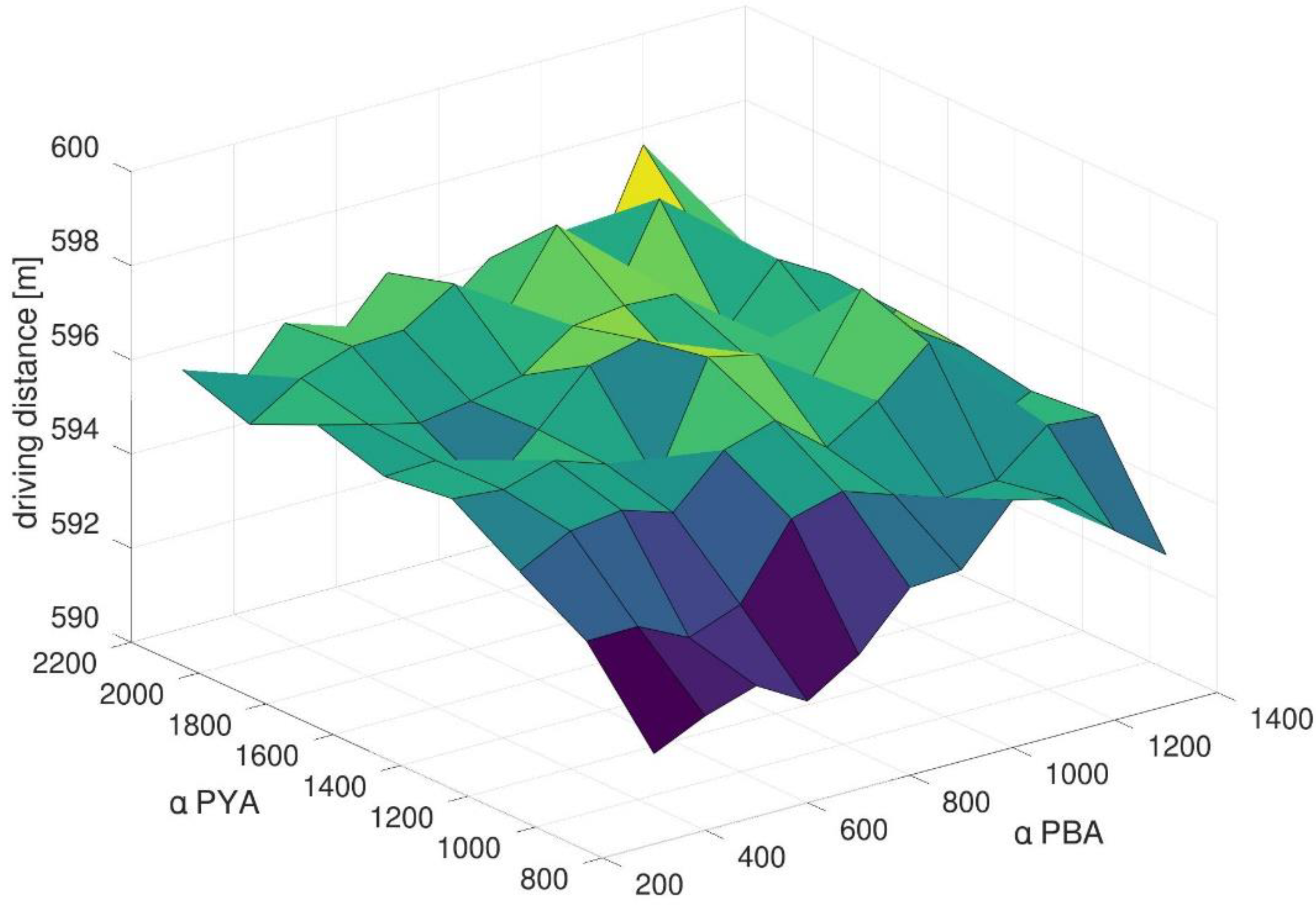
To sum up, Figure 5 shows that combinations of PYA with PBA lead to dominating results regarding sorting degree and total driving distances. However, it does not give information about the impact of the evaporation constants for both methods. Therefore, Figure 6 presents the mean total driving distance for all pheromone-based simulation runs for varying evaporation constants.
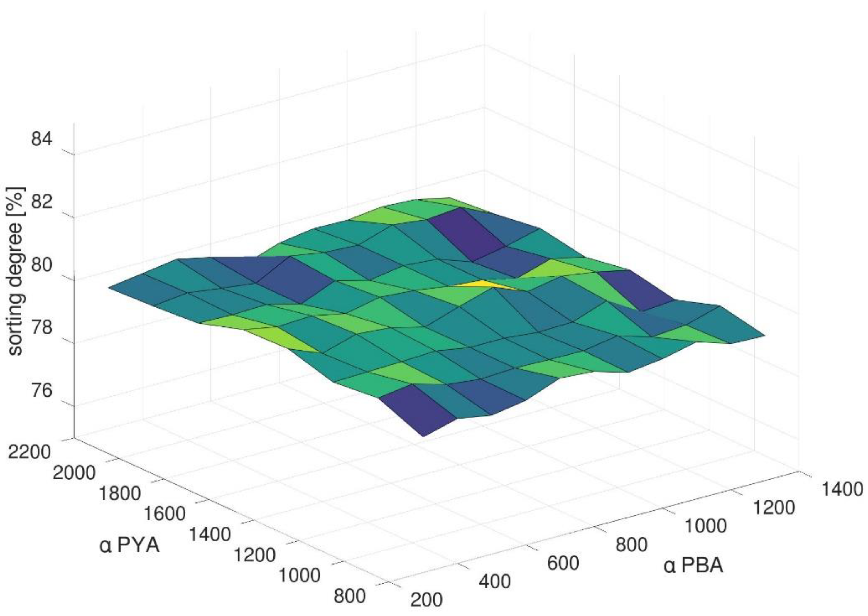
It shows that smaller evaporation constants (both αPYA and αPBA) lead in the case at hand to shorter distances. With smaller evaporation values, the calculation of moving average values in both methods relies on a smaller number of cars. Accordingly, the method can react faster to changing external dynamics. Due to the high dynamics in the arrival and departure rate, the positive effect of smaller evaporation constants seems to dominate. Regarding the sorting degree, Figure 7 shows a different result. For varying evaporation constants, the sorting degree keeps nearly stable. This result can be expected for the berth assignment method (PBA). As described above, all berth allocation methods have conceptually only a small impact on the sorting degree.
This result can be explained by a deeper look in Equation (2). The evaporation constant affects directly terms one and four. As described above, term two addresses the sorting of blocks and rows. Thus, the pheromone value changes directly if there are changes in the sorting. The evaporation constant only affects the sorting result indirectly. A hypothesis in this context may be that this indirect effect of assignment decision does not lead to discernible differences in smaller scenarios with fewer groups of cars. As a result, the sorting degree keeps on a stable level for all simulation runs for combinations of PYA and PBA. We will discuss this hypothesis again during the analysis of the larger real-world scenario.
From a theoretical point of view these results confirm the initial hypothesis, that use of autonomously controlled processes may help to overcome the inherent shortcomings of a centralized planning approach under dynamic conditions. The new pheromone-based yard and berth assignment methods do not need to take any forecast-based information about future system states into account. It can make adequate decisions based only on form the past. The combination of both pheromone-based methods leads to robust and stable local autonomous decisions during the whole simulation period, which results in short driving distances and high sorting degrees.
4.2. Impact of Methods Parameters in the Generic Scenario
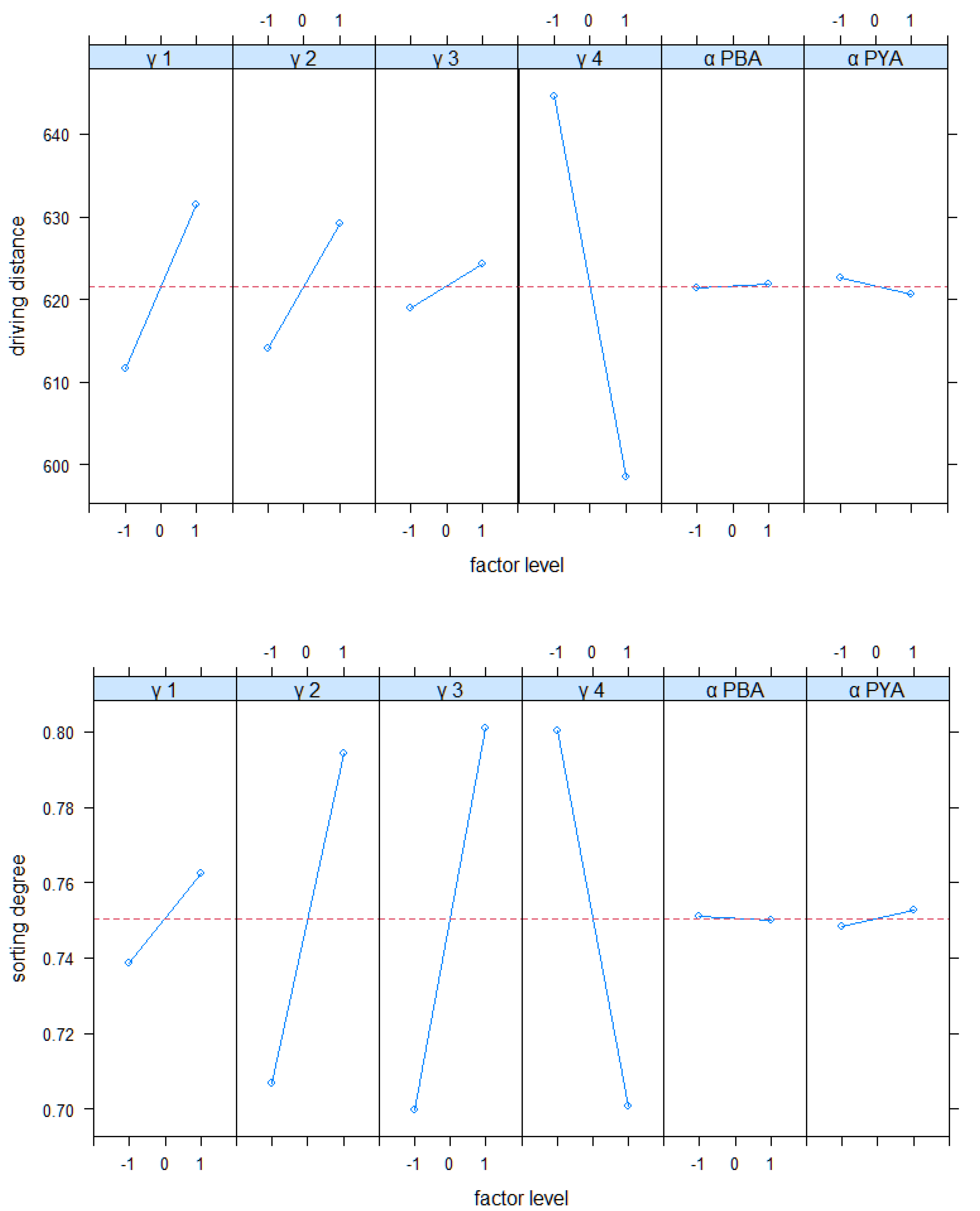
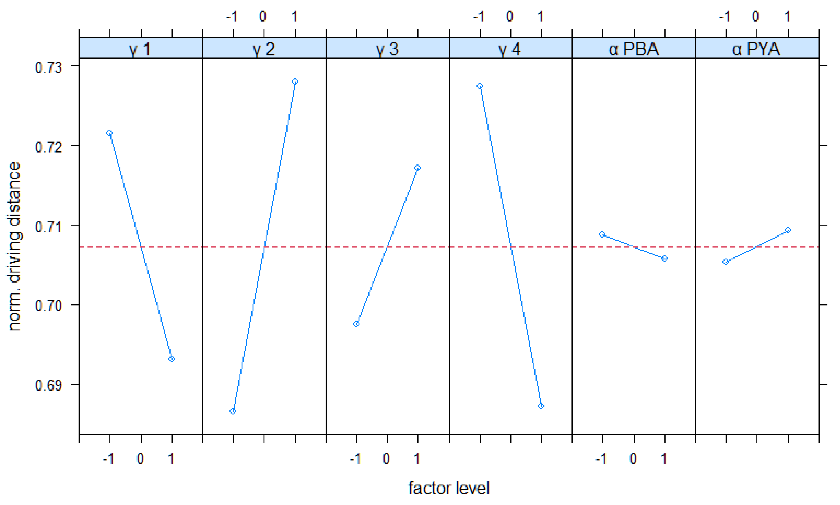
As described in Section 3.1 and Section 3.2, weighing factors and evaporation constants should have a conceptionally planned impact on the terminal’s performance. The first performance evaluation in Section 4.1 confirmed this impact. To get a systematical insight into this effect, we conducted a set of experiments in a full factorial design (see Table 4). Figure 8 shows the results for the main effects of all parameters on the driving distance and the sorting degree.
For the driving distance, the weighting of has the strongest impact. Conceptionally, this factor is directly linked to the driving distance. This result confirms its effectiveness. Regarding factor γ1, the Figure 8 results show an interesting result. It weights the first term of the yard assignment, which comprises the distance as a crucial part. Figure 8 shows that low values lead to short distances and vice versa. Conceptionally, it was expected that a higher weighting decreases the driving distances. This can be explained as follows: a high weighting of this term causes a stronger segmentation of cars with long turnover times. These cars are assigned to areas which are further away from the quayside. The results for the sorting degree confirm this. A high weighting of γ1 seems to cause a stronger segmentation of car groups and better sorting results. In this scenario this effect seems to overrule the originally intended effect. Figure 8 shows that there are effects of the evaporation constant on the driving distance, but it is weaker than the effects of the weighting factors. Especially, the effect of αPBA seems to be neglectable compared to the remaining factors. Regarding the sorting degrees, factors γ2, γ3 and γ4 have the largest effect. As conceptionally planned, γ2 (FIFO) and γ3 (storage segmentation) aim at influencing the sorting of cars. Figure 8 shows that higher weighting of these factors improves the sorting. The factor γ4 has a strong impact on the sorting, too. This can be explained by the greedy nature of term weighted by γ4. It aims at promoting rows with shorter driving distances. For high values rows with shorter distances are preferred, and the sorting is neglected.
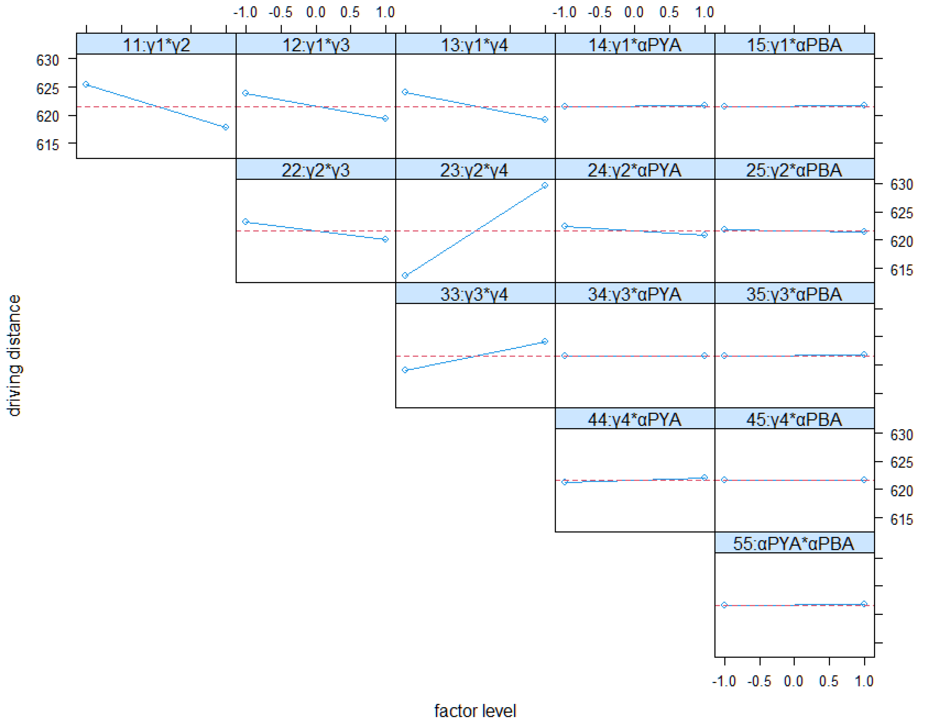
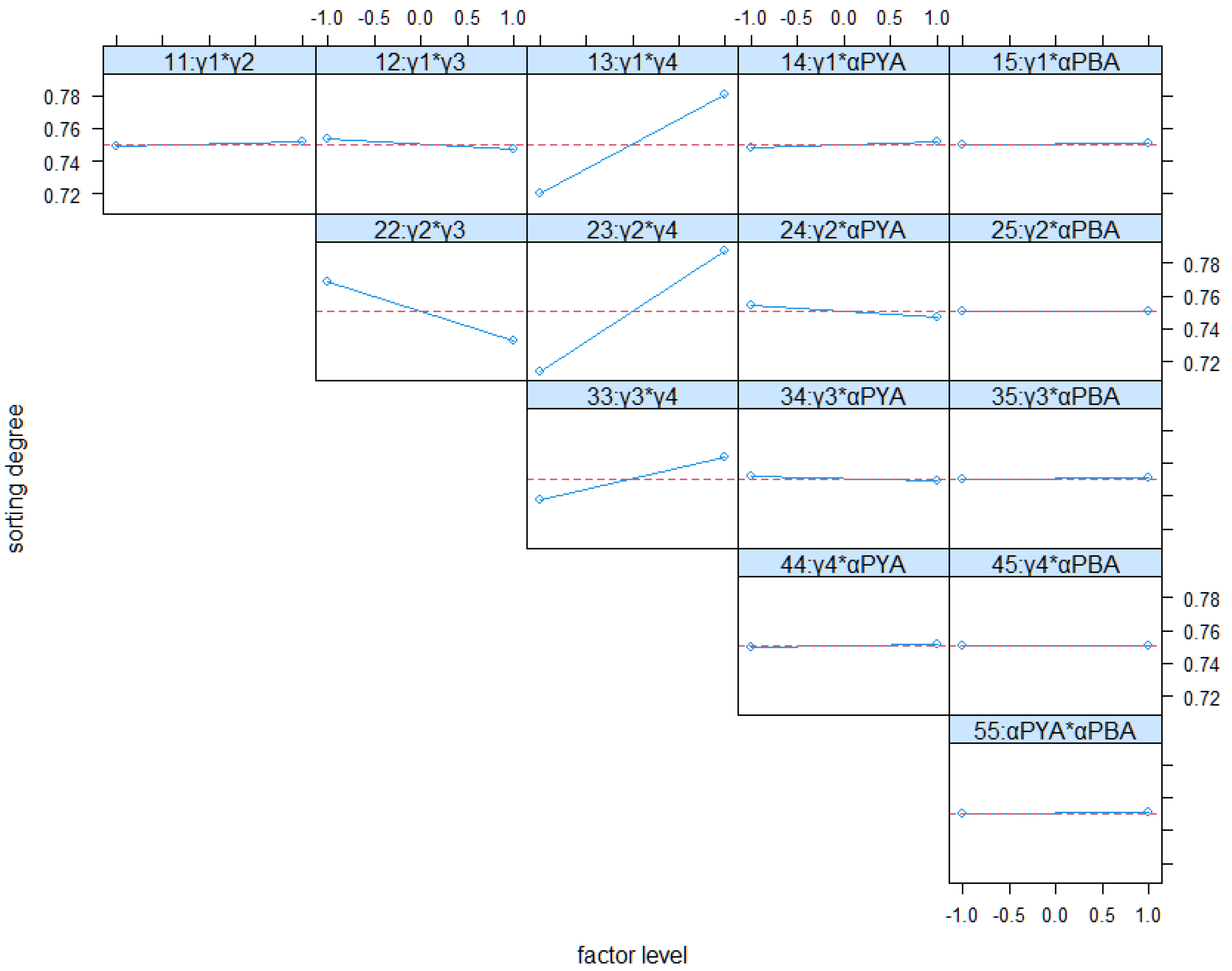
Figure 9 and Figure 10 show the interactions between factors for both KPIs. The interaction between γ2 and γ4 has a strong impact on both KPIs. The interaction between γ1 and γ4 is also of relevance. High weightings of γ1 and γ4 improve both KPIs (short distances and high sorting). This effect is conceptionally desired by differentiating groups according to their turnover times, on the one hand. On the other hand, both factors should help to minimize driving distances, which is confirmed by Figure 9 also.
Other interactions are comparatively low. Especially, interactions between the evaporation constants with the weighting factors seem to have a small impact on both KPIs. In total, the results of the full factorial analysis mainly confirm the conceptional expectations. Only the main effect of γ1 contradicts these expectations.
4.3. Performance Evaluation of Real-Word Scenario
As a first step, the analysis of the generic terminal simulation model showed that both autonomous control methods are theoretically suitable for an auto terminal scenario and may dominate classical planning methods under dynamic conditions. As a next step, the evaluation will focus on a simulation model of a real existing automobile terminal. This section compares the performance of the introduced methods with historical, conventional planned data, to prove the method’s applicability in a real-world case.
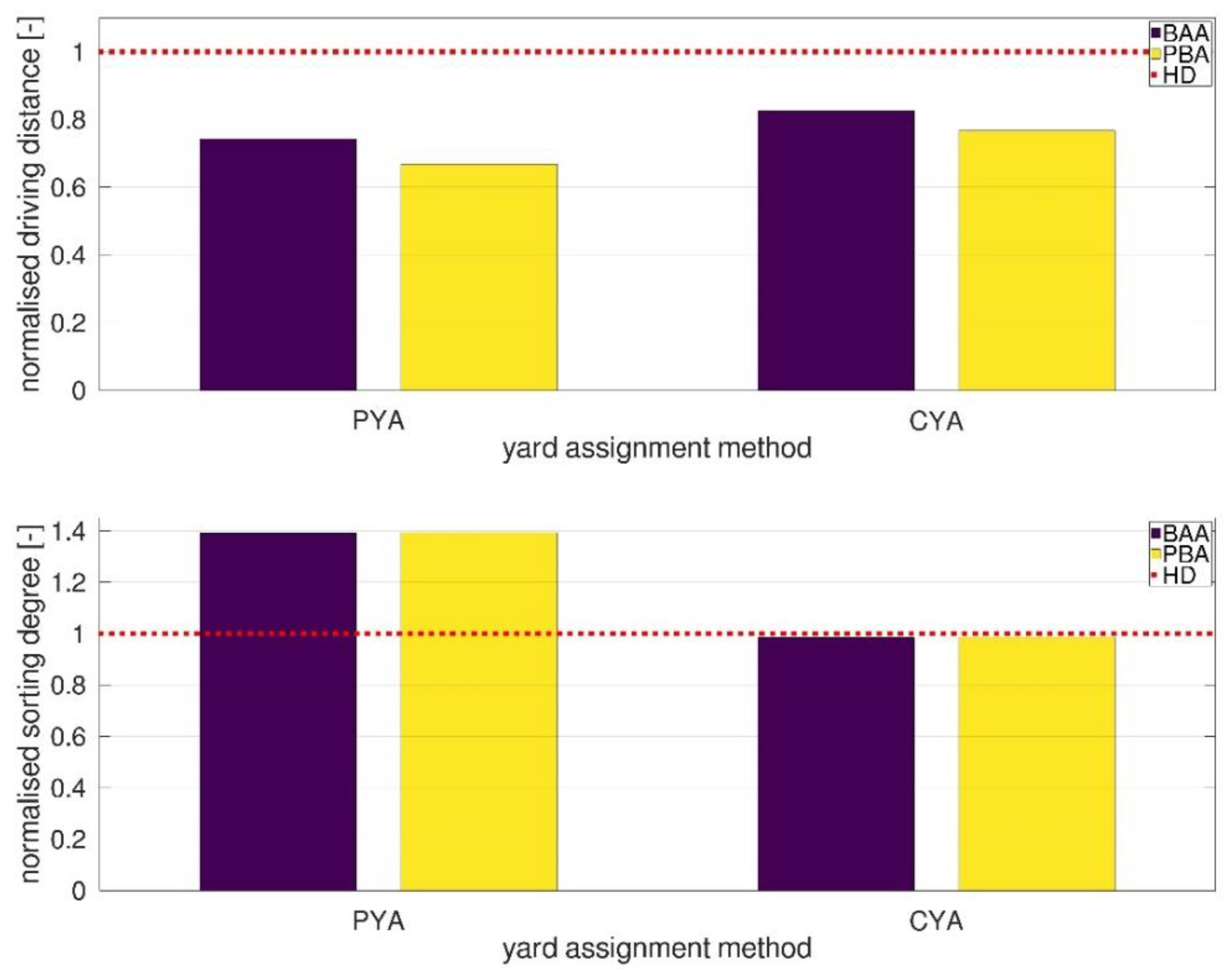
Figure 11 summarizes the simulation results for all the simulation runs with the terminal model of one year. It compares, like Figure 5, the results for all yard assigning methods in combination with the berth assignment methods. It shows un-rectified historic data-based movements (HD), the rectified centralized planning (CYA), and the pheromone-based approach combined with all berth assignment methods (denoted by HD for the historic data assignment, BAA for berth allocation algorithm, PYA and PBA for the pheromone-based assignments). It shows not the absolute values, but its ratio to the main benchmark as a normalization for a better comparison. Accordingly, driving distance results with a normalized ratio smaller than 1.0 have a shorter mean driving distance than the benchmark, and vice versa. The evaluation results for the normalized sorting degree can be seen similarly. Normalized sorting results above 1.0 indicate better sorting compared to the benchmark scenario. As the main benchmark we choose the results obtained with the historic data (HD in the following).
As expected, the HD leads to the longest driving distances. All comparison values are below this benchmark (red dotted line). Compared to the generic scenario, Figure 11 shows a clear difference between the performance of the PBA and the BAA. This can be explained by having a detailed view of the berth utilization, which is quite high in this scenario. Thus, the BAA chooses more often unoccupied berths, with longer total driving distances. This shows that the PBA method can anticipate the berth assignment efficiently in a dynamic scenario with high berth utilization rates. Regarding the results of the PYA combinations, Figure 11 shows the combination PYA-PBA performs best. It leads to the best result with 0.66. The PYA-BAA combination again performs slightly worse (0.74), but better than the CYA-BAA combination (0.82). Comparing PYA-BAA with CYA-PBA (0.76) shows nearly the same results for the driving distance. The dynamic allocation behavior of the PYA method helps to overcome the shortcomings of the BAA in this scenario.
The results of the normalized sorting degree substantiate the findings of the generic model simulation study. As expected, the yard assignment method determines the sorting degree result. In particular, the HD performs slightly better than the CYA (0.98), but the difference is small. In contrast to this, the PYA method performs best and leads to the best sorting degrees. The difference is even bigger than in the generic case. This can be explained by two main effects. The PYA inherently aims at improving the sorting according to the defined groups. It manages the sorting on a row basis, while the centralized approaches take a row and block information into account. A second reason is that the planning HD (and the CYA) focuses on additional sorting criteria for some groups of cars (e.g., grouping of cars for technical treatments). This may overwrite the standard sorting in some cases and lead to deviations in the sorting rules.
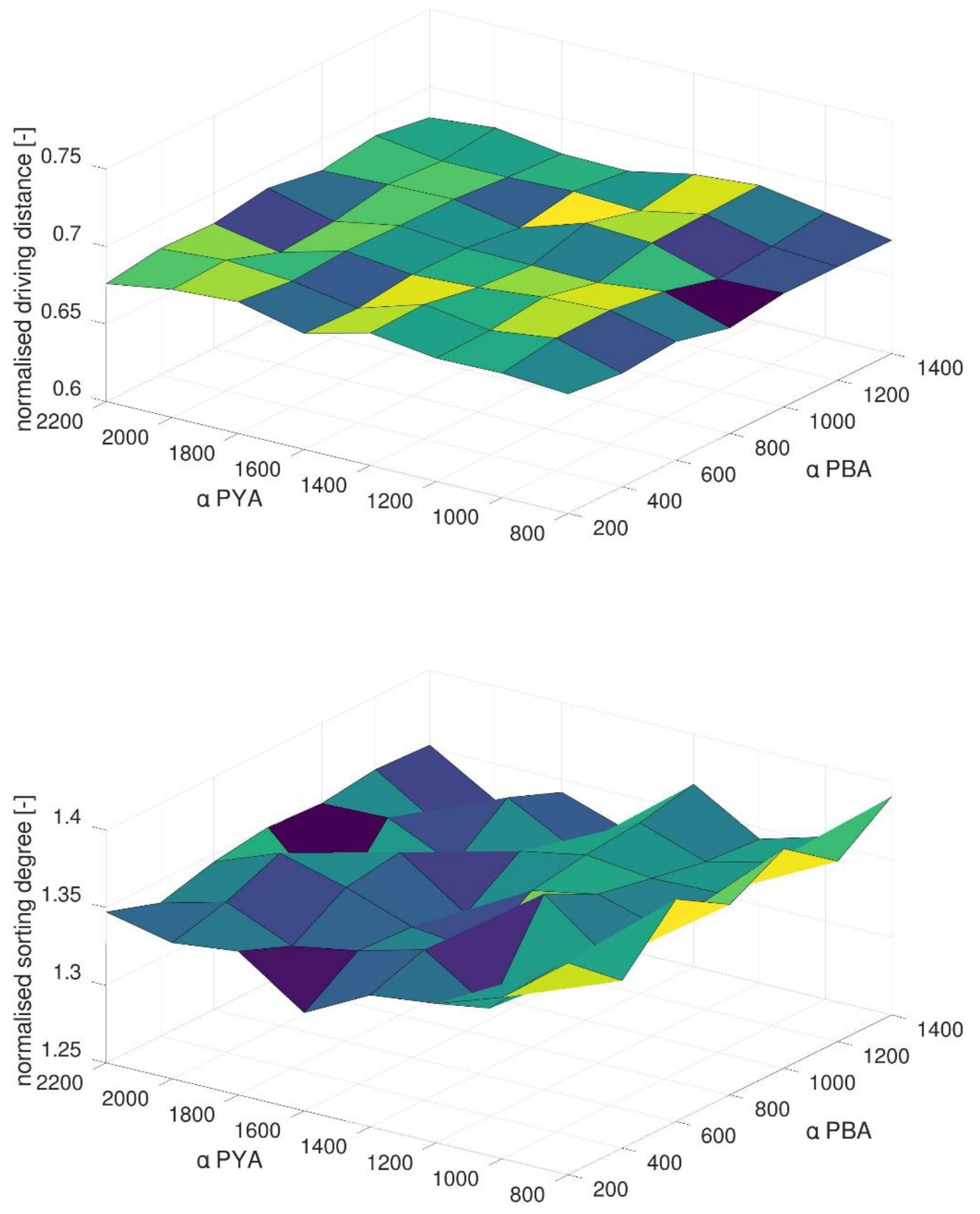
Figure 12 shows the results of the PYP-PBA combinations for varying αPYA and αPBA values. In contrast to the generic scenario, the driving distances in the real terminal model seem not to be sensitive to variations in the evaporation constant.
However, the evaporation constant has an impact on the sorting degree. Figure 12 shows that a better sorting degree can be archived by a smaller αPBA value. In general, this scenario seems to offer more potentials concerning the sorting degree. Compared to the generic scenario, the real case comprises a dramatically higher number of rows and vehicle groups. Consequently, this leads to a higher sorting complexity with more optimization potentials. The PYA method can use these potentials and improve the sorting. However, due to the fact discussed above, both evaporation constants do not have a direct impact due to their equations (Equations (2) and (3)). Thus, this effect seems to be caused indirectly by the dynamics induced by the assignment process. Figure 12 indicates that smaller αPBA values may lead to faster reactions of the method.
These results confirm the findings for the generic scenario concluded in Section 4.1. Each of these autonomous control methods can improve the logistics performance in a real-world scenario. Like in the generic scenario, a combination of both pheromone-based methods leads to the best logistics performance regarding both KPIs. Again, both methods used, as conceptually defined, only use available information about past system states. It does not refer to complex planning processes or any kind of forecast information. These results show that this new approach can provide good and robust decisions in realistic scenarios.
4.4. Full Factorial Analysis of Real-Word Scenario
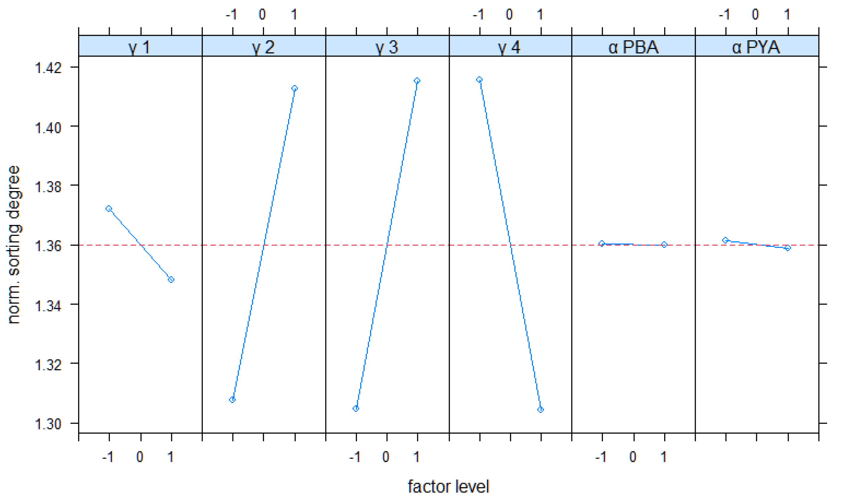
We applied the same full factorial design for a deeper and systematical understanding of all methods parameters in the real-world case. Figure 13 shows the results for the main effects. All observed effects are stronger than in the generic scenario. Except for γ1 and αPBA, all effects are tendentially similar to the observed results in the generic scenario. A significant impact of αPBA can now be observed in this scenario. Higher values of αPBA lead to shorter driving distances. Regarding γ1 these results contradict the observation in the generic scenario. High values of γ1 lead to lower driving distances. A possible explanation is that turnover times in the realistic scenario are more heterogeneous than in the generic scenario. There is still a strong separation of cars with longer turnover times, but it leads in this case to more free storage spaces near the quayside, which can be used by high runner cars. This is the originally intended effect of this parameter. However, this finding indicates that the effect of this parameter is sensitive to the scenario and its configuration.
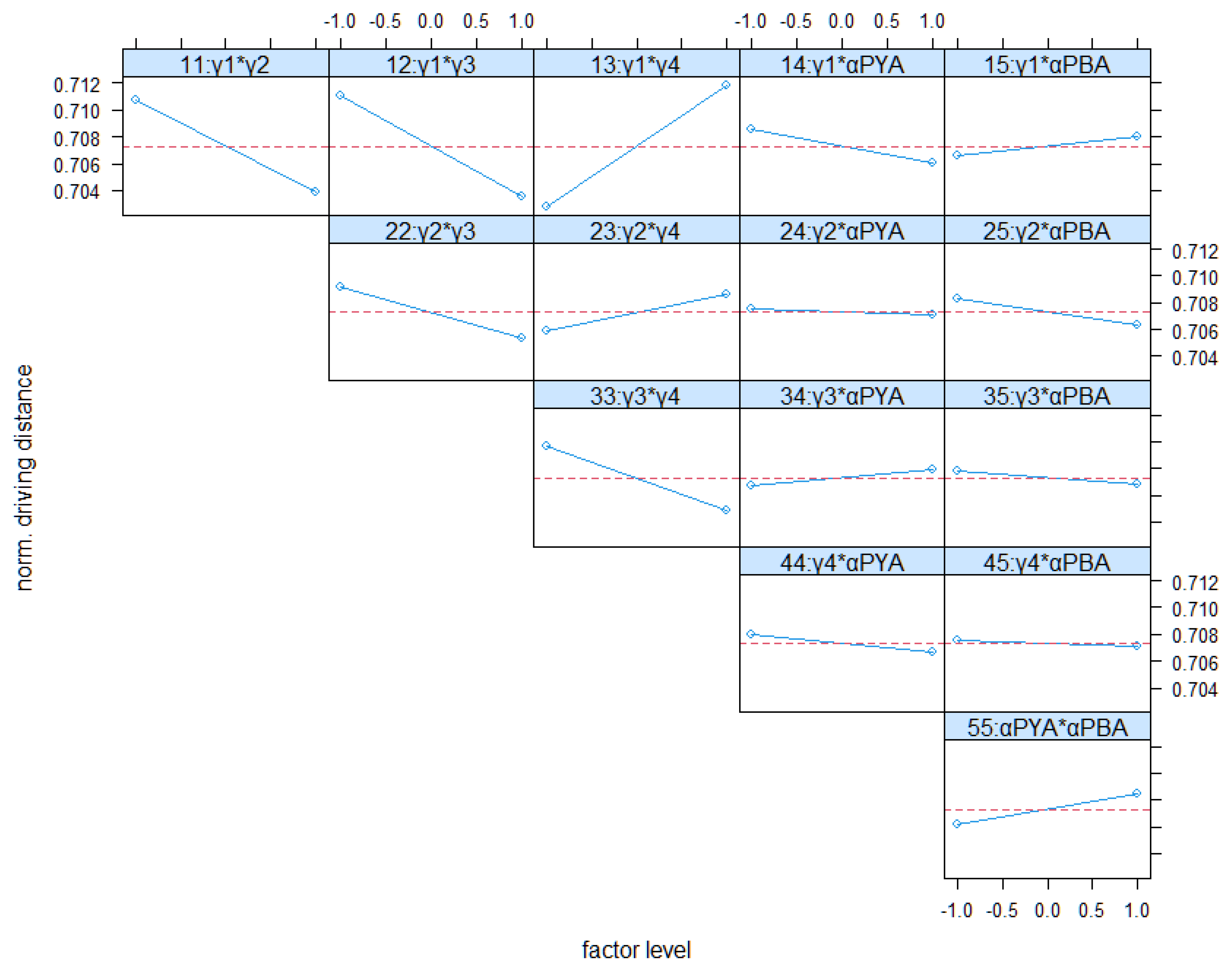
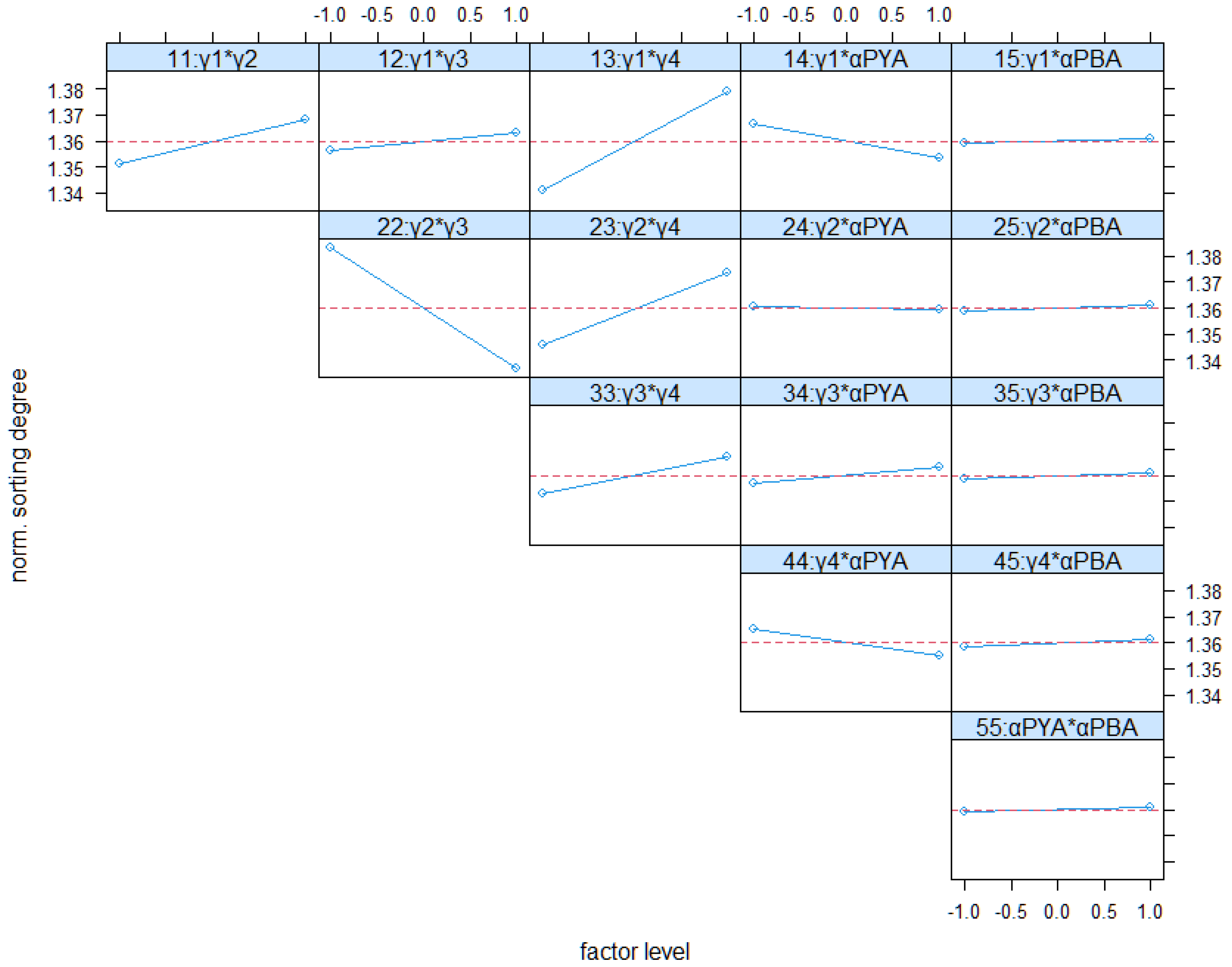
Figure 14 and Figure 15 complete this analysis. They show the interactions of factors on both KPIs, and confirm the observed results from the main effects. In the real scenario all factors and their interactions have a stronger impact on the KPIs, compared to the generic scenario. Especially, γ1 has stronger interactions with the other factors. As already assumed in the discussion of the generic scenario, this can be explained by more heterogeneous turnover times in this real case. The strongest interaction can still be found for factors γ1 and γ4. The impact of interactions between weighting factors and evaporation constants seems to remain low. Both figures confirm this. Only the interaction of γ1 and αPYA has an impact on both KPIs.
To conclude, we can say that the full factorial analysis shows that the weighting factors and the evaporation constant have significant effects on both KPIs. The evaluation shows that all weighting parameters can be used to adjust the logistics performance according to their conceptionally planned purpose. Compared to the generic scenario, the analysis shows that in the real scenario the configuration of all factors becomes more important.
5. Conclusions and Outlook
This paper presented and discussed pheromone-based autonomous control methods to overcome the shortcomings of centralized terminal planning methods for automobile terminals. A discrete event simulation model of a generic automobile terminal scenario has been built to analyze the new approach. This paper showed that both methods (i.e., PYA and PBA) are beneficial under dynamic conditions in this scenario. A combination of the pheromone-based yard assignment and berth allocation leads to the best results observed in this study. Moreover, a full factorial analysis investigated the impact of all methods parameters in depth. It showed that all weighting factors can influence the KPIs in the conceptionally planned manner. In a second step, this paper confirmed these results with a real-world terminal scenario. A real-data-based simulation model of an automobile terminal has been presented. The simulation results confirmed the general findings observed in the generic scenario. A combination of both pheromone-based approaches (yard and berth assignment) performed best in this scenario. An additional full factorial analysis of the real-data-based case confirmed the basic findings from the generic scenario. This new approach seems to be highly suitable to real world applications. Due to its conceptual design this approach can be easily applied to existing terminals. Implementations need no further planning or forecasting information. These pheromone-based approaches can be implemented based on the past data which is usually already available at automobile terminals. However, there are differences in details for some factors which should be investigated in further studies. Especially, the question how to optimize all parameters for specific scenarios seems to be a topic of interest. Another interesting research direction is the refinement of the method by adding additional aspects to the pheromone formulas. This allows addressing further practice-oriented restrictions (e.g., utilization of storage spaces or throughput times).
Author Contributions
Conceptualization, M.G. and M.F.; methodology, M.G. and M.F.; software, M.G.; validation, M.G.; formal analysis, M.G.; investigation, M.G.; resources, M.G. and M.F.; data curation, M.G.; writing—original draft preparation, M.G.; writing—review and editing, M.G. and M.F.; visualization, M.G.; supervision, M.F.; project administration, M.G. and M.F.; funding acquisition, M.G. and M.F. All authors have read and agreed to the published version of the manuscript.
Funding
This research is part of the project “Isabella 2.0—integrated user-oriented control of load movements with artificial intelligence and a virtual training application”, funded by the Federal Ministry for Digital and Transport (BMDV), reference number 19H20001A.
Data Availability Statement
Not applicable.
Conflicts of Interest
The authors declare no conflict of interest.
References
- Nayak, J.; Mishra, M.; Naik, B.; Swapnarekha, H.; Cengiz, K.; Shanmuganathan, V. An Impact Study of COVID-19 on Six Different Industries: Automobile, Energy and Power, Agriculture, Education, Travel and Tourism and Consumer Electronics. Expert Syst. 2021, 39, e12677. [Google Scholar] [CrossRef]
- Esteve-Pérez, J.; Gutiérrez-Romero, J.E.; Mascaraque-Ramírez, C. Performance of the Car Carrier Shipping Sector in the Iberian Peninsula under the COVID-19 Scenario. JMSE 2021, 9, 1295. [Google Scholar] [CrossRef]
- Belhadi, A.; Kamble, S.; Jabbour, C.J.C.; Gunasekaran, A.; Ndubisi, N.O.; Venkatesh, M. Manufacturing and Service Supply Chain Resilience to the COVID-19 Outbreak: Lessons Learned from the Automobile and Airline Industries. Technol. Forecast. Soc. Chang. 2021, 163, 120447. [Google Scholar] [CrossRef]
- Carbone, V.; Martino, M.D. The Changing Role of Ports in Supply-Chain Management: An Empirical Analysis. Marit. Policy Manag. 2003, 30, 305–320. [Google Scholar] [CrossRef]
- Mattfeld, D.C. The Management of Transshipment Terminals: Decision Support for Terminal Operations in Finished Vehicle Supply Chains; Operations Research/Computer Science Interfaces Series; Springer Science + Business Media: New York, NY, USA, 2006; ISBN 978-0-387-30853-1. [Google Scholar]
- Dias, J.C.Q.; Calado, J.M.F.; Mendonça, M.C. The Role of European «ro-Ro» Port Terminals in the Automotive Supply Chain Management. J. Transp. Geogr. 2010, 18, 116–124. [Google Scholar] [CrossRef] [Green Version]
- Görges, M.; Freitag, M. Dynamisierung von Planungsaufgaben Auf Automobilterminals-Potenziale Selbststeuernder Logistischer Prozesse Zur Flexibilisierung Der Flächenmasterplanung. Ind. 4.0 Manag. 2019, 35, 23–26. [Google Scholar]
- Cordeau, J.-F.; Laporte, G.; Moccia, L.; Sorrentino, G. Optimizing Yard Assignment in an Automotive Transshipment Terminal. Eur. J. Oper. Res. 2011, 215, 149–160. [Google Scholar] [CrossRef]
- Dkhil, H.; Diarrassouba, I.; Benmansour, S.; Yassine, A. Modelling and Solving a Berth Allocation Problem in an Automotive Transshipment Terminal. J. Oper. Res. Soc. 2021, 72, 580–593. [Google Scholar] [CrossRef]
- Mattfeld, D.C.; Orth, H. The Allocation of Storage Space for Transshipment in Vehicle Distribution. OR Spectr. 2006, 28, 681–703. [Google Scholar] [CrossRef]
- Böse, F.; Piotrowski, J.; Scholz-Reiter, B. Autonomously Controlled Storage Management in Vehicle Logistics-Applications of RFID and Mobile Computing Systems. Int. J. RF Technol. Res. Appl. 2009, 1, 57–76. [Google Scholar] [CrossRef]
- Görges, M.; Freitag, M. Modeling Autonomously Controlled Automobile Terminal Processes. In Proceedings of the Hamburg International Conference of Logistics (HICL), Hamburg, Germany, 26 September 2019. [Google Scholar]
- Görges, M.; Freitag, M. On the Influence of Structural Complexity on Autonomously Controlled Automobile Terminal Processes. In Dynamics in Logistics; Freitag, M., Haasis, H.-D., Kotzab, H., Pannek, J., Eds.; Lecture Notes in Logistics; Springer International Publishing: Cham, Switzerland, 2020; pp. 42–51. ISBN 978-3-030-44782-3. [Google Scholar]
- Mattfeld, D.C.; Kopfer, H. Terminal Operations Management in Vehicle Transshipment. Transp. Res. Part A Policy Pract. 2003, 37, 435–452. [Google Scholar] [CrossRef]
- Hoff-Hoffmeyer-Zlotnik, M.; Schukraft, S.; Werthmann, D.; Oelker, S.; Freitag, M. Interactive Planning and Control for Finished Vehicle Logistics; epubli: Hamburg, Germany, 2017. [Google Scholar] [CrossRef]
- Beškovnik, B.; Twrdy, E. Managing Maritime Automobile Terminals: An Approach toward Decision-Support Model for Higher Productivity. Int. J. Nav. Archit. Ocean Eng. 2011, 3, 233–241. [Google Scholar] [CrossRef] [Green Version]
- Chen, X.; Li, F.; Jia, B.; Wu, J.; Gao, Z.; Liu, R. Optimizing Storage Location Assignment in an Automotive Ro-Ro Terminal. Transp. Res. Part B Methodol. 2021, 143, 249–281. [Google Scholar] [CrossRef]
- Bierwirth, C.; Meisel, F. A Follow-up Survey of Berth Allocation and Quay Crane Scheduling Problems in Container Terminals. Eur. J. Oper. Res. 2015, 244, 675–689. [Google Scholar] [CrossRef]
- Huang, K.; Suprayogi; Ariantini. A Continuous Berth Template Design Model with Multiple Wharfs. Marit. Policy Manag. 2016, 43, 763–775. [Google Scholar] [CrossRef]
- Lv, X.; Jin, J.G.; Hu, H. Berth Allocation Recovery for Container Transshipment Terminals. Marit. Policy Manag. 2020, 47, 558–574. [Google Scholar] [CrossRef]
- Zhen, L.; Lee, L.H.; Chew, E.P. A Decision Model for Berth Allocation under Uncertainty. Eur. J. Oper. Res. 2011, 212, 54–68. [Google Scholar] [CrossRef]
- Fischer, T.; Gehring, H. Planning Vehicle Transhipment in a Seaport Automobile Terminal Using a Multi-Agent System. Eur. J. Oper. Res. 2005, 166, 726–740. [Google Scholar] [CrossRef]
- Fischer, T.; Gehring, H. Business Process Support in a Seaport Automobile Terminal—A Multi-Agent Based Approach. In Multiagent Based Supply Chain Management; Chaib-draa, B., Müller, J.P., Eds.; Studies in Computational Intelligence; Springer: Berlin/Heidelberg, Germany, 2006; Volume 28, pp. 373–394. ISBN 978-3-540-33875-8. [Google Scholar]
- Olhager, J. The Role of Decoupling Points in Value Chain Management. In Modelling Value; Jodlbauer, H., Olhager, J., Schonberger, R.J., Eds.; Contributions to Management Science; Physica-Verlag HD: Heidelberg, Germany, 2012; pp. 37–47. ISBN 978-3-7908-2746-0. [Google Scholar]
- Wikner, J.; Johansson, E. Inventory Classification Based on Decoupling Points. Prod. Manuf. Res. 2015, 3, 218–235. [Google Scholar] [CrossRef]
- Windt, K.; Böse, F.; Philipp, T. Autonomy in Production Logistics: Identification, Characterisation and Application. Robot. Comput.-Integr. Manuf. 2008, 24, 572–578. [Google Scholar] [CrossRef]
- Windt, K.; Hülsmann, M. Changing Paradigms in Logistics—Understanding the Shift from Conventional Control to Autonomous Cooperation and Control. In Understanding Autonomous Cooperation and Control in Logistics; Hülsmann, M., Windt, K., Eds.; Springer: Berlin/Heidelberg, Germany, 2007; pp. 1–16. ISBN 978-3-540-47449-4. [Google Scholar]
- Armbruster, D.; de Beer, C.; Freitag, M.; Jagalski, T.; Ringhofer, C. Autonomous Control of Production Networks Using a Pheromone Approach. Phys. A Stat. Mech. Its Appl. 2006, 363, 104–114. [Google Scholar] [CrossRef]
- Martins, L.; Varela, M.L.R.; Fernandes, N.O.; Carmo–Silva, S.; Machado, J. Literature Review on Autonomous Production Control Methods. Enterp. Inf. Syst. 2020, 14, 1219–1231. [Google Scholar] [CrossRef]
- Scholz-Reiter, B.; De Beer, C.; Freitag, M.; Jagalski, T. Bio-Inspired and Pheromone-Based Shop-Floor Control. Int. J. Comput. Integr. Manuf. 2008, 21, 201–205. [Google Scholar] [CrossRef]
- Scholz-Reiter, B.; Rekersbrink, H.; Görges, M. Dynamic Flexible Flow Shop Problems—Scheduling Heuristics vs. Autonomous Control. CIRP Ann. 2010, 59, 465–468. [Google Scholar] [CrossRef]
- Rekersbrink, H.; Makuschewitz, T.; Scholz-Reiter, B. A Distributed Routing Concept for Vehicle Routing Problems. Logist. Res. 2009, 1, 45–52. [Google Scholar] [CrossRef]
- Martins, L.M.; Fernandes, N.O.G.; Varela, M.L.R.; Dias, L.M.S.; Pereira, G.A.B.; Silva, S.C. Comparative Study of Autonomous Production Control Methods Using Simulation. Simul. Model. Pract. Theory 2020, 104, 102142. [Google Scholar] [CrossRef]
- Scholz-Reiter, B.; Jagalski, T.; Bendul, J.C. Autonomous Control of a Shop Floor Based on Bee’s Foraging Behaviour. In Dynamics in Logistics; Kreowski, H.-J., Scholz-Reiter, B., Haasis, H.-D., Eds.; Springer: Berlin/Heidelberg, Germany, 2008; pp. 415–423. ISBN 978-3-540-76861-6. [Google Scholar]
- 35. BLG LOGISTICS GROUP AG & Co. KG BLG-AutoTerminal Bremerhaven. Available online: https://www.blg-logistics.com/autoterminal-bremerhaven (accessed on 1 September 2022).
- Van Dyke Parunak, H. “Go to the Ant”: Engineering Principles from Natural Multi-Agent Systems. Ann. Oper. Res. 1997, 75, 69–101. [Google Scholar] [CrossRef]
- Chen, Y.; Li, K.W.; Marc Kilgour, D.; Hipel, K.W. A Case-Based Distance Model for Multiple Criteria ABC Analysis. Comput. Oper. Res. 2008, 35, 776–796. [Google Scholar] [CrossRef]
- Gutenschwager, K.; Rabe, M.; Spieckermann, S.; Wenzel, S. Grundlagen der ereignisdiskreten Simulation. In Simulation in Produktion und Logistik; Springer: Berlin/Heidelberg, Germany, 2017; pp. 51–84. ISBN 978-3-662-55744-0. [Google Scholar]
- Durakovic, B. Design of Experiments Application, Concepts, Examples: State of the Art. Period. Eng. Nat. Sci. 2017, 5, 421–439. [Google Scholar] [CrossRef]
- Czitrom, V. One-Factor-at-a-Time versus Designed Experiments. Am. Stat. 1999, 53, 126. [Google Scholar] [CrossRef]
- Jankovic, A.; Chaudhary, G.; Goia, F. Designing the Design of Experiments (DOE)–An Investigation on the Influence of Different Factorial Designs on the Characterization of Complex Systems. Energy Build. 2021, 250, 111298. [Google Scholar] [CrossRef]
- Law, A.M. Simulation Modeling and Analysis, 5th ed.; McGraw-Hill Series in Industrial Engineering and Management Science; McGraw-Hill Education: Dubuque, IA, USA, 2013; ISBN 978-0-07-340132-4. [Google Scholar]
- Law, A.M. A Tutorial on Design of Experiments for Simulation Modeling. In Proceedings of the 2017 Winter Simulation Conference (WSC), Savannah, GA, USA, 7–10 December 2014; IEEE: Las Vegas, NV, USA, 2017; pp. 550–564. [Google Scholar]
- Guthrie, W.F. NIST/SEMATECH e-Handbook of Statistical Methods (NIST Handbook 151); National Institute of Standards and Technology: Gaithersburg, MD, USA, 2020.
- Banks, J. Discrete-Event System Simulation; Pearson Prentice Hall: Upper Saddle River, NJ, USA, 2005. [Google Scholar]
Figure 1.
Material flow processes and related terminal planning tasks—based on [13].
Figure 1.
Material flow processes and related terminal planning tasks—based on [13].

Figure 2.
Generic automobile terminal scenario [12].
Figure 2.
Generic automobile terminal scenario [12].

Figure 3.
Terminal’s implementation in a simulation model.

Figure 4.
Validation of daily inventory levels.

Figure 5.
Driving distances and sorting degrees for yard and berth methods.

Figure 6.
Impact of evaporation constants on total driving distance.

Figure 7.
Impact of evaporation constants on sorting degree.

Figure 8.
Main effects of FFD study in the generic scenario.

Figure 9.
Factor interactions for driving distance in the generic scenario.

Figure 10.
Factor interactions for sorting degree in the generic scenario.

Figure 11.
Normalized driving distances and sorting degrees for yard and berth methods.

Figure 12.
Impact of evaporation constants on normalized terminal KPIs.

Figure 13.
Main effects of FFD study in the real-data-based model.


Figure 14.
Factor interactions on norm. Driving distance in the real-data-based model.

Figure 15.
Interactions on norm. Sorting degree in the real-data-based model.


Table 1.
Arrival parameters in the generic model.
| OEM | Destination | Ship Group | Avg. Arrival Rate [Cars/Day] | Amplitude [Cars/Day] | Relative Phase Shift [−] | Avg. Turnover Time [d] |
|---|---|---|---|---|---|---|
| OEM 1 | D1 | R3 | 47.62 | 45.24 | 0 | 10 |
| D2 | R3 | 38.10 | 36.20 | 0.2 | 15 | |
| D3 | R2 | 28.57 | 27.14 | 0.4 | 20 | |
| D4 | R2 | 19.05 | 18.10 | 0.6 | 25 | |
| D5 | R1 | 9.52 | 9.04 | 0.8 | 30 | |
| D6 | R1 | 57.14 | 54.28 | 1 | 5 | |
| OEM 2 | D1 | R3 | 38.10 | 36.20 | 0 | 15 |
| D2 | R3 | 28.57 | 27.14 | 0.2 | 20 | |
| D3 | R2 | 19.05 | 18.10 | 0.4 | 25 | |
| D4 | R2 | 9.52 | 9.04 | 0.6 | 30 | |
| D5 | R1 | 57.14 | 54.28 | 0.8 | 5 | |
| D6 | R1 | 47.62 | 45.24 | 1 | 10 | |
| OEM 3 | D1 | R3 | 28.57 | 27.14 | 0 | 20 |
| D2 | R3 | 19.05 | 18.10 | 0.2 | 25 | |
| D3 | R2 | 9.52 | 9.04 | 0.4 | 30 | |
| D4 | R2 | 57.14 | 54.28 | 0.6 | 5 | |
| D5 | R1 | 47.62 | 45.24 | 0.8 | 10 | |
| D6 | R1 | 38.10 | 36.20 | 1 | 15 | |
| OEM 4 | D1 | R3 | 19.05 | 18.10 | 0 | 25 |
| D2 | R3 | 9.52 | 9.04 | 0.2 | 30 | |
| D3 | R2 | 57.14 | 54.28 | 0.4 | 5 | |
| D4 | R2 | 47.62 | 45.24 | 0.6 | 10 | |
| D5 | R1 | 38.10 | 36.20 | 0.8 | 15 | |
| D6 | R1 | 28.57 | 27.14 | 1 | 20 | |
| OEM 5 | D1 | R3 | 9.52 | 9.04 | 0 | 30 |
| D2 | R3 | 57.14 | 54.28 | 0.2 | 5 | |
| D3 | R2 | 47.62 | 45.24 | 0.4 | 10 | |
| D4 | R2 | 38.10 | 36.20 | 0.6 | 15 | |
| D5 | R1 | 28.57 | 27.14 | 0.8 | 20 | |
| D6 | R1 | 19.05 | 18.10 | 1 | 25 | |
| OEM 6 | D1 | R3 | 57.14 | 54.28 | 0 | 5 |
| D2 | R3 | 47.62 | 45.24 | 0.2 | 10 | |
| D3 | R2 | 38.10 | 36.20 | 0.4 | 15 | |
| D4 | R2 | 28.57 | 27.14 | 0.6 | 20 | |
| D5 | R1 | 19.05 | 18.10 | 0.8 | 25 | |
| D6 | R1 | 9.52 | 9.04 | 1 | 30 |
Table 2.
Parameters of ships arriving in the generic scenario.
| Ship Group | Avg. Number of Cars per Journey | Standard Deviation | Destinations |
|---|---|---|---|
| R1 | 1000 | 150 | D5, D6 |
| R2 | 1000 | 150 | D3, D4 |
| R3 | 1000 | 150 | D1, D2 |
Table 3.
Comparison of the generic and real-world scenario.
| Generic Scenario | Real-World Scenario | |
|---|---|---|
| Annual volume | 456,202 | 1,765,787 |
| Number of parking rows | 1692 | 18,825 |
| Terminal capacity | 21,996 | 104,478 |
| Annual ship arrivals | 447 | 1245 |
| Groups of cars | 36 | 7073 |
| Number berth | 5 | 11 |
Table 4.
Excerpt of the full factorial plan.
| Parameter Value | Factor Level | ||||||||||||
|---|---|---|---|---|---|---|---|---|---|---|---|---|---|
| # | Runs | γ1 | γ2 | γ3 | γ4 | αf | αs | γ1 | γ2 | γ3 | γ4 | αf | αs |
| 1 | 10 | 0.05 | 0.05 | 0.05 | 0.05 | 500 | 200 | −1 | −1 | −1 | −1 | −1 | −1 |
| 2 | 10 | 0.95 | 0.05 | 0.05 | 0.05 | 500 | 200 | 1 | −1 | −1 | −1 | −1 | −1 |
| 3 | 10 | 0.05 | 0.95 | 0.05 | 0.05 | 500 | 200 | −1 | 1 | −1 | −1 | −1 | −1 |
| 4 | 10 | 0.95 | 0.95 | 0.05 | 0.05 | 500 | 200 | 1 | 1 | −1 | −1 | −1 | −1 |
| 5 | 10 | 0.05 | 0.05 | 0.95 | 0.05 | 500 | 200 | −1 | −1 | 1 | −1 | −1 | −1 |
| 6 | 10 | 0.95 | 0.05 | 0.95 | 0.05 | 500 | 200 | 1 | −1 | 1 | −1 | −1 | −1 |
| 7 | 10 | 0.05 | 0.95 | 0.95 | 0.05 | 500 | 200 | −1 | 1 | 1 | −1 | −1 | −1 |
| 8 | 10 | 0.95 | 0.95 | 0.95 | 0.05 | 500 | 200 | 1 | 1 | 1 | −1 | −1 | −1 |
| 9 | 10 | 0.05 | 0.05 | 0.05 | 0.95 | 500 | 200 | −1 | −1 | −1 | 1 | −1 | −1 |
| 10 | 10 | 0.95 | 0.05 | 0.05 | 0.95 | 500 | 200 | 1 | −1 | −1 | 1 | −1 | −1 |
| 11 | 10 | 0.05 | 0.95 | 0.05 | 0.95 | 500 | 200 | −1 | 1 | −1 | 1 | −1 | −1 |
| 12 | 10 | 0.95 | 0.95 | 0.05 | 0.95 | 500 | 200 | 1 | 1 | −1 | 1 | −1 | −1 |
| 13 | 10 | 0.05 | 0.05 | 0.95 | 0.95 | 500 | 200 | −1 | −1 | 1 | 1 | −1 | −1 |
| 14 | 10 | 0.95 | 0.05 | 0.95 | 0.95 | 500 | 200 | 1 | −1 | 1 | 1 | −1 | −1 |
| 15 | 10 | 0.05 | 0.95 | 0.95 | 0.95 | 500 | 200 | −1 | 1 | 1 | 1 | −1 | −1 |
| 16 | 10 | 0.95 | 0.95 | 0.95 | 0.95 | 500 | 200 | 1 | 1 | 1 | 1 | −1 | −1 |
| 17 | 10 | 0.05 | 0.05 | 0.05 | 0.05 | 2500 | 200 | −1 | −1 | −1 | −1 | 1 | −1 |
| … | |||||||||||||
| 64 | 10 | 0.95 | 0.95 | 0.95 | 0.95 | 2500 | 1500 | 1 | 1 | 1 | 1 | 1 | 1 |
Publisher’s Note: MDPI stays neutral with regard to jurisdictional claims in published maps and institutional affiliations. |
© 2022 by the authors. Licensee MDPI, Basel, Switzerland. This article is an open access article distributed under the terms and conditions of the Creative Commons Attribution (CC BY) license (https://creativecommons.org/licenses/by/4.0/).
Share and Cite
MDPI and ACS Style
Görges, M.; Freitag, M. Design and Evaluation of an Integrated Autonomous Control Method for Automobile Terminals. Logistics 2022, 6, 73. https://0-doi-org.brum.beds.ac.uk/10.3390/logistics6040073
AMA Style
Görges M, Freitag M. Design and Evaluation of an Integrated Autonomous Control Method for Automobile Terminals. Logistics. 2022; 6(4):73. https://0-doi-org.brum.beds.ac.uk/10.3390/logistics6040073
Chicago/Turabian StyleGörges, Michael, and Michael Freitag. 2022. "Design and Evaluation of an Integrated Autonomous Control Method for Automobile Terminals" Logistics 6, no. 4: 73. https://0-doi-org.brum.beds.ac.uk/10.3390/logistics6040073