Integrated Scheduling of Automated Yard Cranes and Automated Guided Vehicles with Limited Buffer Capacity of Dual-Trolley Quay Cranes in Automated Container Terminals

Abstract

Background: The key performance index for the container terminals is the vessel berthing time which is highly affected by the scheduling of the different handling equipment. Proper integrated scheduling of the handling equipment is crucial, especially in automated container terminals, where all the handling equipment is automated and must be coordinated to avoid interference. One of the most challenging problems both scholars and terminal operators face is introducing a proper scheduling plan for different equipment, considering the buffer capacity of dual-trolley quay cranes (QCs) and the limited storage locations of import containers. Methods: A mathematical model is proposed to integrate the scheduling of automated yard cranes and automated guided vehicles (AGVs), considering the limited buffer capacity beneath dual-trolley QCs and the storage allocation of import containers. Results: different instances were solved to evaluate the proposed model’s performance and investigate the impact of using dual-trolley QCs instead of single-trolley QCs, and the impact of using different buffer capacities. Conclusions: The results show that the model provides detailed scheduling and assigning plans for the YCs and AGVs besides allocating import containers. Additionally, the dual-trolley QCs can significantly decrease the completion time and increase AGVs’ utilization compared to the single-trolley QCs.

1. Introduction

Maritime container terminals play a vital role in global trade, as about 80% of global trade is carried by sea [1]. Consequently, there is an ongoing development in the terminals to efficiently serve as many containers as possible at a reasonable time and cost [2]. Terminals started to apply new technologies to serve large-scale operations and increase terminal performance [3]. Automated container terminals (ACTs) are the future as they increase the performance of the terminals and reduce the operational costs of different equipment such as; quay cranes (QCs), yard cranes (YCs), and automated vehicles [4]. In ACTs, each piece of equipment is controlled automatically rather than manually, as in conventional terminals. Moreover, QCs are the most expensive equipment in the terminal, so there is a further improvement on this piece of equipment. Two types of QCs are typically used in ACTs: a single-trolley QC or a dual-trolley QC, as shown in Figure 1a,b. The main difference between them is that the former has one trolley that handles the operations of both vessels and vehicles. While the latter has two trolleys, the main trolley interacts with the vessel, the portal trolley interacts with the vehicles, and there is a buffer beneath each crane. The main benefit of this configuration is to increase the efficiency of the QC and decouple seaside operations from yard-side operations. This research compares the performance of the two types of QCs within an integrated equipment scheduling framework.

Furthermore, two common types of vehicles serve the QCs: automated lifting vehicles (ALVs) and automated guided vehicles (AGVs). ALVs can lift and release containers without assistance from any other equipment. In contrast, AGVs do not have the lifting ability; they operate with the help of QCs or YCs to function. Yu et al. 2022, stated that fifteen out of thirty-nine ACTs worldwide used dual-trolley QCs instead of single-trolley QCs [5]. Nine of them used AGVs, while only three terminals considered ALVs. The remaining terminals used conventional internal trucks [5]. Therefore, this study considers AGVs commonly used with dual-trolley QCs.

However, the container terminal’s most important performance measure is the vessel berthing time, which depends mainly on the completion time of the last job [6,7,8]. The lower the vessel berthing time results in a better terminal performance [9]. The container terminals aim to minimize the vessel berthing time because if the operations on the vessel finish after the expected finishing time, there would be a delay cost per unit time and a penalty cost if the vessel departed after the latest finishing time [10,11,12,13]. On the other hand, the vessel’s berthing time is directly affected by the loading and unloading operations of export and import containers which YCs perform at the yard side or by QCs at the seaside [14].

Furthermore, in ACTs, all equipment is controlled automatically. The interference between each pair of equipment should be determined precisely to avoid any disruption or backlog of cargo [15]. Therefore, integrated scheduling of container terminal handling equipment (i.e., YCs, and AGVs) is one of the most effective ways to increase the performance of a container terminal and the utilization of its handling equipment [2]. Moreover, studying import containers is more complicated than export containers, as it requires arrangement between the scheduling and the assignment of all equipment, besides the availability of storage locations in the storage yard. In addition, considering the buffer capacity beneath QCs is challenging because of its complexity.

Therefore, this article introduces a novel mixed integer programming (MIP) model to integrate the scheduling of AGVs and YCs considering the limited buffer capacity beneath dual-trolley QCs, and the assignment of yard locations to import containers to minimize the vessel berthing time. The rest of this article is organized as follows: Section 2 contains a literature review, Section 3 presents the problem description and model formulation, and Section 4 includes the numerical experiments and results. Finally, Section 5 summarizes the conclusion and future work.

2. Literature Review

Automated container terminals require a higher management level than conventional terminals, as all the equipment is unmanned and needs detailed and regular scheduling to prevent interference [4]. Integrated scheduling has been proven to be very effective in improving the performance of conventional CTs [16,17]. In ACTs, integrated equipment scheduling is a mandatory function to guarantee the smooth operation of the terminal. Therefore, in the literature, we focused only on the integrated problems in ACTs. Based on the available literature, the integrated scheduling problems in ACTs can be divided into two main categories: integrated scheduling considering single-trolley QCs and integrated scheduling considering dual-trolley QCs.

For the first category; Sadeghian et al. integrated the QCs and ALVs scheduling by introducing a mathematical model. The buffer spaces beneath QCs were assumed to be unlimited in their model [18]. Kress et al. introduced a mathematical model to integrate QC and straddle carrier (SCs) scheduling and to solve the routing problem of the SCs [19]. SCs operate similarly to ALVs, with the ability to store containers at the storage yard. They focused on assigning and scheduling SCs, assuming that QC scheduling is known in advance. Castilla-Rodríguez et al. used the simulation–optimization approach to integrate the scheduling of QCs and AGVs to increase the efficiency of the trans-shipment operations [20].

Furthermore, Duinkerken et al. proposed a simulation model to examine the relationship between the number of AGVs and the different stacking policies on the QCs’ utilization [21]. Luo et al. proposed a mathematical model to solve the allocation problem and the integrated scheduling problem of AGVs and YCs for import containers [7]. A deficiency in their work is that they scheduled the YCs without considering their work when stacking imported containers. In 2015, they considered import and export containers in their model and formulated it with the same drawback [8]. Naeem et al. solved this drawback by proposing a mathematical model to integrate AGV and YC scheduling and to assign storage locations for the imported containers [2]. Lau and Zhao introduced a mathematical model to integrate YC and AGV scheduling. Their model assumed that the allocation of import containers was known [22]. Yang et al. considered the AGV path planning problem to reduce the conflict and congestion of AGVs [23]. Luo and Wu formulated a MIP model to solve the integrated scheduling problem of loading operations only to minimize the vessel berthing time [6].

For the second category, Zhao et al. solved the integrated scheduling problem of QCs and AGVs to minimize the total energy consumed by both QCs and AGVs using a two-stage taboo search algorithm [24]. They considered a limited buffer capacity beneath each QC. Additionally, they assumed that the time of loading and unloading jobs by QCs is known in advance. Yue et al. developed a bi-level model to solve the problem of scheduling QCs and AGVs [25]. Scheduling QCs is obtained by the first model, while the second model obtains the AGVs assignment. The objective of their models was to minimize the total cost of QCs. Li et al. introduced a mathematical model to integrate the scheduling of QCs, YCs, and ALVs [26]. They used an unlimited buffer capacity beneath the QCs in their model. Additionally, they assumed that each QC could handle one type of container, either import or export. Additionally, they assumed that each vessel could contain one type of container, either imports or exports. Yue et al. solved the integrated scheduling problem of QCs and AGVs by introducing a two-stage MIP model [15]. The objective function of their model was to maximize customer satisfaction and minimize AGV waiting time and QC delay time. They considered the buffer capacity beneath the QCs.

Xu et al. introduced a mathematical model to integrate the scheduling of QCs, YCs, and AGVs in a U-shaped container terminal [27]. They implemented a reinforcement learning-based hyper-heuristic genetic algorithm to solve the mathematical model. They neglected the buffer capacity beneath the QCs. They introduced a set of constraints to force AGVs and YCs to arrive at the interference area simultaneously to reduce the equipment waiting time. These constraints controlled the speeds of both AGVs and YCs. Lu solved the scheduling problem of AGVs for dual-cycle operations and assumed that QCs and YCs would follow AGV scheduling [3]. Dual-cycle operations mean an export container must be handled before an import container and vice versa. He assumed that the storage locations of the containers in the yard were known in advance. Additionally, they assumed that the buffer capacity beneath each QC was unlimited. In 2022 they considered two types of vehicles in their study, AGVs and yard trucks (YTs) [28]. YTs were used to transport special containers to special locations in the yard. He assumed an unlimited buffer capacity beneath the QCs.

To sum up, most articles considered single-trolley QCs. They also considered the allocation problem and scheduling problem as different problems. Practically, the major reason for the lower efficiency of any terminal is optimizing the operations of each piece of equipment separately without taking into consideration the operations of other equipment [29]. Moreover, most articles that considered the dual-trolley QCs ignored the limited buffer capacity beneath the QCs, which is the main reason for the low terminal performance. The few papers that considered the buffer capacity of the QCs used time horizons to determine the availability of the slots in the buffer at each time segment. This approach can limit the model because of disruptions, delays, or other uncertainties.

Therefore, based on Naeem’s model [2], this article proposes a MIP model. In Naeem’s model, they considered single-trolley QCs. The objective function was to minimize the QCs’ waiting time. They assumed that the required number of AGVs to handle the containers was a decision variable to increase the QC utilization. They did not consider the YC scheduling for export containers.

Hence, the proposed mathematical model aims to solve the integrated scheduling problem of YCs and AGVs for import and export containers; by considering the buffer capacity beneath dual-trolley QCs and the allocation of import containers. This study introduces a novel set of constraints to consider the buffer capacity beneath QCs. The QC buffer capacity constraints are determined when handling each container to make the model more general and applicable under any condition. For example, a check must be performed to ensure an available slot in the buffer if a particular container must be handled. Otherwise, the container must wait for a slot to become available. The model’s objective is to minimize the completion time of the last job, which significantly affects the vessel’s berthing time.

3. Problem Description and Formulation

Any ACT consists of three main areas: the quayside area, the AGV path area, and the storage yard, as shown in Figure 2. The vessels are berthed at the quayside and served by QCs. The number of QCs that serve each vessel is specified according to several aspects: the size of the vessel, the number of handling operations that should be performed at the terminal, and the contract between the shipping company and the terminal. Each vessel contains a number of import and export containers. For each import container, the main trolley of the QC starts to unload it from the vessel and put it in the buffer beneath the crane. After this, the portal trolley carries the container from the buffer and puts it on an AGV. The AGVs are responsible for transferring the containers between the quayside and the yard. YCs are responsible for storing the import containers in their storage locations. The export operations are the opposite of the import operations, as shown in Figure 3.

However, buffer capacity beneath the QCs is a severe limitation of the handling operations. If the buffer is full, no containers can be placed until a container is removed from it by the main trolley if it is an export container or by the portal trolley if it is an import container. Additionally, AGVs are responsible for handling operations from different QCs, so AGV dispatching is essential to decrease the completion time of handling all containers. AGV dispatching concerns AGV assignment and scheduling. There are two strategies to assign AGVs: pooling or dedicated strategies. AGVs are assigned to specific QCs in a dedicated strategy, while they can handle any operation from any QC in a pooling strategy. This paper adopts the pooling strategy because it increases terminal efficiency [4].

There are four conditions for any two consecutive containers handled by the same equipment; AGV or QC: handling two consecutive import containers, handling two consecutive export containers, handling an export container before an import one, or handling an import container before an export one. These conditions are used in calculating the traveling time of the equipment, as discussed in the constraints. For example, suppose an AGV is assigned to two consecutive import containers. In that case, the traveling time will depend on the distance between the current container’s assigned block and the following container’s assigned QC.

Moreover, the storage locations of containers define the handling time of both YCs and AGVs. Storage locations are defined by the block number and the slot number. The block number affects the AGV traveling time between the QC and the yard, while the slot number defines the traveling time of the YC between the slot and the transfer area in front of the block. So, the determination of storage locations impacts the completion time of all containers. In this work, the import containers’ storage locations are optimized, while the export containers are known in advance as they are stored in the yard before the vessel’s arrival.

Therefore, this study aimed to integrate the scheduling of AGVs and YCs considering the storage allocations and the dual-trolley QCs’ buffer capacity to decrease the completion time of all containers. The assumptions, notations, objective function, and constraints are presented next.

3.1. Assumptions

• Any piece of equipment can handle one container at a time.
• The scheduling of a QC and the allocation of export containers are known;
• QCs are homogeneous and have the same buffer capacity;
• Each YC serves a specific yard block and contains one type of container, export or import;
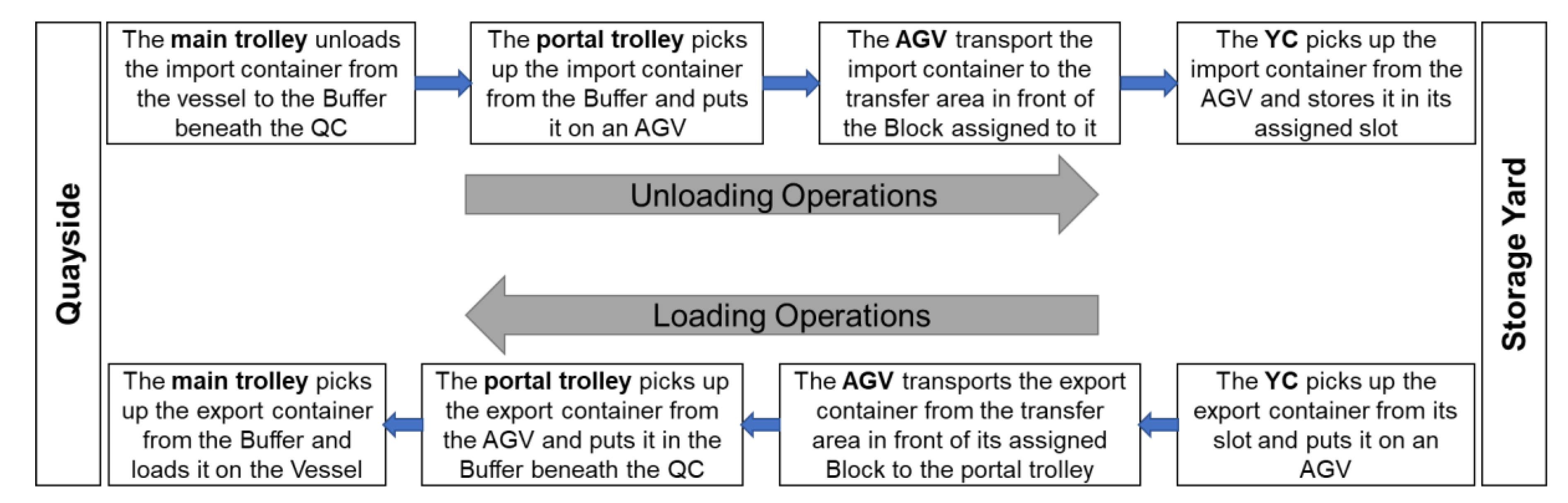
• There are four different conditions for any two consecutive containers handled by the same equipment; AGV, QC’s main trolley, or QC’s portal trolley:
  • Handling two consecutive import containers;
  • Handling two consecutive export containers;
  • Handling an export container before an import one;
  • Handling an import container before an export one.

3.2. Notations

3.2.1. Sets and Parameters

$K$	Set of QCs.
$C$	Set of YCs.
$B$	Set of yard blocks.
$N^{+}$	Set of available slots in each block.
$P$	Set of yard locations.
$N$	Set of all containers. Each container is defined by its number and its assigned quay crane.
$D$	Set of import containers (jobs), $D\subset N$
$L$	Set of export containers (jobs), $L\subset N$
$G$	Set of the containers in the buffer beneath each quay crane, $G \subset N$
$O_S$	Set of all containers beside the starting dummy container.
$O_F$	Set of all containers beside the ending dummy container.
$O$	Set of all containers, including dummy starting and ending jobs.
$k,l$	Indices for QCs.
$b,a$	Indices for blocks.
$n, n_1$	Indices for the available slots in each block.
$\left(i,k\right),\left(j,l\right)$	Indices for containers (jobs), job $\left(i,k\right)$ means that container $i$ is handled by quay crane $k$, and job $\left(j,l\right)$ means that container $j$ is handled by quay crane $l$.
$\left(S,I\right)$	Dummy starting job.
$\left(F,I\right)$	Dummy ending job.
$\left(n,b\right), \left(n_1, a\right)$	Indices for yard locations, location $\left(n,b\right)$ is slot n in block b, and location $\left(n_1,a\right)$ is slot $n_1$ in block $a$.
$h_{\left(i,k\right)}^{main}$	Handling time of container $\left(i,k\right)$ by the main trolley of its assigned quay carne.
$h_{\left(i,k\right)}^{portal}$	Handling time of container $\left(i,k\right)$ by the portal trolley of its assigned quay crane.
${\tau }_{\left(i,k\right)}$	The transportation time of AGV for export container $\left(i,k\right)$ from its assigned block to its assigned quay crane.
$t_k^b$	AGV’s transportation time from quay crane $k$ to block $b$
${\pi }_{\left(k,l\right)}$	AGV’s transportation time between quay crane $k$ and quay crane $l$.
${\rho }_{\left(i,k\right)}^b$	AGV’s traveling time from the block that container $\left(i,k\right)$ is located to block $b$, $\left(i,k\right)\in L$.
$w_{\left(i,k\right)}$	The handling time of YC to transfer export container $\left(i,k\right)$ from its assigned slot to the transfer point in front of its assigned block.
${\phi }_{\left(n,b\right)}$	The transportation time of YC between the transfer point of block b to the location $\left(n,b\right)$
${\upsilon }_{\left(n,n1\right)}$	YC’s transportation time from the assigned location of the import container $\left(i,k\right)$ to the assigned location of the import container $\left(j,l\right)$.
$M$	A large number
$B_C$	The capacity of the buffer beneath each QC
$v$	Total number of AGVs

3.2.2. Decision Variables

$x_{\left(i,k\right)}^{\left(j,l\right)}$	=1; if an AGV, scheduled to deliver the container $\left(j,l\right)$, has just delivered container $\left(i,k\right)$. =0; otherwise
$Z_{\left(i,k\right)}^{\left(n,b\right)}$	=1; if the import container $\left(i,k\right)$ is assigned to the location $\left(n,b\right)$. =0; otherwise.
${\sigma }_b{}_{\left(i,k\right)}^{\left(j,l\right)}$	=1; if the YC of block b is scheduled to handle both import containers$\left(i,k\right)$ and $\left(j,l\right)$ consecutively. =0; otherwise.
$\sigma { }_{\left(i,k\right)}^{\left(j,l\right)}$	=1; if a YC is scheduled to handle both export containers$\left(i,k\right)$ and $\left(j,l\right)$ consecutively. =0; otherwise.
${\eta }_{\left(i,j,l\right)}$	=1; if the job$i$ is located in the buffer beneath QC $l$ when the QC starts to handle job $j$ =0; otherwise.

3.2.3. Decision Variables

$u_{\left(i,k\right)}^{main}$	The starting time of the main trolley of quay crane k to handle container i
$Z_{\left(i,k\right)}^{Porter}$	The starting time of the portal trolley of quay crane k to handle container i
$d_{i,k}$	The starting time of YC to handle container (i,k)
$y_{\left(i,k\right)}^b$	=1; if block b is assigned to the import container (i,k). =0; otherwise. It is an intermediated variable: ${{\displaystyle \sum }}_{n\in N^{+}}{Z}_{\left(i,k\right)}^{\left(n,b\right)}=y_{\left(i,k\right)}^b$
$q_{i,k}$	The quay crane k’s waiting time to start handling container i
$r_{i,k}$	The AGV’s waiting time until quay crane k starts to handle container i
$A_{j,l}$	=1; if there is an available slot in the buffer beneath quay crane l when the QC starts to handle job j =0; otherwise.

3.3. Mathematical Model

Objective: Minimize the completion time of the last job.

$$\mathit{M}\mathit{i}\mathit{n}. \underset{\left(\mathit{i},\mathit{k}\right)}{\mathit{m}\mathit{a}\mathit{x}}\left({\mathit{u}}_{\left(\mathit{i},\mathit{k}\right)}^{\mathit{m}\mathit{a}\mathit{i}\mathit{n}}+{\mathit{h}}_{\left(\mathit{i},\mathit{k}\right)}^{\mathit{m}\mathit{a}\mathit{i}\mathit{n}}\right)$$

(1)

Subject to:

$${{\displaystyle \sum }}_{\left(j,l\right)\in O_F}{x}_{\left(i,k\right)}^{\left(j,l\right)}=1, \hspace{1em}\forall \left(i,k\right)\in N$$

(2)

$${{\displaystyle \sum }}_{\left(i,k\right)\in O_S}{x}_{\left(i,k\right)}^{\left(j,l\right)}=1, \hspace{1em}\forall \left(j,l\right)\in N$$

(3)

$${\displaystyle \sum }_{\left(j,l\right)\in N}{x}_{\left(S,I\right)}^{\left(j,l\right)}=v$$

(4)

$${\displaystyle \sum }_{\left(i,k\right)\in N}{x}_{\left(i,k\right)}^{\left(F,I\right)}=v$$

(5)

$$u_{\left(i+1,k\right)}^{main} \ge u_{\left(i,k\right)}^{main} + h_{\left(i,k\right)}^{main}, \hspace{1em}\forall \left(i+1,k\right), \left(i,k\right)\in N$$

(6)

$$u_{\left(i+1,k\right)}^{portal} \ge u_{\left(i,k\right)}^{portal} + h_{\left(i,k\right)}^{portal}, \hspace{1em}\forall \left(i+1,k\right), \left(i,k\right)\in N$$

(7)

$$u_{\left(i,k\right)}^{main} \ge u_{\left(i,k\right)}^{portal} + h_{\left(i,k\right)}^{portal}, \hspace{1em}\forall \left(i,k\right)\in L$$

(8)

$$u_{\left(i,k\right)}^{portal} \ge u_{\left(i,k\right)}^{main} + h_{\left(i,k\right)}^{main}, \hspace{1em}\forall \left(i,k\right)\in D$$

(9)

$$d_{\left(i,k\right)} \ge u_{\left(i,k\right)}^{portal}+h_{\left(i,k\right)}^{portal}+ {{\displaystyle \sum }}_{b\in B}{t}_k^b\ast y_{\left(i,k\right)}^b, \hspace{1em}\forall \left(i,k\right)\in D$$

(10)

$$u_{\left(i,k\right)}^{portal} \ge d_{\left(i,k\right)}+ w_{\left(i,k\right)}+ {\tau }_{\left(i,k\right)}, \hspace{1em}\forall \left(i,k\right)\in L$$

(11)

$$u_{\left(j,l\right)}^{portal}+M\ast \left(1-x_{\left(i,k\right)}^{\left(j,l\right)}\right) \ge u_{\left(i,k\right)}^{portal}, \hspace{1em}\forall \left(i,k\right), \left(j,l\right)\in N$$

(12)

$$u_{\left(j,l\right)}^{portal}+h_{\left(j,l\right)}^{portal}+M\ast \left(1-x_{\left(i,k\right)}^{\left(j,l\right)}\right)\ge d_{\left(i,k\right)}+{{\displaystyle \sum }}_{b\in B}{t}_l^b\ast y_{\left(i,k\right)}^b, \hspace{1em}\forall \left(i,k\right), \left(j,l\right)\in D$$

(13)

$$d_{\left(j,l\right)}+w_{\left(j,l\right)}+M\ast \left(1-x_{\left(i,k\right)}^{\left(j,l\right)}\right) \ge u_{\left(i,k\right)}^{portal}+{\pi }_{\left(k,l\right)}+{\tau }_{\left(j,l\right)}, \hspace{1em}\forall \left(i,k\right), \left(j,l\right)\in L$$

(14)

$$u_{\left(i,k\right)}^{portal}+{\pi }_{\left(k,l\right)} \le u_{\left(j,l\right)}^{portal}+h_{\left(j,l\right)}^{portal}+M\ast \left(1-x_{\left(i,k\right)}^{\left(j,l\right)}\right), \hspace{1em}\forall \left(i,k\right)\in L, \left(j,l\right)\in D$$

(15)

$$d_{\left(i,k\right)}+{{\displaystyle \sum }}_{b\in B}{\rho }_{\left(j,l\right)}^b\ast y_{\left(i,k\right)}^b\le d_{\left(j,l\right)}+w_{\left(j,l\right)}+M\ast \left(1-x_{\left(i,k\right)}^{\left(j,l\right)}\right),\hspace{1em}\forall \left(i,k\right)\in D, \left(j,l\right)\in L$$

(16)

$${{\displaystyle \sum }}_{\left(n,b\right)\in P}{Z}_{\left(i,k\right)}^{\left(n,b\right)}=1, \hspace{1em}\forall \left(i,k\right)\in D$$

(17)

$${{\displaystyle \sum }}_{\left(i,k\right)\in D}{Z}_{\left(i,k\right)}^{\left(n,b\right)}\le 1, \hspace{1em}\forall \left(n,b\right)\in P$$

(18)

$${{\displaystyle \sum }}_{n\in N^{+}}{Z}_{\left(i,k\right)}^{\left(n,b\right)}=y_{\left(i,k\right)}^b, \hspace{1em}\forall \left(i,k\right)\in D, \hspace{1em}\forall b\in B$$

(19)

$${{\displaystyle \sum }}_{\left(j,l\right)\in D\cup \left(F,I\right)}{{\displaystyle \sum }}_{b\in B}{\sigma }_b{}_{\left(i,k\right)}^{\left(j,l\right)}=1, \hspace{1em}\forall \left(i,k\right)\in D$$

(20)

$${{\displaystyle \sum }}_{\left(i,k\right)\in D\cup \left(S,I\right)}{{\displaystyle \sum }}_{b\in B}{\sigma }_b{}_{\left(i,k\right)}^{\left(j,l\right)}=1, \hspace{1em}\forall \left(j,l\right)\in D$$

(21)

$${{\displaystyle \sum }}_{\left(j,l\right)\in D}{\sigma }_b{}_{\left(S,I\right)}^{\left(j,l\right)}\le 1, \hspace{1em}\forall b\in B$$

(22)

$${{\displaystyle \sum }}_{\left(i,k\right)\in D}{\sigma }_b{}_{\left(i,k\right)}^{\left(F,I\right)}\le 1, \hspace{1em}\forall b\in B$$

(23)

$${\sigma }_b{}_{\left(i,k\right)}^{\left(j,l\right)}\le y_{\left(i,k\right)}^b\ast y_{\left(j,l\right)}^b, \hspace{1em}\forall \left(i,k\right), \left(j,l\right)\in D \hspace{1em}\forall b\in B$$

(24)

$$d_{\left(i,k\right)}+{{\displaystyle \sum }}_{n\in N^{+}} {\phi }_{\left(n,b\right)} \ast Z_{\left(i,k\right)}^{\left(n,b\right)}+{{\displaystyle \sum }}_{n\in N^{+} }{\upsilon }_{\left(n,n1\right)}\ast Z_{\left(i,k\right)}^{\left(n,b\right)}\ast Z_{\left(j,l\right)}^{\left(n1,b\right)} \le d_{\left(j,l\right)}+M\ast \left(1-{\sigma }_b{}_{\left(i,k\right)}^{\left(j,l\right)}\right), \hspace{1em}\forall \left(i,k\right), \left(j,l\right)\in D \forall b\in B$$

(25)

$${{\displaystyle \sum }}_{\left(j,l\right)\in L\cup \left(F,I\right)}{\sigma }_{\left(i,k\right)}^{\left(j,l\right)}=1, \hspace{1em}\forall \left(i,k\right)\in L$$

(26)

$${{\displaystyle \sum }}_{\left(i,k\right)\in L\cup \left(S,I\right)}{\sigma }_{\left(i,k\right)}^{\left(j,l\right)}=1, \hspace{1em}\forall \left(j,l\right)\in L$$

(27)

$${{\displaystyle \sum }}_{\left(j,l\right)\in L}{\sigma }_{\left(S,I\right)}^{\left(j,l\right)}=c,$$

(28)

$${{\displaystyle \sum }}_{\left(i,k\right)\in L}{\sigma }_{\left(i,k\right)}^{\left(F,I\right)}=c,$$

(29)

$$d_{\left(i,k\right)}+w_{\left(i,k\right)}+{\beta }_{\left(i,k\right)}^{\left(j,l\right)}\le d_{\left(j,l\right)}+M\ast \left(1-{\sigma }_{\left(i,k\right)}^{\left(j,l\right)}\right), \hspace{1em}\forall \left(i,k\right), \left(j,l\right)\in L$$

(30)

$$q_{\left(i+1,k\right)}\ge u_{\left(i+1,k\right)}^{main} -u_{\left(i,k\right)}^{main} -h_{\left(i,k\right)}^{main}, \hspace{1em}\forall \left(i,k\right)\in N$$

(31)

$$r_{\left(i,k\right)}=u_{\left(i,k\right)}^{portal}-d_{\left(i,k\right)}-w_{\left(i,k\right)}-{\tau }_{\left(i,k\right)}, \hspace{1em}\forall \left(i,k\right)\in L$$

(32)

$$r_{\left(j,l\right)}+M\ast \left(1-x_{\left(i,k\right)}^{\left(j,l\right)}\right)\ge u_{\left(j,l\right)}^{portal}+h_{\left(j,l\right)}^{portal}-d_{\left(i,k\right)}-{{\displaystyle \sum }}_{b\in B} t_l^b\ast y_{\left(i,k\right)}^b, \hspace{1em}\forall \left(i,k\right), \left(j,l\right)\in D$$

(33)

$$r_{\left(j,l\right)}+M\ast \left(1-x_{\left(i,k\right)}^{\left(j,l\right)}\right)\ge u_{\left(j,l\right)}^{portal}+h_{\left(j,l\right)}^{portal}-u_{\left(i,k\right)}^{portal}-{\pi }_{\left(k,l\right)}, \hspace{1em}\forall \left(i,k\right)\in L, \left(j,l\right)\in D$$

(34)

$$M\ast {\eta }_{\left(i,j,l\right)}\ge u_{\left(i,k\right)}^{main}-u_{\left(j,l\right)}^{portal}-h_{\left(j,l\right)}^{portal}, \hspace{1em}\forall \left(i,k\right), \left(j,l\right)\in L, k=l, j>i$$

(35)

$$M\ast {\eta }_{\left(i,j,l\right)}\ge u_{\left(i,k\right)}^{portal}-u_{\left(j,l\right)}^{portal}-h_{\left(j,l\right)}^{portal}, \hspace{1em}\forall \left(i,k\right)\in D, \left(j,l\right)\in L, k=l, j>i$$

(36)

$$M\ast {\eta }_{\left(i,j,l\right)}\ge u_{\left(i,k\right)}^{main}-u_{\left(j,l\right)}^{main}-h_{\left(j,l\right)}^{main}, \hspace{1em}\forall \left(i,k\right)\in L, \left(j,l\right)\in D, k=l, j>i$$

(37)

$$M\ast {\eta }_{\left(i,j,l\right)}\ge u_{\left(i,k\right)}^{portal}-u_{\left(j,l\right)}^{main}-h_{\left(j,l\right)}^{main}, \hspace{1em}\forall \left(i,k\right)\in D, \left(j,l\right)\in D, k=l, j>i$$

(38)

$$M\ast A_{\left(j,l\right)}\ge B_C-{{\displaystyle \sum }}_{i<j}{\eta }_{\left(i,j,l\right)} , \hspace{1em}\forall \left(j,l\right)\in N$$

(39)

$$M\ast \left(1-A_{\left(j,l\right)}\right)\ge {{\displaystyle \sum }}_{i<j}{\eta }_{\left(i,j,l\right)}-B_C , \hspace{1em}\forall \left(j,l\right)\in N$$

(40)

$$u_{\left(j,l\right)}^{portal}+M\ast A_{\left(j,l\right)}\ge u_{\left(i,k\right)}^{main}, \hspace{1em}\forall \left(j,l\right), \left(i,k\right)\in L, k=l, i=j-B_C$$

(41)

$$u_{\left(j,l\right)}^{portal}+M\ast A_{\left(j,l\right)}\ge u_{\left(i,k\right)}^{portal}, \hspace{1em}\forall \left(j,l\right)\in L, \left(i,k\right)\in D, k=l, i=j-B_C$$

(42)

$$u_{\left(j,l\right)}^{main}+M\ast A_{\left(j,l\right)}\ge u_{\left(i,k\right)}^{main}, \hspace{1em}\forall \left(j,l\right)\in D, \left(i,k\right)\in L, k=l, i=j-B_C$$

(43)

$$u_{\left(j,l\right)}^{main}+M\ast A_{\left(j,l\right)}\ge u_{\left(i,k\right)}^{portal}, \hspace{1em}\forall \left(j,l\right), \left(i,l\right)\in D, k=l, i=j-B_C$$

(44)

$$u_{\left(i,k\right)}^{portal}, u_{\left(i,k\right)}^{main}, d_{\left(i,k\right)}, q_{\left(i,k\right)}, r_{\left(i,k\right)}, v \ge 0, \hspace{1em}\forall \left(i,k\right)\in N$$

(45)

$$x_{\left(i,k\right)}^{\left(j,l\right)}, y_{\left(i,k\right)}^b, Z_{\left(i,k\right)}^{\left(n,b\right)}, {\sigma }_b{}_{\left(i,k\right)}^{\left(j,l\right)}, S_{\left(i,j,l\right)}, A_{\left(j,l\right)}\in \left\{0,1\right\}, \hspace{1em}\forall \left(i,k\right),\left(j,l\right)\in O, \forall \left(n,b\right)\in P, \forall b\in B$$

(46)

This model aims to minimize the completion time of all containers. Constraints (2) and (3) ensure that an AGV can handle, at most, one container at a time. Constraints (4) and (5) ensure that the number of AGVs is exactly (𝑣). In other words, they guarantee that the used number of AGVs cannot exceed the number of available AGVs. Constraints (6) and (7) ensure that the main trolley and the portal trolley of QC (𝑘) cannot start handling the container $\left(i+1\right)$ until finishing the current one (𝑖), respectively.

Constraints (8) to (16) regulate the interference among QCs, AGVs, and YCs. Constraint (8) illustrates that for each export container (𝑖,𝑘)∈𝐿, the main trolley of the QC (𝑘) can start handling the container after it arrives at the buffer beneath the QC by the portal trolley. Constraint (9) states that for each import container (𝑖,𝑘)∈D, the portal trolley of the QC (𝑘) can start handling the container after it arrives at the buffer beneath the QC by the main trolley. Constraint (10) implies that for each import container (𝑖,𝑘)∈𝐷, the YC can start handling the container just after it arrives at the transfer point in front of the block (𝑏).

Constraint (11) implies that for each export container (𝑖,𝑘)∈𝐿, the portal trolley of QC (𝑘) can start picking it up from the AGV after it arrives at the quayside. Constraint (12) guarantees that the AGVs’ scheduling conforms to the QCs’ scheduling. Constraints (13) to (16) are used to regulate the starting time of any two successive containers transported by the same AGV under the various transportation situations: transporting two successive import containers, transporting two successive export containers, transporting an export container just before an import, and transporting an import container just before an export container. However, the value of M is calculated as a number larger than the completion time of the last job.

Constraints (17) to (24) allocate the import containers in the yard and schedule the YCs’ handling operations. Constraints (17) and (18) ensure that each import container is assigned to only one slot in the yard, while constraint (19) is an intermediate constraint that represents the relation between the two decision variables $y_{\left(i,k\right)}^b$and $Z_{\left(i,k\right)}^{\left(n,b\right)}$.

Constraints (20) and (21) state that each import container is handled just before a container (𝑗,𝑙)∈𝐷∪(𝐹,𝐼), and just after a container (𝑖,𝑘)∈𝐷∪(𝑆,𝐼) by the same YC. In other words, they ensure that a YC can handle at most one container at a time. Constraints (22) and (23) indicate that each block’s scheduling process should start and end with dummy jobs/containers to prevent symmetric solutions. Constraint (24) ensures that ${\sigma }_b{}_{\left(i,k\right)}^{\left(j,l\right)}=1$ if containers (𝑖,𝑘) and (𝑗,𝑙) are assigned to the same block.

Constraint (25) regulates the time between two consecutive import containers handled by the same YC. On the other hand, constraints from (26) to (29) are used to schedule export containers on the YCs. Constraint (30) regulates the time between two successive export containers handled by the same yard crane.

Moreover, constraint (31) calculates the QC’s waiting time to handle the container (𝑖,𝑘), which is the difference between the actual starting and the earliest starting time. Constraints (32) to (34) calculate the waiting time of AGVs at the quayside. Constraints from (35) to (38) determine if the container $i$ is in the buffer when the container $j$ is handled under the various handling conditions: handling two successive import containers, handling two successive export containers, handling an export container just before an import, and handling an import container just before an export container. Constraints (39) and (40) determine if the container $\left(j\right)$ can be handled by the QC or has to wait until there is available space in the buffer beneath the QC. Constraints (41) and (42) ensure that the portal trolley of QC $\left(l\right)$cannot handle the export container$\left(j\right)$until there is available space in the buffer beneath the QC. Constraints (43) and (44) ensure that the main trolley of QC $\left(l\right)$ cannot handle the import container$\left(j\right)$until there is available space in the buffer beneath the QC. Finally, Constraints (45) and (46) are non-negativity and binary constraints. However, starting and ending dummy jobs is crucial to prevent the symmetric solutions in scheduling YCs and AGVs.

4. Results and Discussion

A set of 14 instances were used to test the performance of the proposed MIP model. The parameters of the instances were based on [6,27] and modified to suit the developed model. The handling times, φ(n,b) and w(i,k), of each YC from each container’s location to the transfer point in front of the block, follow a uniform distribution 𝑈(60,140)s. The processing times, $h_{\left(i,k\right)}^{main}$, of each main trolley of QC follows a uniform distribution 𝑈(30,150)s and the processing time, $h_{\left(i,k\right)}^{portal}$, of each portal trolley of QC was constant for all QCs and equal to 30 s. The buffer capacity beneath each QC was five, and the number of QCs used in each instance was two. For any given instance, the number of variables (V) and the number of constraints (R) could be calculated using the following two formulas:

$$V=N\left(N+1\right)+L^2+D\left(D+P\right)$$

(47)

$$R=N\left(5+2\left(N-1\right)\right)+{\left(N-1\right)}^2+L\left(3+7D\right)+{\left(L-1\right)}^2+{\left(D-1\right)}^2\ast \left(2B+3\right)+6D+3B+P+4$$

(48)

where N, P, L, D, and B are the maximum indices of all containers, yard locations, export containers, import containers, and blocks, respectively. Gurobi 9.1.0 optimization software(Gurobi optimization, Beaverton, OR, USA) was used to solve all instances on a computer with an Intel Core™ i7 processor (Intel Corporation, Santa Clara, CA, USA). Ten runs were performed using the same parameter settings for each instance, and the average value of these ten runs is reported. The computational time for all instances was limited to 3000 s, common in most research studies [8].

The key bottleneck resource in this problem was the limited buffer capacity beneath the QCs. Therefore, the instances were designed for three main purposes:

• Investigating the effect of the integrating the scheduling of YCs and AGVs considering the limited QCs buffer capacity on completion time, AGV utilization, and QC utilization;
• Investigating the effects of using the QCs buffer capacity with different sizes;
• Investigating the impact of using single-trolley QCs instead of dual-trolley QCs.

4.1. Investigating the Effect of the Integrating the Scheduling of YCs and AGVs on Completion Time, AGV Utilization, and QC Utilization

Table 1. Computational results for dual-trolley QCs with a buffer capacity equal to five.

Instances	Number of Containers	AGV/YC	Optimum Solution
			Computational Time (s)	Completion Time (s)	Average AGV Waiting Time (s)	Average QC Waiting Time (s)	AGV Utilization (%)	QC Utilization (%)
1	5	2/2	0.016	519	64.95	382	87.49	26.40
2	6	2/2	0.021	602	60	376	90.03	37.54
3	10	2/2	0.202	994	78	588	92.15	40.85
4	10	3/2	0.073	794	127	413	84.01	47.98
5	15	3/2	0.596	998	120	485	87.98	51.40
6	20	3/2	8	1451	159	626	89.04	56.86
7	25	3/2	46	1808	190	787	89.49	56.47
8	25	3/3	59	1793	183	756	89.79	57.84
9	25	5/3	5	1479	310	455	79.04	69.24
10	30	5/3	11	1809	263	570	85.46	68.49
11	40	6/4	110	2002	309	235	84.57	88.26
12	50	6/4	711	2261	358	262	84.84	88.90
13	60	6/4	1324	2822	409	325	85.51	88.48
14	70	6/4	---	---	---	---	---	---

shows the results of solving the instances using the proposed MIP model with a QC buffer capacity equal to five. The number of containers in each instance and the number of AGVs and YCs are reported. The optimum solution is represented by the completion time of the last job measured in (s), the average QC waiting time measured in (s), and the average AGV waiting time measured in (s). The results of different instances cannot be compared using the waiting time of the equipment only as it is a portion of the completion time. Thus, QC utilization and AGV utilization for each instance were calculated for a proper comparison. The AGV and QC utilizations were calculated using Formulas (49) and (50), respectively.

$$AGV utilization=\frac{Completion time-AGV waiting time}{Completion time} \ast 100$$

(49)

$$QC utilization =\frac{Completion time-QC waiting time}{Completion time} \ast 100$$

(50)

From Table 1, although all the results increased with the increasing number of containers, there was a significant impact on the results when changing the number of resources to serve the same number of containers; as in instance 4 compared with instance 3, and instances 8 and 9 compared with instance 7. In instance 4, AGVs increased from two to three to serve the same number of containers. In instance 8, the number of YCs increased to three instead of two, while in instance 9, the number of AGVs increased to five instead of three. The computational time decreased in instances 4 and 9 because of the increasing number of AGVs. That is because the number of resources increased, so the model relaxed.

The completion time dropped with the increasing number of resources, as a larger number of resources served the same number of containers. Additionally, QC utilization increased with the increasing number of resources because QCs had to wait for a shorter time for AGVs to become available. On the contrary, AGV utilization decreased with the increasing number of AGVs as a larger number of AGVs served the same number of containers, leading to an increase in AGV waiting time. Although increasing AGV number significantly impacted completion time and QC waiting time, it negatively affected the terminal. That is because it increased traffic leading to congestion, collision, and bottlenecks. Therefore, the number of vehicles should be limited to be within the carrying capacity of the terminal. Therefore, terminals use dual-trolley QCs to help in solving this issue. According to instance 14, the computational time was unreasonably high due to the complexity of the instance with a high number of containers because the problem was an NP-hard problem. In other words, 70 containers were too large to be solved optimally by the MIP model in a reasonable time.

One of the runs of instance 4 is used as an example to illustrate the scheduling of the equipment used and the assignment of storage locations for import containers, as shown in Figure 4. The storage locations of the import containers are defined by the block number, which equals the YC number and the slot number.

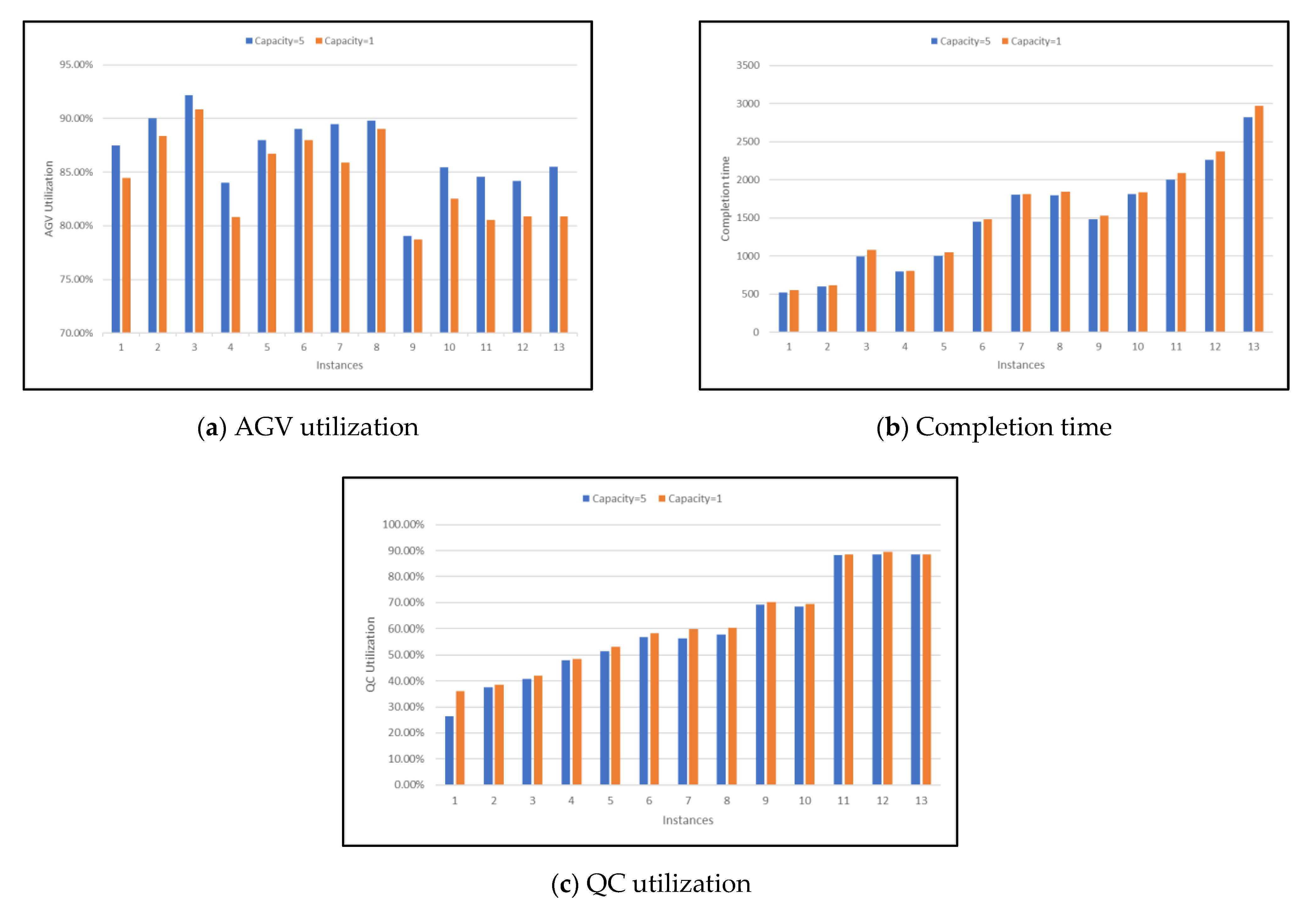
4.2. Investigating the Effect of Using the QC Buffer Capacity with Different Sizes

Table 2. Computational results for dual-trolley QCs with a buffer capacity equal to one.

Instances	Number of Containers	AGV/YC	Optimum Solution
			Computational Time (s)	Completion Time (s)	AGV Utilization (%)	QC Utilization (%)
1	5	2/2	0.009	553	84.45	35.99
2	6	2/2	0.02	620	88.39	33.71
3	10	2/2	0.191	1079	90.82	41.89
4	10	3/2	0.05	808	80.82	48.39
5	15	3/2	0.563	1052	86.69	53.23
6	20	3/2	6.513	1483	88.00	58.26
7	25	3/2	30.999	1810	85.91	59.89
8	25	3/3	21.667	1842	89.03	60.26
9	25	5/3	2.5	1532	78.72	70.23
10	30	5/3	11.04	1833	82.54	69.50
11	40	6/4	94.535	2091	80.54	88.47
12	50	6/4	272.419	2374	80.88	89.51
13	60	6/4	1431.354	2971	80.88	88.59

illustrates the results of solving the instances using the proposed MIP model with a QCs buffer capacity equal to one. The comparison between using a QCs buffer capacity equal to five or one is shown in Figure 5a–c. The QCs buffer size significantly impacted AGV utilization, as shown in Figure 5a. The figure shows that the AGV utilization for the higher QCs buffer capacity was much more than the lower one. On the contrary, the QCs buffer capacity size slightly affected both completion time and QC utilization, as shown in Figure 5b,c, respectively. According to the completion time, the higher QCs buffer capacity always gave a better completion time, and it appeared clearly with the increasing size of the problem, as in instance 13. At the same time, QC utilization was almost the same for the two capacities. The reason is that the main trolley QC operates on is much slower than the portal trolley, so there was always a container in the buffer to handle. Additionally, the QC scheduling was assumed to be known in advance, so the completion time was insignificantly changed.

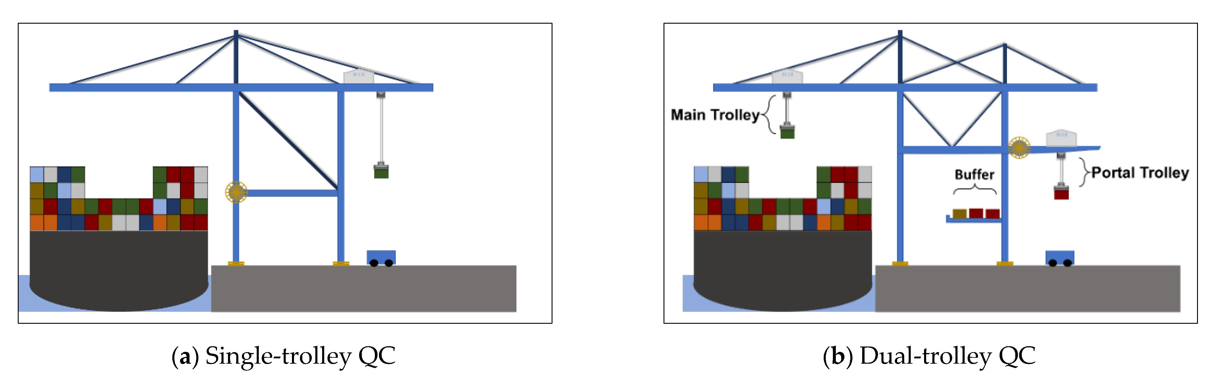
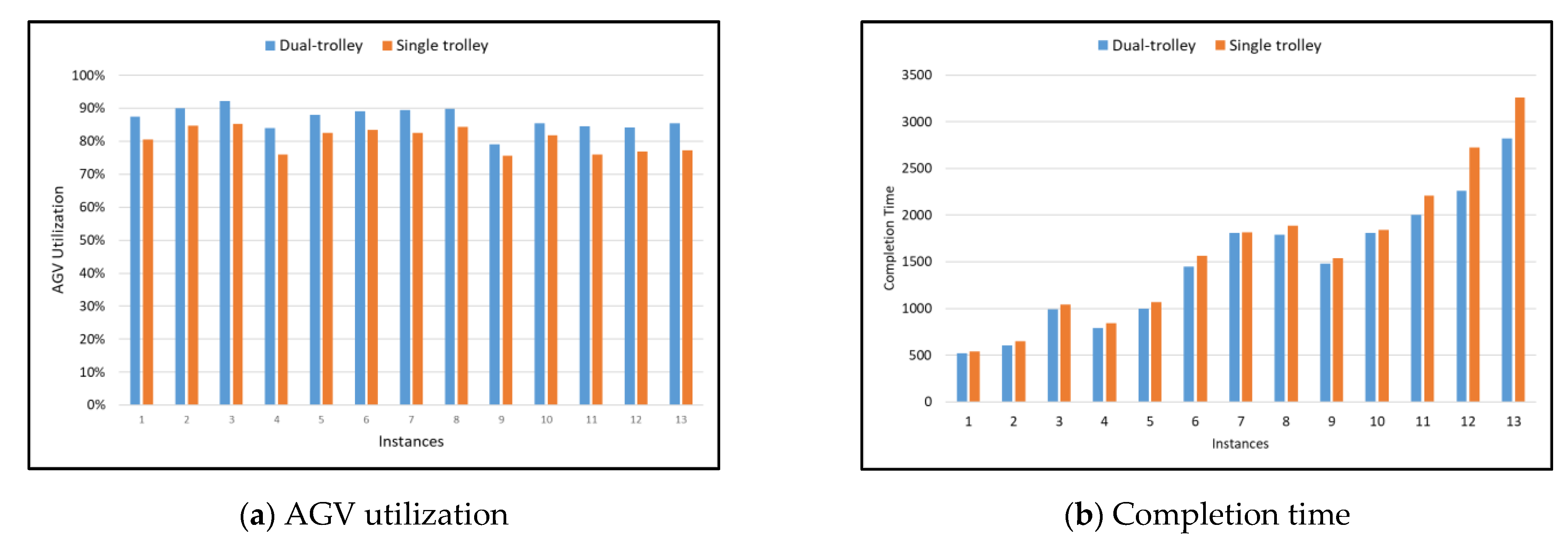
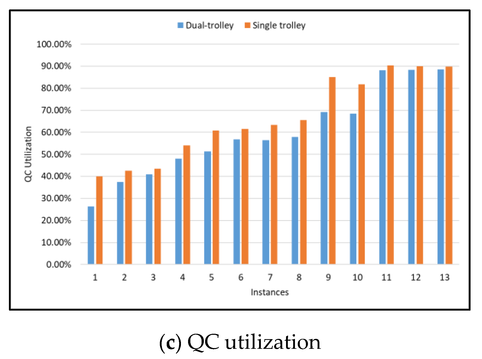
4.3. Investigating the Impact of Using Single-Trolley QCs Instead of Dual-Trolley QCs

Table 3. Computational results for single-trolley QCs.

Instances	Number of Containers	AGV/YC	Optimum Solution
			Computational Time (s)	Completion Time (s)	AGV Utilization (%)	QC Utilization (%)
1	5	2/2	0.009	543.00	80.48	39.96
2	6	2/2	0.025	651	84.79	42.55
3	10	2/2	2	1045	85.36	43.44
4	10	3/2	0.074	845	75.98	54.08
5	15	3/2	0.646	1066	82.55	60.88
6	20	3/2	13	1565	83.39	61.47
7	25	3/2	70	1817	82.61	63.29
8	25	3/3	66	1889	84.33	65.64
9	25	5/3	3	1541	75.60	85.01
10	30	5/3	13	1843	81.88	81.71
11	40	6/4	82	2210	76.02	90.41
12	50	6/4	236	2728	76.83	89.96
13	60	6/4	449	3259	77.29	89.90

shows the results of solving the instances using the proposed MIP model with single-trolley QCs. The comparison between using single-trolley QCs and dual-trolley QCs with a buffer capacity equal to five is shown in Figure 6. The results show that dual-trolley QC significantly increased the AGV utilization and decreased the completion time of the last job, as shown in Figure 6a,b, respectively. While it decreased the QC utilization, as shown in Figure 6c. The reason for this is the portal trolley had to wait until an available slot to put the container in the buffer, as in the case of export containers, or the main trolley had to wait for an available slot in the case of import containers.

In summary, these experiments indicate that the dual-trolley QCs significantly affect the vessel berthing time and the congestion at the quayside by reducing the completion time of the last container and the waiting time of AGVs. Additionally, the QCs buffer capacity is a critical bottleneck resource. Therefore, automated container terminal managers should install dual-trolley QCs instead of the single-trolley and increase their buffer capacities.

5. Conclusions and Future Work

The performance of a container terminal is mainly measured by the vessel berthing time and is highly affected by the scheduling of different equipment. One of the most challenging problems both scholars and terminal operators face is introducing a proper scheduling plan for different equipment, considering the buffer capacity of dual-trolley QCs and the limited storage locations of import containers. Therefore, this article proposed a mixed integer programming model to integrate the scheduling of YCs and AGVs, considering the allocation of import containers. Additionally, the model introduced a novel set of constraints to consider the buffer capacity beneath QCs. The QCs buffer capacity constraints were determined when handling each container to make the model more general and applicable under any condition. For example, a check must be performed to ensure a slot is available in the buffer if a particular container has to be handled. Otherwise, the container has to wait for a slot to be available. The objective was to minimize the completion time of the last job, which significantly affects the vessel berthing time. Several numerical experiments were implemented to analyze the studied problem and test the performance of the proposed model.

The results provide detailed scheduling and assigning plans for YCs and AGVs besides allocating import containers in a specific slot and block. The results show that the completion time dropped with the increasing number of resources (i.e., YCs and AGVs) as more resources serve the same number of containers. Additionally, QC utilization increased with the increasing number of resources because QCs had to wait for a shorter time for AGVs to become available. On the contrary, AGV utilization decreased with an increase in its number as the waiting time of AGVs increased. Although increasing the number of AGVs significantly impacted the completion time of the last job and QC utilization, it negatively affected the terminal because it increased traffic leading to congestion, collision, and bottlenecks. So, the number of vehicles should be limited to be within the carrying capacity of the terminal. Hence, terminals should use dual-trolley QCs to help in solving this issue. However, it is clear from the results that dual-trolley QCs decrease the completion time and increase AGV utilization compared to single-trolley QCs. Additionally, the completion time decreased with the increasing capacity size of the buffer beneath dual-trolley QCs, while AGV utilization increased.

For future work, the scheduling of both trolleys of QCs can be included in the model. The effect of using different QC buffer capacity sizes can be studied. Heuristics can be implemented to solve large instances. Obtaining the optimum capacity size of the buffer beneath each QC can be included in the model. Pareto analysis can be conducted to introduce suitable tradeoffs for increasing QC utilization and decreasing the completion time of all jobs. Moreover, minimizing the QC waiting time can be considered in the model as an objective function.

References

1. Han, E.S.; Goleman, D.; Boyatzis, R.; Mckee, A. Review of Maritime Transport 2020; United Nations: New York, NY, USA, 2020; Volume 53. [Google Scholar]
2. Naeem, D.; Gheith, M.; Eltawil, A. Integrated Scheduling of AGVs and Yard Cranes in Automated Container Terminals. In Proceedings of the 2021 IEEE 8th International Conference on Industrial Engineering and Applications (ICIEA), Chengdu, China, 23–26 April 2021; pp. 632–636. [Google Scholar] [CrossRef]
3. Lu, Y. The Three-Stage Integrated Optimization of Automated Container Terminal Scheduling Based on Improved Genetic Algorithm. Math. Probl. Eng. 2021, 2021, 6792137. [Google Scholar] [CrossRef]
4. Hu, H.; Chen, X.; Wang, T.; Zhang, Y. A Three-Stage Decomposition Method for the Joint Vehicle Dispatching and Storage Allocation Problem in Automated Container Terminals. Comput. Ind. Eng. 2019, 129, 90–101. [Google Scholar] [CrossRef]
5. Yu, H.; Deng, Y.; Zhang, L.; Xiao, X.; Tan, C. Yard Operations and Management in Automated Container Terminals: A Review. Sustainability 2022, 14, 3419. [Google Scholar] [CrossRef]
6. Luo, J.; Wu, Y. Scheduling of Container-Handling Equipment during the Loading Process at an Automated Container Terminal. Comput. Ind. Eng. 2020, 149, 106848. [Google Scholar] [CrossRef]
7. Luo, J.; Wu, Y.; Mendes, A.B. Modelling of Integrated Vehicle Scheduling and Container Storage Problems in Unloading Process at an Automated Container Terminal. Comput. Ind. Eng. 2016, 94, 32–44. [Google Scholar] [CrossRef]
8. Luo, J.; Wu, Y. Modelling of Dual-Cycle Strategy for Container Storage and Vehicle Scheduling Problems at Automated Container Terminals. Transp. Res. Part E Logist. Transp. Rev. 2015, 79, 49–64. [Google Scholar] [CrossRef]
9. Gheith, M.; Eltawil, A.B.; Harraz, N.A. Solving the Container Pre-Marshalling Problem Using Variable Length Genetic Algorithms. Eng. Optim. 2016, 48, 687–705. [Google Scholar] [CrossRef]
10. Iris, Ç.; Pacino, D.; Ropke, S.; Larsen, A. Integrated Berth Allocation and Quay Crane Assignment Problem: Set Partitioning Models and Computational Results. Transp. Res. Part E Logist. Transp. Rev. 2015, 81, 75–97. [Google Scholar] [CrossRef] [Green Version]
11. Li, C.-L. Managing Navigation Channel Traffic and Anchorage Area Utilization of a Container Port. Transp. Sci. 2019, 53, 728–745. [Google Scholar] [CrossRef]
12. Jia, S.; Li, C.L.; Xu, Z. A Simulation Optimization Method for Deep-Sea Vessel Berth Planning and Feeder Arrival Scheduling at a Container Port. Transp. Res. Part B Methodol. 2020, 142, 174–196. [Google Scholar] [CrossRef]
13. Li, S.; Jia, S. The Seaport Traffic Scheduling Problem: Formulations and a Column-Row Generation Algorithm. Transp. Res. Part B Methodol. 2019, 128, 158–184. [Google Scholar] [CrossRef]
14. ElWakil, M.; Gheith, M.; Eltawil, A. A New Hybrid Salp Swarm-Simulated Annealing Algorithm for the Container Stacking Problem. In Proceedings of the 9th International Conference on Operations Research and Enterprise Systems, Valletta, Malta, 22–24 February 2020; pp. 89–99. [Google Scholar] [CrossRef]
15. Yue, L.; Fan, H.; Ma, M. Optimizing Configuration and Scheduling of Double 40 Ft Dual-Trolley Quay Cranes and AGVs for Improving Container Terminal Services. J. Clean. Prod. 2021, 292, 126019. [Google Scholar] [CrossRef]
16. Karam, A.; Eltawil, A.B. Functional Integration Approach for the Berth Allocation, Quay Crane Assignment and Specific Quay Crane Assignment Problems. Comput. Ind. Eng. 2016, 102, 458–466. [Google Scholar] [CrossRef]
17. Karam, A.; Eltawil, A.B. A Lagrangian Relaxation Approach for the Integrated Quay Crane and Internal Truck Assignment in Container Terminals. Int. J. Logist. Syst. Manag. 2016, 24, 113–136. [Google Scholar] [CrossRef]
18. Sadeghian, S.H.; bin Mohd Ariffin, M.K.A.; Hong, T.S.; bt Ismail, N. Integrated Scheduling of Quay Cranes and Automated Lifting Vehicles in Automated Container Terminal with Unlimited Buffer Space. In Advances in Systems Science; Swiatek, J., Grzech, A., Swiątek, P., Tomczak, J.M., Eds.; Springer International Publishing: New York, NY, USA, 2014. [Google Scholar]
19. Kress, D.; Meiswinkel, S.; Pesch, E. Straddle Carrier Routing at Seaport Container Terminals in the Presence of Short Term Quay Crane Buffer Areas. Eur. J. Oper. Res. 2019, 279, 732–750. [Google Scholar] [CrossRef]
20. Castilla-Rodríguez, I.; Expósito-Izquierdo, C.; Melián-Batista, B.; Aguilar, R.M.; Moreno-Vega, J.M. Simulation-Optimization for the Management of the Transshipment Operations at Maritime Container Terminals. Expert. Syst. Appl. 2020, 139. [Google Scholar] [CrossRef]
21. Duinkerken, M.B.; Evers, J.J.M.; Ottjes, J.A. A Simulation Model for Integrating Quay Transport and Stacking Policies on Automated Container Terminals. In Proceedings of the 15th European Simulation Multiconference, San Diego, CA, USA, 1 June 2001; pp. 909–916. [Google Scholar]
22. Lau, H.Y.K.; Zhao, Y. Integrated Scheduling of Handling Equipment at Automated Container Terminals. Int. J. Prod. Econ. 2008, 112, 665–682. [Google Scholar] [CrossRef]
23. Yang, Y.; Zhong, M.; Dessouky, Y.; Postolache, O. An Integrated Scheduling Method for AGV Routing in Automated Container Terminals. Comput. Ind. Eng. 2018, 126, 482–493. [Google Scholar] [CrossRef]
24. Zhao, Q.; Ji, S.; Guo, D.; Du, X.; Wang, H. Research on Cooperative Scheduling of Automated Quayside Cranes and Automatic Guided Vehicles in Automated Container Terminal. Math. Probl. Eng. 2019, 2019, 6574582. [Google Scholar] [CrossRef]
25. Yue, L.; Fan, H.; Zhai, C. Joint Configuration and Scheduling Optimization of the Dual Trolley Quay Crane and AGV for Automated Container Terminal. In Proceedings of the 2019 4th International Seminar on Computer Technology, Mechanical and Electrical Engineering (ISCME 2019), Chengdu, China, 13–15 December 2019; Volume 1486. [Google Scholar] [CrossRef]
26. Li, H.; Peng, J.; Wang, X.; Wan, J. Integrated Resource Assignment and Scheduling Optimization with Limited Critical Equipment Constraints at an Automated Container Terminal. IEEE Trans. Intell. Transp. Syst. 2021, 22, 7607–7618. [Google Scholar] [CrossRef]
27. Xu, B.; Jie, D.; Li, J.; Yang, Y.; Wen, F.; Song, H. Integrated Scheduling Optimization of U-Shaped Automated Container Terminal under Loading and Unloading Mode. Comput. Ind. Eng. 2021, 162, 107695. [Google Scholar] [CrossRef]
28. Lu, Y. The Optimization of Automated Container Terminal Scheduling Based on Proportional Fair Priority. Math. Probl. Eng. 2022, 2022, 7889048. [Google Scholar] [CrossRef]
29. Qin, T.; Du, Y.; Chen, J.H.; Sha, M. Combining Mixed Integer Programming and Constraint Programming to Solve the Integrated Scheduling Problem of Container Handling Operations of a Single Vessel. Eur. J. Oper. Res. 2020, 285, 884–901. [Google Scholar] [CrossRef]
Figure 1. Types of QCs in ACTs (a,b).
Logistics 06 00082 g001
Figure 2. A typical layout of an ACT.
Logistics 06 00082 g002
Figure 3. Loading and unloading operations in an ACT.
Logistics 06 00082 g003
Figure 4. Gantt chart for all equipment used.
Logistics 06 00082 g004
Figure 5. Comparison of using the QCs buffer capacity equal to five or one (ac).
Logistics 06 00082 g005
Figure 6. Comparison of using dual-trolley QCs and single-trolley QC (ac).
Logistics 06 00082 g006aLogistics 06 00082 g006b