
Fortran Coarray Implementation of Semi-Lagrangian Convected Air Particles within an Atmospheric Model


Abstract
:1. Introduction
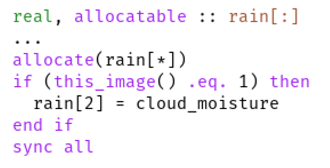
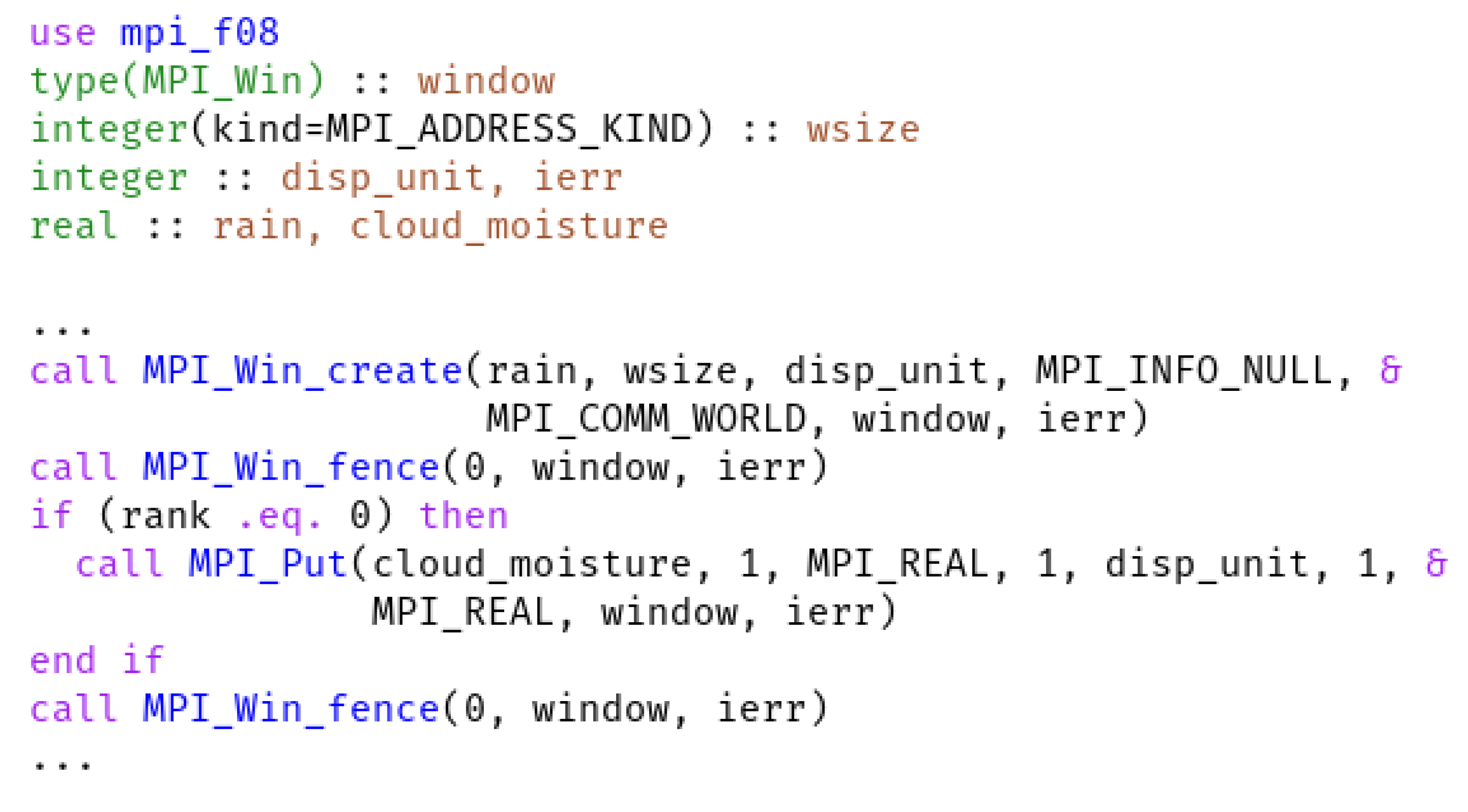
1.1. Fortran Coarrays
1.2. Convection
2. Materials and Methods
2.1. Air Particle Physics
2.1.1. Lapse Rate
2.1.2. Orographic Lifting
2.2. Methodology
2.3. Hardware and Software
- call assign(‘‘assign -S on -y on p:\%.txt’’, ierrr)
Profiling Tools
3. Results and Discussions
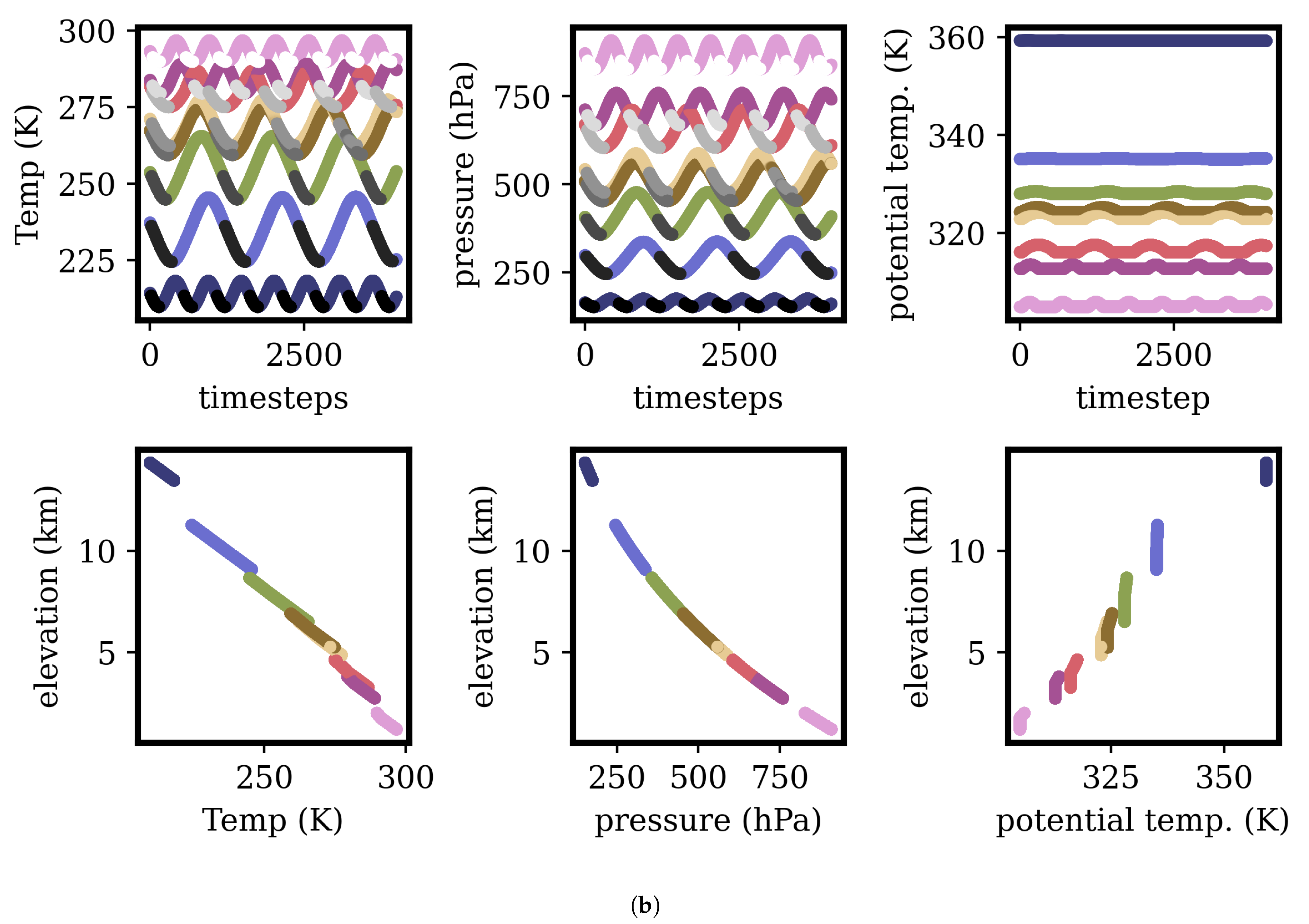
3.1. Validation
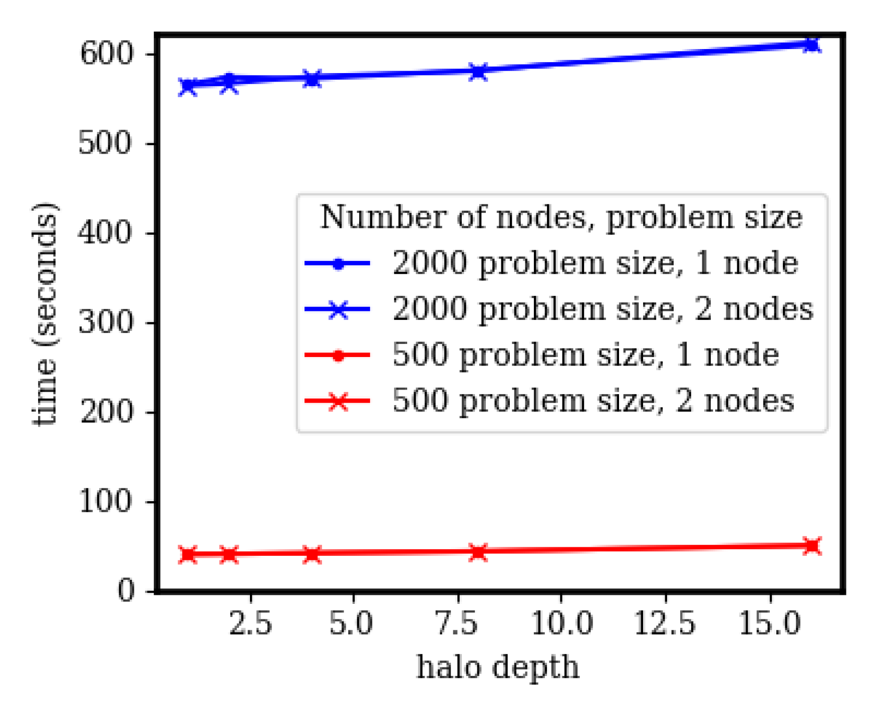
3.2. Halo Depth
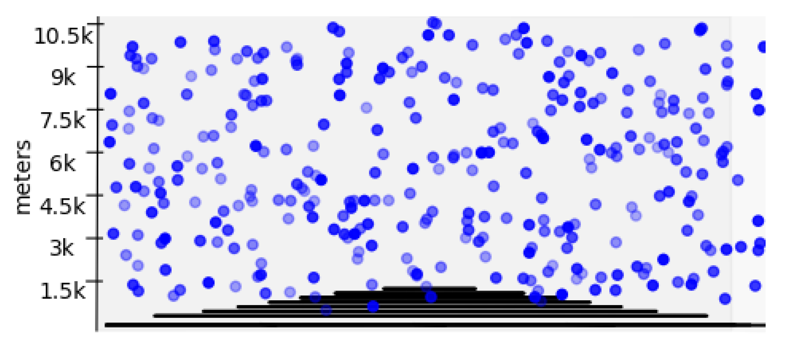
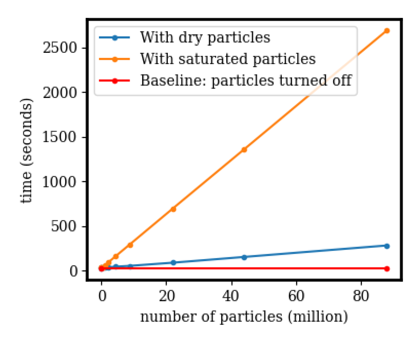
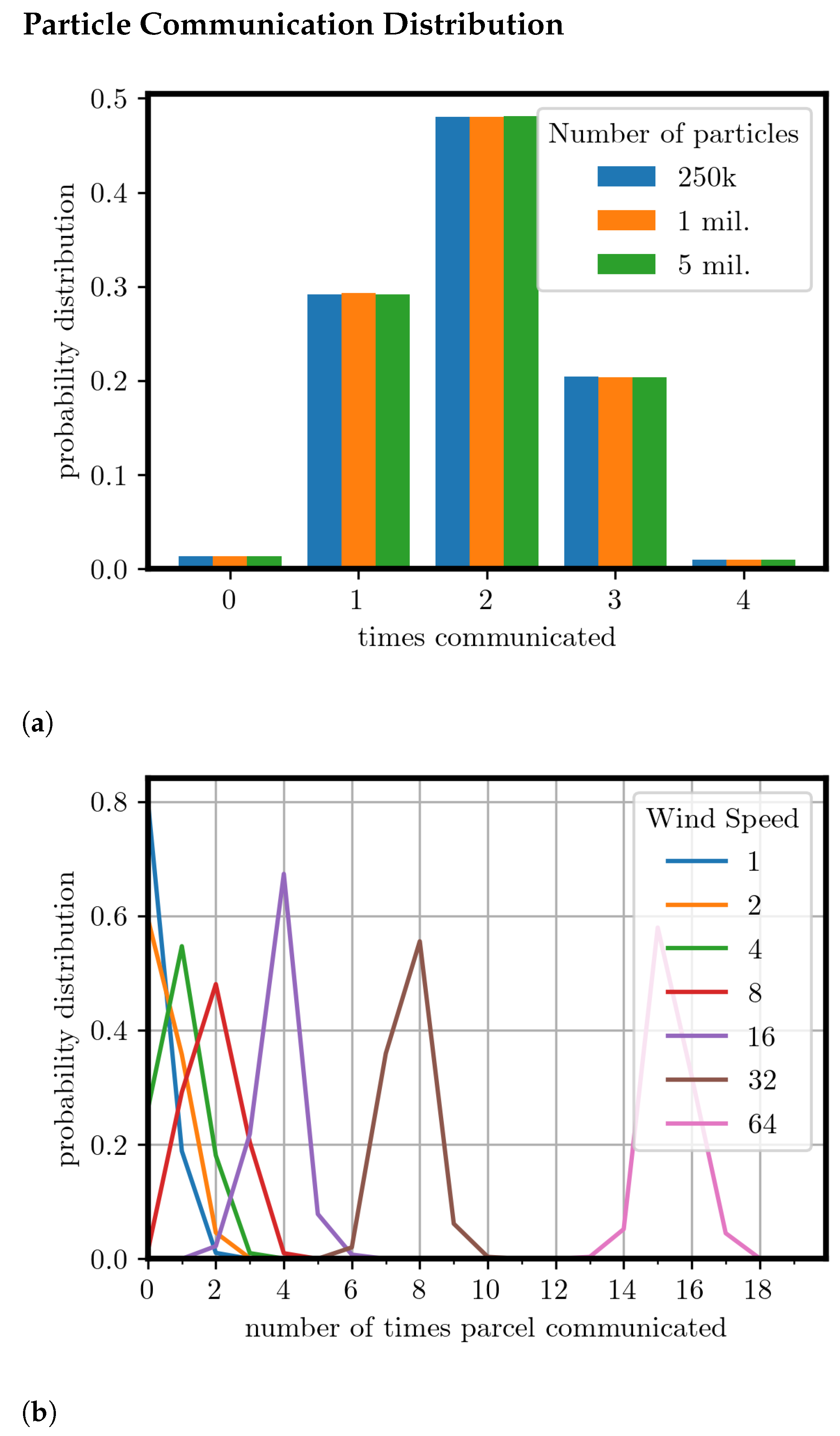
3.3. Particle Count and Wind Speed
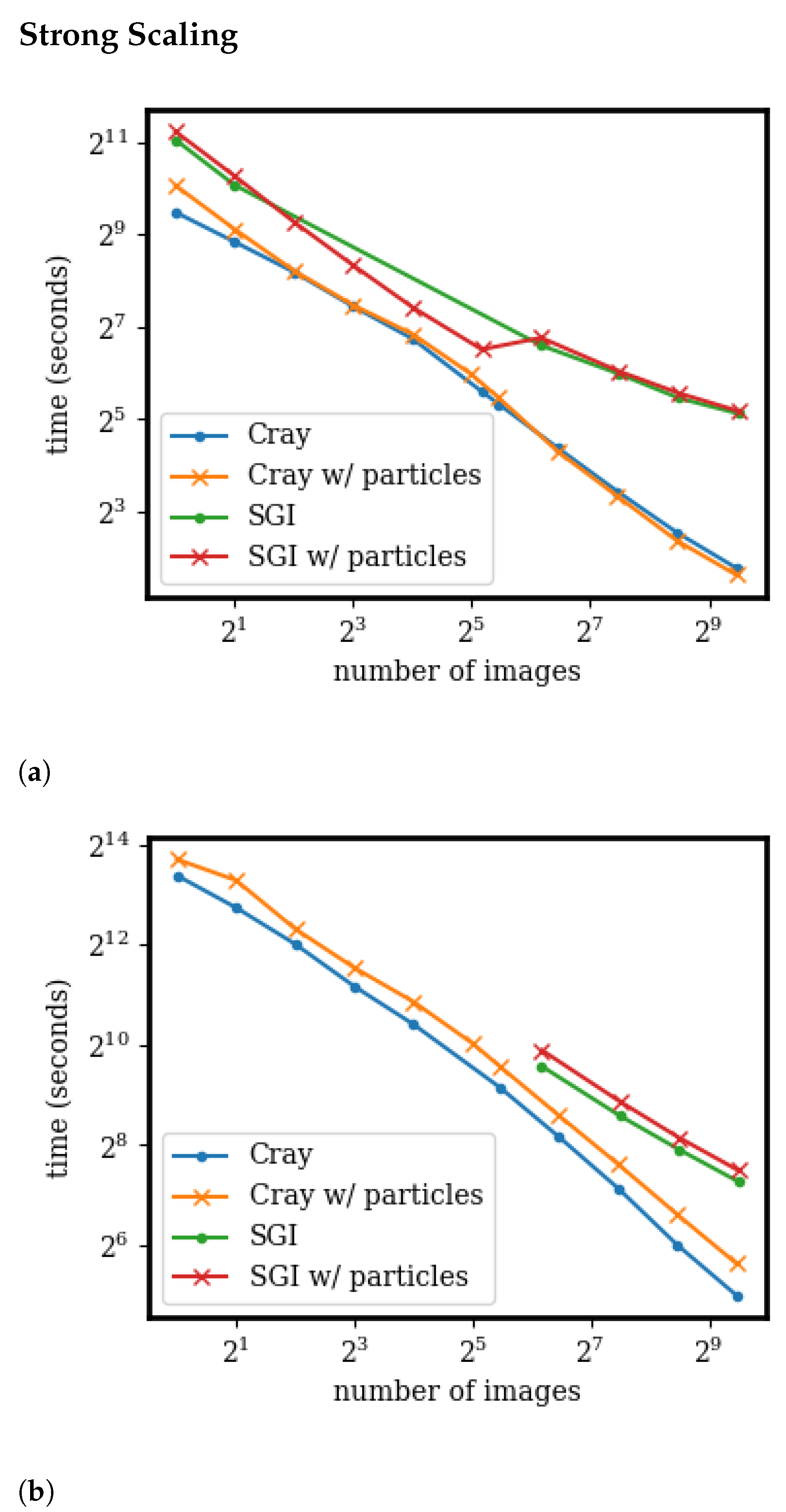
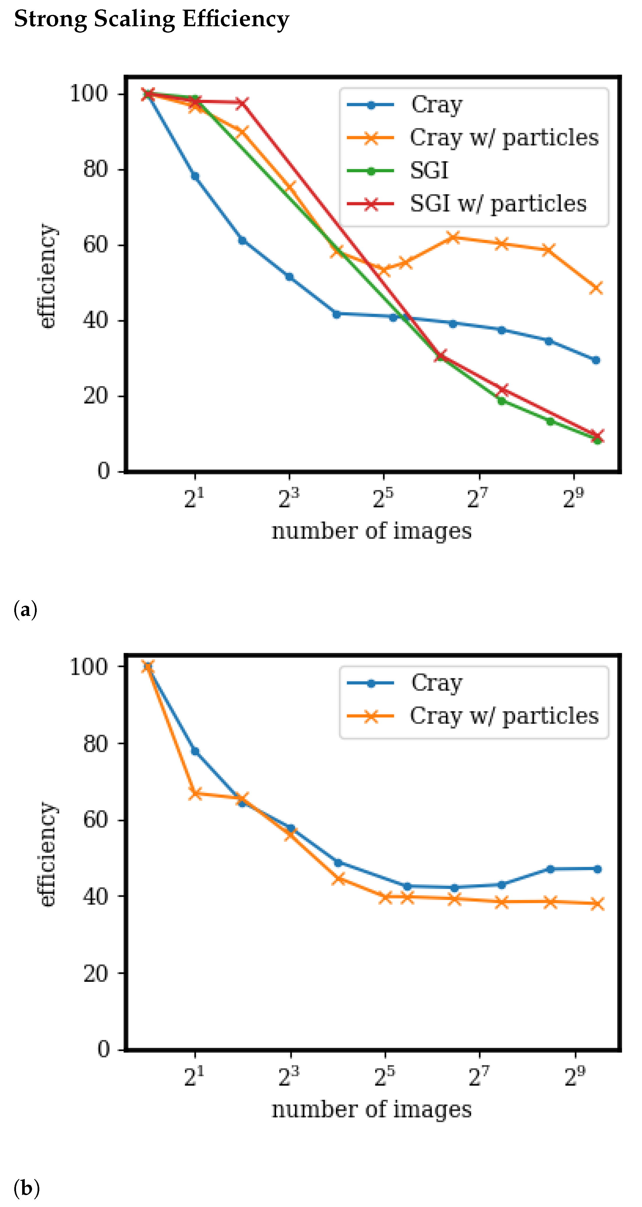
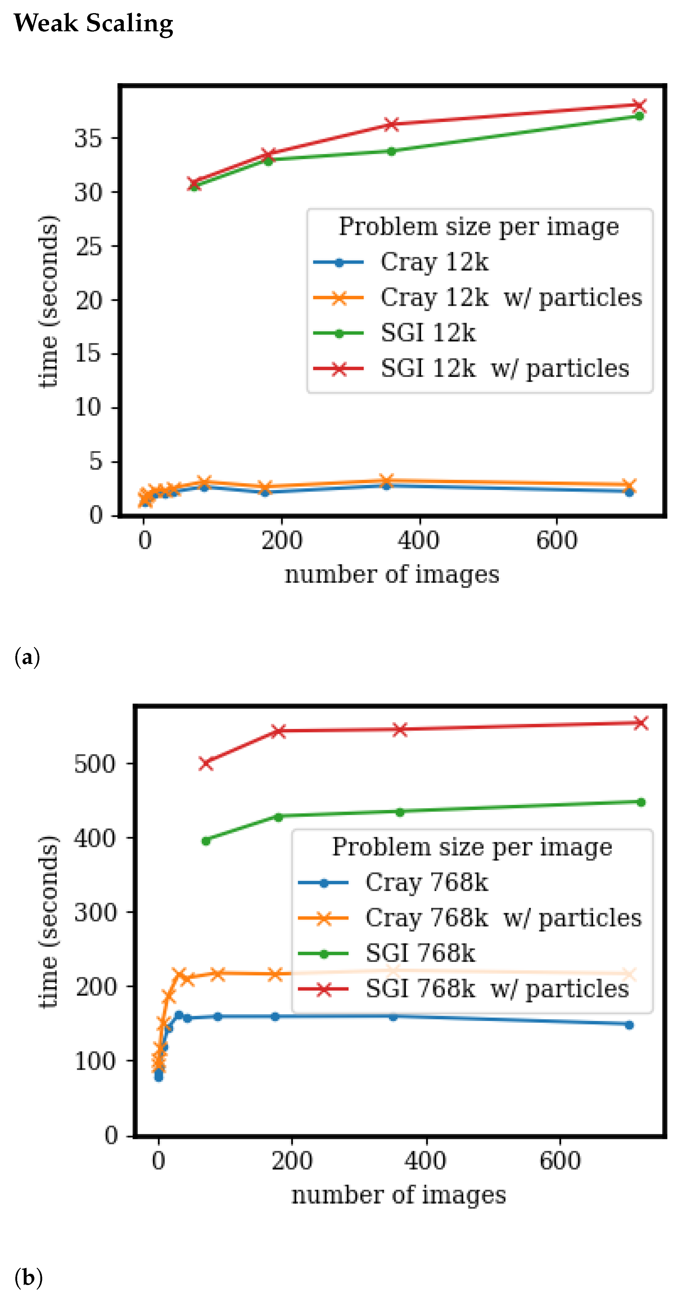
3.4. Scaling and Speedup
4. Conclusions
Author Contributions
Funding
Institutional Review Board Statement
Data Availability Statement
Acknowledgments
Conflicts of Interest
References
- Gutmann, E.; Barstad, I.; Clark, M.; Arnold, J.; Rasmussen, R. The intermediate complexity atmospheric research model (ICAR). J. Hydrometeorol. 2016, 17, 957–973. [Google Scholar] [CrossRef]
- Bernhardt, M.; Härer, S.; Feigl, M.; Schulz, K. Der Wert Alpiner Forschungseinzugsgebiete im Bereich der Fernerkundung, der Schneedeckenmodellierung und der lokalen Klimamodellierung. ÖSterreichische-Wasser-Und Abfallwirtsch. 2018, 70, 515–528. [Google Scholar] [CrossRef] [Green Version]
- Horak, J.; Hofer, M.; Maussion, F.; Gutmann, E.; Gohm, A.; Rotach, M.W. Assessing the added value of the Intermediate Complexity Atmospheric Research (ICAR) model for precipitation in complex topography. Hydrol. Earth Syst. Sci. 2019, 23, 2715–2734. [Google Scholar] [CrossRef] [Green Version]
- Horak, J.; Hofer, M.; Gutmann, E.; Gohm, A.; Rotach, M.W. A process-based evaluation of the Intermediate Complexity Atmospheric Research Model (ICAR) 1.0. 1. Geosci. Model Dev. 2021, 14, 1657–1680. [Google Scholar] [CrossRef]
- Numrich, R.W.; Reid, J. Co-Array Fortran for parallel programming. In ACM Sigplan Fortran Forum; ACM: New York, NY, USA, 1998; Volume 17, pp. 1–31. [Google Scholar]
- ISO/IEC. Fortran Standard 2008; Technical report, J3; ISO/IEC: Geneva, Switzerland, 2010. [Google Scholar]
- Coarfa, C.; Dotsenko, Y.; Mellor-Crummey, J.; Cantonnet, F.; El-Ghazawi, T.; Mohanti, A.; Yao, Y.; Chavarría-Miranda, D. An evaluation of global address space languages: Co-array fortran and unified parallel C. In Proceedings of the tenth ACM SIGPLAN Symposium on Principles and Practice of Parallel Programming, Chicago, IL, USA, 15–17 June 2005; pp. 36–47. [Google Scholar]
- Stitt, T. An Introduction to the Partitioned Global Address Space (PGAS) Programming Model; Connexions, Rice University: Houston, TX, USA, 2009. [Google Scholar]
- Mozdzynski, G.; Hamrud, M.; Wedi, N. A partitioned global address space implementation of the European centre for medium range weather forecasts integrated forecasting system. Int. J. High Perform. Comput. Appl. 2015, 29, 261–273. [Google Scholar] [CrossRef]
- Simmons, A.; Burridge, D.; Jarraud, M.; Girard, C.; Wergen, W. The ECMWF medium-range prediction models development of the numerical formulations and the impact of increased resolution. Meteorol. Atmos. Phys. 1989, 40, 28–60. [Google Scholar] [CrossRef]
- Jiang, T.; Guo, P.; Wu, J. One-sided on-demand communication technology for the semi-Lagrange scheme in the YHGSM. Concurr. Comput. Pract. Exp. 2020, 32, e5586. [Google Scholar] [CrossRef]
- Dritschel, D.G.; Böing, S.J.; Parker, D.J.; Blyth, A.M. The moist parcel-in-cell method for modelling moist convection. Q. J. R. Meteorol. Soc. 2018, 144, 1695–1718. [Google Scholar] [CrossRef] [Green Version]
- Böing, S.J.; Dritschel, D.G.; Parker, D.J.; Blyth, A.M. Comparison of the Moist Parcel-in-Cell (MPIC) model with large-eddy simulation for an idealized cloud. Q. J. R. Meteorol. Soc. 2019, 145, 1865–1881. [Google Scholar] [CrossRef] [Green Version]
- Brown, N.; Weiland, M.; Hill, A.; Shipway, B.; Maynard, C.; Allen, T.; Rezny, M. A highly scalable met office nerc cloud model. arXiv 2020, arXiv:2009.12849. [Google Scholar]
- Shterenlikht, A.; Cebamanos, L. Cellular automata beyond 100k cores: MPI vs. Fortran coarrays. In Proceedings of the 25th European MPI Users’ Group Meeting, Barcelona, Spain, 23 September 2018; pp. 1–10. [Google Scholar]
- Shterenlikht, A.; Cebamanos, L. MPI vs Fortran coarrays beyond 100k cores: 3D cellular automata. Parallel Comput. 2019, 84, 37–49. [Google Scholar] [CrossRef]
- Rasmussen, S.; Gutmann, E.D.; Friesen, B.; Rouson, D.; Filippone, S.; Moulitsas, I. Development and Performance Comparison of MPI and Fortran Coarrays within an Atmospheric Research Model. In Proceedings of the Workshop 2018 IEEE/ACM Parallel Applications Workshop, Alternatives To MPI (PAW-ATM), Dallas, TX, USA, 16 November 2018. [Google Scholar]
- Stein, A.; Draxler, R.R.; Rolph, G.D.; Stunder, B.J.; Cohen, M.; Ngan, F. NOAA’s HYSPLIT atmospheric transport and dispersion modeling system. Bull. Am. Meteorol. Soc. 2015, 96, 2059–2077. [Google Scholar] [CrossRef]
- Ngan, F.; Stein, A.; Finn, D.; Eckman, R. Dispersion simulations using HYSPLIT for the Sagebrush Tracer Experiment. Atmos. Environ. 2018, 186, 18–31. [Google Scholar] [CrossRef]
- Esmaeilzadeh, H.; Blem, E.; Amant, R.S.; Sankaralingam, K.; Burger, D. Dark silicon and the end of multicore scaling. In Proceedings of the 2011 38th Annual International Symposium on Computer Architecture (ISCA), San Jose, CA, USA, 4–8 June 2011; pp. 365–376. [Google Scholar]
- Moisseeva, N.; Stull, R. A noniterative approach to modelling moist thermodynamics. Atmos. Chem. Phys. 2017, 17, 15037–15043. [Google Scholar] [CrossRef] [Green Version]
- Stull, R.B. Practical Meteorology: An Algebra-Based Survey of Atmospheric Science; University of British Columbia: Vancouver, BC, Canada, 2018. [Google Scholar]
- Yau, M.K.; Rogers, R.R. A Short Course in Cloud Physics; Elsevier: Amsterdam, The Netherlands, 1996. [Google Scholar]
- Rasmussen, S.; Gutmann, E. Coarray ICAR Fork. [Code]. Available online: github.com/scrasmussen/coarrayicar/releases/tag/v0.1 (accessed on 14 January 2021).
- Rasmussen, S.; Gutmann, E. ICAR Data. [Dataset]. Available online: github.com/scrasmussen/icardata/releases/tag/v0.0.1 (accessed on 14 January 2021).
- Mandl, F. Statistical Physics; Wiley: Hoboken, NJ, USA, 1971. [Google Scholar]
- Marmelad. 3D Interpolation. Available online: https://en.wikipedia.org/wiki/Trilinear_interpolation#/media/File:3D_interpolation2.svg (accessed on 14 January 2021).
- University of Wyoming. Upper Air Soundings. Available online: weather.uwyo.edu/upperair/sounding.html (accessed on 10 November 2020).
- Sharma, A.; Moulitsas, I. MPI to Coarray Fortran: Experiences with a CFD Solver for Unstructured Meshes. Sci. Program. 2017, 2017, 3409647. [Google Scholar] [CrossRef] [Green Version]
- Fanfarillo, A.; Burnus, T.; Cardellini, V.; Filippone, S.; Nagle, D.; Rouson, D. OpenCoarrays: Open-source transport layers supporting coarray Fortran compilers. In Proceedings of the 8th International Conference on Partitioned Global Address Space Programming Models, Eugene, OR, USA, 6–10 October 2014; pp. 1–11. [Google Scholar]
- Feind, K. Shared memory access (SHMEM) routines. Cray Res. 1995, 53, 303–308. [Google Scholar]
- HPE Cray. Cray Fortran Reference Manual; Technical Report; Cray Inc.: Seattle, DC, USA, 2018. [Google Scholar]
- Shan, H.; Wright, N.J.; Shalf, J.; Yelick, K.; Wagner, M.; Wichmann, N. A preliminary evaluation of the hardware acceleration of the Cray Gemini interconnect for PGAS languages and comparison with MPI. ACM Sigmetrics Perform. Eval. Rev. 2012, 40, 92–98. [Google Scholar] [CrossRef]
- Shan, H.; Austin, B.; Wright, N.J.; Strohmaier, E.; Shalf, J.; Yelick, K. Accelerating applications at scale using one-sided communication. In Proceedings of the Conference on Partitioned Global Address Space Programming Models (PGAS’12), Santa Barbara, CA, USA, 10–12 October 2012. [Google Scholar]
- Shende, S.S.; Malony, A.D. The TAU parallel performance system. Int. J. High Perform. Comput. Appl. 2006, 20, 287–311. [Google Scholar] [CrossRef]
- Ramey, C.; Fox, B. Bash 5.0 Reference Manual. 2019. Available online: gnu.org/software/bash/manual/ (accessed on 12 May 2020).
- Kaufmann, S.; Homer, B. Craypat-Cray X1 Performance Analysis Tool; Cray User Group: Seattle, DC, USA, 2003; pp. 1–32. [Google Scholar]
- Zivanovic, D.; Pavlovic, M.; Radulovic, M.; Shin, H.; Son, J.; Mckee, S.A.; Carpenter, P.M.; Radojković, P.; Ayguadé, E. Main memory in HPC: Do we need more or could we live with less? ACM Trans. Archit. Code Optim. (TACO) 2017, 14, 1–26. [Google Scholar] [CrossRef] [Green Version]


| Nodes | Images | Time | Average Time (s) | Percent of Time | Average Time (s) | Percent of Time | Average Maximum |
|---|---|---|---|---|---|---|---|
| (s.) | PGAS | PGAS | __pgas_sync_all | __pgas_sync_all | Memory Usage (MBs) | ||
| 1 | 44 | 235.58 | 12.37 | 5.0% | 6.47 | 2.6% | 100 |
| 2 | 44 | 234.93 | — | — | — | — | — |
| 4 | 44 | 165.55 | 24.49 | 13.0% | 10.88 | 5.8% | 468.8 |
| 2 | 88 | 117.61 | — | — | — | — | — |
| 4 | 176 | 59.6 | — | — | — | — | — |
Publisher’s Note: MDPI stays neutral with regard to jurisdictional claims in published maps and institutional affiliations. |
© 2021 by the authors. Licensee MDPI, Basel, Switzerland. This article is an open access article distributed under the terms and conditions of the Creative Commons Attribution (CC BY) license (https://creativecommons.org/licenses/by/4.0/).
Share and Cite
Rasmussen, S.; Gutmann, E.D.; Moulitsas, I.; Filippone, S. Fortran Coarray Implementation of Semi-Lagrangian Convected Air Particles within an Atmospheric Model. ChemEngineering 2021, 5, 21. https://0-doi-org.brum.beds.ac.uk/10.3390/chemengineering5020021
Rasmussen S, Gutmann ED, Moulitsas I, Filippone S. Fortran Coarray Implementation of Semi-Lagrangian Convected Air Particles within an Atmospheric Model. ChemEngineering. 2021; 5(2):21. https://0-doi-org.brum.beds.ac.uk/10.3390/chemengineering5020021
Chicago/Turabian StyleRasmussen, Soren, Ethan D. Gutmann, Irene Moulitsas, and Salvatore Filippone. 2021. "Fortran Coarray Implementation of Semi-Lagrangian Convected Air Particles within an Atmospheric Model" ChemEngineering 5, no. 2: 21. https://0-doi-org.brum.beds.ac.uk/10.3390/chemengineering5020021