
Comprehensive Modeling of Vacuum Systems Using Process Simulation Software
by
 ,
,
Eduard Vladislavovich Osipov
* ,
,
Daniel Bugembe
,
Sergey Ivanovich Ponikarov
and
Artem Sergeevich Ponikarov
Machines and Apparatus in Chemical Production Department, Institute of Chemical and Petroleum Engineering, Kazan National Research Technological University, Karl Marx Street, 68, 420015 Kazan, Russia
*
Author to whom correspondence should be addressed.
ChemEngineering 2024, 8(2), 31; https://0-doi-org.brum.beds.ac.uk/10.3390/chemengineering8020031
Submission received: 19 January 2024
/
Revised: 18 February 2024
/
Accepted: 23 February 2024
/
Published: 6 March 2024
(This article belongs to the Topic Chemical and Biochemical Processes for Energy Sources)
Abstract
:Traditional vacuum system designs often rely on a 100% reserve, lacking precision for accurate petrochemical computations under vacuum. This study addresses this gap by proposing an innovative modeling methodology through the deconstruction of a typical vacuum-enabled process. Emphasizing non-prescriptive pressure assignment, the approach ensures optimal alignment within the vacuum system. Utilizing process simulation software, each component was systematically evaluated following a proposed algorithm. The methodology was applied to simulate vacuum-driven separation in phenol and acetone production. Quantifying the vacuum system’s load involved constructing mathematical models in Unisim Design R451 to determine the mixture’s volume flow rate entering the vacuum pump. A standard-sized vacuum pump was then selected with a 40% performance margin. Post-reconstruction, the outcomes revealed a 22.5 mm Hg suction pressure within the liquid-ring vacuum pump, validating the efficacy of the devised design at a designated residual pressure of 40 mm Hg. This study enhances precision in vacuum system design, offering insights that are applicable to diverse petrochemical processes.
1. Introduction
Modeling vacuum units in petrochemical installations is challenging due to the uncertainties in defining the key parameters. This arises from the complexity of characterizing all the contributing factors, resulting in a task lacking a clear structure. Established principles governing processes under atmospheric pressure undergo changes in a vacuum, revealing new patterns and characteristics.
The computational methodologies guiding the design of vacuum apparatus were explained in previous works [1,2,3,4]. The assessment of any vacuum system involves two crucial stages: the design phase and subsequent validation. During the design phase, decisions regarding the types of vacuum pumps are made, and the initial geometric parameters for the interconnecting pipelines among the key system elements are estimated [1]. The configuration of the vacuum system resembles analogous setups with a similar purpose, while the selection of the primary vacuum pump depends on the specified pressure thresholds, capacity requirements, and evacuation timelines.
The scientific literature contains numerous examples illustrating the calculation of technological processes that operate under vacuum conditions. For instance, in reference [5], factors influencing fuel–oil separation processes were outlined, while reference [6] explored ways to reduce the workload on the vacuum system based on the computational results. Reference [7] argued for the necessity of installing a fore-vacuum pump when modeling a membrane separation block, and reference [8] quantified the energy consumption of a vacuum pump during the purification process of butanol using hybrid membranes. Reference [9] investigated methods to reduce the boiling point differential in vacuum distillation, while reference [10] discussed the complexities of designing a Vacuum Distillation Unit (VDU).
The above-referenced articles heavily relied on process simulation software such as Aspen HYSYS (https://www.aspentech.com/en/products/engineering/aspen-hysys), Aspen Plus (https://www.aspentech.com/en/products/engineering/aspen-plus), and ChemCad (https://www.chemstations.com/CHEMCAD/) for conducting thermal and mass balance computations. However, when it came to the vacuum-based technological processes, the influence of the vacuum system was often overlooked, potentially compromising the accuracy of the modeling results. In reference [11], a specialized user module was incorporated into HYSYS to address this gap by computing steam ejector pumps, which are crucial in vacuum systems. Additionally, [12] emphasized that neglecting the intricacies of the technological process when modeling vacuum mixture condensation using such programs could introduce errors.
Traditionally, designers of vacuum systems and operational staff rely on industry experience when selecting the Vacuum Overhead System (VOS). However, during the design phase, there is often a lack of consideration for the specific requirements of the vacuum installation, leading to difficulties in achieving the desired residual pressure in the equipment.
The challenge of selecting the optimal VOS becomes apparent during comprehensive upgrades of technological installations due to the changes in the characteristics of the vacuumed object, rendering existing VOS specifications inadequate.
Therefore, designing a technological process under a vacuum requires simultaneous computations of the primary process within the technological object, the condensation block preceding the VOS, and the VOS itself. The complexity of designing and computing vacuum-based technological installations in chemical and petrochemical complexes lies at the intersection of vacuum technology and chemical engineering. Hence, this study aimed to devise a specialized methodology for modeling vacuum systems utilizing the capabilities of process simulation software. The developed methodology was intended for validation on a standard petrochemical installation, specifically targeting the waste separation block in phenol and acetone production.
2. The Conventional Approach to Designing Vacuum Systems
The traditional approach to designing vacuum generation systems involves calculating the overall gas flow entering the system and determining the effective pumping speed using Formula (1). Subsequently, the capacity of the vacuum pump is computed using Formula (2).
In Equations (1) and (2), p0—inlet pressure, Pa; —summary leak rate, m3·Pa/s; —required load on the VOS, m3/s; and —efficiency of the vacuum pump. The coefficient υ’s magnitude varies depending on the vacuum pump type and is referenced in specialized literature. For example, volumetric pumps hold a coefficient of 1.4, whereas jet pumps hold a coefficient of 2, indicating capacity margins of 40% and 100%, respectively [1,2,3,4].
The gas flow entering the evacuated object is calculated using Formula (3). In Equation (3), —represents the flow due to the permeability of the vacuum chamber walls, measured in m3∙Pa/s; —denotes the flow of atmospheric air entering the system, measured in m3∙Pa/s; signifies the gas flow resulting from the diffusion gas emission from the depth of structural materials and processed products, measured in m3∙Pa/s; indicates the gas flow from the surface of the working chamber and its components, measured in m3∙Pa/s; and represents the gas flow generated during the technological process, measured in m3∙Pa/s.
Industrial vacuum systems typically operate within pressure ranges of 0.5 to 500 mm Hg and exhibit temperatures ranging from 10 to 150 degrees Celsius. The gas release effects from constituent materials in these systems minimally impact the vacuum creation and maintenance processes in chemical-technological operations. Therefore, , , and can be neglected. Studies [12,13] demonstrated that leakage gas flows are not influenced by pressure but are mainly determined by temperature or equipment volume. Therefore, in Equation (3), (leak rate, m3∙Pa/s) can be replaced by (m3/s), resulting in Equation (4):
To estimate Vin, the empirical relationships outlined in [12,13] prove beneficial, whereas determining Vproc necessitates the construction of a computational model for both the block and the vacuum system (VS).
Current modeling and design tools for vacuum systems lack the requisite functionality to accurately compute Vproc. The methodologies embedded within vacuum Computer-Aided Design (CAD) systems are primarily devised for evacuating pristine air. Consequently, to attain the desired pressure, vacuum pump performance is often overstated by introducing performance safety margins.
Present-day advancements in process simulation software enable the calculation of Vproc, allowing for the potential abandonment of performance safety margins (or their reduction to an acceptable level). However, it is imperative to disassemble the vacuum block into its constituents and employ these software tools in a manner that accommodates the intricate interactions between the individual elements within the vacuum block.
3. Methodology for Coupled Modeling of Vacuum Blocks
The technological apparatus functioning under a vacuum presents a complex assembly, interlinking various apparatuses interconnected by technological streams. Processes involving chemical, petrochemical, or crude oil raw material processing under a vacuum can be deconstructed into key blocks:
- Main technological unit (or group of units) operating under vacuum;
- Vacuum condensers;
- Vacuum overhead system (VOS).
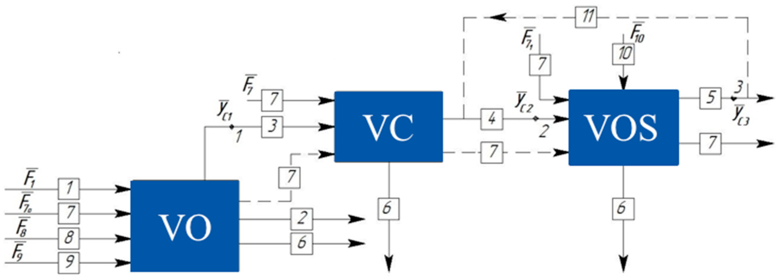
The vacuum block consists of diverse equipment, requiring separate energy resources (cooling water, steam, electrical power, etc.). Gases from leaks (atmospheric air) enter the system, and during the technological process, decomposition gases may be formed. Therefore, a typical vacuum chemical-technological installation can be represented as blocks shown in Figure 1 (solid lines depict the flows entering the system components).
In Figure 1, the following notations for streams are adopted: 1—raw material inlet; 2—product outlet; 3—non-condensable gases; 4—flow directed to the Vacuum Overhead System (VOS); 5—exhaust; 6—condensate; 7—energy resources; 8—decomposition gases; 9—ingress gases; 10—energy resource; 11—bypass flow facilitating VOS property regulation. Notably, points 1, 2, and 3 represent pivotal conjugation points.
The interconnected components of the examined VOS establish direct linkages via the gas pipelines housing the conjugation points: 1 (technological object pressure); 2 (VOS inlet pressure); and 3 (VOS exhaust). These junctures ensure equilibrium between the state parameters of the outgoing flows from the antecedent blocks and the incoming flows into the subsequent segments. If necessary, the recirculation of the energy resources or the flows between blocks can be organized. For example, the heat transfer fluid used from the previous block may be utilized in the subsequent one (stream 7), while a portion of the exhaust gas is returned to suction for regulating the performance of the VOS (stream 11). These connections are not always implemented in vacuum blocks; hence, they are depicted with dashed lines in Figure 1, Figure 2 and Figure 3.
The transformation of the input variable vector into output estimate vectors can be represented as a vector function . In this study, stands for the series of analytical or numerical (approximate) solutions to the system of equations that describe the chemical and technological processes within the equipment elements. refers to the coefficients within this system of equations .
In Equations (5)–(7), the indices to and correspond to the points indicated in Figure 1. The indices for relate to the streams specified in Figure 1 and represents the numerical values of the equations describing the chemical and technological processes within the equipment elements.
Given that the choice of vacuum pump relies on the volumetric flow rate of the mixture during suction, is established based on the dependence of the mixture’s volumetric flow rate on the intake pressure.
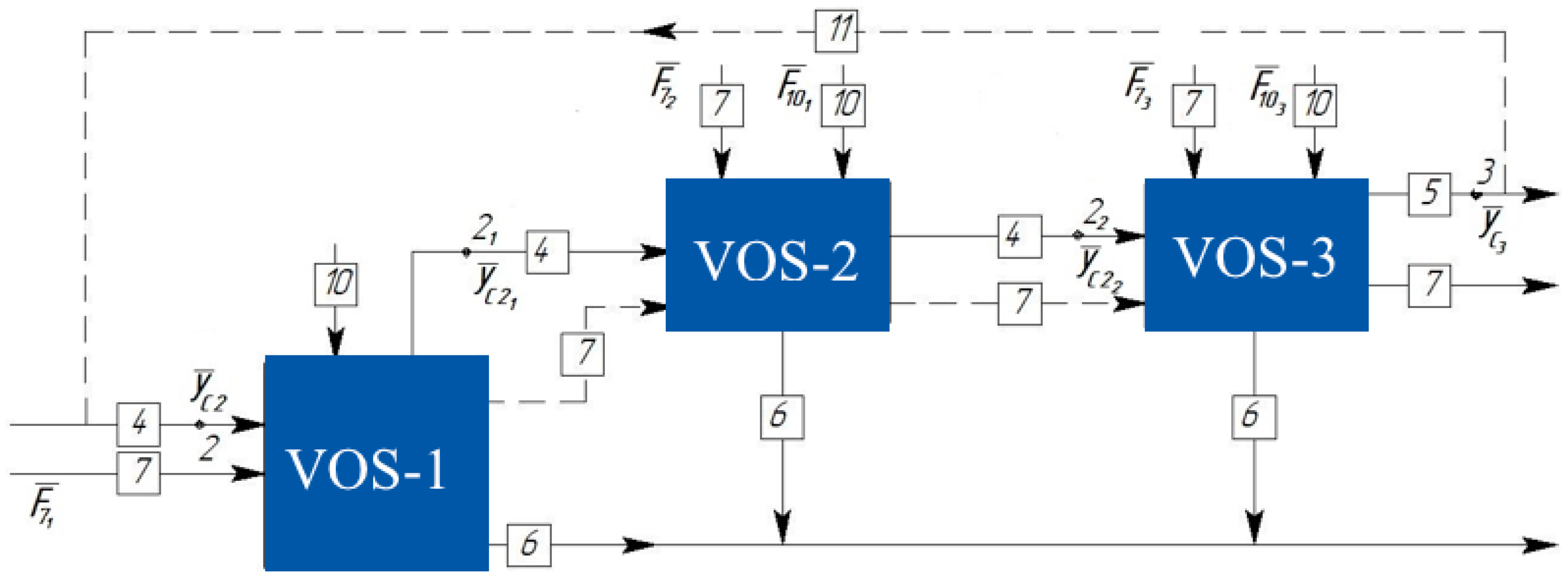
The Vacuum Overhead System (VOS) of an industrial chemical-technological process also consists of various equipment, allowing this block to be divided into a series of subsystems at one hierarchical level. If the VOS consists of three stages, the decomposition can be represented as shown in Figure 2.
Figure 2.
Decomposition of the Vacuum Overhead System (VOS) consisting of three blocks.

The additional conjugation points, identified as 21 and 22, arise from the interconnections among the constituent blocks, matching the number of linkages between the elements. Consequently, the vector functions governing the intricate chemical-technological system operating under vacuum, comprising a VOS with three blocks, can be formulated as follows:
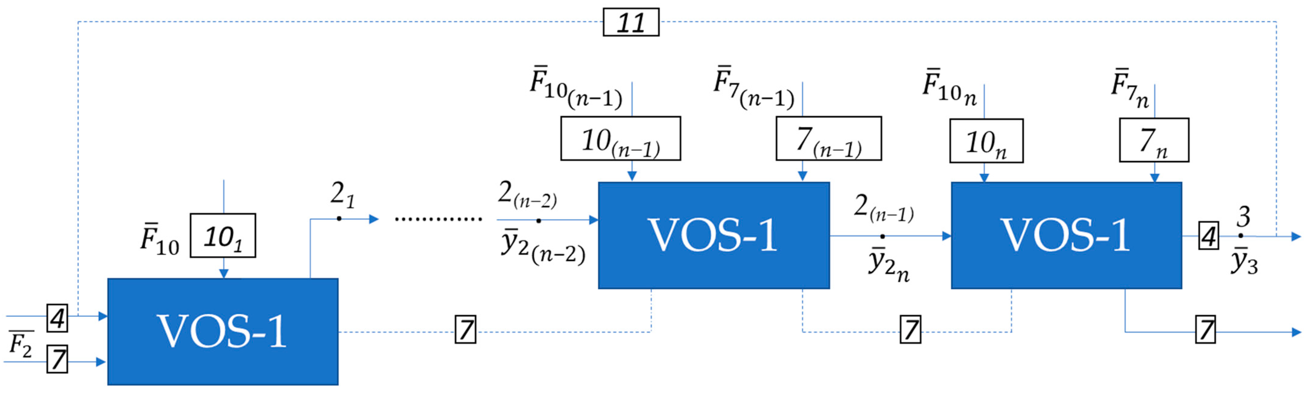
If the VOS consists of n (n = 1, …, N) blocks, then the decomposition of the system will take the form shown in Figure 3.
![Chemengineering 08 00031 g003]()
Figure 3.
Decomposition of a VOS consisting of n blocks. The vector functions of the constituent elements of a vacuum overhead system consisting of n elements will be written as follows:
Figure 3.
Decomposition of a VOS consisting of n blocks. The vector functions of the constituent elements of a vacuum overhead system consisting of n elements will be written as follows:

In this context, the vector function representation for the first element (stage) of the VOS would resemble Equation (1).
Characterizing the components of the CVCTS (Complex Vacuum Chemical Technology System) facilitates the calculation of the thermal and mass balances of the installation and addresses synthesis and optimization tasks.
The alignment of properties between the technological object and the vacuum creation system implies the coordination of their fundamental characteristics. By fundamental characteristics, we mean the key parameters describing the operating conditions of these blocks as a unified whole.
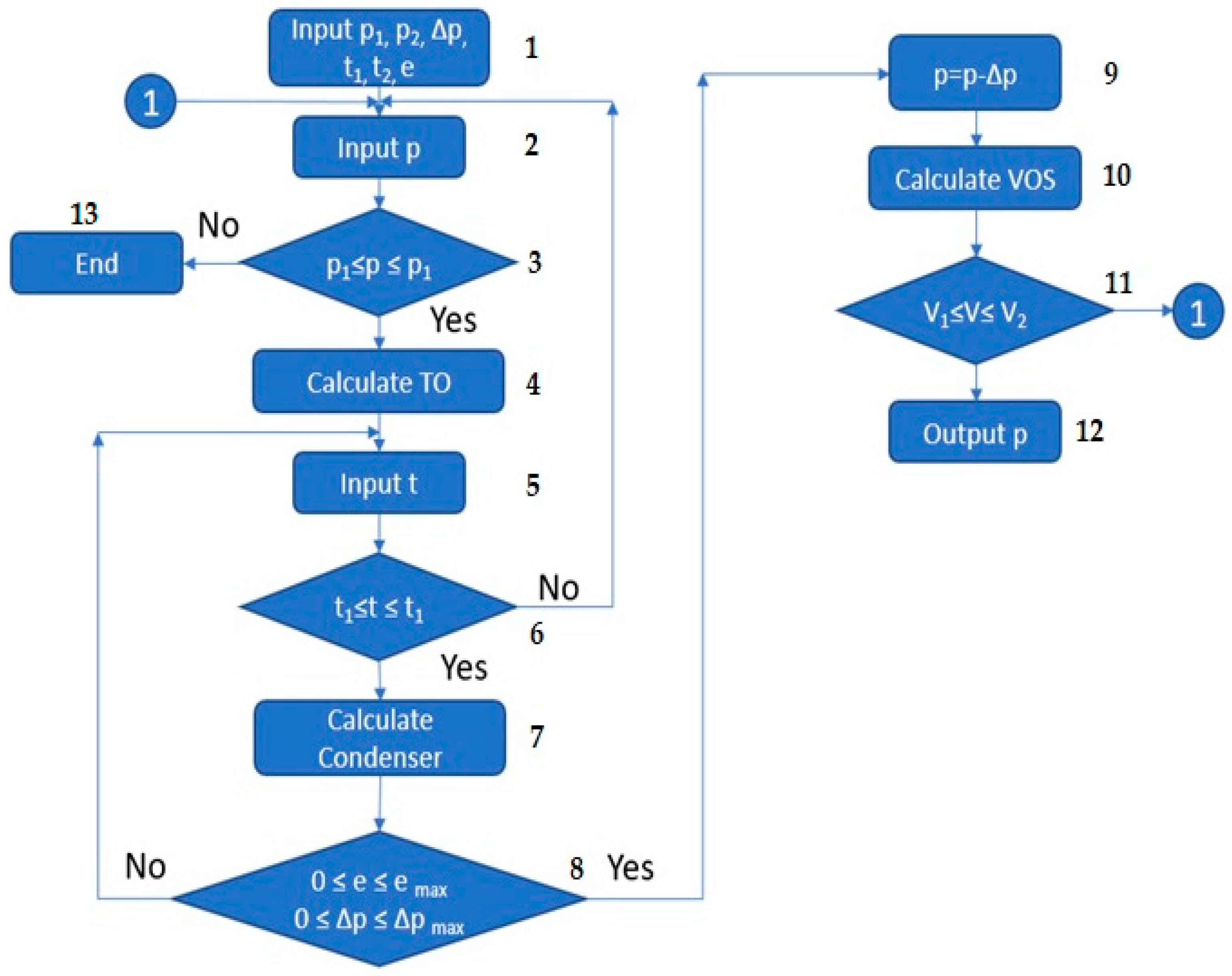
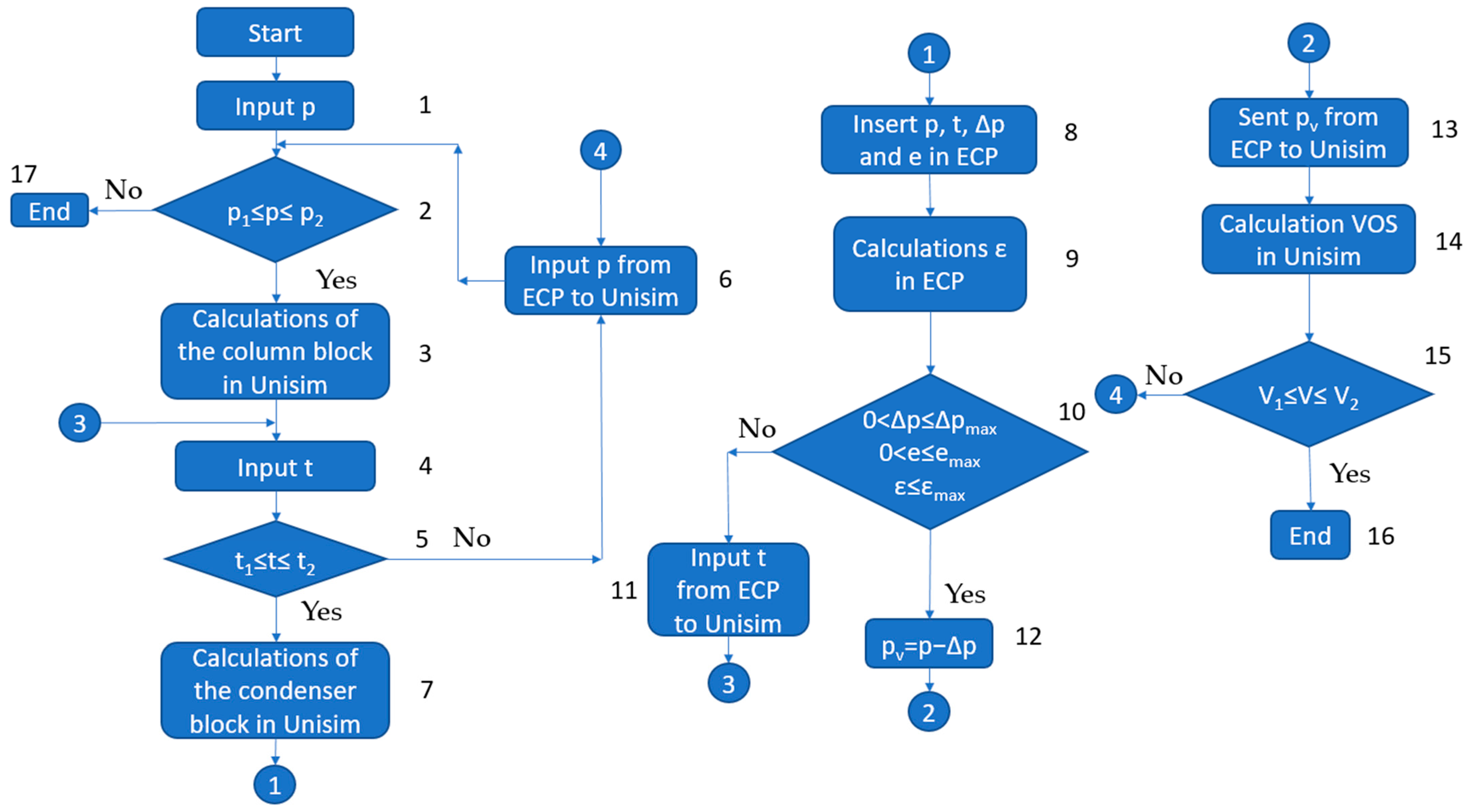
Interconnecting the elements within the vacuum block is envisaged based on the block diagram depicted in Figure 4. Opposite each symbol in the flowchart is the step number, and the description is provided below.
- Introduce the minimum and maximum possible pressures in the object (p1 and p2, respectively), the minimum and maximum temperatures in the condenser (t1 and t2, respectively), the allowable pressure drop Δp, and the heat exchange surface margin e (0 < e ≤ 5%);
- Set the initial value of the pressure p in the vacuumized technological object;
- If the condition p1 ≤ p ≤ p2 is met, proceed to step 4;
- Calculate the vacuumized technological object and determine the parameters of the flow entering the condenser (or group of condensers);
- Introduce the initial approximation of the cooling temperature of the mixture, t;
- If the condition t1 ≤ t ≤ t2 is met, proceed to step 7. If the condition is not met, assign a new value of pressure to the technological object (step 2);
- Calculate the condenser and determine the load on the VOS;
- If the heat exchange surface margin and pressure drop do not exceed the specified values, proceed to the next step. Otherwise, assign a new value to t (repeat step 5);
- Assign the pressure at the VOS inlet, which is less than the pressure in the technological object by the pressure drop in the condenser Δp;
- Calculate VOS;
- If the recorded performance of VOS is greater than the volumetric flow rate at the condenser outlet (V1) and does not exceed the maximum permissible performance (V2), proceed to step 12. If this condition is not met, assign a new pressure to the technological object (step 2);
- Fix the pressure in the technological object and conclude the calculation;
- If, in the end, the pressure in the technological object satisfies all the specified conditions, the calculation is completed, and it is concluded that the specified VOS is not suitable for the investigated process.
The introduced maximum and minimum values of the pressures and temperatures, pressure drop, and heat exchange surface margin at the first stage depend on the characteristics of the technological equipment and the type of chemical-technological processes taking place in it. For instance, the cooling temperature of the mixture (t) depends on the initial and final temperatures of the coolant. If the temperature of the refrigerant at the condenser inlet is 28 °C, and at the outlet is 38 °C, then the temperature t cannot be lower than 39 °C [5,6]. Meanwhile, the maximum temperature (t2) is approximately 50–60 °C since at higher temperatures, the condensation of the mixture would be insufficient [10,11]. Additionally, if the rear end head types are L or M (according to standards [14]), the allowable temperature difference between the wall and the jacket cannot exceed 40 °C.
Maximum and minimum pressures are determined by the norms of the technological regime. For rectification processes, the pressure is chosen to eliminate product decomposition in cubic sections (or in the furnaces of the preheating raw materials) [5] while reducing energy input. When conducting vacuum condensation, the pressure drop should be minimal [5,6].
The proposed approach for modeling vacuum blocks is only feasible with an accurate calculation of the technological object, condensation block, and VOS. Present vacuum system design tools [15,16] lack the functionality to compute the technological components of petrochemical installations. Therefore, process simulation software is recommended for this purpose.
In process simulation software, a mathematical model of blocks is constructed, comprising interconnected modules selected from the program’s database. Assigning temperatures and pressures is executed through a developed external control program. This program includes an algorithm, depicted in Figure 4, utilizing calculated heat and physical parameters of flows as input data from the process simulation software and providing the temperature within the condensation block and the pressure in the object as output data.
The program is designed to load the required flow parameters from the calculated Process Flow Diagram (PFD) of the process:
- Pressures in the technological object;
- Temperatures in the condenser;
- Volumetric flow rate of the mixture at the condenser outlet;
- Pressures in the condenser;
- Heat exchange surface margin of the condenser;
- VOS performance.
The program checks the conditions of steps 3, 6, 8, and 11. If any of the conditions in the flowchart (Figure 4) are not met, the user inputs a new temperature or pressure value into the program, which is then loaded into the corresponding modules of the process simulation software. The PFD is initiated for calculation, and the calculated values of e and Δp are loaded back into the program. The execution of steps 12 and 13 is determined by the user and depends on the required temperature and pressure ranges. The program is written in VBA using recommendations [17,18].
4. Description of the Research Object
The research subject chosen was a vacuum block for processing phenol and acetone waste, representing a typical petrochemical installation operating under vacuum conditions. The vacuum overhead system in the distillation unit for the separation of phenol and acetone products is typically equipped with steam ejection units [23,24]. Despite their simplicity of design and ease of operation [5], steam ejection units exhibit several significant drawbacks, the most prominent of which is their low thermodynamic efficiency and consequent high energy consumption. Moreover, when the working agent condenses in the inter-stage barometric condensers of the steam ejection units, the distillate components from the pumped gas co-condense, leading to a mixture of distillate products and condensate from the working water vapor. Consequently, the condensate from vacuum overhead systems is unsuitable for reuse in power plants and must be treated as chemically contaminated water, incurring additional costs.
High-potential superheated water vapor acts as a working agent in steam ejection units, with the residual pressure reached by the pump determined by its temperature, pressure, and flow rate. It is worth noting that the parameters of the technological approach, including the operating pressure sustained in the vacuum columns, deviate considerably from those specified in the project. Therefore, the steam ejector pumps operate below their calculated modes, leading to a further decrease in their efficiency.
Replacing steam ejector vacuum pumps with an environmentally friendly hydro-ejection Vacuum Overhead System (VOS) is a crucial task to reduce energy consumption and minimize pollutant emissions.
The waste processing rectification unit in the main phenol–acetone production incorporates a hydrocarbon fraction processing unit aimed at the extraction of isopropylbenzene (IPB) and alpha-methylstyrene (AMS). This unit consists of six distillation columns, with five of them operating under vacuum conditions.
The Complex Chemical Technological System (CCTS) comprises several key components, including vacuum distillation columns (VC), condensation units (CU), vacuum overhead systems (VOS), and transfer pipelines (TP) connecting the VC, CU, and VOS. The efficiency of the system is heavily influenced by the performance of these pipelines, which affect the vacuum pressure attained within the rectification column and thus the properties of the entire CCTS. Given the system’s integrative nature, it is impossible to analyze the individual components in isolation from the conjugate elements. Modeling tools such as Unisim Design R451, designed to simulate a broad range of chemical processes and devices including rectification systems, provide an effective means of studying such complex systems.
Schematically, the plant for processing waste from the production of phenol and acetone is shown in Figure 5 [24].
In the initial phase, an examination of the current operating conditions of the distillation columns, namely K-4, K-31, K-37, K-48, and K-58, was conducted. The primary aim of this survey was to establish the technical mode parameters of the process, which would be employed as inputs for the mathematical model of the block. Particular attention was paid to measuring the temperatures and pressures of the pumped gases along the path from the distillation column to the vacuum overhead system. These data were deemed critical for the successful completion of the survey.
Sampling points were chosen at each installation to measure pressure as close as possible to the outlet of the steam–gas mixture from the distillation column (helmet line), the first and second stages of dephlegmation, and the entrance to the suction pipe of the Steam Ejector Pump (SEP), where feasible. The measurement locations of the analyzed parameters were coordinated with the technical service department of the plant. Pressure measurements were carried out using a model vacuum meter that was verified metrologically and met the required measurement accuracy. The measured parameters were compared with the data of technological regulations and indications of stationary measuring devices in the production environment. The results of the survey are presented in the table.
Upon analyzing the results presented in Table 1, it can be inferred that the vacuum overhead system (VOS) of the K-31 and K-48 columns is operating in the overload region. This is attributed to the high condensation temperature of the condensation unit [25]. Additionally, the maximum residual pressure developed by the VOS depends on the gases that are not condensed in the condensation unit. These uncondensed vapor–gas mixtures (VGMs) are formed due to the thermal decomposition of the cubic product and the entry of “flow gasses” like atmospheric air into the system, as any evacuated system will receive an external environment to some extent through micro-densities such as welds, gaskets, pump seals, etc. Although the amount of leakage gases is relatively small, it cannot be ignored in this case, as they significantly influence the load on the evacuation unit (VOS).
5. Description and Validation of Simulation Model of the Block
According to recommendations [17,26,27], for calculating VLE, one can use the Wilson model, UNIQUAC, and NRTL.
The Wilson equation is more complex than the van Laar or Margules equations and requires more processor time [17]. However, it satisfactorily represents nearly all non-ideal liquid solutions, except for electrolytes and solutions demonstrating limited miscibility. The Wilson equation provides similar results to the Margules and van Laar equations for weak non-ideal systems but consistently outperforms them for increasingly non-ideal systems.
NRTL is an extension of the Wilson equation [28]. It uses statistical mechanics and liquid cell theory to represent the liquid structure. It is recommended for highly non-ideal chemical systems and can be used for VLE and LLE applications.
UNIQUAC uses statistical mechanics and the quasi-chemical theory of Guggenheim to represent the liquid structure [29]. The equation is capable of representing LLE, VLE, and VLLE with accuracy comparable to the NRTL equation, but without the need for a non-randomness factor.
During the production of phenol and acetone using the cumene method, phenol tar is formed [30]. This complex material comprises various components, including phenol, acetophenone (AP), α, α-dimethylbenzylalcohol (DMBA), dimers of α-methylstyrene (AMSD), o, p-cumylphenols (CP), unidentified components, and a small number of salts (mainly Na2SO4). The exact composition of phenol tar depends on the specific phenol production technology and can vary widely. The composition of phenol tar is not determined in the considered production process, which complicates the characterization of the feed stream and PFD setup.
Since the phenol tar component is not available in the program’s database, it was created based on the p-cumylphenol component.
To use the NRTL model, the parameter cij needs to be inputted, and the recommended values depend on the type of mixture. Due to the presence of the phenol tar component, it was challenging to select this value, so the decision was made to try using the UNIQUAC model. However, during the calculation of columns K-4 and K-58, convergence was not achieved. These columns were only calculated using the Wilson model, where the parameter aij had to be adjusted to match the production data in terms of the flow rate, composition, and temperature of cube K-4. The thermodynamic model used for the vapor phase is the Ideal Gas law.
The model is based on the Equations (12)–(14):
Once the fluid package and the component list are defined, the parameters used are the ones set as default by the software database, as presented in Table 2. It is to be stressed that such values have not been modified, i.e., Equations (12)–(14) are solved with the numbers in Table 2. The parameter was assumed to be equal to 0.
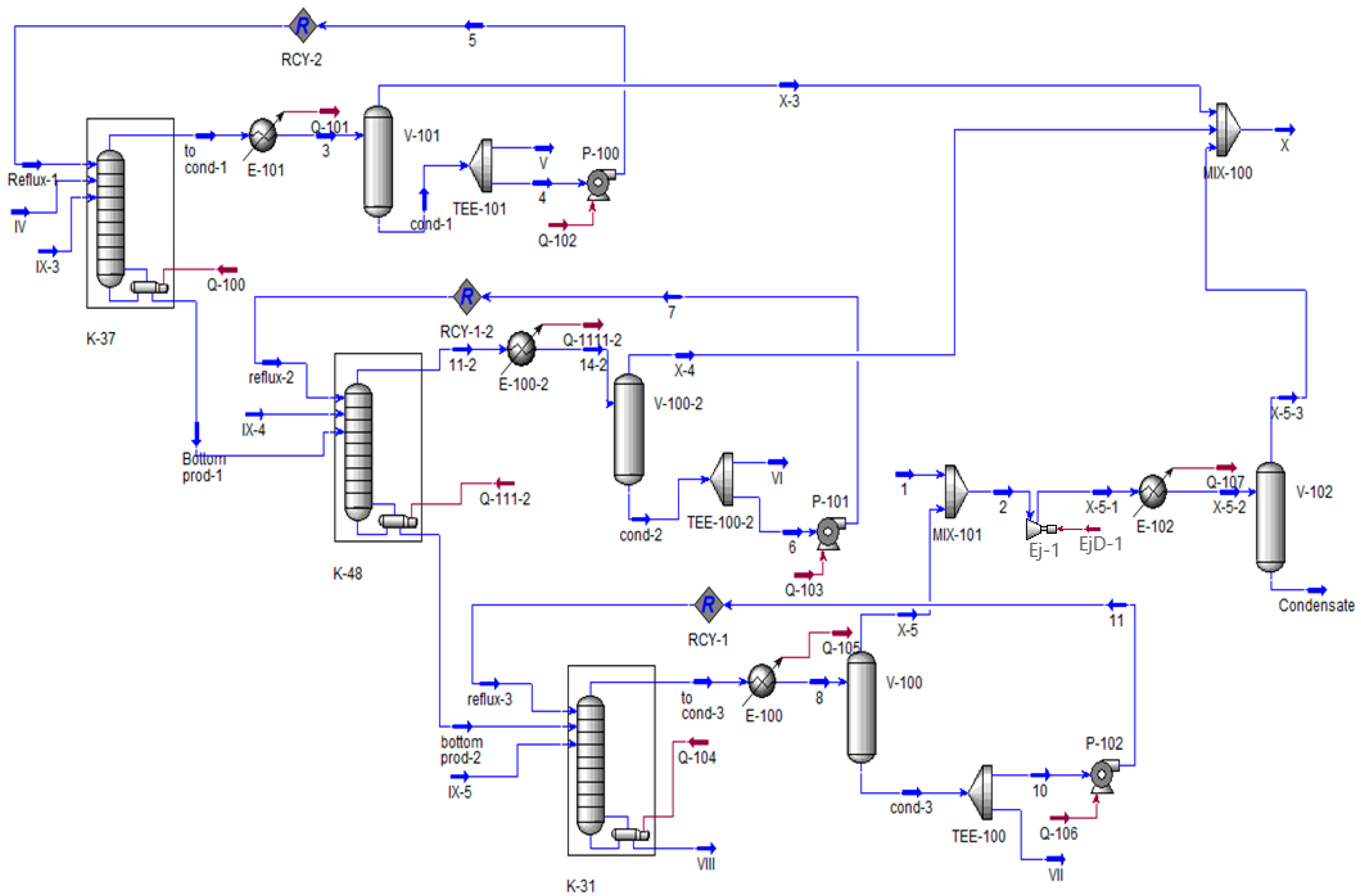
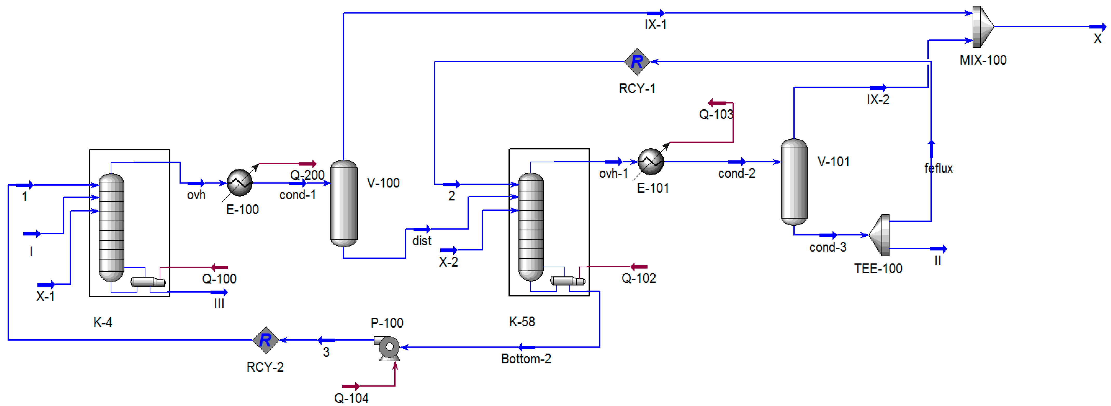
Further, calculation models of vacuum columns were synthesized in the Unisim Design R451 software package, in which the data of the technological survey were set as specifications. The calculation schemas of the block are shown in Figure 6 and Figure 7.
In Figure 6 and Figure 7, the designations are identical to Figure 5, except for stream X, which simulates the intake of atmospheric air into the evacuated objects.
The results of comparing the calculated data with the results of the industrial survey are presented in the tables below.
For a better assessment of Table 3 and Table 4, calculated overall and component balances based on the Process Flow Diagrams of Figure 6 and Figure 7 are presented in the
Appendix A.
In Table 3 and Table 4, the values of temperatures and flow rates calculated by the models are in good agreement with the production data. The contents of the main (target) components in the flows also match the technological regulations (deviation is not more than 10%). The content of auxiliary components (non-target) may deviate up to 100% but their total content in the flows does not exceed five (mass%), which does not significantly affect the accuracy of the calculation. Based on Table 3 and Table 4, it can be concluded that the calculation results for the streams denoted with an asterisk (*) are in close agreement with the corresponding data obtained from the survey (streams without an asterisk). This observation indicates that the mathematical model developed for the process is sufficiently accurate and reflects the actual technological process being studied.
The temperature of stream I set in the program (140 °C) differs from the industrial one because the conditions are maintained at the plant to ensure that the inlet stream I does not overheat above 150 °C. Typically, the operating personnel maintain the temperature at around 140 °C; therefore, this value was chosen as the input parameter.
6. Selection of a Vacuum Overhead System
The circumstances outlined led to the proposal to revamp the vacuum overhead system (VOS) across all the distillation columns within the unit. The aim was to replace the existing steam ejector pumps (SEP) with a new generation of energy-efficient and environmentally friendly VOS. This transition seeks to reduce operational expenses related to establishing and maintaining vacuum levels while also minimizing the production of chemically contaminated effluents.
Innovative hydro-circulatory VOS designs have been developed and implemented in the industry, utilizing either single-stage liquid ejectors (LE) or liquid-ring vacuum pumps (LRVP) as operational mediums, with distillates from the distillation columns being used in both cases. Previous analyses demonstrated that a VOS relying on LRVP demonstrates better cost-effectiveness in terms of both SEP and VOS operational expenses within the vacuum range of 50 mm Hg and higher compared to a VOS relying on LE. This observation also extends to capital investments, which is crucial given the need to ensure VOS redundancy for the secure operation of these facilities, considering the intricacies of vacuum rectification technology.
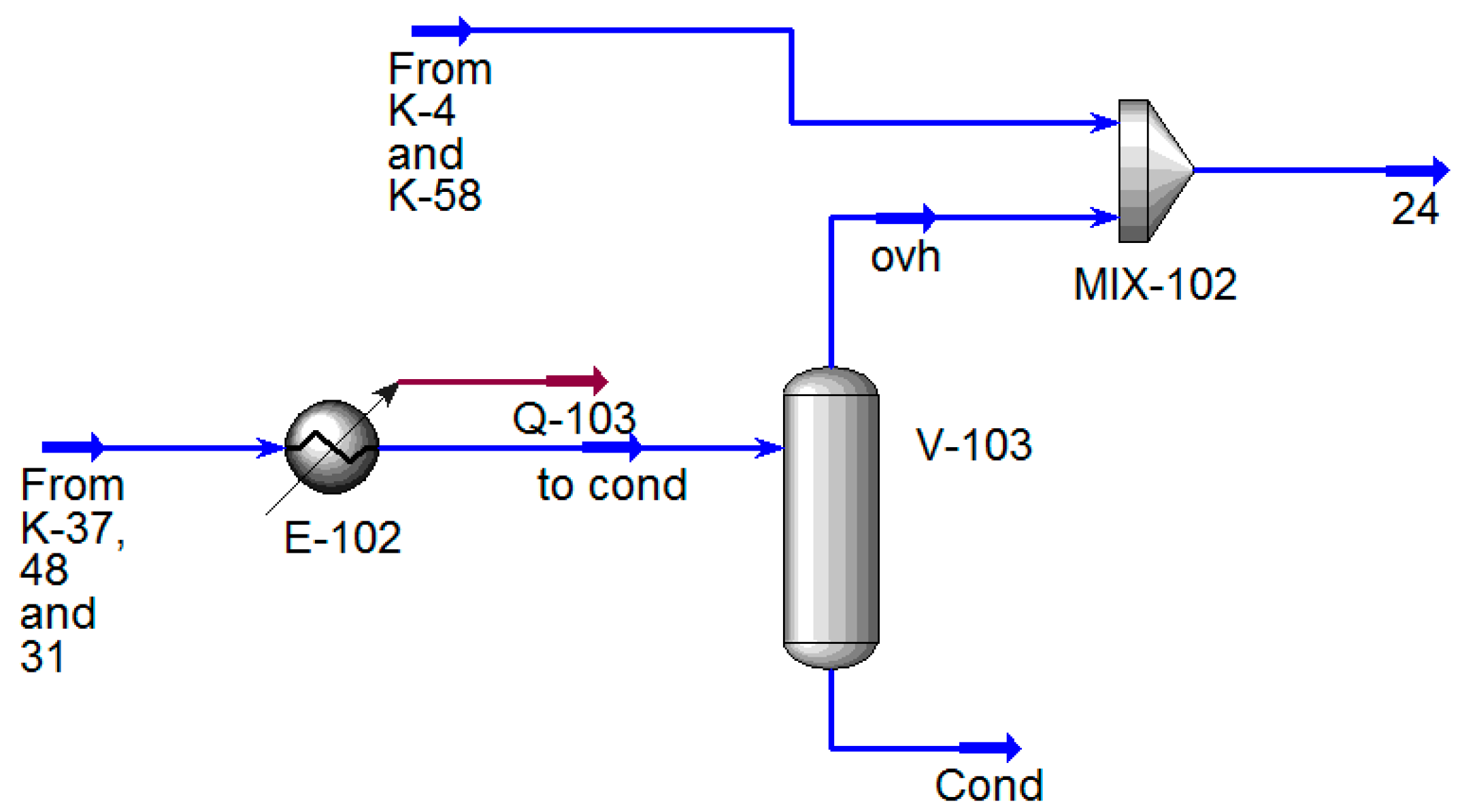
A conceptual proposal for the reconstruction involves the implementation of a hydro-circulatory single vacuum-generating station employing a liquid-ring vacuum pump (LRVP). Figure 8 illustrates the block diagram depicting the envisioned reconstruction plan for the vacuum block.
Figure 8 depicts the block diagram of the proposed reconstruction of the vacuum block, where the stream designations are similar to those in Figure 5, except for stream XI, which represents the condensate stream formed in a condenser installed at the outlet of the uncondensed gases from columns K-37, 48, and 31. As recommended in [31,32,33,34,35], the vacuum-generating system must be selected based on the required load. A LRVP with a capacity of 610 m3/hour was chosen as the VOS. The parameters and composition of the pumped mixture were calculated according to the models of Figure 2 and Figure 3 and are presented in Table 5.
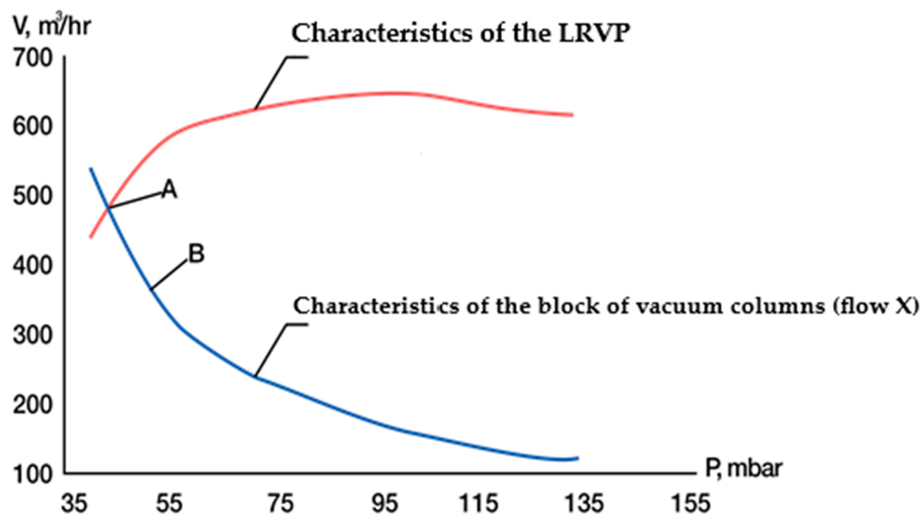
The pairing of the characteristics of a group of coupled columns and the standard characteristics of the LRVP are presented in Figure 9.
It was observed that the characteristics of these elements intersect at point A, which corresponds to a pressure of 33 mm Hg (43.89 mbar). Due to the limited accuracy of modeling the hydraulic resistance of the gas path and condensing units, the system pressure was adjusted to 40 mm Hg (53.2 mbar) using anti-surge protection of the pump at point B.
In light of the results obtained, it can be concluded that the LRVP utilized in this CCTS operates with a 40% productivity margin at the working point. This margin serves to mitigate the potential impact of temperature increases in the condensation units that may occur during the summer operating period of the installation.
7. Connection of the VOS to the Reconstructed Unit
Upon completion of the reconstruction, the start-up of the vacuum system was conducted in a specific sequence:
- Initially, all column sections were transitioned to operate at the recommended mode with a pressure of 40 mm Hg, using regular SEPs to establish the vacuum;
- Subsequently, the LRVP P2L 65327 Y 4B was launched via a separately mounted communication in parallel with the existing SEP. As the anti-surge system automatically activated, the vacuum pressure in the system remained largely unaffected;
- Following this, at intervals of 10–15 min, the SEPs were turned off for all columns, except for the K-31 column, while maintaining the pressure at the prescribed level. The entire system restart process did not exceed 1 h.
The K-31 column experienced a pressure of 55 mm Hg, surpassing the design value of 40 mm Hg. This deviation likely stemmed from the inadequate performance of the column’s condensation unit, resulting in a condensation temperature exceeding 60 °C, along with significant hydraulic resistance in the condenser. As a result, the column failed to achieve the required separation efficiency. To rectify this issue, a standard steam ejector pump with a barometric condenser was installed downstream of K-48, effectively reducing the column’s pressure to the target value of 40 mm Hg. It is important to note that phenolic water with a phenol concentration of up to 4% by weight was utilized as the working fluid, necessitating recalibration of the pump’s characteristics based on the methodology outlined in [36,37], or the model presented in [38]. To mitigate potential calculation inaccuracies, a 40% performance margin was incorporated to enhance the modeling of the system’s bottlenecks. This approach proved effective overall, except for the K-31 column, where the issue of high condensation temperature in the condensation unit persisted.
8. Coupling of the Characteristics of the VOS and the Vacuum Unit, Taking into Account the Operating Conditions
The utilization of the methodology and thinned models of an LRVP [38] can provide a means to manage the selected stock coefficients and enhance the effectiveness of the proposed design solutions. Therefore, recalculating the block of distillation columns to suit new production conditions and coupling their characteristics with the recalculated characteristics of the selected LRVP would be of significant scientific and practical interest.
Subsequently, a technological survey was conducted to gather temperature data at the top and bottom of vacuum columns, as well as reflux rate costs, after the completion of the reconstruction project of the vacuum-generating system for the separation of the rectification of phenol and acetone production waste. These data were crucial for establishing a mathematical model and verifying its adequacy.
It should be noted that during the reconstruction and replacement of the vacuum overhead system for improved vacuum creation, various modifications were implemented, including the installation of an additional condenser before the LRVP, the use of salted brine (a mixture of water with 5% mass phenol) instead of water, and changes in the pipelines connecting the column condensers with the vacuum overhead system. As a result, not only did the operating parameters of the system change, but the technological topology was also altered.
Consequently, the previously developed models, as presented in Figure 6 and Figure 7, became unsuitable and required additional modifications. To this end, the models in Figure 6 and Figure 7 were updated with the addition of blocks for mixing the streams of uncondensed gases that were suctioned at the VOS, and a block for cooling and condensing the streams of gases leaving the K-37, 48, and K-31 columns was also included.
The modification involved adding a model for the first stage SEP to column K-48 (Figure 10) following the recommendations [39]. The parameters for the stage were adopted based on the data from [40]. As a result of these modifications, the models of the columns and the condensation unit had to be updated, which can be observed in the modified versions presented in Figure 10, Figure 11 and Figure 12.
The temperature in the inter-tube space has a significant impact on the point of conjugation between the characteristics of the vacuum column and the vacuum overhead system. To account for this, temperature data were incorporated into the specifications of the cooler modules in Unisim Design R45. The temperature values were determined through a technological survey and used to obtain accurate results.
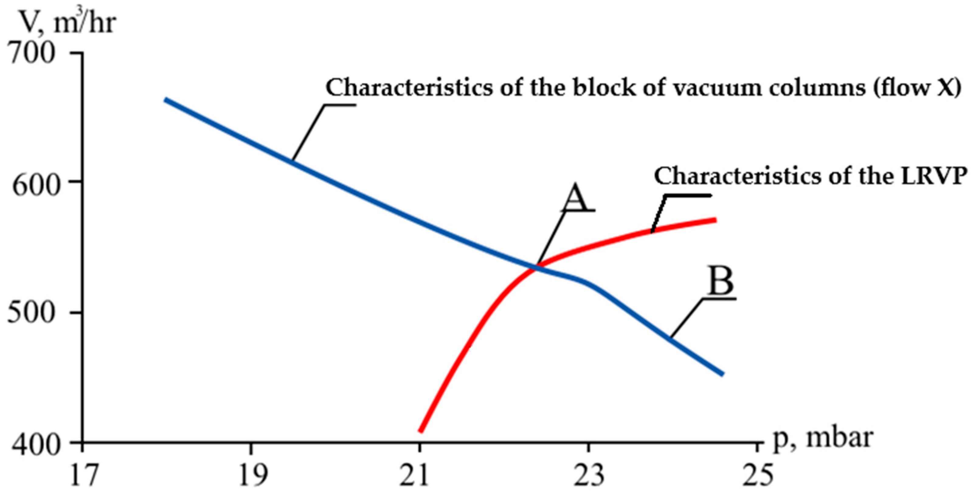
As noted previously, a characteristic feature of volume flow is its dependence on pressure. The characteristics of the vacuum distillation column unit are defined by the output of the uncondensed vapor phase in the condensation units, whereas for the vacuum overhead system, the corresponding characteristic is the input stream at the inlet of the vacuum pump. The points where these characteristics intersect can be referred to as conjugate points.
Simulation flowchart VO and VOS are shown in Figure 13. The conjugate points of the block of rectification columns and the VOS were determined using the following method:
- At the initial stage, an initial pressure approximation is introduced into the columns;
- If the pressure falls within the specified range, the calculation proceeds. If not, the calculation is terminated and it is considered that the VOS is not operational in this production;
- The columns are calculated in the Unisim software package;
- The initial temperature value in the condensers is introduced;
- The condition that the temperature value must lie within the range specified in Table 6 is checked. If the condition is met, the calculation continues (step 7);
- If the condition is not met, a new pressure value is introduced via the specially developed ECP, and the calculation starts again from step 1;
- The condensation block is calculated in the Unisim software package;
- The values of p, t, Δp, and e are exported from the Unisim software package to the ECP;
- The heat exchange surface reserve ε is calculated in the EPC;
- The condition that p, t, Δp, and ε must lie within the range specified in Table 6 is checked;
- If the values of p, t, Δp, and ε are outside the range specified in Table 6, a new temperature value is introduced and the calculation starts again from step 4;
- If the condition is met, the pressure p is reduced by the amount of Δp, which corresponds to the pressure at the VOS inlet;
- The pressure is imported into Unisim;
- The performance of the VOS is calculated;
- The condition that the V performance must be within the limits specified in Table 6 is checked. If the condition is not met, a new pressure value is introduced and the calculation starts again from step 6;
- If the condition is met, the calculation is completed and the pressure is fixed in the block;
- If it is not possible to adjust the pressure, the calculation is terminated and a conclusion is made that the VOS cannot meet the specified values of the technological process.
Following the proposed approach, a numerical analysis was conducted to determine the conjugate point between the vacuum overhead system (VOS) and the block of vacuum columns.
The analysis was performed using the following method: pressure values were assigned to key nodes of the system, including the columns and the condensers, and cooling temperatures were introduced. Subsequently, the columns and condensers were calculated and if the surface heat exchange margin was within the range of 0–5%, the calculation was considered complete; otherwise, new temperature values were entered into the model and the calculation was repeated. In accordance with the load on the VOS, the performance of the Liquid-Ring Vacuum Pump (LRVP) was computed.
If the calculated LRVP efficiency was higher than the load by more than 10%, the pressure in the column was decreased, while if the load on the VOS was greater than the LRVP efficiency, then the pressure in the column was increased.
The results of the analysis are presented in Figure 14.
The intersection of the characteristics of the VOS and the block of vacuum columns was observed at point A, corresponding to a pressure of 22.5 mm Hg, while different values of top pressure were established in the columns. Point B in Figure 14 corresponded to the pressure at the outlet of the load calculation unit for the VOS, i.e., the pressure at the inlet to the pipeline connecting the columns and the LRVP, which was found to be 24.4 mm Hg.
A comparison of the remaining technological parameters of the columns with the calculation results is given in Table 7.
Table 7 demonstrates that the calculated data align with the results obtained during the technological inspection of the installation, with deviations within 15%, except for the bottom temperature of column K-4. This column is used for distilling phenol tar from the phenol stream and is linked with K-57 through a recycling stream. In the literature [41,42,43,44,45,46,47,48,49], there are no data provided on the composition of the substance phenol tar, but a separate component is included in the material balance according to production data. Section 5 describes the method of introducing phenol tar into the scheme. As a result of the calculation, the deviations of the calculated results from the production data on composition (Table 3) are as follows: phenol tar—26% and Cumylphenol—11%. Deviations in the content of phenol and acetophenone were 88% and 62%, respectively; however, the final calculated and production values were of the same order of magnitude. There was also a significant deviation in the temperature of column K-4—48%. However, the aim of this article is to determine the load on VOS, and the temperature of the column and the content of distillate components (phenol and acetophenone) have little influence on the calculation of the final load on VOS. Therefore, it can be concluded that the calculation data are in good agreement with the industrial data, indicating the adequacy of the model of the investigated setup.
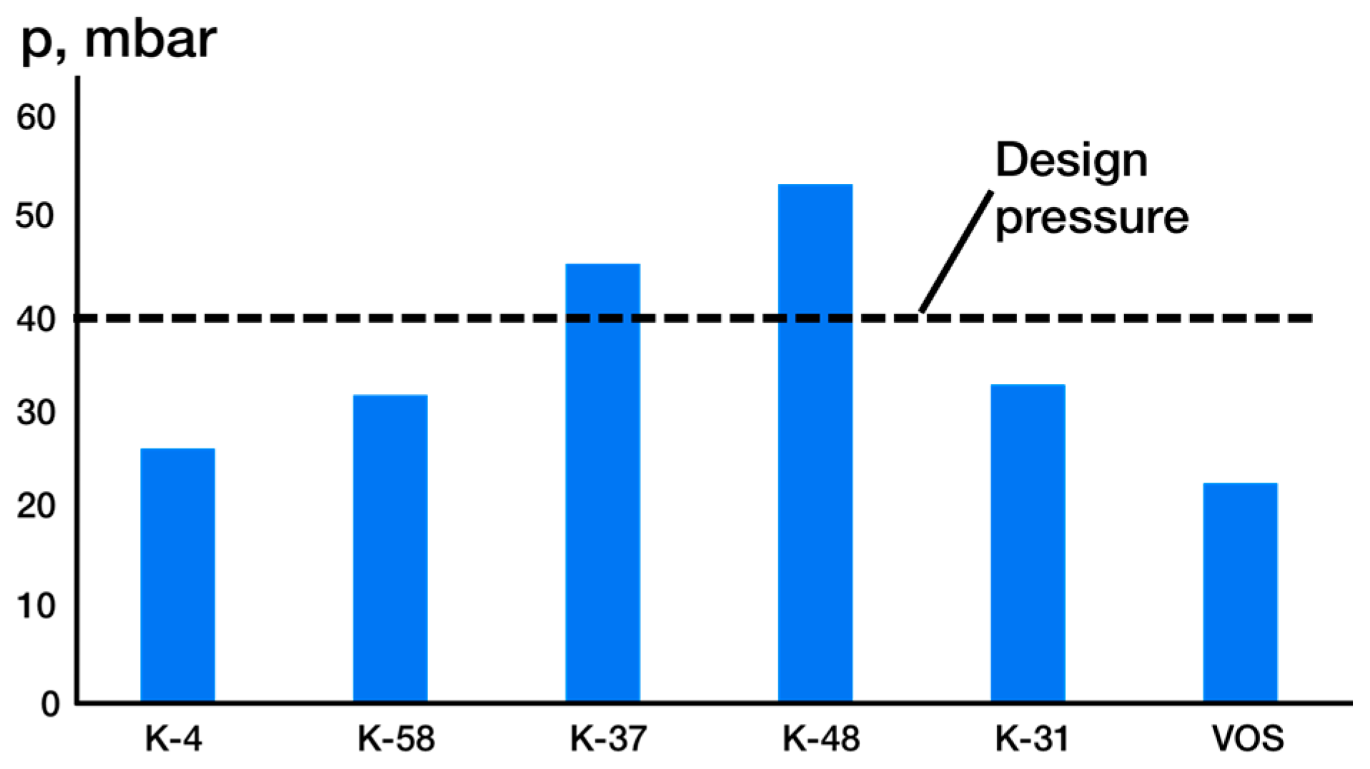
Figure 15 illustrates the pressure distribution of the top of the vacuum columns and the vacuum overhead system (VOS). The results indicate that even though the pressure at the inlet to the liquid-ring vacuum pump (LRVP) is nearly half of the required pressure (40 mm Hg), the pressure at the top of the columns remains close to the design parameter, suggesting that the pipelines exhibit high hydraulic resistances.
The adoption of an increased performance margin has resulted in the successful attainment of the objectives of the reconstruction project, leading to significant cost savings. Notably, had a lower VOS efficiency been chosen, the reconstruction tasks would have been incomplete. Therefore, the decision to raise the performance margin was critical in ensuring the project’s success.
9. Evaluation of the Effectiveness of the Vacuum Overhead System
An efficiency assessment can be made by determining the operating costs for the functioning of the VOS. To do this, according to Formula (15), the costs of the consumed resources are determined:
Further, all costs are summed up and the total operating costs are determined:
Further, according to Formula (17), the economic effect of the reconstruction of the existing VSS is determined.
After that, with the accepted capital expenditures, the payback period of the project can be determined by:
The key outcome of the calculation based on the above-described methodology is the payback period of the project, which serves as a determinant for the viability of a particular VOS layout option. Moreover, this approach is considerably sensitive to the prevailing energy resource prices, which are shaped by the production specifics and location. The studies in [36,37] proposed prices for fundamental energy resources that were employed to estimate the economic impact. Prices for energy resources are provided in Table 8.
It is worth noting that the production of electricity and water vapor is typically achieved through the combustion of various types of fuels. Therefore, an alternative method for assessing energy efficiency in the operation of a vacuum overhead system is to convert the energy consumed into units of conventional fuel, which enables the estimation of pollutant emissions (e.g., CO2). Conventional fuel is a standard unit for accounting for organic fuel in calculations, used to determine the useful effects of various types of fuels in their overall accounting. It is assumed that the combustion of 1 kg of solid (liquid) or 1 cubic meter of gas releases 29,300 kJ (7000 kcal) of energy. Thus, to calculate the amount of conventional fuel consumed in producing G kilograms per hour of water vapor, the following formula can be used:
If the task is to determine how much conventional fuel needs to be spent to produce N kW of electricity, then you can use the following formula:
In order to estimate the cost of conventional fuel for recycled water based on flow rate, temperature, and pressure, Formula (20) can be utilized to calculate the necessary drive power of feed pumps. Then, Formula (19) can be applied to determine the cost of conventional fuel for producing electricity.
With a known consumption of conventional fuel, it is possible to determine the CO2 output:
In order to evaluate the environmental impact of a vacuum overhead system (VOS), it is important to calculate the emissions of carbon dioxide (CO2) that occur during its operation. The coefficient C1, which corresponds to the formation of CO2 per unit of conventional fuel consumption, can be obtained from reference data. It should be noted that the carbon oxidation coefficient is assumed to be 1.
The calculation of CO2 emissions is a crucial factor in determining the environmental sustainability of a particular type of VOS. In addition to CO2 emissions, the operating costs and conventional fuel costs must also be considered. These values are presented in the Table 9.
The implementation of a hydro-circulatory vacuum overhead system (VOS) presents an opportunity to eliminate the need for costly water usage. Furthermore, based on an annual operating time of 8000 h for the system, the associated costs of the proposed VOS are only a quarter of those for the existing vapor steam stripping (VOS) system. In terms of conventional fuel efficiency, the hydro-circulatory VOS would result in a reduction in the costs of conventional fuel and CO2 emissions by more than threefold. In addition, the hydro-circulatory VOS would eliminate the formation of Chemical Contaminated Condensate (CCC), which would positively impact the environmental conditions at the facility and alleviate the burden on the environment.
10. Conclusions
The problems of designing technological systems for creating a vacuum are relevant and are not widely discussed in scientific literature. This is because, in general, researchers solve local problems by designing a specific process at a specific plant. Furthermore, no methodology exists for designing and calculating technological systems for creating a vacuum, depending on the type of process and equipment used.
Due to the uncertainty in assigning technological parameters for the Vacuum Overhead System (VOS) of an industrial chemical-technological process and the difficulty in determining the load, designers tend to overestimate the size of the selected vacuum pump. This leads to increased consumption of valuable energy resources and the generation of chemically contaminated wastewater. The methodology proposed in the article allows for the utilization of process simulation software capabilities. In this approach, the pressure in the system is not pre-determined but selected to harmonize the characteristics of the main elements of the vacuum block. This eliminates the need for introducing large safety factors since the system is calculated as a whole, considering the mutual influence of its components.
The capabilities of process simulation software allow for the rapid and highly accurate multifactor optimization of vacuum systems, enabling the identification of system bottlenecks. However, the proposed design methodology has significant drawbacks, including:
- The initial models of vacuum blocks and the Vacuum Overhead System (VOS) must be accurate and qualitatively describe the behavior of the technological object over a wide range of input data;
- The primary elements of the model must be tuned to ensure the convergence of calculations across a broad range of input parameters;
- Specialized software is required for managing the process simulation software since it involves comparing different data and assigning initial values based on this comparison;
- Challenges in automating the input of pressure (p) and temperature (t) values.
While these drawbacks are significant, they are not critical, and the proposed methodology can still be applied in the design of vacuum blocks for chemical-technological processes.
The process of selecting a vacuum overhead system for the cumulus method of processing phenol–acetone production waste was described in this paper; mathematical models of the process itself (distillation column), condensation units, and VOS were created for this purpose. The dependencies (volume flow and pressure) were utilized to connect these various elements. During the initial design, a vacuum pump (LRVP) with a performance margin of 40% was chosen. Following the reconstruction, it was discovered that the pressure at the inlet to the vacuum-overhead system was nearly twice as low as in the design.
To determine the reasons for this, modified models of the process and the vacuum overhead system were used based on the results of the post-modernization inspection of the installation, and numerical experiments were performed on the coupling of the characteristics of the block and the vacuum-creating system using the provisions in [36,37,38]. It was discovered that using cooled brine in the condensation unit and phenolic solution as the working fluid of the vacuum overhead system allowed for a significant reduction in the load on the vacuum pump while increasing its productivity. At the same time, the pressure in the individual columns is nearly twice that of the pressure at the system’s inlet.
The example under consideration demonstrated that assigning technological parameters in key nodes of the system a priori can result in both a significant decrease in pressure in the block and failure to achieve the required vacuum value, which necessitates additional research.
Author Contributions
Conceptualization E.V.O. and S.I.P.; methodology, E.V.O. and A.S.P.; software, D.B.; validation E.V.O., S.I.P. and D.B.; formal analysis, E.V.O.; investigation, E.V.O. and A.S.P.; resources, S.I.P.; data curation, A.S.P.; writing—original draft preparation, E.V.O.; writing—review and editing, D.B.; visualization, D.B.; supervision, S.I.P. and E.V.O.; project administration, S.I.P.; funding acquisition, S.I.P. All authors have read and agreed to the published version of the manuscript.
Funding
This research was funded by the Ministry of Science and Higher Education of the Russian Federation grant number 075-01261-22-00 «Energy saving processes of liquid mixtures separation for the recovery of industrial solvents» and the APC was funded by the authors.
Data Availability Statement
The data that supports the findings of this study are available within the article.
Conflicts of Interest
The authors declare no conflicts of interest.
Abbreviations
| AMS | alpha-myethyl styrene; |
| DMFC | Dimethylphenylcarbinol |
| ACP | alpha-myethyl styrene |
| C | CO2—formation coefficient; |
| SEP | steam ejector vacuum pump |
| IPB | isopropylbenzene |
| G | mass flow, kg/hr |
| CCTS | complex chemical and technological systems |
| DC | distillation columns |
| CD | contact devices |
| VO | object under vacuum; |
| VC | vacuum condenser; |
| VOS | vacuum overhead systems |
| L | liquid volume flow, m3/hr; |
| LLE | liquid–liquid equilibrium |
| LE | liquid ejectors |
| LRVP | liquid-ring vacuum pumps |
| TP | communication pipelines |
| K-4, K-31, K-37 | distillation columns |
| K | carbon oxidation coefficient; |
| SGM | steam—gas mixture |
| ECP | external control program; |
| VLE | vapor–liquid equilibrium; |
| VLLE | vapor–liquid–liquid equilibrium; |
| A | coefficients of equations describing physicochemical processes; |
| non-temperature dependent energy parameter between components i and j (cal/gmol); | |
| temperature dependent energy parameter between components i and j (cal/gmol-K); | |
| surface heat exchange margin, %; | |
| output variables vector; | |
| y | molar fraction of component i in vapor phase; |
| x | molar fraction of component i in liquid phase; |
| po | pressure of inflated vapors, mbar; |
| p | pressure, mbar |
| vapor pressure of component i, mbar; | |
| pump power, kW; | |
 P·Δp P·Δp | pressure drop, mbar |
| Input variables vector; | |
| mass flow, kg/hr | |
| acceleration due to gravity, m2/s; | |
| T | temperature, K; |
| t | temperature, °C |
| Vi | molar volume of pure liquid component i in m3/kgmol (litres/gmol) |
| V | volume flow rate, m3/hour |
| V1 | volume flow rate at the outlet, m3/hour |
| V2 | volume flow rate at the inlet, m3/hour |
| leak rate, m3·Pa/s; | |
| Greek | |
| Δ | error, % |
| γ | activity coefficient; |
| vector function; | |
| Subscriptions | |
| diffusion; | |
| permeability; | |
| Min | minimum values; |
| max | maximum value; |
| in | air leak |
| fe | fuel equivalent; |
| t | turbine; |
| b | boiler; |
| p | pump; |
| proc | process; |
| surface; | |
| i, j and k | component number |
| 1 | parameters related to the output; |
| 2 | parameters related to the input. |
Appendix A

Table A1.
Calculated values for the flows indicated in Figure 6.
Table A1.
Calculated values for the flows indicated in Figure 6.
| Name | I | 1 | III | ovh | cond-1 |
|---|---|---|---|---|---|
| Vapor fraction | 0.00 | 0.00 | 0.00 | 1.00 | 0.00 |
| Temperature (°C) | 140.00 ** | 130.52 ** | 180.62 | 103.34 | 40.00 ** |
| Pressure (mm Hg) | 760.04 * | 1500.12 * | 116.56 | 23.00 | 22.62 |
| Molar flow (kgmole/h) | 18.16 | 36.27 | 4.54 | 50.00 | 50.00 |
| Mass flow (kg/h) | 2294.00 ** | 4000.05 ** | 949.92 | 5333.53 | 5333.53 |
| Liquid Volume flow (m3/h) | 2.22 | 3.89 | 0.96 | 5.16 | 5.16 |
| Heat flow (KJ/h) | −2,770,225 | −4,952,186.71 | −803,012.11 | −4,554,105.46 | −7,663,623.96 |
| Name | IX-1 | dist | 2 | ovh-1 | Bottom-2 |
| Vapor fraction | 1.00 | 0.00 | 0.00 | 0.99 | 0.00 |
| Temperature (°C) | 40.00 | 40.00 | 35.00 * | 101.19 | 130.39 |
| Pressure (mm Hg) | 22.62 | 22.62 | 27.75 ** | 31.50 | 83.26 |
| Molar flow (kgmole/h) | 0.12 | 49.89 | 12.28 | 26.05 | 36.28 |
| Mass flow (kg/h) | 3.68 | 5329.85 | 1200.00 ** | 2534.40 | 4000.05 |
| Liquid Volume flow (m3/h) | 0.00 | 5.16 | 1.14 | 2.41 | 3.89 |
| Heat flow (KJ/h) | −389.06 | −7,663,234.90 | −1,842,412.81 | −2,260,965.91 | −4,952,067.72 |
| Name | cond-2 | IX-2 | cond-3 | II | reflux |
| Vapor fraction | 0.0 | 1.00 | 0.00 | 0.00 | 0.00 |
| Temperature (°C) | 35.00 ** | 35.00 | 35.00 | 35.00 | 35.00 |
| Pressure (mm Hg) | 27.75 | 27.75 | 27.75 | 27.75 | 27.75 |
| Molar flow (kgmole/h) | 26.05 | 0.16 | 25.89 | 13.60 | 12.28 |
| Mass flow (kg/h) | 2534.40 | 5.13 | 2529.27 | 1329.27 | 1200.00 * |
| Liquid Volume flow (m3/h) | 2.41 | 0.01 | 2.41 | 1.27 | 1.14 |
| Heat flow (KJ/h) | −3,883,588 | −486.80 | −3,883,101.49 | −2,040,783.96 | −1,842,317.52 |
| Name | 3 | X-1 | X-2 | - | - |
| Vapor fraction | 0.00 | 1.00 | 1.00 | - | - |
| Temperature (°C) | 130.52 | 20.00 * | 20.00 * | - | - |
| Pressure (mm Hg) | 1500.12 ** | 760.04 * | 760.04 ** | - | - |
| Molar flow (kgmole/h) | 36.28 | 0.11 | 0.16 | - | - |
| Mass flow (kg/h) | 4000.05 | 3.21 ** | 4.60 ** | - | - |
| Liquid Volume flow (m3/h) | 3.89 | 0.00 | 0.01 | - | - |
| Heat flow (KJ/h) | −4,950,997 | −15.89 | −22.77 | - | - |
Stream name with (*) represents the calculation data. Values marked with ** denote inputs that were not calculated by the software (except for reflux streams, as they are recycled and were calculated using a special module).
Table A2.
Calculated values for the streams indicated in Figure 7.
Table A2.
Calculated values for the streams indicated in Figure 7.
| Name | IX-3 | IV | VI | Reflux-2 | 11-2 |
|---|---|---|---|---|---|
| Vapor fraction | 1.0 | 0.0 | 0.0 | 0.0 | 1.0 |
| Temperature (°C) | 20.00 * | 160.00 * | 55.00 | 55.16 * | 82.71 |
| Pressure (mm Hg) | 760.04 ** | 760.04 ** | 49.50 | 1500 ** | 53.25 |
| Molar flow (kgmole/h) | 0.14 | 11.00 | 2.92 | 43.05 | 46.08 |
| Mass flow (kg/h) | 3.95 ** | 1305.30 ** | 345.90 | 5100.00 ** | 5452.19 |
| Liquid Volume flow (m3/h) | 0.00 | 1.46 | 0.39 | 5.70 | 6.09 |
| Heat flow (KJ/h) | −19.55 | 821,035.87 | 182,340.96 | 2,692,787.32 | 5,085,198.27 |
| Name | 14-2 | IX-4 | Reflux-1 | to cond-1 | 3 |
| Vapor fraction | 0.00 | 1.00 | 0.00 | 1.00 | 0.01 |
| Temperature (°C) | 55 ** | 20 ** | 45.17 * | 69.26 | 45 ** |
| Pressure (mm Hg) | 49.50 | 760.0 * | 1500.12 * | 45.75 | 42.00 |
| Molar flow (kgmole/h) | 46.08 | 7.53E-02 | 28.30 | 30.46 | 30.46 |
| Mass flow (kg/h) | 5452.19 | 2.18 ** | 3400.00 ** | 3647.25 | 3647.25 |
| Liquid Volume flow (m3/h) | 6.09 | 0.00 | 3.93 | 4.21 | 4.21 |
| Heat flow (KJ/h) | 2,874,260.95 | −10.79 | −968,792.90 | 412,735.44 | −1,033,177.47 |
| Name | X-3 | V | 4 | cond-1 | 5 |
| Vapor fraction | 1.00 | 0.00 | 0.00 | 0.00 | 0.00 |
| Temperature (°C) | 45.00 | 45.00 | 45.00 | 45.00 | 45.17 |
| Pressure (mm Hg) | 42.00 | 42.00 | 42.00 | 42.00 | 1500.12 * |
| Molar flow (kgmole/h) | 0.21 | 1.96 | 28.30 | 30.25 | 28.30 |
| Mass flow (kg/h) | 12.35 | 234.90 | 3400.00 * | 3634.90 | 3400.00 |
| Liquid Volume flow (m3/h) | 0.01 | 0.27 | 3.93 | 4.20 | 3.93 |
| Heat flow (KJ/h) | 675.42 | −66,812.24 | −967,040.65 | −1,033,852.89 | −965,994.01 |
| Name | IX-5 | reflux-3 | Bottom prod-1 | X-4 | bottom prod-2 |
| Vapor fraction | 1.00 | 0.00 | 0.00 | 1.00 | 0.00 |
| Temperature (°C) | 20.00 ** | 60.17 ** | 124.85 | 55.00 | 127.32 |
| Pressure (mm Hg) | 760.04 | 1500.12 * | 236.27 | 49.50 | 247.52 |
| Molar flow (kgmole/h) | 0.09 | 33.00 | 8.98 | 0.11 | 6.02 |
| Mass flow (kg/h) | 2.58 ** | 3900.00 ** | 1062.00 | 6.29 | 711.99 |
| Liquid Volume flow (m3/h) | 0.00 | 4.33 | 1.18 | 0.01 | 0.79 |
| Heat flow (KJ/h) | −12.77 | 2,616,102.33 | 751,196.24 | 3458.36 | 526,180.91 |
| Name | cond-2 | 6 | 7 | to cond-3 | VIII |
| Vapor fraction | 0.00 | 0.00 | 0.00 | 1.00 | 0.00 |
| Temperature (°C) | 55.00 | 55.00 | 55.16 | 74.20 | 127.11 |
| Pressure (mm Hg) | 49.50 | 49.50 | 1500.12 * | 35.00 | 228.77 |
| Molar flow (kgmole/h) | 45.97 | 43.05 | 43.05 | 37.90 | 1.21 |
| Mass flow (kg/h) | 5445.90 | 5100.00 ** | 5100.00 | 4471.07 | 143.49 |
| Liquid Volume flow (m3/h) | 6.09 | 5.70 | 5.70 | 4.97 | 0.16 |
| Heat flow (KJ/h) | 2,870,802.59 | 2,688,461.63 | 2,689,971.44 | 4,748,832.61 | 71,468.00 |
| Name | 8 | X-5 | cond-3 | 10 | VII |
| Vapor fraction | 0.01 | 1.00 | 0.00 | 0.00 | 0.00 |
| Temperature (°C) | 60.00 ** | 60.00 | 60.00 | 60.00 | 60.00 |
| Pressure (mm Hg) | 31.25 | 31.25 | 31.25 | 31.25 | 31.25 |
| Molar flow (kgmole/h) | 37.90 | 0.21 | 37.69 | 33.00 | 4.69 |
| Mass flow (kg/h) | 4471.07 | 17.22 | 4453.85 | 3900.00 ** | 553.85 |
| Liquid Volume flow (m3/h) | 4.97 | 0.02 | 4.95 | 4.33 | 0.62 |
| Heat flow (KJ/h) | 3,001,246.98 | 15,374.97 | 2,985,872.01 | 2,614,568.91 | 371,303.10 |
| Name | 11 | - | - | - | - |
| Vapor fraction | 0.00 | - | - | - | - |
| Temperature (°C) | 60.17 | - | - | - | - |
| Pressure (mm Hg) | 1500.12 ** | - | - | - | - |
| Molar flow (kgmole/h) | 33.00 | - | - | - | - |
| Mass flow (kg/h) | 3900.00 | - | - | - | - |
| Liquid Volume flow (m3/h) | 4.33 | - | - | - | - |
| Heat flow (KJ/h) | 2,615,734.78 | - | - | - | - |
Stream name with (*) represents the calculation data. Values marked with ** denote inputs that were not calculated by the software (except for reflux streams, as they are recycled and were calculated using a special module).
Table A3.
Composition of the flows indicated in Figure 6.
Table A3.
Composition of the flows indicated in Figure 6.
| Name | I | 1 | III | ovh | cond-1 |
|---|---|---|---|---|---|
| Mass fraction (Phenol) | 0.488 ** | 0.429 ** | 0.010 | 0.530 | 0.530 |
| Mass fraction (Acetophenone) | 0.084 ** | 0.367 ** | 0.050 | 0.311 | 0.311 |
| Mass fraction (DMPC) | 0.013 ** | 0.186 ** | 0.000 | 0.145 | 0.145 |
| Mass fraction (Cumylphenol) | 0.220 ** | 0.000 ** | 0.400 | 0.000 | 0.000 |
| Mass fraction (Phenol tar) | 0.220 * | 0.017 * | 0.540 | 0.012 | 0.012 |
| Mass fraction (Airl) | 0.000 * | 0.000 * | 0.000 | 0.001 | 0.001 |
| Name | IX-1 | dist | 2 | ovh-1 | Bottom-2 |
| Mass fraction (Phenol) | 0.09 | 0.53 | 0.84 ** | 0.84 | 0.43 |
| Mass fraction (Acetophenone) | 0.04 | 0.31 | 0.14 ** | 0.14 | 0.37 |
| Mass fraction (DMPC) | 0.01 | 0.15 | 0.02 ** | 0.02 | 0.19 |
| Mass fraction (Cumylphenol) | 0.00 | 0.00 | 0.00 ** | 0.00 | 0.00 |
| Mass fraction (Phenol tar) | 0.00 | 0.01 | 0.00 * | 0.00 | 0.02 |
| Mass fraction (Airl) | 0.87 | 0.00 | 0.00 * | 0.00 | 0.00 |
| Name | cond-2 | IX-2 | cond-3 | II | reflux |
| Mass fraction (Phenol) | 0.84 | 0.10 | 0.84 | 0.84 | 0.84 |
| Mass fraction (Acetophenone) | 0.14 | 0.00 | 0.14 | 0.14 | 0.14 |
| Mass fraction (DMPC) | 0.02 | 0.00 | 0.02 | 0.02 | 0.02 |
| Mass fraction (Cumylphenol) | 0.00 | 0.00 | 0.00 | 0.00 | 0.00 |
| Mass fraction (Phenol tar) | 0.00 | 0.00 | 0.00 | 0.00 | 0.00 |
| Mass fraction (Airl) | 0.00 | 0.90 | 0.00 | 0.00 | 0.00 |
| Name | 3 | X-1 | X-2 | - | - |
| Mass fraction (Phenol) | 0.43 | 0.00 ** | 0.00 ** | - | - |
| Mass fraction (Acetophenone) | 0.37 | 0.00 * | 0.00 ** | - | - |
| Mass fraction (DMPC) | 0.19 | 0.00 ** | 0.00 ** | - | - |
| Mass fraction (Cumylphenol) | 0.00 | 0.00 ** | 0.00 ** | - | - |
| Mass fraction (Phenol tar) | 0.02 | 0.00 ** | 0.00 ** | - | - |
| Mass fraction (Airl) | 0.00 | 1.00 ** | 1.00 ** | - | - |
Stream name with (*) represents the calculation data. Values marked with ** denote inputs that were not calculated by the software (except for reflux streams, as they are recycled and were calculated using a special module).
Table A4.
Composition of the flows indicated in Figure 7.
Table A4.
Composition of the flows indicated in Figure 7.
| Name | IX-3 | IV | VI | Reflux-2 | 11-2 |
|---|---|---|---|---|---|
| Mass fraction (IPB) | 0.000 ** | 0.222 ** | 0.144 | 0.143 ** | 0.144 |
| Mass fraction (AMS) | 0.000 ** | 0.759 ** | 0.856 | 0.857 ** | 0.856 |
| Mass fraction (Acetophenone) | 0.000 ** | 0.019 ** | 0.000 | 0.000 ** | 0.000 |
| Mass fraction (Air) | 1.000 ** | 0.000 ** | 0.000 | 0.000 * | 0.000 |
| Name | 14-2 | IX-4 | Reflux-1 | to cond-1 | 3 |
| Mass fraction (IPB) | 0.144 | 0.000 ** | 0.980 * | 0.978 | 0.978 |
| Mass fraction (AMS) | 0.856 | 0.000 ** | 0.020 * | 0.021 | 0.021 |
| Mass fraction (Acetophenone) | 0.000 | 0.000 ** | 0.000 * | 0.000 | 0.000 |
| Mass fraction (Air) | 0.000 | 1.000 ** | 0.000 * | 0.001 | 0.001 |
| Name | X-3 | V | 4 | cond-1 | 5 |
| Mass fraction (IPB) | 0.672 | 0.979 | 0.979 | 0.979 | 0.979 |
| Mass fraction (AMS) | 0.008 | 0.021 | 0.021 | 0.021 | 0.021 |
| Mass fraction (Acetophenone) | 0.000 | 0.000 | 0.000 | 0.000 | 0.000 |
| Mass fraction (Air) | 0.320 | 0.000 | 0.000 | 0.000 | 0.000 |
| Name | IX-5 | reflux-3 | Bottom prod-1 | X-4 | bottom prod-2 |
| Mass fraction (IPB) | 0.000 ** | 0.001 ** | 0.051 | 0.144 | 0.001 |
| Mass fraction (AMS) | 0.000 ** | 0.998 ** | 0.926 | 0.509 | 0.964 |
| Mass fraction (Acetophenone) | 0.000 ** | 0.001 ** | 0.024 | 0.000 | 0.035 |
| Mass fraction (Air) | 1.000 ** | 0.000 ** | 0.000 | 0.347 | 0.000 |
| Name | cond-2 | 6 | 7 | to cond-3 | VIII |
| Mass fraction (IPB) | 0.144 | 0.144 | 0.144 | 0.001 | 0.000 |
| Mass fraction (AMS) | 0.856 | 0.856 | 0.856 | 0.998 | 0.831 |
| Mass fraction (Acetophenone) | 0.000 | 0.000 | 0.000 | 0.001 | 0.169 |
| Mass fraction (Air) | 0.000 | 0.000 | 0.000 | 0.001 | 0.000 |
| Name | 8 | X-5 | cond-3 | 10 | VII |
| Mass fraction (IPB) | 0.001 | 0.001 | 0.001 | 0.001 | 0.001 |
| Mass fraction (AMS) | 0.998 | 0.849 | 0.998 | 0.998 | 0.998 |
| Mass fraction (Acetophenone) | 0.001 | 0.000 | 0.001 | 0.001 | 0.001 |
| Mass fraction (Air) | 0.001 | 0.150 | 0.000 | 0.000 | 0.000 |
| Name | 11 | - | - | - | - |
| Mass fraction (IPB) | 0.001 | - | - | - | - |
| Mass fraction (AMS) | 0.998 | - | - | - | - |
| Mass fraction (Acetophenone) | 0.001 | - | - | - | - |
| Mass fraction (Air) | 0.000 | - | - | - | - |
Stream name with (*) represents the calculation data. Values marked with ** denote inputs that were not calculated by the software (except for reflux streams, as they are recycled and were calculated using a special module).
References
- Hoffman, D.M. Handbook of Vacuum Science and Technology; Academic Press: Cambridge, MA, USA, 1997. [Google Scholar]
- Umrath, W. Fundamentals of Vacuum Technology; Oerlikon Leybold Vacuum Gmbh: Cologne, Germany, 2007. [Google Scholar]
- Martin, L.H.; Hill, R.D. A Manual of Vacuum Practice; University of Melbourne Press: Melbourne, Australia, 1947. [Google Scholar]
- Danilin, V.S. Vacuum Pumps and Systems; Tocenergoisdat: Moscow, Russia, 1957. [Google Scholar]
- Martin, G.R.; Lines, J.R.; Golden, S.W. Understanding Vacuum-System Fundamentals. Hydrocarbon Processing 1994. pp. 1–7. Available online: https://graham-mfg.com/wp-content/uploads/2023/02/Understand-Vacuum-System-Fundamentals.pdf (accessed on 22 February 2024).
- Gaikwad, W.; Warade, A.R.; Bhagat, S.L.; Bhasarkar, J.B. Optimization and Simulation of Refinery Vacuum Column with an Overhead Condenser. Mater. Today Proc. 2022, 57, 1593–1597. [Google Scholar] [CrossRef]
- Rom, A.; Miltner, A.; Wukovits, W.; Friedl, A. Energy Saving Potential of Hybrid Membrane and Distillation Process in Butanol Purification: Experiments, Modelling and Simulation. Chem. Eng. Process. Process Intensif. 2016, 104, 201–211. [Google Scholar] [CrossRef]
- Kancherla, R.; Nazia, S.; Kalyani, S.; Sridhar, S. Modeling and Simulation for Design and Analysis of Membrane-Based Separation Processes. Comput. Chem. Eng. 2021, 148, 107258. [Google Scholar] [CrossRef]
- Li, X.; Cui, C.; Sun, J. Enhanced Product Quality in Lubricant Type Vacuum Distillation Unit by Implementing Dividing Wall Column. Chem. Eng. Process.—Process Intensif. 2018, 123, 1–11. [Google Scholar] [CrossRef]
- Habibullah, A. Crude and Vacuum Unit Design Challenges. J. Chem. Eng. 2017. Available online: https://www.researchgate.net/publication/318405793_CRUDE_AND_VACUUM_UNIT_DESIGN_CHALLENGES (accessed on 22 February 2024).
- Sohrabali, G.; Shahryar, J.N. Ejector Modeling and Examining the Possibility of Replacing Liquid Vacuum Pump in Vacuum Production Systems. Int. J. Chem. Eng. Appl. 2011, 2, 91–97. [Google Scholar]
- Coker, A.K. Ludwig’s Applied Process Design for Chemical and Petrochemical Plants; Elsevier Inc.: Amsterdam, The Netherlands, 2007. [Google Scholar]
- Hicks, T.G. Handbook of Mechanical Engineering Calculations; McGRAW-HILL Professional: New York, NY, USA, 2006. [Google Scholar]
- Standards of the Tubular Exchanger Manufacturers Association, 10th ed.; TEMA, Inc.: Tarrytown, NY, USA, 2019; Section 5:1.1.1.
- Leybold GmbH. Vacuum Calculations. Available online: https://calc.leybold.com/en/ (accessed on 22 February 2024).
- VacTran. Vacuum Technology Software. Available online: https://www.lesker.com/newweb/technical_info/vactran.cfm (accessed on 22 February 2024).
- Unisim Design. In Tutorials and Applications; Honeywell: Mississauga, ON, Canada, 2017.
- August, D.; Chang, J.; Girbal, S.; Gracia-Perez, D.; Mouchard, G.; Penry, D.A.; Temam, O.; Vachharajani, N. UNISIM: An Open Simulation Environment and Library for Complex Architecture Design and Collaborative Development. IEEE Comput. Arch. Lett. 2007, 6, 45–48. [Google Scholar] [CrossRef]
- Bartolome, P.S.; Van Gerven, T. A comparative study on Aspen Hysys interconnection methodologies. Comput. Chem. Eng. 2022, 162, 107785. [Google Scholar] [CrossRef]
- Miranda, T.d.C.R.D.d.; Figueiredo, F.R.; de Souza, T.A.; Ahón, V.R.R.; Prata, D.M. Eco-efficiency analysis and intensification of cryogenic extractive distillation process for separating CO2–C2H6 azeotrope through vapor recompression strategy. Chem. Eng. Process.—Process Intensif. 2024, 196, 109636. [Google Scholar] [CrossRef]
- Paiva, M.; Vieira, A.; Gomes, H.T.; Brito, P. Simulation of a Downdraft Gasifier for Production of Syngas from Different Biomass Feedstocks. ChemEngineering 2021, 5, 20. [Google Scholar] [CrossRef]
- Vaccari, M.; Pannocchia, G.; Tognotti, L.; Paci, M. Rigorous simulation of geothermal power plants to evaluate environmental performance of alternative configurations. Renew. Energy 2023, 207, 471–483. [Google Scholar] [CrossRef]
- Baynazarov, I.Z.; Lavrenteva, Y.S.; Akhmetov, I.V.; Gubaydullin, I.M. Mathematical Model of the Process of Production of Phenol and Acetone from Cumene Hydroperoxide. J. Phys. Conf. Ser. 2018, 1096, 012197. [Google Scholar] [CrossRef]
- Osipov, E.V.; Ponikarov, S.I.; Telyakov, E.S.; Sadykov, K.S. Reconstruction of Vacuum Overhead Systems of the Department of Waste Processing of Phenol-Acetone Production. Bull. Kazan Technol. Univ. 2011, 18, 193–201. [Google Scholar]
- Powers, R.B. Steam Jet Ejectors for the Process Industries; McGraw-Hill: New York, NY, USA, 1994. [Google Scholar]
- Edwards, J.E. Chemical Engineering in Practice: Design, Simulation and Implementation; P & I Design Ltd.: Stockton-on-Tees, UK, 2011. [Google Scholar]
- Wilson, G.M. Vapor-Liquid Equilibrium. XI. A New Expression for the Excess Free Energy of Mixing. J. Am. Chem. Soc. 1964, 86, 127. [Google Scholar] [CrossRef]
- Renon, H.; Prausnitz, J.M. Local Compositions in Thermodynamic Excess Functions for Liquid Mixtures. AIChE J. 1968, 14, 135–144. [Google Scholar] [CrossRef]
- Abrams, D.S.; Prausnitz, J.M. Statistical Thermodynamics of liquid mixtures: A new expression for the Excess Gibbs Energy of Partly or Completely Miscible Systems. AIChE J. 1975, 21, 116–128. [Google Scholar] [CrossRef]
- Dyckman, A.S.; Boyarsky, V.P.; Malinovskii, A.S.; Petrov, Y.I.; Krasnov, L.M.; Zinenkov, A.V.; Gorovits, B.I.; Chernukhim, S.N.; Sorokin, A.D.; Fulmer, J.W. Phenol Tar Processing Method. U.S. Patent 5,672,774A, 30 September 1997. [Google Scholar]
- Reddy, C.C.S.; Rangaiah, G.P. Retrofit of Vacuum Systems in Process Industries. In Chemical Process Retrofitting and Revamping: Techniques and Applications; John Wiley & Sons, Ltd.: Hoboken, NJ, USA, 2016; pp. 317–346. [Google Scholar] [CrossRef]
- Govoni, P. An Overview of Vacuum System Design. Chem. Eng. 2017, 124, 52–60. [Google Scholar]
- Golden, S.; Barletta, T.; White, S. Vacuum unit performance. GEA Wiegand. Petrol. Technol. Q. 2012, 17, 131. [Google Scholar]
- Sterling Fluid Systems Group. Liquid Ring Vacuum Pumps & Compressors: Technical Details & Fields of Application. 2017. Available online: https://www.scribd.com/document/487161329/ZHidkostno-Koltsevyie-Nasosyi-i-Kompressoryi-Harakteristiki-i-Primenenie-Liquid-Ring-Vacuum-Pumps-Compressors-Technical-Details-Fields-of-Applicatio (accessed on 22 February 2024).
- Aliasso, J. How to Make Sure You Select the Right Dry Vacuum Pump. World Pumps 2000, 2000, 26–27. [Google Scholar] [CrossRef]
- Osipov, E.V.; Telyakov, E.S.; Ponikarov, S.; Bugembe, D.; Ponikarov, A. Mini-Refinery Vacuum Unit: Functional Analysis and Improvement of Vacuum Overhead System. Processes 2021, 9, 1865. [Google Scholar] [CrossRef]
- Osipov, E.V.; Telyakov, E.S.; Ponikarov, S.I. Coupled Simulation of a Vacuum Creation System and a Rectification Column Block. Processes 2020, 8, 1333. [Google Scholar] [CrossRef]
- Osipov, É.V.; Telyakov, É.S.; Latyipov, R.M.; Bugembe, D. Influence of Heat and Mass Exchange in a Liquid Ring Vacuum Pump on Its Working Characteristics. J. Eng. Phys. Thermophys. 2019, 92, 1055–1063. [Google Scholar] [CrossRef]
- Karmanov, E.; Lebedev, Y.; Chekmenev, V.; Aleksandrov, I. Ejector Systems. Chem. Technol. Fuels Oils 2004, 40, 80–83. [Google Scholar] [CrossRef]
- Giproneftemash, M. (Ed.) Steam Jet Vacuum Pumps; Schutte & Koerting: Moscow, Russia, 1965. [Google Scholar]
- Zou, Y.; Jiang, H.; Liu, Y.; Gao, H.; Xing, W.; Chen, R. Highly Efficient Synthesis of Cumene via Benzene Isopropylation over Nano-sized Beta Zeolite in a Submerged Ceramic Membrane Reactor. Sep. Purif. Technol. 2016, 170, 49–56. [Google Scholar] [CrossRef]
- Schmidt, R.J. Industrial Catalytic Processes—Phenol Production. Appl. Catal. A Gen. 2005, 280, 89–103. [Google Scholar] [CrossRef]
- Verma, R.K. IHS Markit|PEP Review 2020-02 Phenol Production by ExxonMobil 3-Step Process. 2020. Available online: https://cdn.ihsmarkit.com/www/pdf/0420/RW2020-02_toc.pdf (accessed on 22 February 2024).
- Zou, B.; Hu, Y.; Huang, X.; Zhou, X.; Huang, H. Manufacturing and New Technology Research of Phenol. Shiyou Huagong/Petrochem. Technol. 2009, 38, 575–580. [Google Scholar]
- Zakoshansky, V.M. Alternative Technologies for Obtaining Phenol. Russ. Chem. J. 2008, 52, 53–71. [Google Scholar]
- Zakoshansky, V.M. Mechanism and Kinetics of Acid-Catalyzed Decomposition of Cumene Hydroperoxide. Catal. Chem. Petrochem. Ind. 2004, 4, 3–15. [Google Scholar]
- Kruzhalov, B.D.; Golovanenko, B.N. Joint Production of Phenol and Acetone; Goskhimizdat, M., Ed.; Goskhimizdat: Moscow, Russia, 1963; 191p. [Google Scholar]
- Zakoshansky, V. Actual Performance of Key Stages of the Phenol Process: Present State and Expected Future. Russ. J. Appl. Chem. 2013, 86, 1118–1140. [Google Scholar] [CrossRef]
- Perego, C.; Ingallina, P. Recent Advances in the Industrial Alkylation of Aromatics: New Catalysts and New Processes. Catal. Today 2002, 73, 3–22. [Google Scholar] [CrossRef]
Figure 1.
Decomposition of a typical chemical-technological process conducted under vacuum.

Figure 4.
Flowchart of the coupled modeling methodology for vacuum blocks.

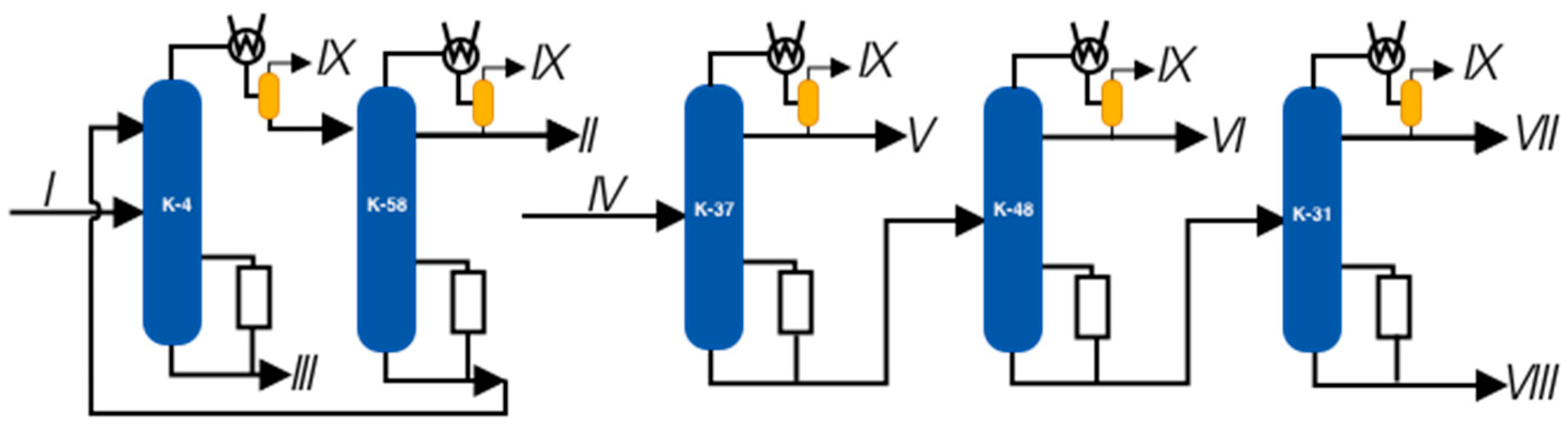
Figure 5.
Vacuum columns of a plant for processing phenol and acetone production waste. I—K-4 column feed; II—phenolic fraction; III—phenolic tar; IV—supply of K-37; V—fraction of isopropylbenzene; VI, VII—fractions of alphamethyl styrene; VIII—residue, IX—flow on the VOS.
Figure 5.
Vacuum columns of a plant for processing phenol and acetone production waste. I—K-4 column feed; II—phenolic fraction; III—phenolic tar; IV—supply of K-37; V—fraction of isopropylbenzene; VI, VII—fractions of alphamethyl styrene; VIII—residue, IX—flow on the VOS.

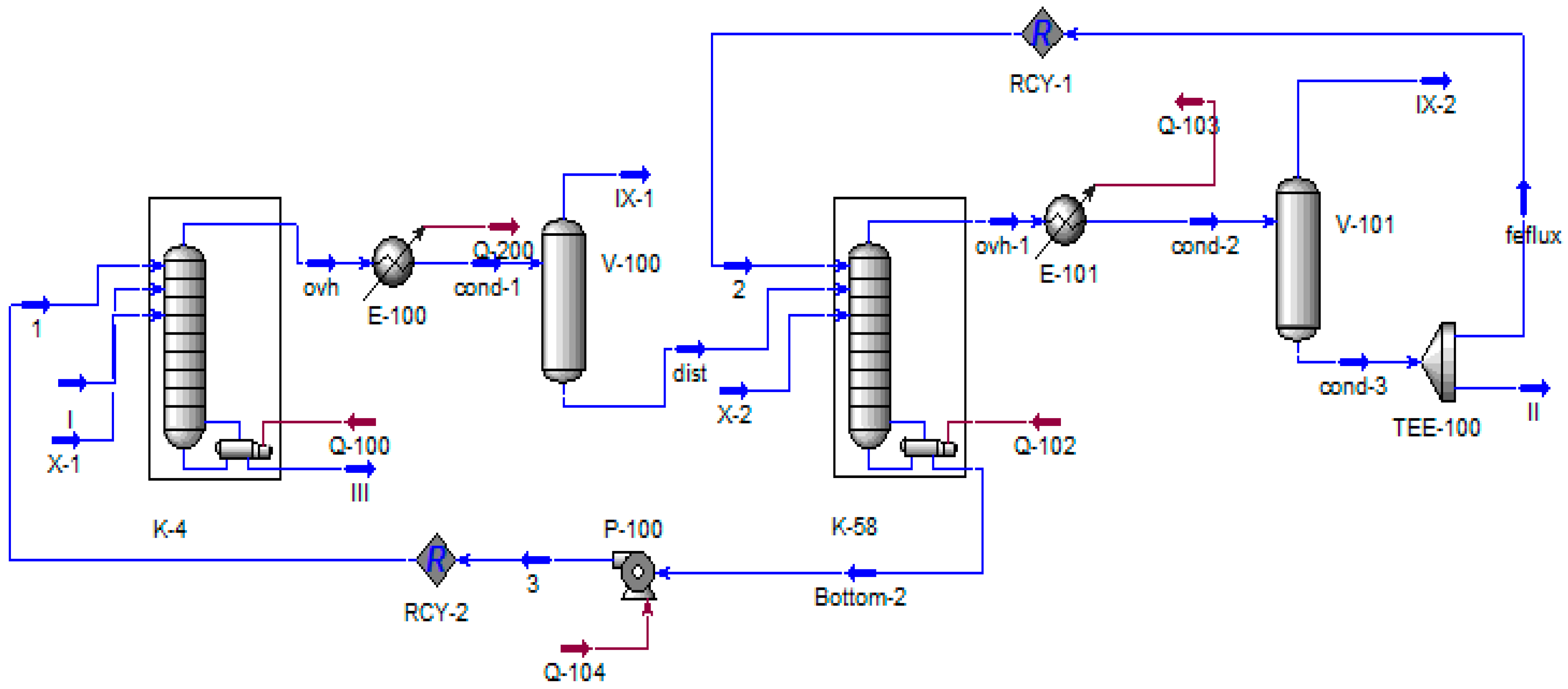
Figure 6.
Process flow diagram of columns K-4 and K-58. I—K-4 column feed; II—phenolic fraction; III—phenolic tar; IX—flow on the VOS; X—air leak rate.
Figure 6.
Process flow diagram of columns K-4 and K-58. I—K-4 column feed; II—phenolic fraction; III—phenolic tar; IX—flow on the VOS; X—air leak rate.

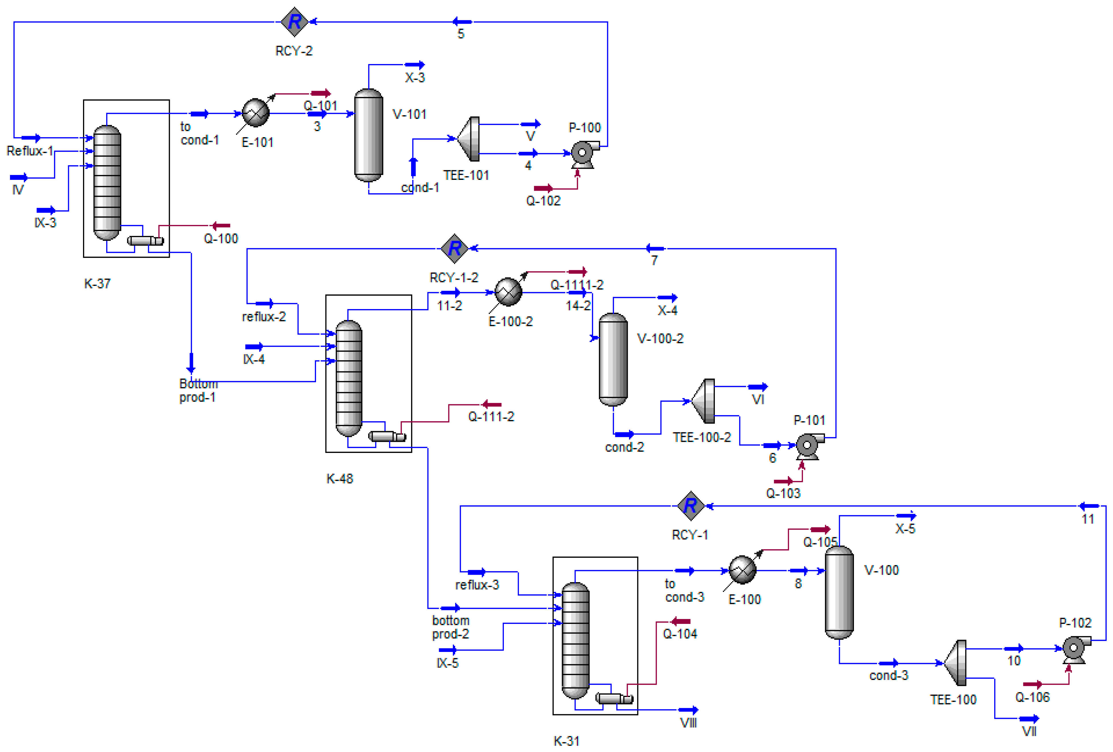
Figure 7.
Process flow diagram of columns K-37, K-48, and K-58. IV—supply of K-37; V—fraction of isopropylbenzene; VI, VII—fractions of alphamethyl styrene; VIII—residue, IX—air leak rate; X—flow on the VOS.
Figure 7.
Process flow diagram of columns K-37, K-48, and K-58. IV—supply of K-37; V—fraction of isopropylbenzene; VI, VII—fractions of alphamethyl styrene; VIII—residue, IX—air leak rate; X—flow on the VOS.

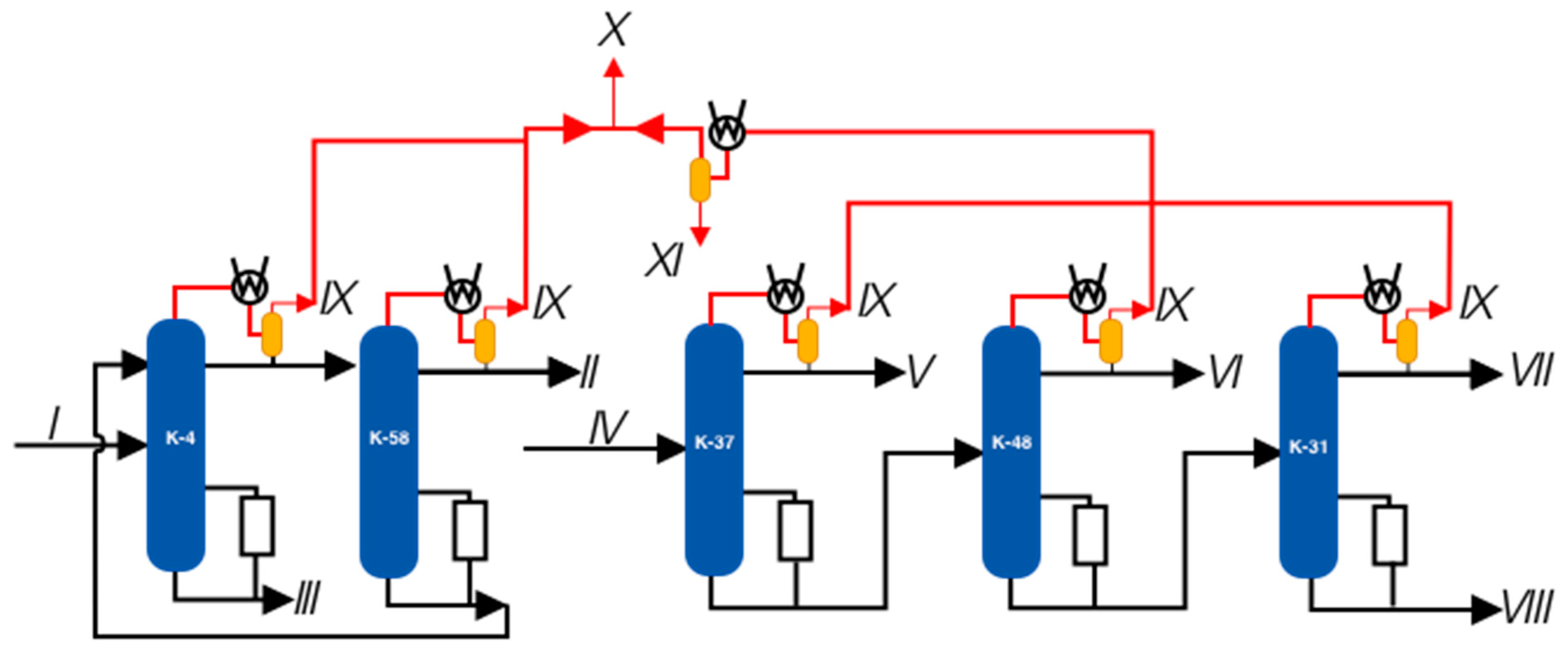
Figure 8.
Block diagram of the proposed reconstruction. I—K-4 column feed; II—phenolic fraction; III—phenolic tar; IV—supply of K-37; V—fraction of isopropylbenzene; VI, VII—fractions of alphamethyl styrene; VIII—residue, IX—flow on the VOS; X—summary flow to VOS; XI—condensate.
Figure 8.
Block diagram of the proposed reconstruction. I—K-4 column feed; II—phenolic fraction; III—phenolic tar; IV—supply of K-37; V—fraction of isopropylbenzene; VI, VII—fractions of alphamethyl styrene; VIII—residue, IX—flow on the VOS; X—summary flow to VOS; XI—condensate.

Figure 9.
Coupling of the characteristics of the pipeline path of the evacuated object and the housing pump.
Figure 9.
Coupling of the characteristics of the pipeline path of the evacuated object and the housing pump.

Figure 10.
Modified process flow diagram of columns K-37, 48, and 31 in Unisim Design R45. IV—supply of K-37; V—fraction of isopropylbenzene; VI, VII—fractions of alphamethyl styrene; VIII—residue, IX—air leak rate; X—flow on the VOS.
Figure 10.
Modified process flow diagram of columns K-37, 48, and 31 in Unisim Design R45. IV—supply of K-37; V—fraction of isopropylbenzene; VI, VII—fractions of alphamethyl styrene; VIII—residue, IX—air leak rate; X—flow on the VOS.

Figure 11.
Modified process flow diagram of columns K-4 and K-58 in Unisim Design R45. I—K-4 column feed; II—phenolic fraction; III—phenolic tar; IX—air leak rate; X—flow on the VOS.
Figure 11.
Modified process flow diagram of columns K-4 and K-58 in Unisim Design R45. I—K-4 column feed; II—phenolic fraction; III—phenolic tar; IX—air leak rate; X—flow on the VOS.

Figure 12.
Process flow diagram for calculating the load on the VOS in Unisim Design R45.

Figure 13.
Simulation flowchart. VO and VOS.

Figure 14.
Coupling of the characteristics of the vacuum column block and the VOS.

Figure 15.
Pressure distribution across columns and VOS.

Table 1.
Survey results.
| Column № | Pressure in the Helmet Line, mmHg. | Condensation Temperature, °C |
|---|---|---|
| 4 | 14 | 40 |
| 58 | 22 | 35 |
| 37 | 65 | 45 |
| 48 | 100 | 55 |
| 31 | Over 100 | 70 |
Table 2.
Parameters of components in the Wilson equation.
| IPB | AMS | Acetophenone | Air | Phenol | Cumylphenol | DMPC | Phenol Tar | |
|---|---|---|---|---|---|---|---|---|
| IPB | - | 57.60 | 335.69 | 829.40 | 1324.01 | 869.43 | 1013.17 | 18.02 |
| AMS | −51.14 | - | 273.39 | 1008.22 | 761.73 | 599.15 | 749.16 | 101.65 |
| Acetophenone | 112.84 | 60.59 | - | - | 3175.79 | −4.76 | 120.53 | - |
| Air | 1445.89 | 2145.26 | - | - | - | - | - | - |
| Phenol | −27.95 | 25.48 | −1335.68 | - | - | −929.53 | −776.69 | - |
| Cumylphenol | 76.48 | 68.27 | 121.00 | 3172.93 | 1499.71 | 646.19 | 814.84 | 270.26 |
| DMPC | −2.67 | 88.21 | 211.48 | - | −388.44 | −250.98 | - | - |
| Phenol tar | 61.17 | 101.47 | - | - | - | - | - | - |
Table 3.
Technological parameters of the column and calculation data for columns K-3 and K-58.
| Stream Name | Composition, Mass Fraction. | Temperature, °C | Flow Rate, kg/hr | ||||
|---|---|---|---|---|---|---|---|
| Phenol | Acetophenone | DMPC | Cumylphenol | Phenol Tar | |||
| I | 0.48 | 0.08 | 0.012 | 0.2 | 0.22 | <150 | 2294 |
| I * | 0.48 | 0.08 | 0.012 | 0.2 | 0.22 | 140 | 2294 |
| Δ, % | 0 | 0 | 0 | 0 | 0 | 6 | 0 |
| II | 0.97 | 0.02 | 0.01 | - | - | 30–40 | 1362 |
| II * | 0.84 | 0.14 | 0.02 | 0.01 | - | 35 | 1354 |
| Δ, % | 14% | 86% | 47% | 100% | - | 0% | 1% |
| III | 0.08 | 0.13 | 0.03 | 0.36 | 0.4 | 122 | 932 |
| III * | 0.01 | 0.05 | - | 0.4 | 0.54 | 180 | 940 |
| Δ, % | 88% | 62% | - | 11% | 26% | 48% | 1% |
Stream name with (*) represents the calculation data.
Table 4.
Technological parameters of the column and calculation data for columns K-37, 48, and 31.
| Stream Name | Composition, Mass Fraction. | Temperature, °C | Flow Rate, kg/hr | ||
|---|---|---|---|---|---|
| IPB | AMS | Acetophenone | |||
| IV | 0.22 | 0.76 | 0.02 | <170 | 1305.3 |
| IV * | 0.221 | 0.76 | 0.019 | 170 | 1305 |
| Δ, % | 0.5% | 0.0% | 5.3% | 0.0% | 0.0% |
| V | 0.98 | 0.015 | 0.05 | 30–40 | 242.5 |
| V * | 0.98 | 0.02 | - | 40 | 239.5 |
| Δ, % | 0% | 25% | - | 0% | 1% |
| VI | 0.081 | 0.92 | 0.001 | 30–40 | 350 |
| VI * | 0.14 | 0.85 | 0.01 | 40 | 349 |
| Δ, % | 42.1% | 8.2% | 90.0% | 0.0% | 0.3% |
| VII | 0.02 | 0.96 | 0.02 | 30–40 | 568 |
| VII * | 0.01 | 0.98 | 0.01 | 40 | 563 |
| Δ, % | 50.0% | 2.1% | 50.0% | 0.0% | 0.9% |
| VIII | - | 0.84 | 0.16 | 122 | 143.5 |
| VIII * | - | 0.83 | 0.17 | 127 | 143.5 |
| Δ, % | - | 1.2% | 5.9% | 3.9% | 0.0% |
Stream name with (*) represents the calculation data.
Table 5.
Parameters of the pumped mixture.
| Parameter | Value |
|---|---|
| Pressure, mm Hg | 40 |
| Temperature, °C | 35 |
| Consumption, kg/hour | 25 |
| Composition, (mass fraction) | |
| IPB | 0.16 |
| AMS | 0.04 |
| Acetophenone | 0.006 |
| Air | 0.794 |
| Phenol | - |
| Cumylphenol | - |
| DMPC | - |
Table 6.
Ranges of values.
| Parameters | Value | Unit of Measurement |
|---|---|---|
| p1 | 15 | mbar |
| p2 | 60 | mbar |
| t1 | 20 | °C |
| t2 | 40 | °C |
| e | 5 | % |
| V2 | 1.1∙V1 | - |
| Δp | 0.4∙p | - |
Table 7.
Comparison of technological parameters of columns with calculation results.
| Parameter | Survey Data | Calculation Data | Unit of Measurement | Δ, % |
|---|---|---|---|---|
| K-4 | ||||
| Top pressure | 23 | 26 | mm Hg | 13% |
| Top temperature K-4 | 93 | 103 | °C | 11% |
| Bottom temperature | 122 | 180 | °C | 48% |
| K-58 | ||||
| Top pressure | 31.5 | 32 | mm Hg | 2% |
| Top temperature | 106.8 | 101.2 | °C | 5% |
| Bottom temperature | 123.9 | 130 | °C | 5% |
| Reflux rate | 1203 | 1200 | kg/hr | 0% |
| K-37 | ||||
| Top pressure | 45.75 | 45 | mm Hg | 2% |
| Top temperature | 63.3 | 69.26 | °C | 9% |
| Bottom temperature | 111 | 124 | °C | 12% |
| Reflux rate | 3400 | 3400 | kg/hr | 0% |
| K-48 | ||||
| Top pressure | 58.5 | 53.25 | mm Hg | 9% |
| Top temperature | 78.7 | 87.1 | °C | 11% |
| Bottom temperature | 111 | 124 | °C | 12% |
| Reflux rate | 4900 | 5100 | kg/hr | 4% |
| K-31 | ||||
| Top pressure | 30.25 | 33 | mm Hg | 9% |
| Top temperature | 78.5 | 74.2 | °C | 5% |
| Bottom temperature | 131.5 | 127.1 | °C | 3% |
| Reflux rate | 4000 | 3900 | kg/hr | 3% |
| VOS | ||||
| Suction pressure | - | 22.5 | mm Hg | - |
| Temperature of the service liquid at the inlet | 5 | 5.5 | °C | 10% |
| The temperature of the service fluid at the outlet | 11.8 | 11.6 | °C | 2% |
Table 8.
Energy prices.
| Resource Name | Value | Unit of Measurement |
|---|---|---|
| Water vapor | 15.28 | USD/Gcal |
| Recycled water | 0.021 | USD/m3 |
| Electricity | 0.04 | USD/kW |
| Cleaning the Chemical Contaminated Condensate | 0.16 | USD/m3 |
The above prices were converted using RUB/USD exchange rate of 28 August 2023.
Table 9.
Comparison of the current and reconstructed VOS.
| № | Parameter | Unit | Type of VOS | |
|---|---|---|---|---|
| Current | LRVP | |||
| 1 | Steam consumption | kg/hr | 300 | 0 |
| 2 | Steam consumption | Gcal/hr | 0.192 | 0 |
| 3 | Recycled water | m3/hr | 10 | 2 |
| 4 | consumption Electricity consumption | kW | 1.09 | 18 |
| 5 | Conditional fuel consumption | t/hr | 33.196 | 6.914095 |
| 6 | CO2 emissions | kg/hr | 0.033 | 0.008988 |
| 7 | Resource prices | |||
| 8 | Water vapor | USD/Gcal | 14.079 | |
| 9 | Recycled water | USD/m3 | 0.020 | |
| Cleaning of Chemical Contaminated Condensate | USD/m4 | 0.153 | ||
| 10 | Electricity | USD/kW | 0.039 | |
| 11 | Costs (8000 h per year) | |||
| 12 | Water vapor | USD/fe | 21,682.71 | 0 |
| 13 | Recycled water | USD/fe | 1578.94 | 315.79 |
| 14 | Electricity | USD/fe | 344.21 | 5684.21 |
| Cleaning of Chemical Contaminated Condensate | USD/fe | 366.31 | 0 | |
| 15 | Total | USD/fe | 23,972.18 | 6000 |
| 16 | % of the baseline | % | 100% | 25% |
Disclaimer/Publisher’s Note: The statements, opinions and data contained in all publications are solely those of the individual author(s) and contributor(s) and not of MDPI and/or the editor(s). MDPI and/or the editor(s) disclaim responsibility for any injury to people or property resulting from any ideas, methods, instructions or products referred to in the content. |
© 2024 by the authors. Licensee MDPI, Basel, Switzerland. This article is an open access article distributed under the terms and conditions of the Creative Commons Attribution (CC BY) license (https://creativecommons.org/licenses/by/4.0/).
Share and Cite
MDPI and ACS Style
Osipov, E.V.; Bugembe, D.; Ponikarov, S.I.; Ponikarov, A.S. Comprehensive Modeling of Vacuum Systems Using Process Simulation Software. ChemEngineering 2024, 8, 31. https://0-doi-org.brum.beds.ac.uk/10.3390/chemengineering8020031
AMA Style
Osipov EV, Bugembe D, Ponikarov SI, Ponikarov AS. Comprehensive Modeling of Vacuum Systems Using Process Simulation Software. ChemEngineering. 2024; 8(2):31. https://0-doi-org.brum.beds.ac.uk/10.3390/chemengineering8020031
Chicago/Turabian StyleOsipov, Eduard Vladislavovich, Daniel Bugembe, Sergey Ivanovich Ponikarov, and Artem Sergeevich Ponikarov. 2024. "Comprehensive Modeling of Vacuum Systems Using Process Simulation Software" ChemEngineering 8, no. 2: 31. https://0-doi-org.brum.beds.ac.uk/10.3390/chemengineering8020031