
Calibrating Agro-Hydrological Model under Grazing Activities and Its Challenges and Implications


1
Sustainable Water Management Research Unit, United States Department of Agricultural Research Service (USDA-ARS), Leland, MS 38756, USA
2
Oklahoma and Central Plains Agricultural Research Center, United States Department of Agricultural Research Service (USDA-ARS), El Reno, OK 73036, USA
*
Author to whom correspondence should be addressed.
Hydrology 2024, 11(4), 42; https://0-doi-org.brum.beds.ac.uk/10.3390/hydrology11040042
Submission received: 23 February 2024
/
Revised: 13 March 2024
/
Accepted: 18 March 2024
/
Published: 22 March 2024
(This article belongs to the Special Issue Hydrological Processes in Agricultural Watersheds)
Abstract
:Recently, the Agricultural Policy Extender (APEX) model was enhanced with a grazing module, and the modified grazing database, APEXgraze, recommends sustainable livestock farming practices. This study developed a combinatorial deterministic approach to calibrate runoff-related parameters, assuming a normal probability distribution for each parameter. Using the calibrated APEXgraze model, the impact of grazing operations on native prairie and cropland planted with winter wheat and oats in central Oklahoma was assessed. The existing performance criteria produced four solutions with very close values for calibrating runoff at the farm outlet, exhibiting equifinality. The calibrated results showed that runoff representations had coefficients of determination and Nash–Sutcliffe efficiencies >0.6 in both watersheds, irrespective of grazing operations. Because of non-unique solutions, the key parameter settings revealed different metrics yielding different response variables. Based on the least objective function value, the behavior of watersheds under different management and grazing intensities was compared. Model simulations indicated significantly reduced water yield, deep percolation, sediment yield, phosphorus and nitrogen loadings, and plant temperature stress after imposing grazing, particularly in native prairies, as compared to croplands. Differences in response variables were attributed to the intensity of tillage and grazing activities. As expected, grazing reduced forage yields in native prairies and increased crop grain yields in cropland. The use of a combinatorial deterministic approach to calibrating parameters offers several new research benefits when developing farm management models and quantifying sensitive parameters and uncertainties that recommend optimal farm management strategies under different climate and management conditions.
1. Introduction
Grazing and haying are options for managing agricultural lands that can provide conservation benefits [1]. To achieve sustainable conservation benefits from grazing operations, it is crucial to understand the relationships among erosion, vegetation, and grazing. These relationships can help reduce runoff and the transport of pollutants from grazing lands [2,3]. The livestock industry is experiencing intensification in production activities due to an increase in the demand for livestock commodities, which, in turn, is affecting these relationships. In addition, grazing lands provide crucial habitats for wildlife and biodiversity and opportunities for soil health maintenance [4,5].
Grazing lands contain approximately 10% of carbon in soils, a key component of healthy soil and the global carbon cycle [6,7]. However, overgrazing degrades carbon storage and water and soil quality within farms or watersheds [3,8] and leads to the degradation of grassland communities, reduction in vegetative cover, degradation of topsoil, and pollution of waterways with fecal waste [9]. Therefore, proper grazing management is an essential strategy to minimize the negative impacts and support the sustainable use of ecosystems.
Efforts to simulate hydrologic changes in watersheds from intensive agriculture involved integrating diverse information from different sources using agro-hydrological models [10,11,12]. Intensive forms of agriculture, including cattle management and climate change, impact the hydrological processes within watersheds [13]. Such agro-hydrological models include Watershed Analysis Risk Management Framework, WARMF [14], HYDRUS [15,16], European Hydrological System Model, MIKE-SHE [17], Soil and Water Assessment Tool, SWAT [18], Environmental Policy Integrated Climate, EPIC [19], Agricultural Policy/Environmental Extender, APEX [20], Root Zone Water Quality Model, RZWQM [21,22], and Better Assessment Science Integrating Point and Nonpoint Sources, BASINS [23]. These models are either conceptual or numerical and semi-distributed or distributed in nature, but all require parameterization. Although several advances have integrated important processes, such as biophysical processes, socio-economic components, etc., into hydrological models [24], these models inherit simplified and/or incomplete assumptions behind the physical processes that drive responses, which include a lack of adequate data, ignoring intrinsic details [25], and inclusion of relevant management practices (including grazing) applied in agricultural activities [2,3,8].
Pasture management practices, such as haying, for example, have advantages over overgrazing, including reduced effects on bulk density and organic carbon of soils, and improved water quality [1,3]. Mohtar et al. [26] developed a comprehensive model for grazing systems to evaluate the effects of climate and pasture management biomass accumulation, nutrient flows, and animal intake. Some other studies have examined forage shortages [27], forage production [28,29,30,31,32], weight gain by steers [33], and weight gain by cattle [34,35].
Hydrologic and water quality models, such as SWAT, APEX, and RZWQM, were applied to study the impacts of land use, management practices, and climate on agricultural production and soil and water resources, but few were applied to grazing systems. Zilverberg et al. [36] addressed the allocation of new biomass, response to water stress, competition for soil water, and regrowth of herbaceous perennials in the process-based hydrological model, APEX. Later, they improved this model to allow for the selective grazing of plant species and dietary-specific excretion of urine and feces [7]. Research on the effects of grazing on the quality and quantity of water generated at farm-scale watersheds is limited. A few studies focused on the effects of grazing management on surface runoff and water quality in agroforestry watersheds and grass buffers [3,37,38,39,40]; however, these studies are not well suited to grazing management applied to rangelands. While these studies mainly concentrated on seasonal grazing with uniform schedules, the impact of multiple and unique grazing patterns on water quality and quantity from cultivated land remains unclear.
The APEX model has a wide range of applications to determine agriculture-related management practices, such as nutrient management [20,41], tillage operations [42,43,44], conservation practices [45,46], alternative cropping, and the impact of climate change on crop yield [47,48]. APEX provides daily, monthly, and yearly predictions for water balance and crop growth in subareas that are homogeneous in climate, soil type, and management based on sets of parameters. The APEX has been used nationally to recommend best management practices due to its versatile capability to simulate conservation practices. For example, several researchers used the APEX model to investigate the impact of management practices on runoff and sediment from agricultural fields [49,50,51,52]. Kumar et al. [38] and Gautam et al. [3] also demonstrated the ability of APEX to simulate runoff and sediment losses from agroforestry lands that are grazed without using a modified version of APEX with a grazing module.
Zilverberg et al. [7,36] upgraded plant–animal interactions in the previous APEX version with an enhanced grazing database, which led to the APEXgraze model. The APEXgraze model allows for the evaluation of grazing management effects on soil degradation, water quality, and plant communities in rangeland watersheds and environmental impacts under current and projected climate conditions [5,35,53]. This upgrade has, however, not been evaluated for capturing runoff and sediment dynamics at farm-scale watersheds, and none of the studies parametrized the “APEXgraze” under grazing systems in pastures or croplands [54,55].
There is a need to fill knowledge gaps when pasture and croplands are under grazing management using a process-based hydrological model like APEXgraze to investigate the responses of grazing operations to small (farm)-scale watershed processes while providing flexible grazing schedules of multiple herds and owners during grazing management. The objectives of this study were to (1) simplify the calibration procedure for hydrological models; (2) demonstrate the capability of the recently modified APEX model, APEXgraze, in simulating runoff, sediment, and nutrients at the farm scale under grazing operations; and (3) evaluate the impact of grazing on water quantity and quality at the outlet of the farm. While there is no existing literature on utilizing the APEXgraze model for simulating surface runoff in grazing scenarios, it is important to evaluate its effectiveness in capturing such runoff and explore the effects of different grazing management techniques on maintaining a sustainable watershed.
2. Materials and Methods
2.1. Study Area
This research was conducted at the Water Resources and Erosion (WRE) watersheds (Figure 1), located in central Oklahoma. The WRE facility is located on the USDA-ARS Oklahoma and Central Plains Agricultural Research Center located in El Reno, Canadian County (35°33′29″ N, 98°1′50″ W), and encompasses eight watersheds. Each watershed has an area of 1.6 ha (80 m wide × 200 m long), surrounded by artificial berms and natural boundaries with longitudinal slopes ranging from 2.6% to 3.6%. At the outlet of each watershed, Chickasha samplers were used to collect water samples that passed through H-flumes [56].
Soils in the study site are dominated by Bethany and Kirkland silt loams, with smaller areas of Milan loams, Aydelotte silt loams, and Renfrow silt loams [57]. This region has a semi-arid to subhumid climate characterized by long, hot, and dry summers and short, temperate, and dry winters [55]. The average annual precipitation in the study area for the 1976–1999 period was 875 mm, with approximately 40% occurring in the spring (March–May). Readers may refer to Vogel et al. [58,59] for management practices and soil properties in WRE watersheds and Nelson et al. [55] for methods of collection and analysis of historical data.
Nelson et al. [54] reported all management activities applied from 1977 to 2000. These management systems are common to grazing management and cropping patterns that are applied across the Southern Great Plains. Such information includes planting, fertilizer and pesticide applications, timing and length of grazing periods and tillage operations like plowing, mulching, disking, and harvesting. The aim was to implement this dataset and calibrate the APEX model based on measured surface runoff and sediment from this same time period [55].
This study examined the impact of grazing on runoff and soil erosion. As an exploratory work to illustrate the effort to study how management impacts both surface runoff and sediment in runoff, this work considered two watersheds, one in native prairie (WRE1) and one in cropland, where winter wheat was grown (replaced by spring oats during one season; WRE8).
WRE1 consisted of tallgrass prairie that was managed by grazing during most years and with hay harvest during a smaller subset of years. In comparison, WRE8 was a field that received tillage and was used to grow winter wheat in continuous rotation, separated by periods of summer fallow [55]. Records showed WRE8 was double cropped with wheat and oats in the sixth year. The key information regarding management activities in these watersheds is summarized in Table 1, as extracted from Nelson et al. [54] and organized in Tables S1–S4 for planting, fertilizer and pesticide application, and grazing schedules.
More activities related to management were conducted on WRE8 than on WRE1 over 23 years (Table 1) in terms of plant population and applications of fertilizers and pesticides to support winter wheat and oats. The frequency of grazing operations was higher in WRE1, where native prairie provides forage for cattle. It is important to note that while calves, mature cattle, and stockers were grazed for longer periods in WRE1, calves, bulls, yearlings, heifers, and stockers were pastured for shorter periods in WRE8, where grazing could be applied to wheat during November through April [60]. The native pasture in WRE1 is a minimally disturbed watershed, with only grazing and the cutting and bailing of hay being applied until grasses were burned in March 1999. Alternatively, WRE8 was a more disturbed site due to tillage operations, which included plowing (moldboard and stubble mulch), disking (tandem, single, and double), harrowing (spring tooth and spike tooth), shredding crop residues, sweeping, cultivating, and harvesting crops (see [54]).
2.2. Agricultural Policy Environmental Extender (APEX) Model
To expand the APEX model’s applicability to rangeland and pastureland, Zilverberg et al. [36] improved the plant growth module of APEX Version 0806 to better simulate dynamics in grazing lands. Later, Zilverberg et al. [7] incorporated the diet selection of graze to address the management of nutrients that affect forage quality. They disseminated the revised APEX model as “APEXgraze,” with subsequent improvements to the spreadsheet interface [61]. Cheng et al. [31] evaluated the improved APEX to investigate the responses of forage productivity from different types of grazing management to soil, topography, plant populations, and weather of US rangelands. These advancements were applied to study the weight gain of cattle and intake of dry matter under different grazing management [34].
Literature-indicated recent enhancements in model performance appeared useful in describing decisions related to grazing management, but modeling runoff from grazed lands was not evaluated [5,31,34,62]. To study the impact of grazing operations on surface runoff from farm-scale watersheds, APEXgraze requires two additional databases. One database includes herd information related to owners to indicate animal species and the number of cattle and herds for each owner. The second database includes information on grazing characteristics related to each herd, such as forage thresholds, grazing limit, intake, the body weight of animals, amount of milk that female cattle produce during lactation, and time of parturition and removal of cattle from the herd [63]. In particular, the APEXgraze model enabled the evaluation of the effect of grazing on runoff, sediment, and nutrients and changes in watershed responses from grassland and cropland under grazing activities.
2.3. Modeling Framework
2.3.1. Preliminary Model Setup
In this study, the individual APEX model for each watershed (Figure 1), starting with building basic parameter files for the APEX model, was developed using the Nutrient Tracking Tool (NTT) interface (Figure 2). A variety of interfaces, such as WinAPEX [64], ArcAPEX [65], APEXEditor [61], and NTT [66,67,68], exist to set up the APEX model. The NTT interface allows users to simulate complex management scenarios via the APEX model with the required databases embedded in this interface [69,70]. NTT is a web-based interface that uses APEX 0806, which is the basis of APEXgraze. The NTT model populates land use and soil data, including basic management practices and weather data required for the APEX model. Except for land use and soil information from NTT, the remaining input files, which are basic parameters to the APEX model, suited to the APEXgraze model, including data on crops, fertilizers, pesticides, and management, were modified using APEXgrazeEditor, an Excel-based tool for editing APEX input files suitable for APEXgraze. Information on crop characteristics (Table S5), fertilizers (Table S6), pesticides (Table S7), and management, including tillage and grazing schedules (Table S8), were corrected in this spreadsheet. The grazing information from both watersheds was removed for ungrazed scenarios. The management schedule for native prairie (WRE1) used conventional operations, such as cutting, baling, and burning, while cropland (WR8) had more management information [54,55]. The prepared grazer file was similar to the one developed by Zilverberg et al. [36]. After updating and maintaining consistency in the APEX input files, four models were organized for the two watersheds, each without grazing and with grazing.
2.3.2. Parameter Selection
Once the control and parameter files were extracted from the NTT interface and updated, the start date of the simulation and the number of years were set in the control file based on the available measurements. The simulation began on 1 January 1979, for 22 years for WRE1, and on 1 January 1978, for 23 years for WRE8, so each simulation ended in 2030.
Then, the model was parameterized using an updated parameter file (Figure 2) that includes 100 process-specific parameters plus the default 70 S-curve [63]. Twenty key parameters (Table 2) related to hydrology and sediment were selected from prior works [50,69,71]. The upper and lower bounds of these parameters, published in the APEXgraze user manual [63], are listed in Table 2, as are the initial parameters obtained from WRE1 through NTT. Among them, additional parameters for transport capacity and the threshold capacity of transport in Revised Universal Soil Loss Equation 2, RUSLE2 [72,73], were considered, since the equation is suitable for highly disturbed lands, such as pastures, rangelands, and grazing lands [74,75].
2.3.3. Calibration Protocol
The sets of key parameters were optimized through calibration by adjusting key parameter values within their appropriate ranges until the model output and the observed data were reasonably comparable. Obtaining optimized parameters was iterative and required several simulations to arrive at the optimal parameters. Several algorithms have been implemented to optimize sets of APEX parameters and identify sensitive parameters [77,78]. Wang et al. [77] proposed a procedure for calibrating and performing a sensitivity analysis of APEX models by using Morris, SOBOL, and Fourier Amplitude Tests (FAST) of sensitivity methods without accounting for Kolmogorov–Smirnov analyses of the cumulative distribution of observations. Kolmogorov–Smirnov analyses also have well-known limitations like center-oriented distribution and need more parameters that come from simulation only. These methods are inappropriate for nonlinear models and exhibit the problem of dimensionality. Talebizadeh et al. [78] developed a framework based on model behavior and the features of Monte Carlo simulation, which requires knowledge of parameter distribution.
The limitations of existing methods of parameterization led to the development of an alternative philosophy that avoids probability distributions in parameter range. These distributions are largely based on the literature and a limited amount of data. This approach relies on current data with available bounds of data (parameters) instead of relying on previously documented distributions that are based on limited numbers of data points. Maintaining the parameterization with the most available bounds of data minimizes the risk of underestimating the overall system’s effectiveness.
While the parameters to be calibrated are hard to measure precisely, the limited understanding of the probability distribution of the data led to an assumption of a normal distribution for each parameter relying on lower and upper bounds from the literature and user manuals [63,64,77,79]. Note that since the bounds are not enough to compute mean and variance, the proposed route simply assumes these bounds as left and right tails of the normal distribution. By making this assumption, the calibration process can be simplified as this assumption not only maximizes the precision of the calibrated parameters but also adequately expands the parameter space.
This simplified calibration framework used a five-step procedure, as shown in Figure 3. The process involves (1) generating parameter space, (2) iteration, (3) evaluating performance, (4) filtering, and (5) selecting the optimal set of full parameters encompassing key ones. As a first step, generating parameter space simply involves discretizing each parameter within its lower and upper bounds (Table 2). The discretized parameters for arbitrarily sets are formulated as follows:
where is the discretized parameter, so that ; , and are lower and upper range of parameters so that , and M is set indices of 20 selected parameters (Table 2), i.e.,
Iteration of Equation (1) allows for the generation of the parameter space of matrix. For this, , which serves as a preliminary catalog of parameters.
Within this catalog, each parameter combination was chosen by setting each iteration as a random set rather than selecting sequentially. Before picking the parameters, random integers were generated within to to represent the index of parameter among values as:
where are random integers for parameters that reflects the index of each combination so that ; and is each iteration out of the maximum iterations, say, . The process is combinatory based on fundamentals of combinatorics and probability theory—established by French mathematician Blaise Pascal [80]—and replaces permutation event space with the generation of sets of integer numbers in each iteration. Still, optimizing the parameters set leads to a high degree of dimensionality, i.e., . Thus, a deterministic approach was proposed, in which the number of iterations becomes an additional parameter to avoid high dimensionality while picking the parameter sets.
Following the generation of a parameter set through combinatorial selection, each iteration invokes an executable APEXgraze file and stores response variables. A set of performance metrics (see Section 2.3.4) was evaluated for each iteration and stored with the parameter set for later use. Before selecting the best parameter set, a subset of parameter sets was filtered using performance criteria suggested by Moriasi et al. [81,82] (see Section 2.3.4) prior to selecting the best parameter set for given sets of observed data.
The best parameter set for a given runoff dataset is associated with optimal values of performance metrics. The optimal performance metric could be either the maximum Nash-Sutcliffe Efficiency (NSE) [83], maximum Coefficient of Determination (COD, R2) [84,85], minimum absolute percent bias (PBIAS) [86], or the minimum value of an objective function that incorporates all three metrics. First, the best parameter set with minimum values of objective functions among filtered sets of parameters for discussing the implications of grazing operations was selected. The goodness of the notion in terms of three metrics, including outputs of interest, was also reported.
This study involved running the model 100,000 times, so the approach still requires significant computational resources. To accomplish this, the high-performance computing facility provided by the Office of Scientific Computing, USDA-SCINet, was utilized. In each case, the model ran for four years to warm up the model, the following eleven years as a calibration period, and the remaining years until 2002 for validation.
2.3.4. Model Evaluation
Analyses within the Moriasi criteria [81] were used to compare the simulated surface runoff with observed data. The metrics used in this criterion are COD, NSE, and PBIAS. In addition, objective function used by Monks [83] was also validated:
where is the objective function suggested by Monks [83] for iteration , then extended the above objective function by incorporating COD ():
Finally, postprocessing reduces the APEX parameter space within the recommended guidelines [81,82], which state , , and for surface runoff. This resulted in more than one solution for each statistic; therefore, a simplified version the computation by selecting the most optimal parameter set with the smallest .
3. Results
3.1. Calibration and Validation Results
3.1.1. Calibrated Parameters
The calibrated parameters for both watersheds with and without grazing are presented in Table 3. These parameters are implied by the lowest values for objective functions (Equation (2)) among the sets within Moriasi et al. [81,82]. The parameter sets associated with maximum NSE and COD and minimum absolute PBIAS are included in Table S9. Note that all parameter values obtained using different metrics are unique in both scenarios from both watersheds. However, there are cases with identical parameter sets, which implies some representations by coupled statistical metrics share parameters regardless of whether grazing was applied. For instance, parameter sets implied by NSE and COD appear identical for grazing activities in WRE1.
Regardless of the best metric values, the parameter values in WRE1 (native prairie) are slightly different as a response to the occurrence of grazing. In contrast, the parameters remain constant with respect to the occurrence of grazing on WRE8 (cropland), perhaps because of a combination of infrequent grazing or similar numbers of activities (planting, fertilizers, and others) that occurred.
3.1.2. Performance Evaluation
Figure 4 and Figure 5 reveal the best representations of surface runoff at the outlets of the two watersheds for both scenarios. These four representations are implied by the four best metrics and associated parameter sets reported in Table 3 and Table S9. These parameters from the subset of the 100,000 parameter sets that satisfy Moriasi et al. [81,82] at the daily temporal scale were used. As such, each representation with (a) the lowest value for the objective function (top row), (b) the highest NSE (second row), (c) the highest COD (third row), and (d) the smallest absolute PBIAS (last row) is tabulated in Table 4.
Figure 4 displays reasonable APEX representations of surface runoff at the outlet of WRE1 for both management scenarios. Although some disparity exists, major features like the location of the peaks and the occurrence of smaller flow events were well captured. Further, COD and NSE exceeded 0.62 and 0.58, respectively, with PBIAS less than 15% and smaller objective functions during calibration (Table 4, top portion).
Likewise, all four representations for WRE8 (Figure 5) are close to measured observations. Except for some discrepancies, most of the major features were well captured. Table 4 (bottom portion) further corroborates the goodness of fit with COD >0.73 and NSE >0.67, though PBIAS exceeded the 15% criterion, which degraded the objective function. Interestingly, performance metrics for WRE8 were almost identical for non-grazing and grazing scenarios, which implies the same optimized parameter set (Table 3 and Table S9), while parameters for WRE1 differed among grazing treatments. This likely occurred because of the fewer times grazing occurred on WRE8 across the years, especially when compared to WRE1.
It is also important to note that optimized metric values of both fields during calibration were improved with grazing compared to without grazing. This observation is attributed to the measured runoff data corresponding to real-world grazing operations used in the model. As expected, model simulation performance during validation—as observed in Table 4 inside parentheses—was not as good as during calibration for all cases, possibly because the validation data covered a shorter period (1996 to 2000 for WRE1 and 1995–200 for WRE8) of years than the calibration data. Moreover, the comparable results and representation of surface runoff explain how the watershed processes are complex and are non-unique solutions, as the four best representations are equally comparable.
3.2. Grazing Impacts
3.2.1. Water Balance Components
Figure 6 shows the time series of major water components for both watersheds aggregated monthly for the two scenarios. These series represent the entire simulation period as implied by the calibrated sets of parameters that were associated with the lowest values for objective functions that produced representations in the top rows of Figure 4 and Figure 5. Grazing cattle in grassland (WRE1, left) increases evaporation and decreases runoff and deep percolation. However, negligible impacts of grazing in cropland (WRE8, right) were observed until 1997, after which changes were noted. This response may relate to a lower incidence of grazing applied to WRE8 over the years. As expected, the error in water balance (precipitation, water yield, deep percolation, evapotranspiration) decreased from 0.82 mm (0.10%) to −3.90 mm (−0.40%) after grazing in native prairie. In comparison, the error slightly increased from 11.70 mm (1.02%) to 11.83 mm (1.03%) in cropland. Similar behavior in water balance was observed for the other representations for NSE, COD, and PBIAS.
3.2.2. Changes in Major Response Variables
Key response variables related to hydrology, agronomy, and environment from the model were examined to determine the impacts of grazing operations on the watersheds. The response variables implied by all four metrics were aggregated annually and summarized throughout the calibration and validation period in Table S10 for WRE1 and Table S11 for WRE8. For illustration purposes, only changes in these variables with respect to management without grazing are summarized over the simulation period in Table 5 for WRE1 and Table 6 for WRE8. Variabilities of response variables observed during calibration, validation, and the entire period are inconsistent.
Table 5 shows the changes in response variables based on four different performance metrics during the entire simulation period (1983–2000). These changes show uneven changes in terms of their magnitude. For example, water yield was reduced only with the representations associated with the lowest objective function value and absolute PBIAS, while NSE and COD showed increased water yield. In contrast, except for COD, the other three representations showed reduced deep percolation with grazing. All four model representations consistently showed decreased simulated sediment yield, soil erosion, and forage yield but increased plant biomass, crop residue, and drought stress. NSE, COD, and PBIAS showed reduced evapotranspiration rates and increased temperature stress, while OF showed an increase. Furthermore, representations associated with maximum COD revealed increased nitrogen and decreased phosphorus stress.
In contrast, the simulated response of grazing operations in native prairie notably varied from calibration to validation period and among the four representations provided by optimal statistics (Table S10). For example, decreased yields of water were revealed in validation except for NSE-based representations. Grazing operations increased deep percolation associated with COD, while other metrics showed a decrease. Although changes in total phosphorus and nitrogen appeared inconsistent among the four metrics over the simulation period (Table 5), Table S10 shows a consistent decrease in total phosphorus and nitrogen during calibration and validation among all metrics. Interestingly, changes in plant biomass, forage yield, crop residue, and phosphorus stress observed over the simulation period were consistent with calibration and validation.
In contrast, changes in the response variables are less apparent in cropland (Table 6) regardless of increase or decrease. This observation was also valid for monthly water balance components (Figure 6). As observed in Table 5 and Table S10, response variables change inconsistently, though the magnitudes of change are relatively small. Over the entire simulation period, grazing in cropland generated decreased water yields when optimized for OF, NSE, and PBIAS, but only the COD-based representation revealed decreased deep percolation (Table 6). However, a decrease in water yield was noted during the calibration and validation stage in all metrics except COD, which displayed decreased water yield during calibration and increased yields during validation (Table S11). Except for COD, all other optimized sets resulted in reduced sediment yield and soil erosion for the entire simulation period, while OF and PBIAS displayed reduced sediment yield and soil erosion during calibration, and the validation period revealed increased sediment yield and soil erosion with COD (Table S11). The overall simulation showed a slight decrease in plant evapotranspiration and temperature stress when optimized for NSE.
Nevertheless, optimized NSE and COD reduced plant evapotranspiration only during validation and calibration, respectively, while an increase in temperature stress was observed during validation when optimized for NSE. Decreased total phosphorus and nitrogen were consistently observed with OF and PBIAS over calibration, validation, and even the entire simulation period, except for the validation period with NSE only (Table S11). All optimized metrics showed consistently increased potential evapotranspiration, crop biomass, crop yield, and drought stress at all time scales. The entire simulation showed decreased nitrogen and phosphorus stress while optimized for COD. However, while optimized for all four metrics, nitrogen stress appeared to drop, and COD showed reduced phosphorus stress only during validation.
3.2.3. Examples of Grazing Response in Temporal Dynamics
For brevity, representations obtained by minimizing the objective function (OF) to demonstrate the grazing response on watershed processes, concentrating on plant biomass and crop or forage yields are shown. For instance, Figure 7 (top) shows that grazing operations significantly increased crop biomass over the simulation period for WRE1 (Table 5). However, simulations for cropland (WRE8) showed slight increases in biomass after grazing (Figure 7, bottom) throughout the simulation period (Table 6).
Figure 8 illustrates how forage production on WRE1 and crop yield on WRE8 responded to grazing. While forage yield from native prairie (WRE1) inter annually varied from nearly 6 t/ha to 15 t/ha, after grazing, almost all forage was consumed by cattle, except for the four years when there were no grazing activities (1993–1996) (Figure 8, top). For this reason, forage yield, on average, is particularly less during grazing operations than without grazing operations, as noted in Table 5. Notably, these four years showed increased forage after grazing over WRE1. The cropland system in WRE8 (Figure 8, bottom) experienced almost similar crop yield without and with grazing operations. However, a slight increase in crop yield was observed during the years 1988, 1991, 1993–1996, and 1998. Hence, a slight increase in crop yields is noted in Table 5 and Table S10 for WRE8. But the year 1999, when stockers grazed for more than 140 days in WRE8, shows some decrease in crop yield, while grazing heifers for a month in 1983 did not impact crop yield (Table S4). This analysis discriminates between the intensity of grazing operations; the amount of grain yield heavily depends on the level of applied grazing pressure. For instance, crop yields were less affected by the milder grazing operations in WRE8.
4. Discussions
This study explored the APEX model’s capability to assess grazing impacts on surface runoff in small-scale watersheds. It investigated the possibility of simplifying schemes for parameterizing hydrological models with more than ten parameters, followed by sensitivity analysis. The simple calibration framework, which considers the normal probability distribution of model parameters, appeared reasonable in capturing the features of water yield in watersheds with (a) native prairie and (b) a partial combination of winter wheat and oats (cropland) without and with grazing.
Out of 100,000 independent iterations, there was more than one reasonable representation of water yield within the Moriasi Criteria, implied by different metrics selected for the optimization process. Such observations indicate that watershed processes before and after grazing activities exhibit non-unique solutions, as Beven [84] suggested. Such multiple solutions for a given observation set can be developed to address epistemic uncertainties by the nature of hydrological modeling and predictions [85]. As expected, representations of water yield in Figure 4 and Figure 5 exhibit reasonable model simulation performance based on Moriasi et al. [81,82]. However, the other watershed responses are unique for different optimized parameter value sets and at different time scales, which could be due to inherent uncertainty in the observations (Table 5, Table 6, Table S10, and Table S11). For brevity, the response of grazing activities concentrating on the parameter set optimized for the objective function expressed in Equation (5) as it incorporates all three performance measures that discriminate the temporal dynamics between observed and modeled sets is the focus.
Regardless of the calibration and validation period, simulated results reveal that water yield decreased by 6% and deep percolation declined by 22%. In comparison, crop and potential evapotranspiration increased by 10% and 2% from grassland with native prairie after grazing (Figure 6, Table 5). In contrast, cropland showed a <1% decrease in water yield coupled with a <1% increase in deep percolation (Figure 6, Table 6, second column). A decrease in simulated runoff and deep percolation from native prairie can be attributed to increased evapotranspiration from regrowth after grazing [86]. Younger leaves tend to be more efficient in the use of soil water than more mature leaves, so grazing should enhance water use in the production of biomass by grazed plants [87]. However, grazing also results in reduced effects of transpiration from existing plants (with removal of plant canopies) on the water balance of pastures, as noted for wheat pastures near the study site [88]. Therefore, grazing should generate some increase in available moisture in soil profiles. In contrast, grazing also removes the plant canopy that provides shade to the soil surface, which increases the potential for evaporation and runoff from less protected (and compacted from grazing) surfaces [89,90]. The simulated annual evapotranspiration in the study area falls within the reported range of annual accumulated evapotranspiration by Wagle et al. [91].
Decreased sediment, soil erosion, and nutrients (total nitrogen and phosphorus) simulated in both farms after grazing (Table 5 and Table 6) were consistent with the literature [92,93]. Yu et al. [94] explained that a reduction in soil erosion may occur in light grazing due to litter accumulation in the form of feces and urine, improving surface soil structure via decomposition. A decrease in sediment deposition can be attributed to an increase in vegetation cover after grazing [95,96]. Grazing has been shown to affect biomass based on intensity and frequency. Biomass is commonly used as an indicator to show effective grazing as it increases soil carbon and porosity (and, therefore, infiltration) [97,98]. Although most literature reported that grazing decreases total aboveground and belowground biomass [99,100], this study shows increased biomass, including standing dead crop residue and standing live plant biomass. At the same time, this observation is consistent with some literature [101,102]. The nature of increased biomass rather than decreased may confirm that grazing in this study fell under moderate grazing [103]. Decreased forage in native prairie (WRE1) of more than 65% (Table S10) after grazing is attributed to the consumption of forage while cattle graze on the farm. Such a decrease appears consistent in the other scenarios and at all time scales (Table 5 and Table S10). However, grazing cattle over cropland (WRE8) increases rather than decreases grain yield (Table 6 and Table S11). Such observation is realistic and can due to a reduction in lodging or grazing termination date before the elongation of the reproductive stems [60,104]. Increased drought stress in both watersheds after grazing operations were also observed. It is not surprising that grazing often leads to increased water loss through soil evaporation, even though transpiration from plants often decreases [105]. In native prairie, most optimized sets showed reduced nitrogen stress (Table 5) but increased in cropland (Table 6). Likewise, increased phosphorus stress was observed in native prairies, but there was no change in phosphorus stress in cropland.
Overall, a difference in calibrated parameters for native prairie between grazing operations were noted, while parameters were similar in cropland (Table 3 and Table S9). Consistent with parameter variation, the dynamics in water balance (Figure 6) appeared identical before and after grazing in cropland compared to native prairie. Such observations are attributed to differences in grazing frequency and intensity and fertilizer and pesticide applications. However, similar parameters were observed before and after the grazing operations in cropland and with different optimized metrics, though not necessarily with the same magnitudes of response (Table 6 and Table S11).
5. Challenges and Limitations
5.1. Challenges
During this analysis, a few questionable outcomes with regard to either APEX or APEXgraze were discovered. For example, the amount of total biomass that was generated in the native prairie was almost doubled with grazing (98%, Table 5). These results do not seem realistic since the disturbance of grazing removes the leaf area required to capture photosynthates that generate growth and accumulation of biomass. Further, the total amounts of biomass produced by the simulation of native prairie far exceeded the production potential for the site. Production guidelines for soils on this site indicate a range of 1 ton/ha under drought conditions and 4 tons/ha under favorable growing conditions [106]. In comparison, earlier research on sites in proximity to WRE 1 reported total amounts of biomass generated on an annual basis ranging from 1 to 6 tons/ha, depending on growing conditions [107,108,109]. In contrast, the amounts of biomass produced by winter wheat fell within the upper part of ranges noted for neighboring pastures [88,108].
The origins of the form of the equation that was used to describe increases in biomass or how the effects of environmental factors on production were derived are uncertain. However, increases in live biomass in grasslands during growing seasons are intrinsically nonlinear in form and are impacted by different factors that limit growth [108,110]. Plant growth in native prairie and pastures of winter wheat is sigmoidal, characterized by an initial quiescent phase of slow growth early in growing seasons, followed by a period of exponential increase and eventual slowing of growth as the growing season ends. Peak biomass is attained, and plants begin to senesce [108,110]. This type of growth curve represents carbon capture by the plant community as affected by environmental factors, including availability and timing of moisture, ambient temperature, and day length [87,88,111]. More documentation is required from the model developers to grasp how this relationship is being represented.
In addition, there were issues with how the model represented biomass and leaf area index (LAI) at smaller scales. For example, the cropland in 1983 (Figure 9a,c) showed a bi-modal curve for biomass and LAI, with LAI greatly outpacing biomass. This is a somewhat illogical result as leaf area is dependent on the presence of leaf biomass, which is an ever-decreasing portion of aboveground growth with a time of the growing season due to increases in stem growth as plants mature [87]. However, there were no differences in the graphs (Figure 9a) among grazing treatments despite grazing being applied that year (as depicted with the overlapping lines). Part of the explanation for the lack of differences in the cropland between grazing treatments was a low level of grazing pressure. However, one would expect differences to show in those years with grazing. Given the number and size of cattle applied, their intake requirements, and length of grazing period in 1983 (Table S4), a total of roughly 3 tons/ha of biomass would be removed by grazing. Alternatively, there was no grazing in the native prairie in 1983 (Figure 9b,d). Yet, the grazing simulation showed a bi-modal dip in biomass in August, followed by a rebound in plant growth from September through October. In contrast, the non-grazing simulation for native prairie did not show the rebound. Also, the LAI in native prairie remained high under grazing despite the removal of leaf biomass by cattle but showed a seasonal decline without grazing. Therefore, further discussion of LAI was omitted from this analysis. However, more information is needed to describe why these patterns occur and their effects on the outcomes of simulations. There were also issues with the daily outputs of biomass, crop (forage) yield, etc., not equaling the pre-calculated annual outputs, which requires further investigation.
This study relied on published data sets on management practices, grazing schedules, runoff, and sediment at the outlet of each watershed [54,55]. However, the dataset did not include much documentation regarding sampling, quality assurance, and analysis. One area of need is the effects of grazing or applied management to wheat pasture. An earlier, short-term study on the WRE pastures reported significant levels of compaction in the upper 75 mm of the profile of wheat pasture that was managed by conservation tillage and grazed [90]. Longer and more detailed studies are required to define the effects of conservation tillage and grazing applied to wheat or oat pasture on soil compaction. The results of the current study and long-term measurements will augment the understanding of more sustainable livestock production that enhances water use efficiency.
Interestingly, the model did not calculate forage yield for the year 1999 in WRE1 and crop yield for the year 1997 in WRE8 regardless of grazing management (Figure 8). This observation suggests detailed investigations of databases as well as parameter settings are needed.
Significant differences in response variables were observed between calibration and validation, possibly due to the short periods that were applied to the validation phase of this study. Recommendations for calibrations require extended periods of measurement for machine learning methods and usually require 70% of the measured data, which limits validations to 30% of the data. Differences in response variables when optimizing for the different statistics were noted. Different statistics give different sets of parameters, as explained by the equifinality nature of hydrological models [84]. These solutions suggest creation of a framework that addresses epistemic uncertainties of equifinality in hydrological modeling and predictions [85,112,113]. Equifinal solutions in hydrological modeling can arise from differences in antecedent conditions, limited measurements, and the nature of distributed models [114,115]. Therefore, combining parameter values from different sources does not guarantee optimal results.
Disparity in changes in response variables at different time scales (calibration, validation, and simulation period) can be attributed to inconsistent management schedules in addition to the unpredictability behavior of the model. For instance, according to the least objective function value, simulated water yield in native prairie increased and decreased during calibration and validation periods, respectively (Table S10). However, the overall simulation period showed decreased water yields from native prairie (Table 5). Although such behavior is surprising, the beginning and termination dates for grazing could have been different during the calibration and validation phases. Note that although the model generated different runoff sets, the climate conditions, such as precipitation and temperature, were the same.
The hydrological process, in terms of other key variables like crop evapotranspiration, sediment, crop (forage) yields, and crop biomass, becomes worth investigating if these variables were collected reliably. However, the impacts of different elements of grazing management, such as stocking rates or rotational forms of grazing management were not examined. It is also possible to study the impacts of different forms of seasonal grazing with cattle effects on grain yields by wheat at watershed scales [116].
5.2. Future Direction
Though simple and capable of producing reasonable results for some response variables, the current approach needs improvement, mostly due to the non-unique solutions that are implied by the different performance metrics. To avoid such multiple representations, stochastic methods may provide an avenue for parameterizing such process-based hydrological models. In addition, recent advances may allow the use of deterministic methods of sensitivity analysis [117,118,119,120,121]. These methodologies may improve the current results that model livestock management in grasslands and croplands.
A similar calibration protocol can be implemented in other process-based models such as the Soil and Water Assessment Tool (SWAT), Root Zone Water Quality Model (RZWQM), and Decision Support System for Agrotechnology Transfer (DSSAT). Since the scope of this work is concentrated on calibration, future research will involve investigating sensitive parameters and their uncertainty range and response variables. Further, calibrated parameters could be used to enumerate the ranges of different response variables under climate conditions derived from global circulation models. These scenarios will be useful for designing management practices in the future.
6. Concluding Remarks
The impact of grazing on watershed processes, such as surface runoff, biomass, forage (crop) yield, etc., in native prairie and cropland was examined by employing a recently modified version of APEX, an agro-hydrological model that incorporates the grazing module APEXgraze. A simple approach to parameterize the APEXgraze model by expanding parameter space relying on normal distribution that utilized lower and upper bounds of each parameter instead of a priori probability distributions was proposed. With measured runoff at the outlets of two watersheds, this approach provided reasonable model simulation performance using various metrics. These multiple reasonable solutions imply that the watershed processes exhibit non-unique solutions due to nonlinear relations among processes. The behavior of two watersheds within the same subarea under different forms of management and grazing intensities was reported. Despite having multiple solutions under the same management, the response variables were unique.
Supplementary Materials
The following supporting information can be downloaded at: https://0-www-mdpi-com.brum.beds.ac.uk/article/10.3390/hydrology11040042/s1, Table S1: Planting schedule for watersheds 1 and 8 including plant populations (plants/m2) as reported in Nelson et al. [54,55]; Table S2: Fertilizer application schedule for watersheds 1 and 8 including species and applicate rates (kg/ha), as reported in Nelson et al. [54,55]; Table S3: Pesticides application schedule for watersheds 1 and 8 including species and applicate rates (kg/ha), as reported in Nelson et al. [54,55]; Table S4: Grazing schedule for watersheds 1 and 8, as reported in Nelson et al. [54,55]; Table S5: APEX crop database for crops in WRE [63,79]; Table S6: Fertilizers applied in WRE watersheds during monitoring period and implied characteristics in APEX database [63,79]; Table S7: Pesticides applied in WRE watersheds during monitoring period and implied characteristics in APEX database [63,79]; Table S8: Grazer characteristics for WRE watersheds during monitoring period and implied characteristics in APEX database [63,79,118]; Table S9: Calibrated APEX parameters for native prairie (WRE1) and cropland (WRE8) for surface runoff implied by maximum NSE and COD and absolute PBIAS. Refer to Table 2 for parameter definitions; Table S10: Annual average of selected response variables, including environmental indicators in grassland (WRE1), implied by the calibrated parameter set and respective changes in % with respect to grazing operations during calibration (1983–1995) and validation (1996–2000) periods, implied by four different best metrics. Values in gray-shaded cells refer to decreased response variables after grazing; Table S11: Annual average of selected response variables, including environmental indicators in cropland (WRE8), implied by calibrated parameter set and respective changes in % with respect to grazing operations during calibration (1982–1994) and validation (1995–2000) periods, implied by four different best metrics. Values in gray-shaded cells refer to decreased response variables after grazing.
Author Contributions
Conceptualization, A.M.N. and M.L.M.; methodology, M.L.M. and D.N.M.; software, M.L.M.; validation, A.M.N. and M.L.M.; formal analysis, M.L.M.; investigation, A.M.N. and M.L.M.; resources, A.M.N., B.K.N. and D.N.M.; data curation, A.M.N.; writing—original draft preparation, M.L.M.; writing—review and editing, A.M.N., M.L.M., B.K.N. and D.N.M.; visualization, M.L.M.; supervision, A.M.N.; project administration, A.M.N. and D.N.M.; funding acquisition, A.M.N., B.K.N. and D.N.M. All authors have read and agreed to the published version of the manuscript.
Funding
This research received no external funding.
Data Availability Statement
Data will be made available on request.
Acknowledgments
Resources for this research were provided by USDA towards CEAP and LTAR endeavors. This research used resources provided by the SCINet project and the AI Center of Excellence of the USDA Agricultural Research Service, ARS project number 0500-00093-001-00-D. We want to thank Brian Stucky and Huang Haitao from the Office of Scientific Computing, USDA-SCINet, who supported us in providing high computational facilities. We also thank the pioneering soil, water, plant, and environmental research team at Blackland Research & Extension Center and USDA Grassland, Soil, and Water Laboratory in Temple, Texas, who gave us valuable contributions in setting up the model and relevant databases. We acknowledge Hydrologist Phillip R Busteed from USDA-ARS Grazinglands Research Laboratory, who compiled climate data for our simulation tasks. Also, we credit James Dean from the USDA-ARS Sustainable Water Management Research Unit for his sincere help in compiling pesticide and fertilizer datasets. Finally, comments from the associate editor and anonymous reviewers improved the quality of the manuscript. Mention of trade names or commercial products in this publication is solely for the purpose of providing specific information and does not imply recommendation or endorsement by the USDA. USDA is an equal-opportunity employer.
Conflicts of Interest
The authors declare that they have no known competing financial interests or personal relationships that could have appeared to influence the work reported in this paper.
References
- Gilley, J.E.; Patton, B.; Nyren, P.; Simanton, J. Grazing and Haying Effects on Runoff and Erosion from a Former Conservation Reserve Program Site. Appl. Eng. Agric. 1996, 12, 681–684. [Google Scholar] [CrossRef]
- Thornes, J.B. Modelling Soil Erosion by Grazing: Recent Developments and New Approaches. Geogr. Res. 2007, 45, 13–26. [Google Scholar] [CrossRef]
- Gautam, S.; Mbonimpa, E.; Kumar, S.; Bonta, J. Simulating Runoff from Small Grazed Pasture Watersheds Located at North Appalachian Experimental Watershed in Ohio. Rangel. Ecol. Manag. 2018, 71, 363–369. [Google Scholar] [CrossRef]
- Spiegal, S.; Bestelmeyer, B.T.; Archer, D.W.; Augustine, D.J.; Boughton, E.H.; Boughton, R.K.; Cavigelli, M.A.; Clark, P.E.; Derner, J.D.; Duncan, E.W. Evaluating Strategies for Sustainable Intensification of US Agriculture through the Long-Term Agroecosystem Research Network. Environ. Res. Lett. 2018, 13, 034031. [Google Scholar] [CrossRef]
- Ma, L.; Derner, J.D.; Harmel, R.D.; Tatarko, J.; Moore, A.D.; Rotz, C.A.; Augustine, D.J.; Boone, R.B.; Coughenour, M.B.; Beukes, P.C. Application of Grazing Land Models in Ecosystem Management: Current Status and next Frontiers. Adv. Agron. 2019, 158, 173–215. [Google Scholar]
- Nösberger, J.; Blum, H.; Fuhrer, J. Crop Ecosystem Responses to Climatic Change: Productive Grasslands. Clim. Chang. Glob. Crop Product. 2000, 271–291. [Google Scholar]
- Zilverberg, C.J.; Angerer, J.; Williams, J.; Metz, L.J.; Harmoney, K. Sensitivity of Diet Choices and Environmental Outcomes to a Selective Grazing Algorithm. Ecol. Modell. 2018, 390, 10–22. [Google Scholar] [CrossRef]
- Belsky, A.J.; Matzke, A.; Uselman, S. Survey of Livestock Influences on Stream and Riparian Ecosystems in the Western United States. J. Soil Water Conserv. 1999, 54, 419–431. [Google Scholar]
- Kairis, O.; Karavitis, C.; Salvati, L.; Kounalaki, A.; Kosmas, K. Exploring the Impact of Overgrazing on Soil Erosion and Land Degradation in a Dry Mediterranean Agro-Forest Landscape (Crete, Greece). Arid. Land. Res. Manag. 2015, 29, 360–374. [Google Scholar] [CrossRef]
- Singh, R.; Subramanian, K.; Refsgaard, J. Hydrological Modelling of a Small Watershed Using MIKE SHE for Irrigation Planning. Agric. Water Manag. 1999, 41, 149–166. [Google Scholar] [CrossRef]
- Devi, G.K.; Ganasri, B.P.; Dwarakish, G.S. A Review on Hydrological Models. Aquat. Procedia 2015, 4, 1001–1007. [Google Scholar] [CrossRef]
- Curk, M.; Glavan, M. Perspectives of Hydrologic Modeling in Agricultural Research. In Hydrology; IntechOpen: London, UK, 2021; ISBN 1-83962-330-6. [Google Scholar] [CrossRef]
- Bariamis, G.; Baltas, E. Hydrological Modeling in Agricultural Intensive Watershed: The Case of Upper East Fork White River, USA. Hydrology 2021, 8, 137. [Google Scholar] [CrossRef]
- Chen, C.; Herr, J.; Ziemelis, L. Watershed Analysis Risk Management Framework: A Decision Support System for Watershed Approach and Total Maximum Daily Load Calculation. Topical Report; Electric Power Research Inst.: Palo Alto, CA, USA, 1998. [Google Scholar]
- Kool, J.; Van Genuchten, M.T. HYDRUS: One-Dimensional Variably Saturated Flow and Transport Model, Including Hysteresis and Root Water Uptake; US Salinity Laboratory: Riverside, CA, USA, 1991. [Google Scholar]
- Šimunek, J.; Van Genuchten, M.T.; Šejna, M. HYDRUS: Model Use, Calibration, and Validation. Trans. ASABE 2012, 55, 1263–1274. [Google Scholar]
- Refsgaard, J.; Storm, B. MIKE SHE. In Computer Models of Watershed Hydrology; Singh, V.P., Ed.; Water Resources: Highlands Ranch, CO, USA, 1995; pp. 809–846. [Google Scholar]
- Arnold, J.G.; Srinivasan, R.; Muttiah, R.S.; Williams, J.R. Large Area Hydrologic Modeling and Assessment Part I: Model Development 1. JAWRA J. Am. Water Resour. Assoc. 1998, 34, 73–89. [Google Scholar] [CrossRef]
- Williams, J.R. The EPIC Model. In Computer Models of Watershed Hydrology; Water Resources Publications: Highlands Ranch, CO, USA, 1995; pp. 909–1000. [Google Scholar]
- Williams, J.R.; Izaurralde, R. The APEX Model. In Watershed Models; CRC Press: Boca Raton, FL, USA, 2010; pp. 461–506. ISBN 0-429-12244-6. [Google Scholar]
- Rojas, K.; Hebson, C.; DeCoursey, D. Modeling Agricultural Management Subject to Subsurface Water Quality Constraints; CABI: Wallingford, UK, 1988. [Google Scholar]
- Flerchinger, G.; Aiken, R.; Rojas, K.; Ahuja, L. Development of the Root Zone Water Quality Model (RZWQM) for over-Winter Conditions. Trans. ASAE 2000, 43, 59. [Google Scholar] [CrossRef]
- Lahlou, M.; Shoemaker, L.; Choudhury, S.; Elmer, R.; Hu, A. Better Assessment Science Integrating Point and Nonpoint Sources (BASINS), Version 2.0. Users Manual; Tetra Tech, Inc.: Fairfax, VA, USA; EarthInfo, Inc.: Boulder, CO, USA, 1998. [Google Scholar]
- Mishra, S.K.; Rupper, S.; Kapnick, S.; Casey, K.; Chan, H.G.; Ciraci, E.; Haritashya, U.; Hayse, J.; Kargel, J.S.; Kayastha, R.B. Grand Challenges of Hydrologic Modeling for Food-Energy-Water Nexus Security in High Mountain Asia. Front. Water 2021, 3, 728156. [Google Scholar] [CrossRef]
- Maskey, M.L.; Puente, C.E.; Sivakumar, B.; Cortis, A. Deterministic Simulation of Mildly Intermittent Hydrologic Records. J. Hydrol. Eng. 2017, 22, 04017026. [Google Scholar] [CrossRef]
- Mohtar, R.; Buckmaster, D.; Fales, S. A Grazing Simulation Model: GRASIM A: Model Development. Trans. ASAE 1997, 40, 1483–1493. [Google Scholar] [CrossRef]
- Stuth, J.; Angerer, J.; Kaitho, R.; Zander, K.; Jama, A.; Heath, C.; Bucher, J.; Hamilton, W.; Conner, R.; Inbody, D. The Livestock Early Warning System (LEWS): Blending Technology and the Human Dimension to Support Grazing Decisions. Arid. Lands Newsl. 2003, 53. Available online: https://cals.arizona.edu/OALS/ALN/aln53/stuth.html (accessed on 23 February 2024).
- Johnson, I.; Lodge, G.; White, R. The Sustainable Grazing Systems Pasture Model: Description, Philosophy and Application to the SGS National Experiment. Aust. J. Exp. Agric. 2003, 43, 711–728. [Google Scholar] [CrossRef]
- Andales, A.A.; Derner, J.D.; Bartling, P.N.; Ahuja, L.R.; Dunn, G.H.; Hart, R.H.; Hanson, J.D. Evaluation of GPFARM for Simulation of Forage Production and Cow–Calf Weights. Rangel. Ecol. Manag. 2005, 58, 247–255. [Google Scholar] [CrossRef]
- Andales, A.A.; Derner, J.D.; Ahuja, L.R.; Hart, R.H. Strategic and Tactical Prediction of Forage Production in Northern Mixed-Grass Prairie. Rangel. Ecol. Manag. 2006, 59, 576–584. [Google Scholar] [CrossRef]
- Cheng, G.; Harmel, R.; Ma, L.; Derner, J.; Augustine, D.; Bartling, P.; Fang, Q.; Williams, J.; Zilverberg, C.; Boone, R. Evaluation of APEX Modifications to Simulate Forage Production for Grazing Management Decision-Support in the Western US Great Plains. Agric. Syst. 2021, 191, 103139. [Google Scholar] [CrossRef]
- Poděbradská, M.; Wylie, B.K.; Bathke, D.J.; Bayissa, Y.A.; Dahal, D.; Derner, J.D.; Fay, P.A.; Hayes, M.J.; Schacht, W.H.; Volesky, J.D. Monitoring Climate Impacts on Annual Forage Production across US Semi-Arid Grasslands. Remote Sens. 2021, 14, 4. [Google Scholar] [CrossRef]
- Doran-Browne, N.A.; Bray, S.G.; Johnson, I.R.; O’Reagain, P.J.; Eckard, R.J. Northern Australian Pasture and Beef Systems. 2. Validation and Use of the Sustainable Grazing Systems (SGS) Whole-Farm Biophysical Model. Anim. Prod. Sci. 2014, 54, 1995–2002. [Google Scholar] [CrossRef]
- Cheng, G.; Harmel, R.; Ma, L.; Derner, J.; Augustine, D.; Bartling, P.; Fang, Q.; Williams, J.; Zilverberg, C.; Boone, R. Evaluation of the APEX Cattle Weight Gain Component for Grazing Decision-Support in the Western Great Plains. Rangel. Ecol. Manag. 2022, 82, 1–11. [Google Scholar] [CrossRef]
- Fang, Q.; Harmel, R.; Ma, L.; Bartling, P.; Derner, J.; Jeong, J.; Williams, J.; Boone, R. Evaluating the APEX Model for Alternative Cow-Calf Grazing Management Strategies in Central Texas. Agric. Syst. 2022, 195, 103287. [Google Scholar] [CrossRef]
- Zilverberg, C.J.; Williams, J.; Jones, C.; Harmoney, K.; Angerer, J.; Metz, L.J.; Fox, W. Process-Based Simulation of Prairie Growth. Ecol. Model. 2017, 351, 24–35. [Google Scholar] [CrossRef]
- Kumar, S.; Anderson, S.H.; Bricknell, L.G.; Udawatta, R.P.; Gantzer, C.J. Soil Hydraulic Properties Influenced by Agroforestry and Grass Buffers for Grazed Pasture Systems. J. Soil. Water Conserv. 2008, 63, 224–232. [Google Scholar] [CrossRef]
- Kumar, S.; Udawatta, R.P.; Anderson, S.H.; Mudgal, A. APEX Model Simulation of Runoff and Sediment Losses for Grazed Pasture Watersheds with Agroforestry Buffers. Agrofor. Syst. 2011, 83, 51–62. [Google Scholar] [CrossRef]
- Mudgal, A.; Baffaut, C.; Anderson, S.H.; Sadler, E.J.; Thompson, A. APEX Model Assessment of Variable Landscapes on Runoff and Dissolved Herbicides. Trans. ASABE 2010, 53, 1047–1058. [Google Scholar] [CrossRef]
- Udawatta, R.P.; Garrett, H.E.; Kallenbach, R.L. Agroforestry and Grass Buffer Effects on Water Quality in Grazed Pastures. Agrofor. Syst. 2010, 79, 81–87. [Google Scholar] [CrossRef]
- Kamruzzaman, M.; Hwang, S.; Choi, S.-K.; Cho, J.; Song, I.; Jeong, H.; Song, J.-H.; Jang, T.; Yoo, S.-H. Prediction of the Effects of Management Practices on Discharge and Mineral Nitrogen Yield from Paddy Fields under Future Climate Using Apex-Paddy Model. Agric. Water Manag. 2020, 241, 106345. [Google Scholar] [CrossRef]
- Wilson, L. Evaluation of APEX for Simulating the Effects of Tillage Practices in Tropical Soils; Mississippi State University: Starkville, MI, USA, 2019; ISBN 1-392-17292-6. [Google Scholar]
- Bosch, D.; Doro, L.; Jeong, J.; Wang, X.; Williams, J.; Pisani, O.; Endale, D.; Strickland, T. Conservation Tillage Effects in the Atlantic Coastal Plain: An APEX Examination. J. Soil. Water Conserv. 2020, 75, 400–415. [Google Scholar] [CrossRef]
- Tadesse, H.K.; Moriasi, D.N.; Gowda, P.H.; Wagle, P.; Starks, P.J.; Steiner, J.L.; Talebizadeh, M.; Neel, J.P.; Nelson, A.M. Comparison of Evapotranspiration and Biomass Simulation in Winter Wheat under Conventional and Conservation Tillage Systems Using APEX Model. Ecohydrol. Hydrobiol. 2021, 21, 55–66. [Google Scholar] [CrossRef]
- Wang, X.; Hoffman, D.; Wolfe, J.; Williams, J.; Fox, W. Modeling the Effectiveness of Conservation Practices at Shoal Creek Watershed, Texas, Using APEX. Trans. ASABE 2009, 52, 1181–1192. [Google Scholar] [CrossRef]
- Francesconi, W.; Smith, D.R.; Flanagan, D.C.; Huang, C.-H.; Wang, X. Modeling Conservation Practices in APEX: From the Field to the Watershed. J. Gt. Lakes Res. 2015, 41, 760–769. [Google Scholar] [CrossRef]
- Williams, J.R.; Arnold, J.G.; Srinivasan, R.; Ramanarayanan, T.S. APEX: A New Tool for Predicting the Effects of Climate and CO2 Changes on Erosion and Water Quality. In Modelling Soil Erosion by Water; Springer: Berlin/Heidelberg, Germany, 1998; pp. 441–449. [Google Scholar]
- Choi, S.-K.; Kim, M.-K.; Jeong, J.; Choi, D.; Hur, S.-O. Estimation of Crop Yield and Evapotranspiration in Paddy Rice with Climate Change Using APEX-Paddy Model. J. Korean Soc. Agric. Eng. 2017, 59, 27–42. [Google Scholar]
- Wang, X.; Gassman, P.; Williams, J.; Potter, S.; Kemanian, A. Modeling the Impacts of Soil Management Practices on Runoff, Sediment Yield, Maize Productivity, and Soil Organic Carbon Using APEX. Soil. Tillage Res. 2008, 101, 78–88. [Google Scholar] [CrossRef]
- Bhandari, A.B.; Nelson, N.O.; Sweeney, D.W.; Baffaut, C.; Lory, J.A.; Senaviratne, A.; Pierzynski, G.M.; Janssen, K.A.; Barnes, P.L. Calibration of the APEX Model to Simulate Management Practice Effects on Runoff, Sediment, and Phosphorus Loss. J. Environ. Qual. 2017, 46, 1332–1340. [Google Scholar] [CrossRef]
- Ramirez-Avila, J.J.; Radcliffe, D.E.; Osmond, D.; Bolster, C.; Sharpley, A.; Ortega-Achury, S.L.; Forsberg, A.; Oldham, J.L. Evaluation of the APEX Model to Simulate Runoff Quality from Agricultural Fields in the Southern Region of the United States. J. Environ. Qual. 2017, 46, 1357–1364. [Google Scholar] [CrossRef]
- Nelson, A.M.; Moriasi, D.N.; Talebizadeh, M.; Steiner, J.; Gowda, P.; Starks, P.; Tadesse, H. Use of Soft Data for Multicriteria Calibration and Validation of Agricultural Policy Environmental eXtender: Impact on Model Simulations. J. Soil. Water Conserv. 2018, 73, 623–636. [Google Scholar] [CrossRef]
- Tadesse, A.; Jeong, J.; Green, C.H. Modeling Landscape Wind Erosion Processes on Rangelands Using the APEX Model. Ecol. Model. 2022, 467, 109925. [Google Scholar]
- Nelson, A.M.; Moriasi, D.N.; Fortuna, A.; Steiner, J.L.; Starks, P.J.; Northup, B.; Garbrecht, J. Data from: Runoff Water Quantity and Quality Data from Native Tallgrass Prairie and Crop-Livestock Systems in Oklahoma between 1977 and 1999. In Ag Data Commons; USDA: Washington, DC, USA, 2020. [Google Scholar] [CrossRef]
- Nelson, A.M.; Moriasi, D.N.; Fortuna, A.; Steiner, J.L.; Starks, P.J.; Northup, B.; Garbrecht, J. Runoff Water Quantity and Quality Data from Native Tallgrass Prairie and Crop–Livestock Systems in Oklahoma between 1977 and 1999. J. Environ. Qual. 2019, 49, 1062–1072. [Google Scholar] [CrossRef]
- Allen, P.B.; Welch, N.H.; Rhoades, E.D.; Edens, C.D.; Miller, G.E. The Modified Chickasha Sediment Sampler; Unites States Department of Agriculture, Agricultural Research Service/Oklahoma Agricultural Experiment Station: El Reno, OK, USA, 1976; p. 17. [Google Scholar]
- Williams, R.; Ahuja, L.; Naney, J.; Ross, J.; Barnes, B. Spatial Trends and Variability of Soil Properties and Crop Yield in a Small Watershed. Trans. ASAE 1987, 30, 1653–1660. [Google Scholar] [CrossRef]
- Vogel, J.; Brown, G.; Daniels, J.; Phillips, W.; Garbrecht, J. Watershed Management Practices (1976–1999) for the Water Resources and Erosion Watersheds at the USDA-ARS Grazinglands Research Laboratory, El Reno, OK; USDA Agricultural Research Service Grazinglands Research Laboratory: El Reno, OK, USA, 2000. [Google Scholar]
- Vogel, J.; Garbrecht, J.; Brown, G. Variability of Selected Soil Properties in Winter Wheat and Native Grass Watersheds. Appl. Eng. Agric. 2001, 17, 611. [Google Scholar] [CrossRef]
- Edwards, J.; Carver, B.; Horn, G.; Payton, M. Impact of Dual-purpose Management on Wheat Grain Yield. Crop Sci. 2011, 51, 2181–2185. [Google Scholar] [CrossRef]
- Osorio, J. APEXeditor: A Spreadsheet-Based Tool for Editing APEX Model Input and Output Files. J. Softw. Eng. Appl. 2019, 12, 432. [Google Scholar]
- Meki, M.; Kiniry, J.; Angerer, J.; Norfleet, M.L.; Osorio, J.; Steglich, E. Plant Parameterization and APEXgraze Model Calibration and Validation for US Land Resource Region H Grazing Lands; Figshare: London, UK, 2022. [Google Scholar]
- Osorio, J.; Zilverberg, C.; Steglich, E.; Williams, J.R. Agricultural Policy/Environmental eXtender Model User’s Manual: Version APEXgraze Rel.1811; Blackland Research and Extension Center: Temple, TX, USA, 2018. [Google Scholar]
- Steglich, E. WinAPEX: An APEX Window’s Interface Users Guide; Blackland Research and Extension Center: Temple, TX, USA, 2014. [Google Scholar]
- Tuppad, P.; Winchell, M.; Wang, X.; Srinivasan, R.; Williams, J. ArcAPEX: ArcGIS Interface for Agricultural Policy Environmental eXtender (APEX) Hydrology/Water Quality Model. Int. Agric. Eng. J. 2009, 18, 59. [Google Scholar]
- Saleh, A.; Gallego, O.; Osei, E.; Lal, H.; Gross, C.; McKinney, S.; Cover, H. Nutrient Tracking Tool—A User-Friendly Tool for Calculating Nutrient Reductions for Water Quality Trading. J. Soil. Water Conserv. 2011, 66, 400–410. [Google Scholar] [CrossRef]
- Ali, S.; Osei, E.; Gallego, O. Evaluating Nutrient Tracking Tool (NTT) and Simulated Conservation Practices; American Society of Agricultural and Biological Engineers: St. Joseph, MI, USA, 2012; p. 1. [Google Scholar]
- Ali, S.; Gallego, O.; Osei, E. Evaluating Nutrient Tracking Tool and Simulated Conservation Practices. J. Soil Water Conserv. 2015, 70, 115A–120A. [Google Scholar]
- Nelson, A.M.; Moriasi, D.N.; Talebizadeh, M.; Tadesse, H.K.; Steiner, J.L.; Gowda, P.H.; Starks, P.J. Comparing the Effects of Inputs for NTT and ArcAPEX Interfaces on Model Outputs and Simulation Performance. J. Water Resour. Prot. 2019, 11, 554–580. [Google Scholar] [CrossRef]
- Ali, S. Nutrient Tracking Tool (NTT); Tarleton State University: Stephenville, TX, USA, 2019; p. 47. [Google Scholar]
- Wang, X.; Kemanian, A.R.; Williams, J.R. Special Features of the EPIC and APEX Modeling Package and Procedures for Parameterization, Calibration, Validation, and Applications. Methods Introd. Syst. Models Agric. Res. 2011, 2, 177–208. [Google Scholar]
- Dabney, S.; Yoder, D.; Vieira, D. The Application of the Revised Universal Soil Loss Equation, Version 2, to Evaluate the Impacts of Alternative Climate Change Scenarios on Runoff and Sediment Yield. J. Soil. Water Conserv. 2012, 67, 343–353. [Google Scholar] [CrossRef]
- Benavidez, R.; Jackson, B.; Maxwell, D.; Norton, K. A Review of the (Revised) Universal Soil Loss Equation ((R) USLE): With a View to Increasing Its Global Applicability and Improving Soil Loss Estimates. Hydrol. Earth Syst. Sci. 2018, 22, 6059–6086. [Google Scholar] [CrossRef]
- Foster, G.R.; Toy, T.E.; Renard, K.G. Comparison of the USLE, RUSLE1. 06c, and RUSLE2 for Application to Highly Disturbed Lands; US Department of Agriculture, Agricultural Research Service: Washington, DC, USA, 2003; Volume 27, pp. 154–160. [Google Scholar]
- McCool, D.; Foster, G.; Yoder, D.; Weesies, G.; McGregor, K.; Bingner, R. The Revised Universal Soil Loss Equation, Version 2; ISCO: Brisbane, Australia, 2004. [Google Scholar]
- Steglich, E.; Osorio, J.; Doro, L.; Jeong, J.; Williams, J.R. Agricultural Policy/Environmental eXtender Model User’s Manual: Version 1501; Natural Resources Conservation Service: Washington, DC, USA; Blackland Research and Extension Center: Temple, TX, USA, 2019; p. 244. [Google Scholar]
- Wang, X.; Yen, H.; Liu, Q.; Liu, J. An Auto-Calibration Tool for the Agricultural Policy Environmental eXtender (APEX) Model. Trans. ASABE 2014, 57, 1087–1098. [Google Scholar]
- Talebizadeh, M.; Moriasi, D.; Steiner, J.L.; Gowda, P.; Tadesse, H.K.; Nelson, A.M.; Starks, P. APEXSENSUN: An Open-Source Package in R for Sensitivity Analysis and Model Performance Evaluation of APEX. J. Am. Water Resour. Assoc. 2018, 54, 1270–1284. [Google Scholar] [CrossRef]
- Steglich, E.; Williams, J. Agricultural Policy/Environmental eXtender Model. User’s Manual: Version 0806; Blackland Research and Extension Center: Temple, TX, USA, 2013. [Google Scholar]
- Hald, A. A History of Probability and Statistics and Their Applications before 1750; John Wiley & Sons: Hoboken, NJ, USA, 2005; ISBN 978-0-471-72517-6. [Google Scholar]
- Moriasi, D.N.; Arnold, J.G.; Van Liew, M.W.; Bingner, R.L.; Harmel, R.D.; Veith, T.L. Model Evaluation Guidelines for Systematic Quantification of Accuracy in Watershed Simulations. Trans. ASABE 2007, 50, 885–900. [Google Scholar] [CrossRef]
- Moriasi, D.N.; Gitau, M.W.; Pai, N.; Daggupati, P. Hydrologic and Water Quality Models: Performance Measures and Evaluation Criteria. Trans. ASABE 2015, 58, 1763–1785. [Google Scholar]
- Nash, J.E.; Sutcliffe, J.V. River Flow Forecasting through Conceptual Models Part I—A Discussion of Principles. Journal of hydrology 1970, 10, 282–290. [Google Scholar] [CrossRef]
- Kahane, L.H. Regression Basics; Sage publications: Thousand Oaks, CA, USA, 2007; ISBN 1-4833-1710-2. [Google Scholar]
- Lewis-Beck, C.; Lewis-Beck, M. Applied Regression: An Introduction; Sage Publications: Thousand Oaks, CA, USA, 2015; Volume 22, ISBN 1-4833-8146-3. [Google Scholar]
- Wiant Jr, H.V.; Harner, E.J. Percent Bias and Standard Error in Logarithmic Regression. Forest Science 1979, 25, 167–168. [Google Scholar]
- Monks, A.M. Comparing Soil Datasets with the APEX Model: Calibration and Validation for Hydrology and Crop Yield in Whatcom County, Washington; Western Washington University: Bellingham, WA, USA, 2016. [Google Scholar]
- Beven, K. Prophecy, Reality and Uncertainty in Distributed Hydrological Modelling. Adv. Water Resour. 1993, 16, 41–51. [Google Scholar] [CrossRef]
- Beven, K.J. Rainfall-Runoff Modelling: The Primer; John Wiley & Sons: Hoboken, NJ, USA, 2011; ISBN 1-119-95101-1. [Google Scholar]
- Bremer, D.J.; Auen, L.M.; Ham, J.M.; Owensby, C.E. Evapotranspiration in a Prairie Ecosystem: Effects of Grazing by Cattle. Agron. J. 2001, 93, 338–348. [Google Scholar] [CrossRef]
- Lambers, H. Chapin~ III, FS, and Pons, TL: Plant Physiological Ecology; Spinger: New York, NY, USA, 1998. [Google Scholar]
- Wagle, P.; Gowda, P.H.; Northup, B.K.; Neel, J.P.; Starks, P.J.; Turner, K.E.; Moriasi, D.N.; Xiao, X.; Steiner, J.L. Carbon Dioxide and Water Vapor Fluxes of Multi-Purpose Winter Wheat Production Systems in the US Southern Great Plains. Agric. For. Meteorol. 2021, 310, 108631. [Google Scholar] [CrossRef]
- Daniel, J.; Potter, K.; Altom, W.; Aljoe, H.; Stevens, R. Long–Term Grazing Density Impacts on Soil Compaction. Trans. ASAE 2002, 45, 1911. [Google Scholar] [CrossRef]
- Northup, B.; Daniel, J.; Phillips, W. Influences of Agricultural Practice and Summer Grazing on Soil Compaction in Wheat Paddocks. Trans. ASABE 2010, 53, 405–411. [Google Scholar] [CrossRef]
- Wagle, P.; Skaggs, T.H.; Gowda, P.H.; Northup, B.K.; Neel, J.P. Flux Variance Similarity-Based Partitioning of Evapotranspiration over a Rainfed Alfalfa Field Using High Frequency Eddy Covariance Data. Agric. For. Meteorol. 2020, 285, 107907. [Google Scholar] [CrossRef]
- McDowell, R.; Srinivasan, M. Identifying Critical Source Areas for Water Quality: 2. Validating the Approach for Phosphorus and Sediment Losses in Grazed Headwater Catchments. J. Hydrol. 2009, 379, 68–80. [Google Scholar] [CrossRef]
- Adimassu, Z.; Tamene, L.; Degefie, D.T. The Influence of Grazing and Cultivation on Runoff, Soil Erosion, and Soil Nutrient Export in the Central Highlands of Ethiopia. Ecol. Process. 2020, 9, 23. [Google Scholar] [CrossRef]
- Yu, H.; Li, Y.; Oshunsanya, S.O.; Are, K.S.; Geng, Y.; Saggar, S.; Liu, W. Re-Introduction of Light Grazing Reduces Soil Erosion and Soil Respiration in a Converted Grassland on the Loess Plateau, China. Agric. Ecosyst. Environ. 2019, 280, 43–52. [Google Scholar] [CrossRef]
- Schwarte, K.A.; Russell, J.R.; Kovar, J.L.; Morrical, D.G.; Ensley, S.M.; Yoon, K.; Cornick, N.A.; Cho, Y.I. Grazing Management Effects on Sediment, Phosphorus, and Pathogen Loading of Streams in Cool-season Grass Pastures. J. Environ. Qual. 2011, 40, 1303–1313. [Google Scholar] [CrossRef]
- Schulze, D.; Jensen, K.; Nolte, S. Livestock Grazing Reduces Sediment Deposition and Accretion Rates on a Highly Anthropogenically Altered Marsh Island in the Wadden Sea. Estuar. Coast. Shelf Sci. 2021, 251, 107191. [Google Scholar] [CrossRef]
- Vermeire, L.T.; Strong, D.J.; Waterman, R.C. Grazing History Effects on Rangeland Biomass, Cover and Diversity Responses to Fire and Grazing Utilization. Rangel. Ecol. Manag. 2018, 71, 770–775. [Google Scholar] [CrossRef]
- Wang, J.; Xiao, X.; Bajgain, R.; Starks, P.; Steiner, J.; Doughty, R.B.; Chang, Q. Estimating Leaf Area Index and Aboveground Biomass of Grazing Pastures Using Sentinel-1, Sentinel-2 and Landsat Images. ISPRS J. Photogramm. Remote Sens. 2019, 154, 189–201. [Google Scholar] [CrossRef]
- Hao, Y.; He, Z. Effects of Grazing Patterns on Grassland Biomass and Soil Environments in China: A Meta-Analysis. PLoS ONE 2019, 14, e0215223. [Google Scholar] [CrossRef]
- Jarque Bascuñana, L. Alpine Grasslands, Grazing and Climate Change; Universitat Autònoma de Barcelona: Barcelona, Spain, 2021. [Google Scholar]
- Pucheta, E.; Bonamici, I.; Cabido, M.; Díaz, S. Below-ground Biomass and Productivity of a Grazed Site and a Neighbouring Ungrazed Exclosure in a Grassland in Central Argentina. Austral Ecol. 2004, 29, 201–208. [Google Scholar] [CrossRef]
- Garcia-Pausas, J.; Casals, P.; Romanyà, J.; Vallecillo, S.; Sebastià, M.-T. Seasonal Patterns of Belowground Biomass and Productivity in Mountain Grasslands in the Pyrenees. Plant Soil. 2011, 340, 315–326. [Google Scholar] [CrossRef]
- Jarque-Bascuñana, L.; Calleja, J.A.; Ibañez, M.; Bartolomé, J.; Albanell, E.; Espunyes, J.; Gálvez-Cerón, A.; López-Martín, J.M.; Villamuelas, M.; Gassó, D. Grazing Influences Biomass Production and Protein Content of Alpine Meadows. Sci. Total Environ. 2022, 818, 151771. [Google Scholar] [CrossRef] [PubMed]
- Redmon, L.A.; Horn, G.W.; Krenzer Jr, E.G.; Bernardo, D.J. A Review of Livestock Grazing and Wheat Grain Yield: Boom or Bust? Agron. J. 1995, 87, 137–147. [Google Scholar] [CrossRef]
- Harrison, M.T.; Evans, J.R.; Dove, H.; Moore, A.D. Recovery Dynamics of Rainfed Winter Wheat after Livestock Grazing 1. Growth Rates, Grain Yields, Soil Water Use and Water-Use Efficiency. Crop Pasture Sci. 2011, 62, 947–959. [Google Scholar] [CrossRef]
- USDA-NRCS Soil Survey of Canadian County, Oklahoma, Supplement Manuscript. 1999. Available online: https://archive.org/details/CanadianOK2007 (accessed on 23 February 2024).
- Phillips, W.; Northup, B.; Mayeux, H.; Daniel, J. Performance and Economic Returns of Stocker Cattle on Tallgrass Prairie under Different Grazing Management Strategies. Prof. Anim. Sci. 2003, 19, 416–423. [Google Scholar] [CrossRef]
- Bajgain, R.; Xiao, X.; Basara, J.; Wagle, P.; Zhou, Y.; Mahan, H.; Gowda, P.; McCarthy, H.R.; Northup, B.; Neel, J. Carbon Dioxide and Water Vapor Fluxes in Winter Wheat and Tallgrass Prairie in Central Oklahoma. Sci. Total Environ. 2018, 644, 1511–1524. [Google Scholar] [CrossRef] [PubMed]
- Starks, P.J.; Steiner, J.L.; Neel, J.P.; Turner, K.E.; Northup, B.K.; Gowda, P.H.; Brown, M.A. Assessment of the Standardized Precipitation and Evaporation Index (SPEI) as a Potential Management Tool for Grasslands. Agronomy 2019, 9, 235. [Google Scholar] [CrossRef]
- Fischer, M.L.; Torn, M.S.; Billesbach, D.P.; Doyle, G.; Northup, B.; Biraud, S.C. Carbon, Water, and Heat Flux Responses to Experimental Burning and Drought in a Tallgrass Prairie. Agric. For. Meteorol. 2012, 166, 169–174. [Google Scholar] [CrossRef]
- Archer, S.; Smeins, F.E. Ecosystem-Level Processes. In Grazing Management: An Ecological Perspective; Heitschmidt, R.K., Stuth, J.W., Eds.; Timber Press Inc.: Portland, OR, USA, 1991; pp. 109–139. [Google Scholar]
- Beven, K.; Binley, A. The Future of Distributed Models: Model Calibration and Uncertainty Prediction. Hydrol. Process. 1992, 6, 279–298. [Google Scholar] [CrossRef]
- Beven, K.; Freer, J. Equifinality, Data Assimilation, and Uncertainty Estimation in Mechanistic Modelling of Complex Environmental Systems Using the GLUE Methodology. J. Hydrol. 2001, 249, 11–29. [Google Scholar] [CrossRef]
- Beven, K. How Far Can We Go in Distributed Hydrological Modelling? Hydrol. Earth Syst. Sci. 2001, 5, 1–12. [Google Scholar] [CrossRef]
- Buytaert, W.; Beven, K. Models as Multiple Working Hypotheses: Hydrological Simulation of Tropical Alpine Wetlands. Hydrol. Process. 2011, 25, 1784–1799. [Google Scholar] [CrossRef]
- Fieser, B.; Horn, G.; Edwards, J.; Krenzer Jr, E. Timing of Grazing Termination in Dual-Purpose Winter Wheat Enterprises. Prof. Anim. Sci. 2006, 22, 210–216. [Google Scholar] [CrossRef]
- Vreman, R.A.; Geenen, J.W.; Knies, S.; Mantel-Teeuwisse, A.K.; Leufkens, H.G.M.; Goettsch, W.G. The Application and Implications of Novel Deterministic Sensitivity Analysis Methods. Pharmacoeconomics 2021, 39, 1–17. [Google Scholar] [CrossRef]
Figure 1.
Location of study site within Water Resources and Erosion (WRE) watersheds in El Reno, OK. Circles are the outlets with installed H-flume for runoff measurement.
Figure 1.
Location of study site within Water Resources and Erosion (WRE) watersheds in El Reno, OK. Circles are the outlets with installed H-flume for runoff measurement.

Figure 2.
Generalized research protocol with basic workflow diagram. While “Basic parameter files” are the APEX-related input files generated from the NTT, “Parameter files” refer to the updated files using APEXgraze Editor before simulation.
Figure 2.
Generalized research protocol with basic workflow diagram. While “Basic parameter files” are the APEX-related input files generated from the NTT, “Parameter files” refer to the updated files using APEXgraze Editor before simulation.

Figure 3.
Calibration protocol for hydrological models.

Figure 4.
Daily time series of best representations of surface runoff (January 1983 to September 2000) optimized at daily scale for native prairie, WRE1. (a) Without grazing (top), (b) with grazing (bottom).
Figure 4.
Daily time series of best representations of surface runoff (January 1983 to September 2000) optimized at daily scale for native prairie, WRE1. (a) Without grazing (top), (b) with grazing (bottom).

Figure 5.
Daily time series of best representations of surface runoff (January 1982 to September 2000) optimized at daily scale for cropland, WRE8. (a) Without grazing (top), (b) with grazing (bottom).
Figure 5.
Daily time series of best representations of surface runoff (January 1982 to September 2000) optimized at daily scale for cropland, WRE8. (a) Without grazing (top), (b) with grazing (bottom).

Figure 6.
Water balance components at a monthly scale implied by the calibrated parameter sets for WRE1 (native prairie) over 1983–2000 and WRE8 over 1982–2000 (cropland) without (top) and with (bottom) grazing operations.
Figure 6.
Water balance components at a monthly scale implied by the calibrated parameter sets for WRE1 (native prairie) over 1983–2000 and WRE8 over 1982–2000 (cropland) without (top) and with (bottom) grazing operations.

Figure 7.
Annual average biomass generated from WRE1 (grassland) and WRE8 (cropland) under without and with grazing operations.
Figure 7.
Annual average biomass generated from WRE1 (grassland) and WRE8 (cropland) under without and with grazing operations.

Figure 8.
Annual yields generated by WRE1 (native prairie, top) and WRE8 (cropland, bottom) without and with grazing operations. Bar chart with stars refer to crop yield while farm is under grazing activities.
Figure 8.
Annual yields generated by WRE1 (native prairie, top) and WRE8 (cropland, bottom) without and with grazing operations. Bar chart with stars refer to crop yield while farm is under grazing activities.

Figure 9.
Biomass and leaf area index with and without grazing activities for the year 1983. Top (a,c): cropland (WRE8); bottom (b,d): native prairie (WRE1).
Figure 9.
Biomass and leaf area index with and without grazing activities for the year 1983. Top (a,c): cropland (WRE8); bottom (b,d): native prairie (WRE1).


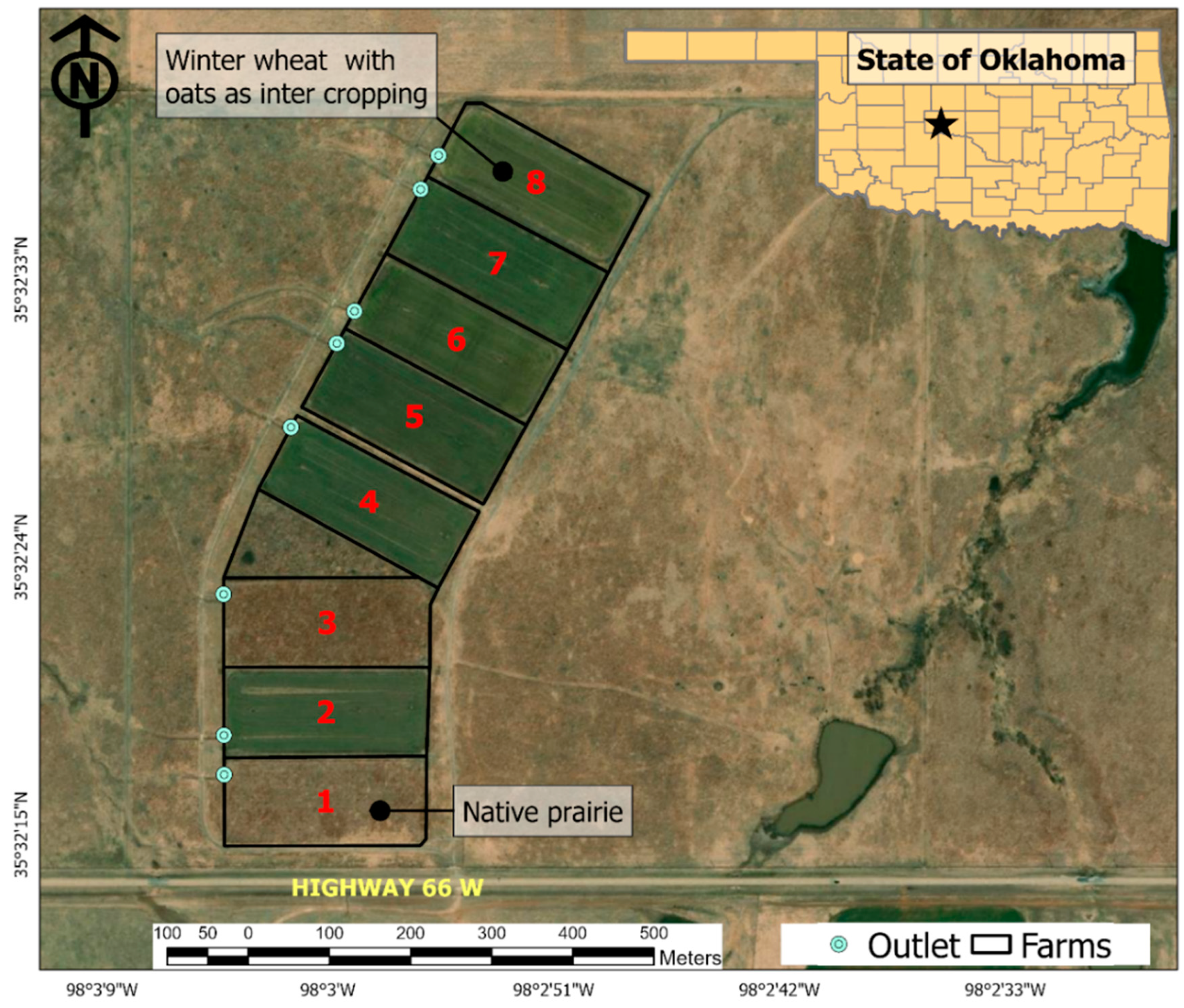
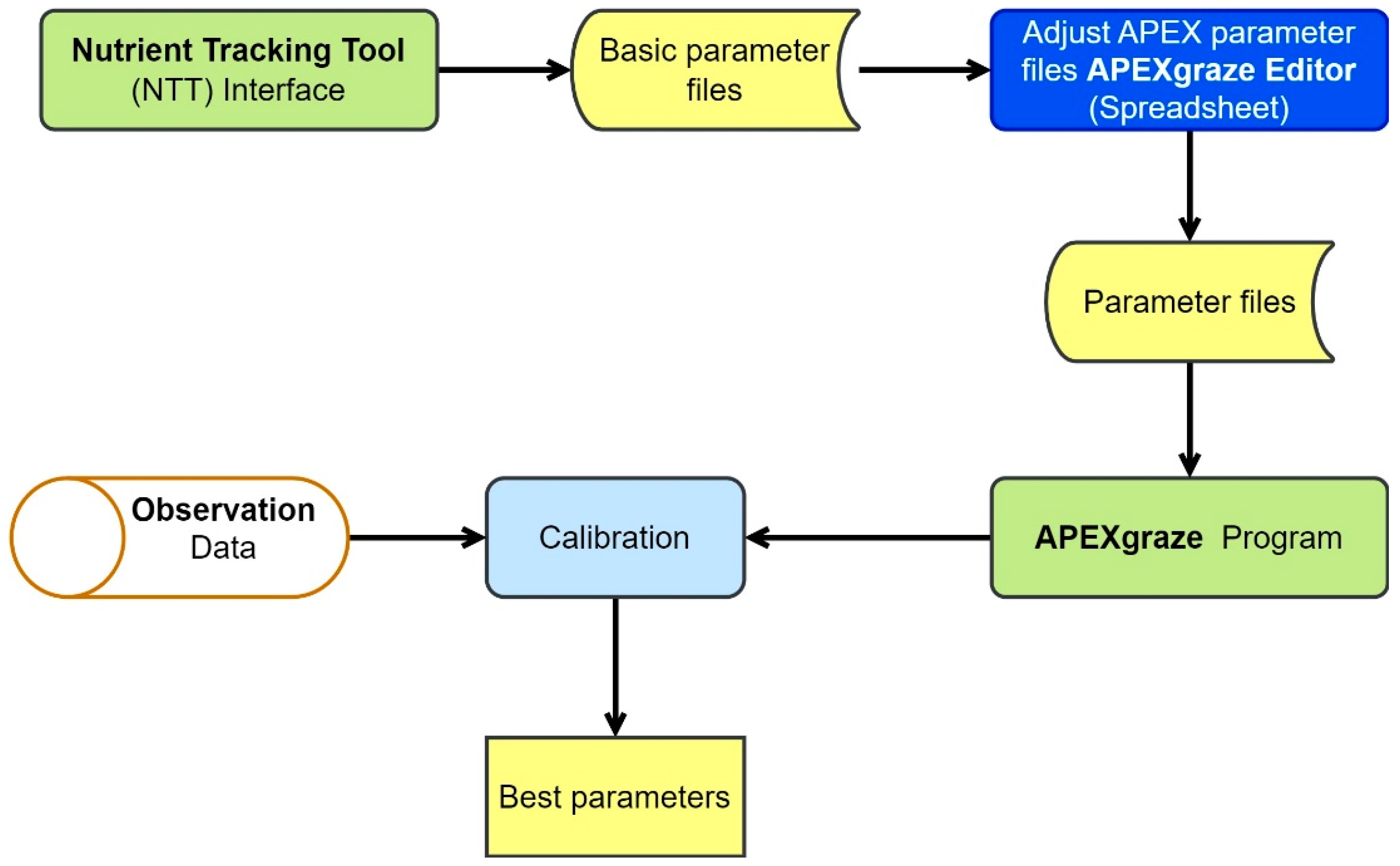
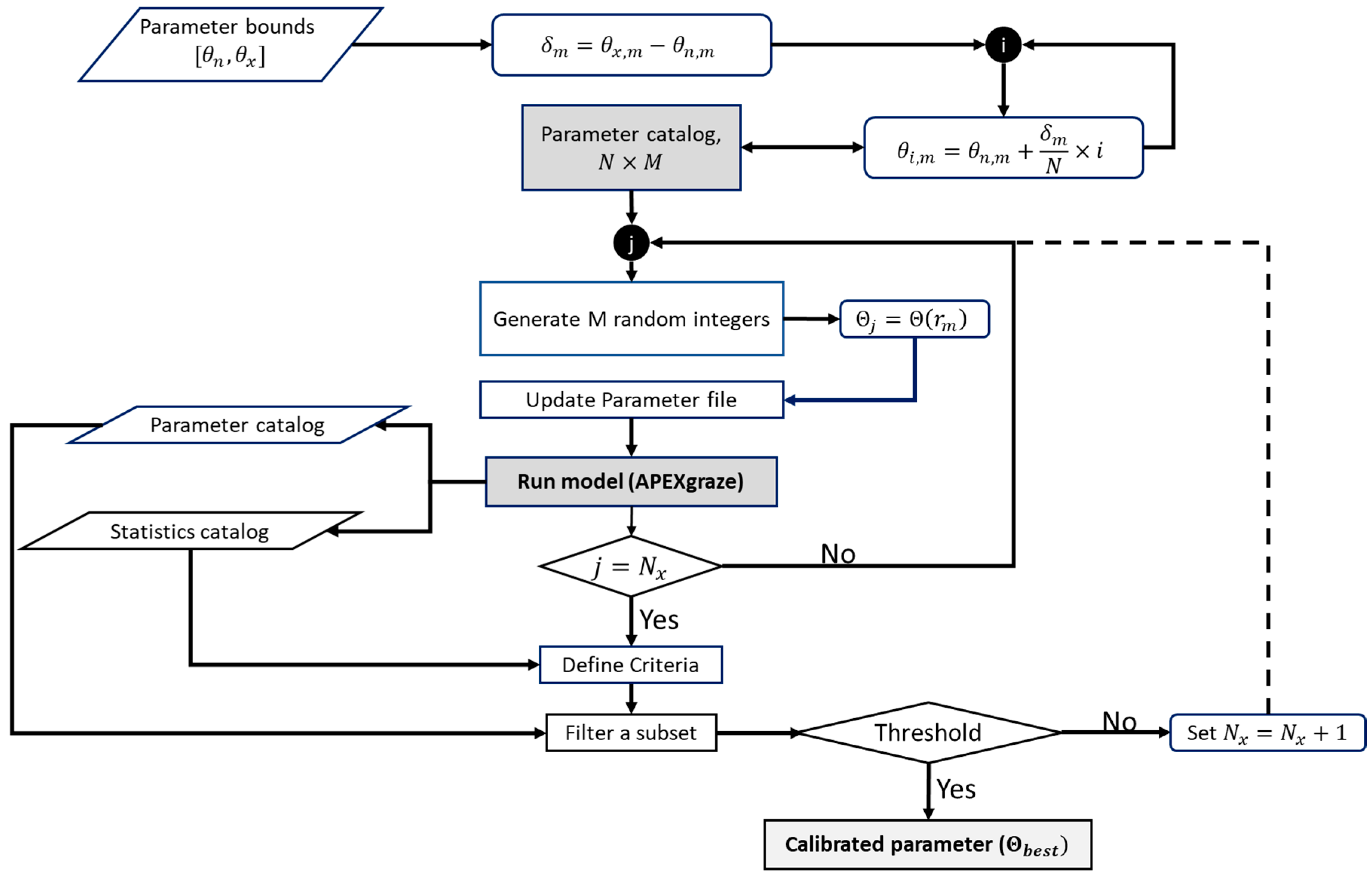
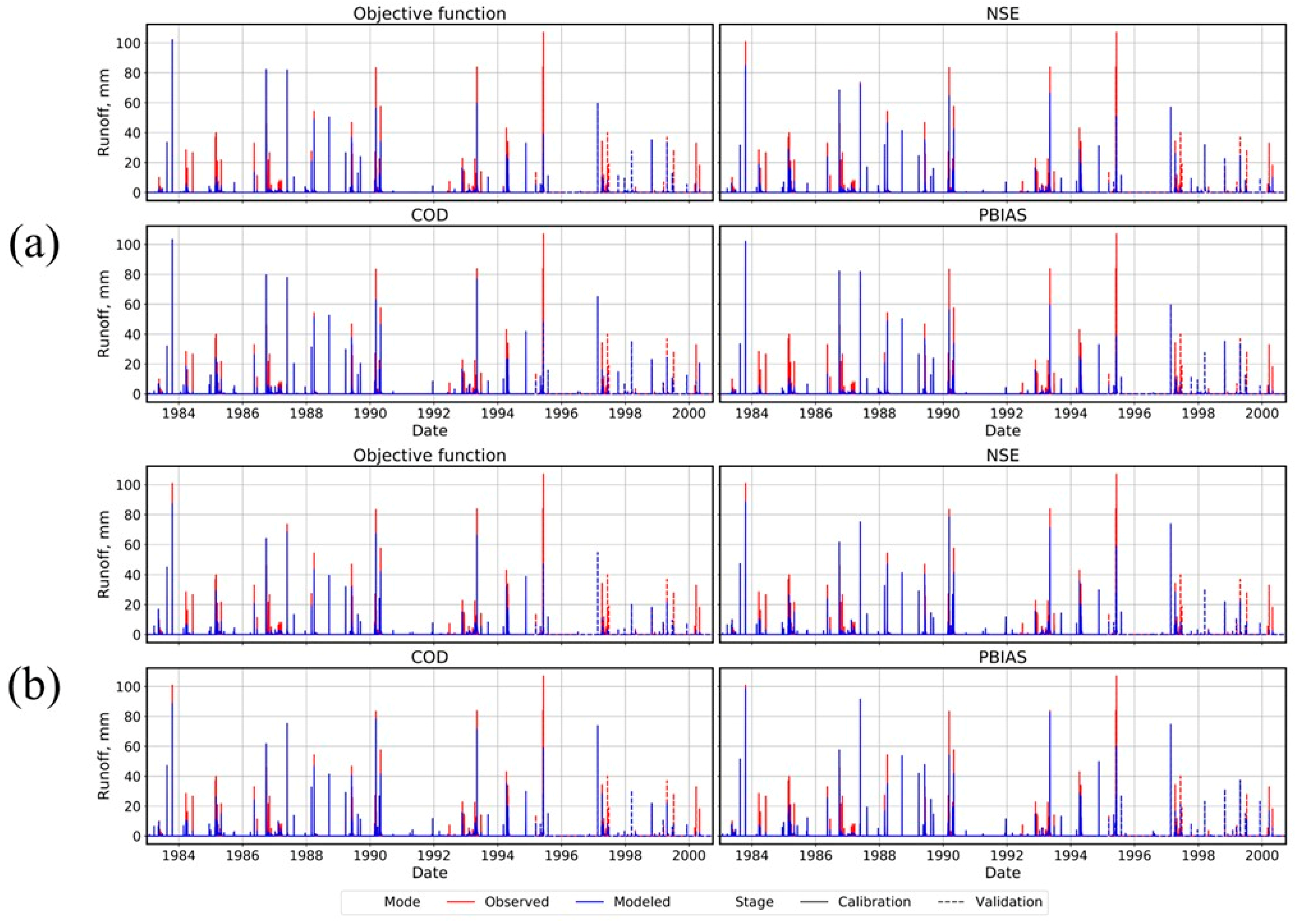
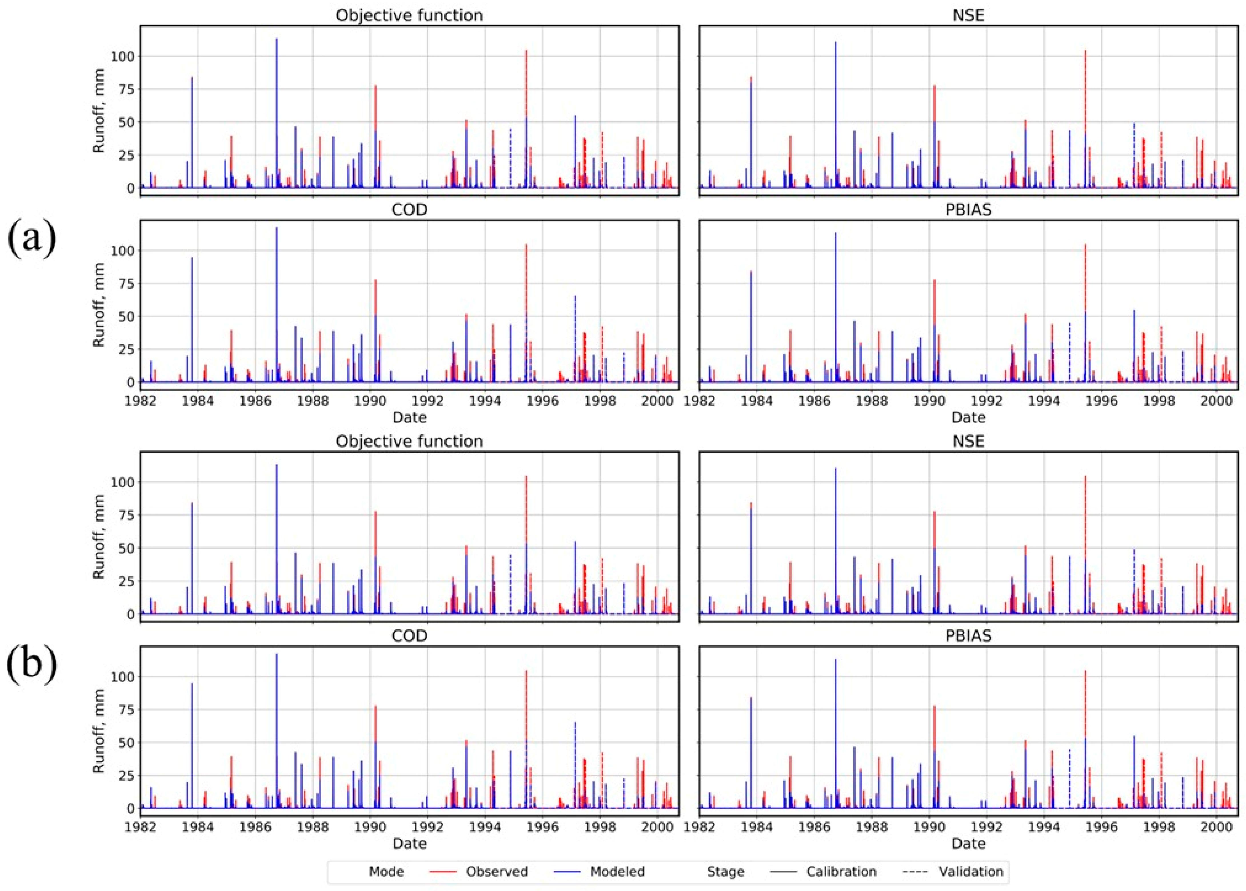
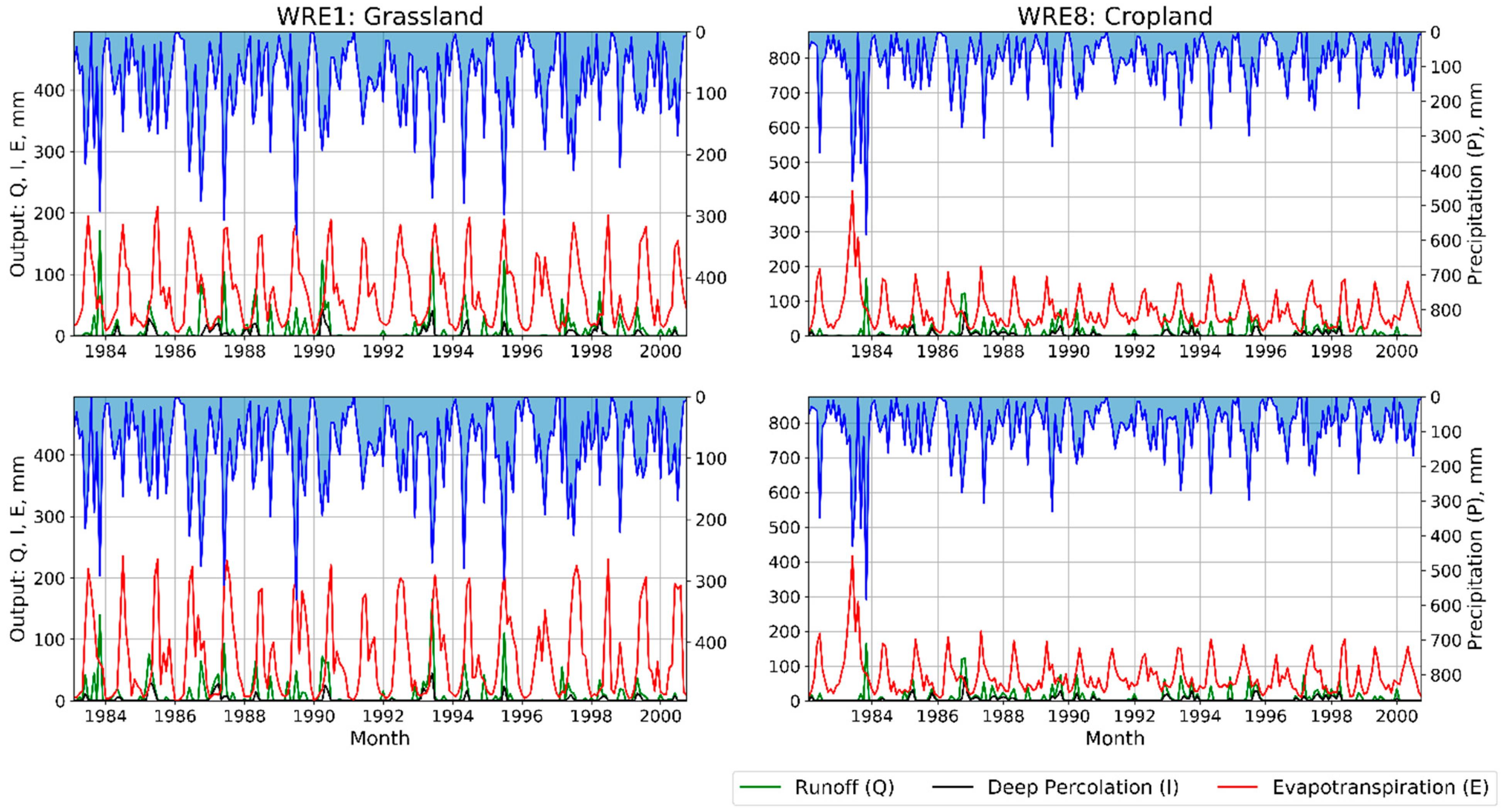
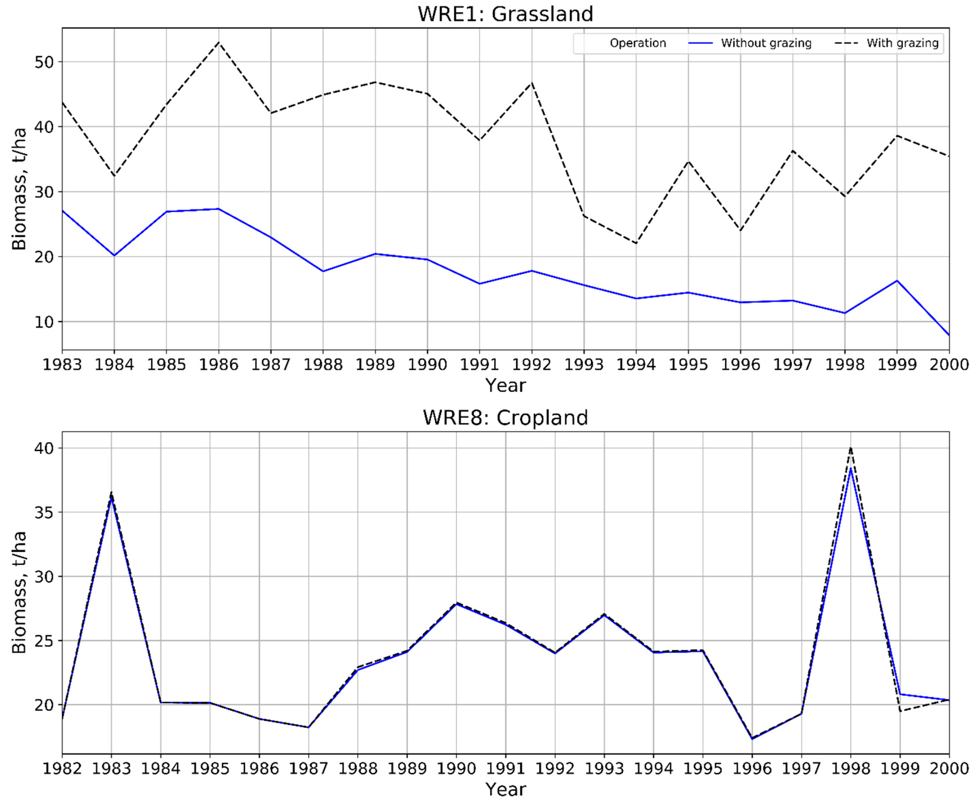
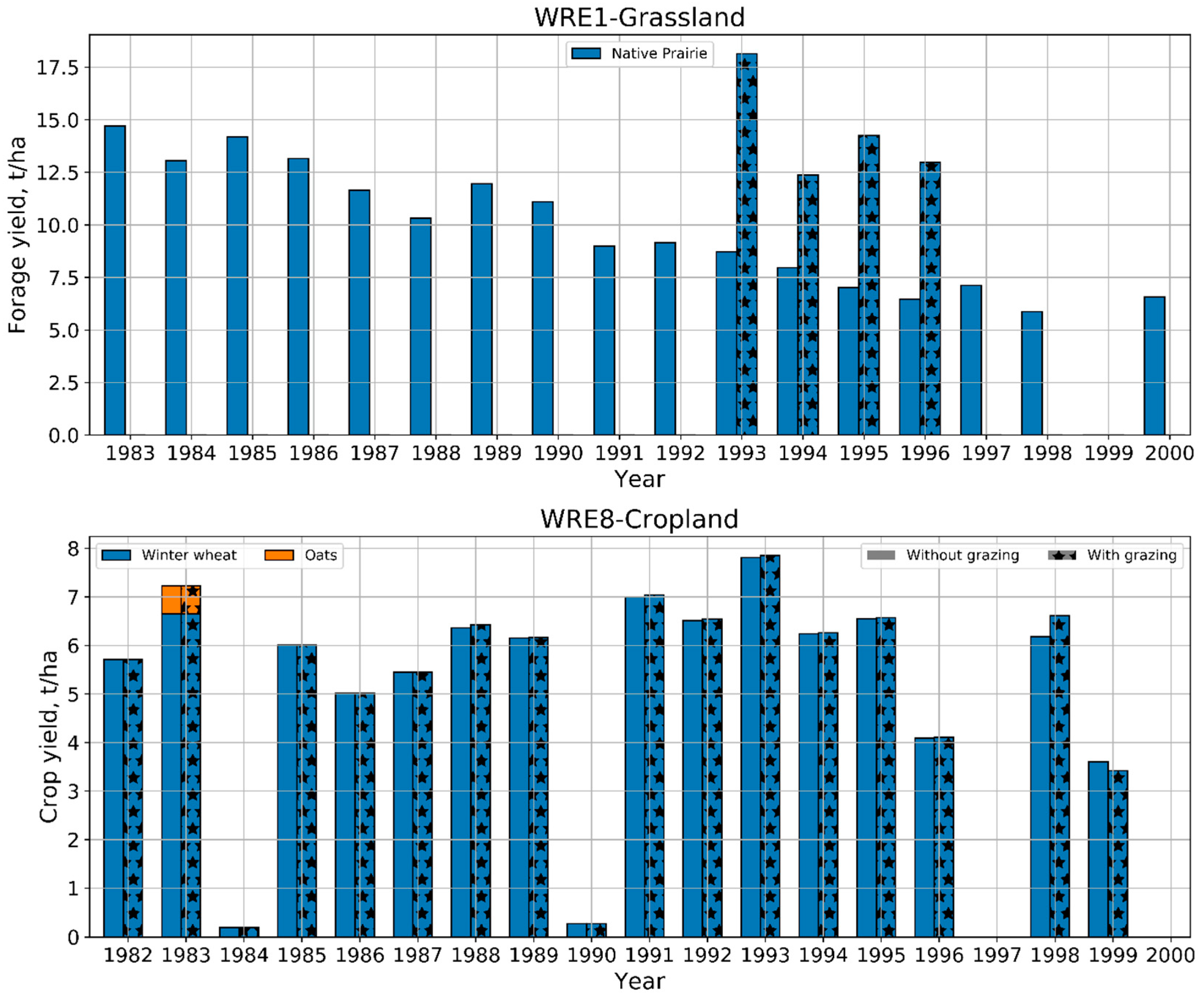
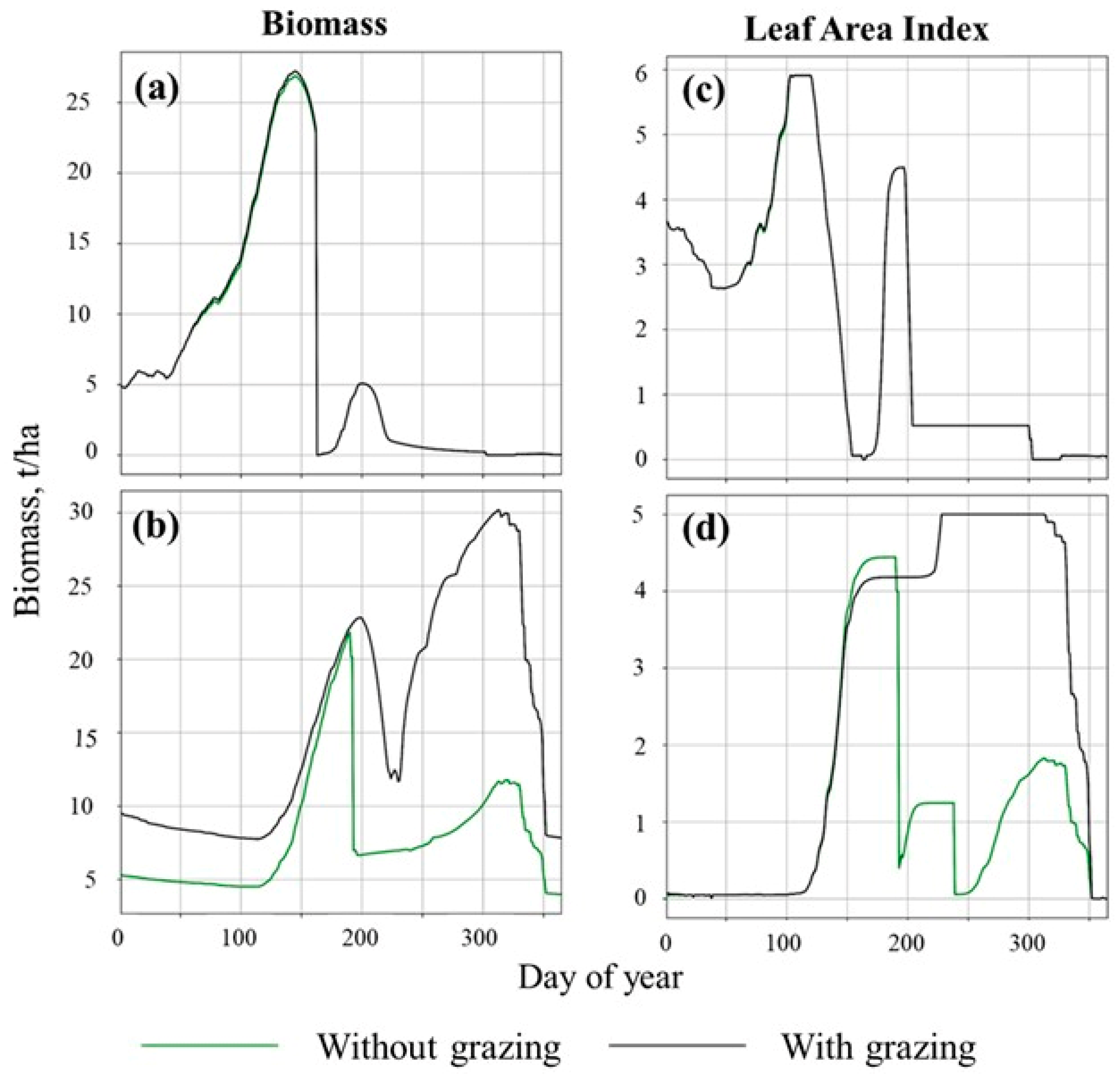
Table 1.
Key information about farm management activities in the two watersheds (1977–2000).
| Activities | WRE1 | WRE8 |
|---|---|---|
| Planting schedules | Once at the very beginning * | 22 times (once a year) |
| Crops | Native prairie | Wheat and oats |
| Total plant population | 3000 plants/m2 | 7289 plants/m2 of wheat and 714 plants/m2 of oats (1983) |
| Number of fertilizer species | 4 | 8 |
| Total fertilizer applied | 706 kg/ha | 4811 kg/ha |
| Number of times fertilizers applied | 2 | 29 |
| Number of pesticide species | 3 | 14 |
| Total pesticides applied | 3 kg/ha | 41 kg/ha |
| Number of times pesticides applied | 2 | 12 |
| Number of classes of cattle that grazed | 3 | 5 |
| Total number of grazed animals | 153 | 100 |
| Total number of days grazed | 620 | 480 |
* Planting date was considered at the very beginning for modeling purposes; it was a pre-established prairie.
Table 2.
Range of key parameters related to surface runoff (hydrology) and sediment, including initial values from the NTT interface, as defined in the user manuals [63,76].
| PARAM (n) | Parameter’s Definition | Lower | Upper | Initial |
|---|---|---|---|---|
| PARAM [2] | Root growth–soil strength | 1 | 2 | 2 |
| PARAM [4] | Water storage N leaching | 0 | 1 | 0.9 |
| PARAM [7] | N fixation | 0 | 1 | 0.9 |
| PARAM [8] | Soluble phosphorus runoff coefficient | 10 | 20 | 20 |
| PARAM [14] | Nitrate leaching ratio | 0.1 | 1 | 0.6 |
| PARAM [15] | Runoff CN residue adjustment parameter | 0 | 0.3 | 0.05 |
| PARAM [17] | Soil evaporation–plant cover factor | 0 | 0.5 | 0.2 |
| PARAM [20] | Runoff curve number initial abstraction | 0.05 | 0.4 | 0.2 |
| PARAM [23] | Hargreaves PET equation coefficient | 0.0023 | 0.0032 | 0.0032 |
| PARAM [34] | Hargreaves PET equation exponent | 0.5 | 0.6 | 0.48 |
| PARAM [42] | SCS curve number index coefficient | 0.3 | 2.5 | 0.8 |
| PARAM [50] | Rainfall interception coefficient | 0.05 | 0.3 | 0.1 |
| PARAM [69] | Coefficient adjusting microbial activity in the topsoil layer | 0.1 | 1 | 1 |
| PARAM [70] | Microbial decay rate coefficient | 0.5 | 1.5 | 1 |
| PARAM [72] | Volatilization/nitrification partitioning coefficient | 0.05 | 0.5 | 0.5 |
| PARAM [18] | Sediment routing exponent | 1 | 2 | 1.5 |
| PARAM [19] | Sediment routing coefficient | 0.0001 | 0.05 | 0 |
| PARAM [45] | Sediment routing travel time coefficient | 0.5 | 10 | 5 |
| PARAM [65] | RUSLE2 transport capacity parameter | 0.001 | 0.1 | 0.001 |
| PARAM [66] | RUSLE2 threshold transport capacity coefficient | 1 | 10 | 1 |
Table 3.
Calibrated APEX parameters for native prairie (WRE1) and cropland (WRE8) for surface runoff, obtained by smallest objective function value. Refer to Table 2 for parameter definitions.
Table 3.
Calibrated APEX parameters for native prairie (WRE1) and cropland (WRE8) for surface runoff, obtained by smallest objective function value. Refer to Table 2 for parameter definitions.
| PARAM (n) | WRE1: Native Prairie | WRE8: Winter Wheat and Oat | ||
|---|---|---|---|---|
| Without Grazing | With Grazing | Without Grazing | With Grazing | |
| PARAM [2] | 1.299 | 1.604 | 1.425 | 1.425 |
| PARAM [4] | 0.327 | 0.220 | 0.724 | 0.724 |
| PARAM [7] | 0.411 | 0.045 | 0.520 | 0.52 |
| PARAM [8] | 17.890 | 10.320 | 18.350 | 18.350 |
| PARAM [14] | 0.335 | 0.783 | 0.699 | 0.699 |
| PARAM [15] | 0.085 | 0.076 | 0.069 | 0.069 |
| PARAM [17] | 0.130 | 0.187 | 0.002 | 0.002 |
| PARAM [18] | 1.325 | 1.463 | 1.303 | 1.303 |
| PARAM [19] | 0.049 | 0.036 | 0.036 | 0.036 |
| PARAM [20] | 0.400 | 0.390 | 0.391 | 0.391 |
| PARAM [23] | 0.0028 | 0.0028 | 0.0029 | 0.0029 |
| PARAM [34] | 0.536 | 0.571 | 0.598 | 0.598 |
| PARAM [42] | 2.447 | 2.212 | 0.828 | 0.828 |
| PARAM [45] | 0.833 | 1.982 | 4.509 | 4.509 |
| PARAM [50] | 0.403 | 0.207 | 0.326 | 0.326 |
| PARAM [65] | 0.022 | 0.039 | 0.086 | 0.086 |
| PARAM [66] | 9.532 | 4.285 | 2.152 | 2.152 |
| PARAM [69] | 0.298 | 0.936 | 0.887 | 0.887 |
| PARAM [70] | 0.595 | 1.201 | 0.871 | 0.871 |
| PARAM [72] | 0.400 | 0.123 | 0.329 | 0.329 |
Table 4.
Model performance for the four best representations shown in Figure 4 and Figure 5, obtained using four statistics: OF: objective function (Equation (2)), NSE: Nash–Sutcliffe efficiency, COD: coefficient of determination, and PBIAS: percent bias in %. Without and with represent the presence or absence of grazing management, respectively. Values inside the parentheses are metrics for validation.
| Watershed | Metrics | OF | NSE | COD | PBIAS, % | ||||
|---|---|---|---|---|---|---|---|---|---|
| Without | With | Without | With | Without | With | Without | With | ||
| WRE1 (Grassland) | OF | 0.66 (4.13) | 0.60 (26.52) | 0.60 (0.16) | 0.66 (0.25) | 0.61 (0.20) | 0.66 (0.26) | 0.00 (3.63) | −0.03 (26.17) |
| NSE | 2.07 (9.71) | 8.80 (1.23) | 0.63 (0.25) | 0.69 (0.23) | 0.64 (0.26) | 0.70 (0.27) | −1.67 (9.32) | −8.46 (0.29) | |
| COD | 6.36 (2.40) | 8.80 (1.23) | 0.62 (0.20) | 0.69 (0.23) | 0.65 (0.24) | 0.70 (0.27) | −6.01 (−1.79) | −8.46 (0.29) | |
| PBIAS | 0.66 (4.13) | 0.64 (4.14) | 0.60 (0.16) | 0.60 (0.21) | 0.61 (0.20) | 0.63 (0.28) | 0.00 (3.63) | 0.00 (3.67) | |
| WRE8 (Cropland) | OF | 30.74 (24.22) | 30.67 (25.10) | 0.67 (0.43) | 0.68 (0.42) | 0.73 (0.43) | 0.73 (0.42) | −30.40 (23.88) | −30.33 (24.75) |
| NSE | 32.61 (22.21) | 32.56 (22.24) | 0.70 (0.37) | 0.70 (0.36) | 0.73 (0.37) | 0.73 (0.36) | −32.27 (21.86) | −32.22 (21.89) | |
| COD | 32.74 (23.16) | 32.73 (22.94) | 0.70 (0.38) | 0.70 (0.39) | 0.76 (0.39) | 0.76 (0.39) | −32.40 (22.81) | −32.39 (22.59) | |
| PBIAS | 30.74 (24.22) | 30.67 (25.10) | 0.67 (0.43) | 0.68 (0.42) | 0.73 (0.43) | 0.73 (0.42) | −30.40 (23.88) | −30.33 (24.75) | |
Table 5.
Summary of response variables averaged annually in grassland (WRE1), implied by four best-calibrated parameter value sets associated with four metrics and respective changes (D) in % after grazing over the simulation period (1983–2000). Shaded cells with positive changes refer to decreased response variables after grazing.
| Response Variables | OF | NSE | COD | PBIAS | ||||
|---|---|---|---|---|---|---|---|---|
| Without | D% | Without | D% | Without | D% | Without | D% | |
| Water yield, mm | 130.59 | 5.9 | 130.29 | −7.5 | 138.31 | −1.2 | 130.59 | −0.01 |
| Deep percolation, mm | 32.07 | 21.6 | 28.22 | 3.4 | 23.77 | −14.7 | 32.07 | 58.9 |
| Sediment, t/ha | 2.21 | 65.2 | 1.87 | 20.1 | 3.25 | 54.1 | 2.21 | 8.3 |
| Soil erosion, t/ha | 2.20 | 65.1 | 1.86 | 19.8 | 3.25 | 54.0 | 2.20 | 8.2 |
| Evapotranspiration, mm | 805.69 | −2.4 | 814.48 | 1.1 | 810.98 | 0.6 | 805.69 | −2.9 |
| Potential ET, mm | 1495.47 | −9.6 | 1741.62 | 8.1 | 1691.97 | 5.4 | 1495.47 | 4.1 |
| Total phosphorus, kg/ha | 0.26 | 48.7 | 0.20 | −40.9 | 0.27 | −4.7 | 0.26 | −25.1 |
| Total nitrogen, kg/ha | 5.17 | 42.0 | 4.93 | 9.9 | 6.20 | 28.3 | 5.17 | −21.8 |
| Plant biomass, t/ha | 13.19 | −98.1 | 14.99 | −18.9 | 10.79 | −65.3 | 13.19 | −23.5 |
| Forage yield, t/ha | 9.33 | 65.6 | 10.79 | 83.2 | 7.58 | 76.1 | 9.33 | 83.7 |
| Standing dead biomass, t/ha | 5.98 | −258.9 | 7.88 | −89.7 | 5.96 | −150.8 | 5.98 | −129.9 |
| Standing live biomass, t/ha | 0.28 | −380.3 | 0.39 | −131.1 | 0.26 | −242.9 | 0.28 | −192.7 |
| Drought stress, d | 6.14 | −530.5 | 22.24 | −19.8 | 16.39 | −62.5 | 6.14 | −283.1 |
| Temperature stress, d | 137.48 | −1.6 | 139.94 | 3.1 | 135.98 | 0.3 | 137.48 | 2.8 |
| Nitrogen stress, d | 76.91 | 98.1 | 23.98 | 8.5 | 0.21 | −100 | 76.91 | 69.9 |
| Phosphorus stress, d | 72.12 | −37.5 | 100.71 | −10.2 | 149.05 | 25.6 | 72.12 | −65.6 |
Table 6.
Summary of response variables, averaged annually in cropland (WRE8), implied by four best-calibrated parameters associated with four metrics and respective changes (D) in % after grazing operations over the simulation period (1982–2000). Shaded cells with positive changes refer to decreased response variables after grazing.
| Response Variables | OF | NSE | COD | PBIAS | ||||
|---|---|---|---|---|---|---|---|---|
| Without | D% | Without | D% | Without | D% | Without | D% | |
| Water yield, mm | 142.33 | 0.4 | 144.86 | 0.04 | 144.46 | −0.1 | 142.33 | 0.4 |
| Deep percolation, mm | 40.27 | −0.4 | 48.29 | −0.9 | 41.24 | 0.3 | 40.27 | −0.4 |
| Sediment, t/ha | 5.92 | 10.3 | 14.85 | 0.4 | 10.46 | −3.4 | 5.92 | 10.3 |
| Soil erosion, t/ha | 5.92 | 10.3 | 14.85 | 0.4 | 10.46 | −3.4 | 5.92 | 10.3 |
| Evapotranspiration, mm | 949.65 | −0.02 | 936.97 | 0.04 | 947.17 | −0.01 | 949.65 | −0.02 |
| Potential ET, mm | 2040.10 | 0.0 | 2002.75 | 0.0 | 2040.10 | 0.0 | 2040.10 | 0.0 |
| Total phosphorus, kg/ha | 2.03 | 7.5 | 4.50 | −0.5 | 3.55 | −3.4 | 2.03 | 7.5 |
| Total nitrogen, kg/ha | 11.97 | 6.4 | 15.35 | −1.0 | 15.53 | −3.4 | 11.97 | 6.4 |
| Crop biomass, t/ha | 19.20 | −0.6 | 18.62 | −0.7 | 20.85 | −0.8 | 19.20 | −0.6 |
| Forage yield, t/ha | 4.27 | −3.0 | 3.77 | −2.1 | 4.56 | −3.7 | 4.27 | −3.0 |
| Standing dead crop residue, t/ha | 13.44 | −0.2 | 13.07 | −0.2 | 14.61 | −0.5 | 13.44 | −0.2 |
| Standing live plant biomass, t/ha | 1.26 | −0.2 | 1.23 | −0.2 | 1.37 | −0.6 | 1.26 | −0.2 |
| Drought stress, d | 4.27 | −3.0 | 3.77 | −2.1 | 4.56 | −3.7 | 4.27 | −3.0 |
| Temperature stress, d | 58.37 | −0.2 | 57.10 | 0.1 | 62.19 | −0.3 | 58.37 | −0.2 |
| Nitrogen stress, d | 18.49 | −0.1 | 22.86 | −0.02 | 1.06 | 11.7 | 18.49 | −0.1 |
| Phosphorus stress, d | - | 0.0 | - | 0.0 | 5.94 | 4.8 | - | 0.0 |
Disclaimer/Publisher’s Note: The statements, opinions and data contained in all publications are solely those of the individual author(s) and contributor(s) and not of MDPI and/or the editor(s). MDPI and/or the editor(s) disclaim responsibility for any injury to people or property resulting from any ideas, methods, instructions or products referred to in the content. |
© 2024 by the authors. Licensee MDPI, Basel, Switzerland. This article is an open access article distributed under the terms and conditions of the Creative Commons Attribution (CC BY) license (https://creativecommons.org/licenses/by/4.0/).
Share and Cite
MDPI and ACS Style
Nelson, A.M.; Maskey, M.L.; Northup, B.K.; Moriasi, D.N. Calibrating Agro-Hydrological Model under Grazing Activities and Its Challenges and Implications. Hydrology 2024, 11, 42. https://0-doi-org.brum.beds.ac.uk/10.3390/hydrology11040042
AMA Style
Nelson AM, Maskey ML, Northup BK, Moriasi DN. Calibrating Agro-Hydrological Model under Grazing Activities and Its Challenges and Implications. Hydrology. 2024; 11(4):42. https://0-doi-org.brum.beds.ac.uk/10.3390/hydrology11040042
Chicago/Turabian StyleNelson, Amanda M., Mahesh L. Maskey, Brian K. Northup, and Daniel N. Moriasi. 2024. "Calibrating Agro-Hydrological Model under Grazing Activities and Its Challenges and Implications" Hydrology 11, no. 4: 42. https://0-doi-org.brum.beds.ac.uk/10.3390/hydrology11040042
Note that from the first issue of 2016, this journal uses article numbers instead of page numbers. See further details here.