
A Temporal Fusion Transformer Model to Forecast Overflow from Sewer Manholes during Pluvial Flash Flood Events


Abstract
:1. Introduction
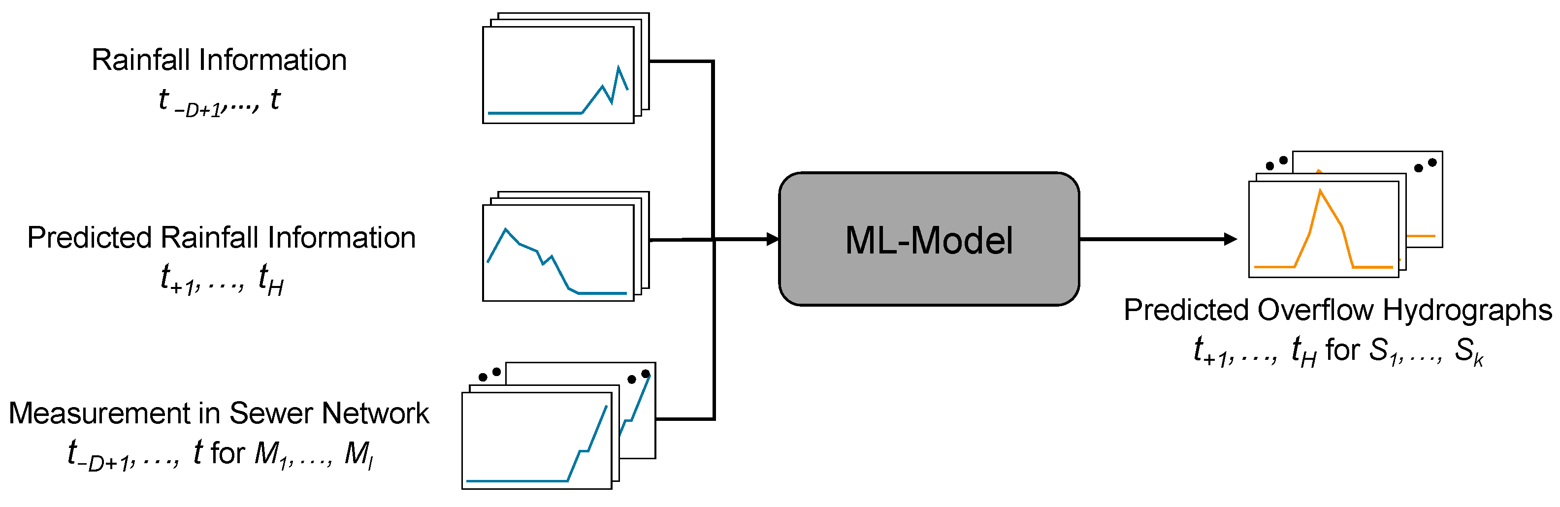
- Evaluation of a deep learning-based model capable of forecasting overflow hydrographs at the manhole level. In contrast to other studies, the temporal fusion transformer [31] as a transformer-based network architecture is used. Transformers have proven to be very efficient in processing sequences, and in the case of the temporal fusion transformer, especially in the field of time series analysis and forecasting.
- The influence of a spatially high-resolution sensor network as an additional input variable on the accuracy of the prediction results is evaluated. This approach is compared to a model considering only one sensor at the outlet of the sewer network and a model without measurements in the sewer network.
- The influence of the selected measurement signal on the prediction quality is tested. Signals considered for which the performance of the trained models is evaluated are discharge, water level, filling degree and filling level classes.
2. Methodology
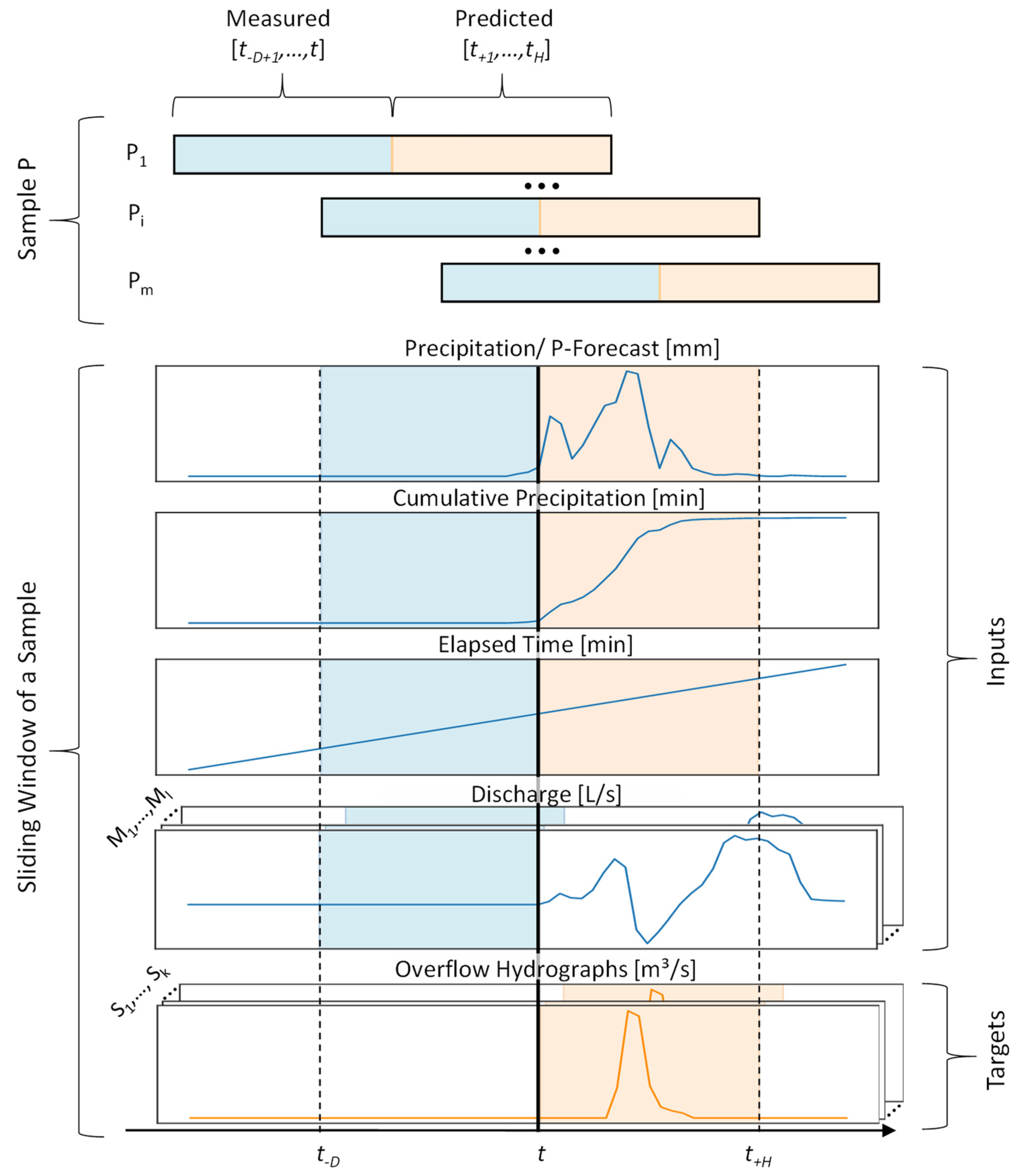
2.1. Model Setup
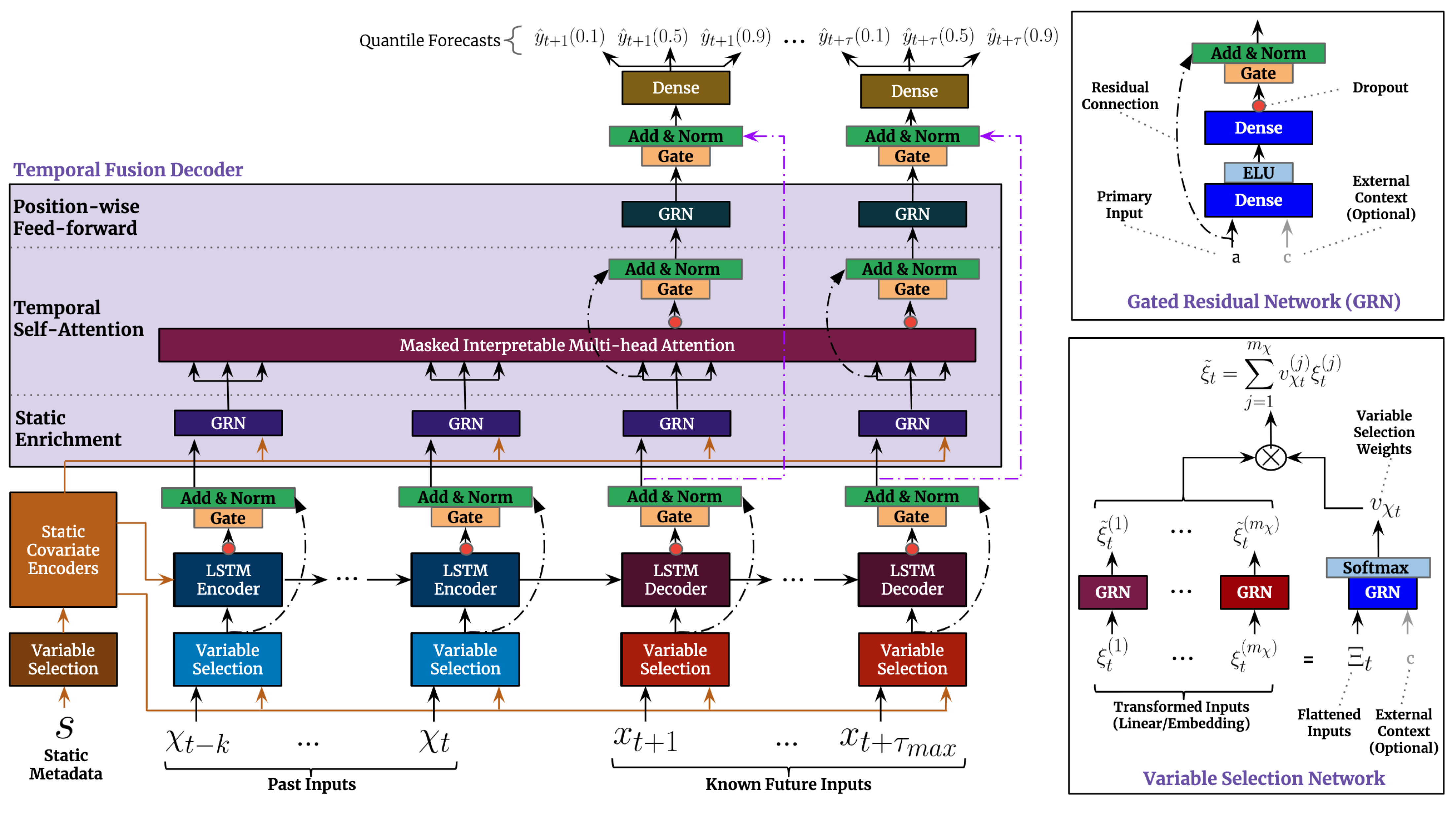
2.2. Temporal Fusion Transformer
3. Case Study
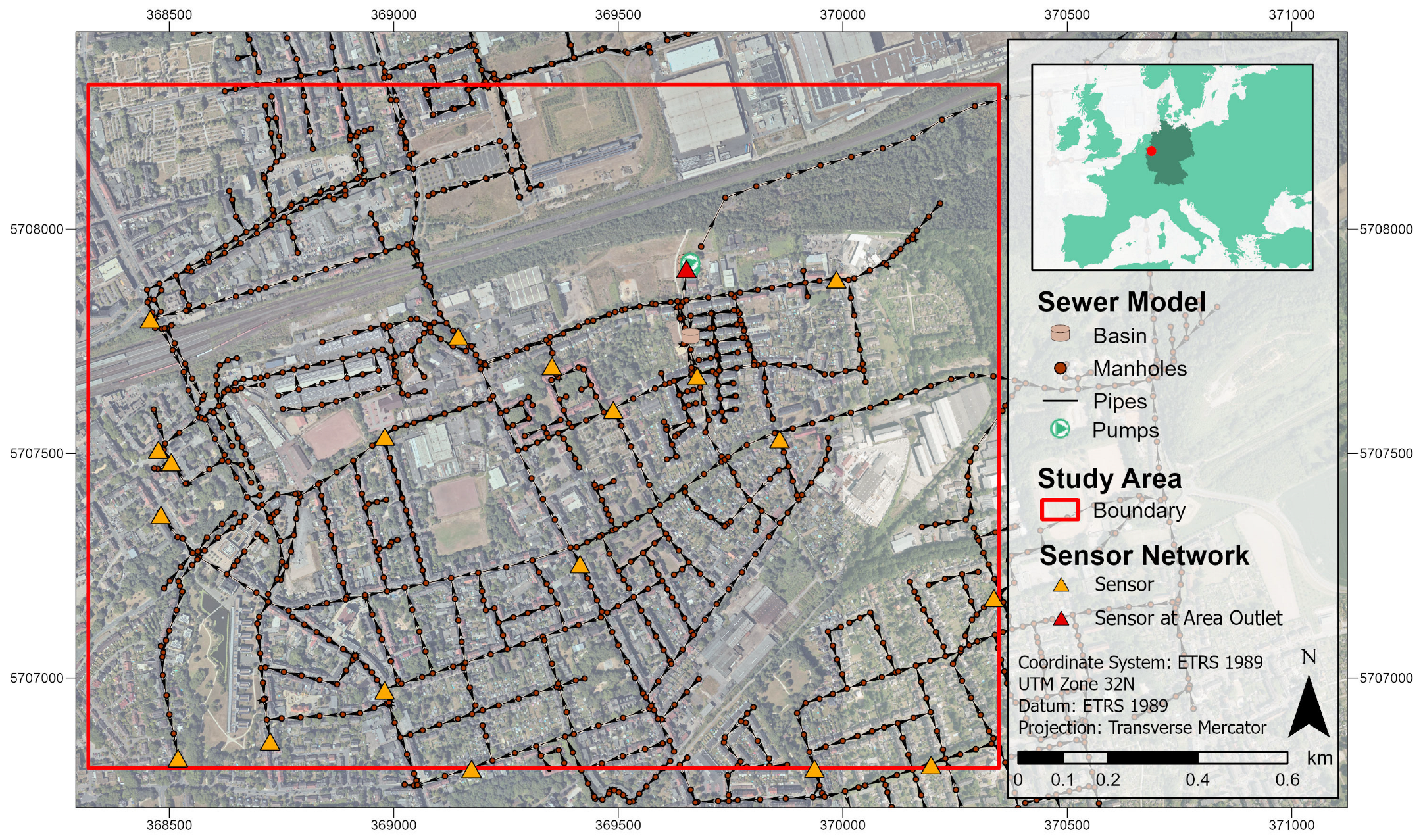
3.1. Study Area and Monitoring Network
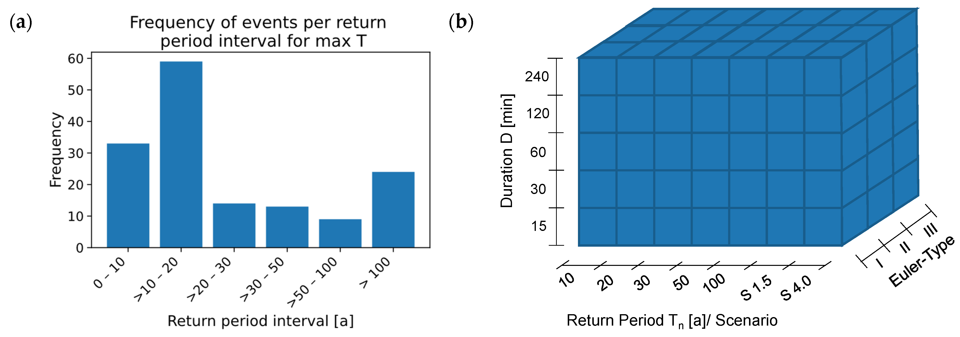
3.2. Data Generation and Preprocessing
3.3. Experiments
3.3.1. Comparison with Different Deep Learning Models
- CNN: Convolutional neural networks are a network architecture developed significantly through the work of Le Cun et al. [44], which has proven to be highly effective in image recognition. In addition to processing 2D data such as images, CNNs can also process 1D datasets such as time series. CNNs focus on recognising relevant structures in input data, and are therefore able to localise short-term dependencies and local patterns. In the present use case, the patterns extracted from the input time series are then used to generate the overflow forecast for the upcoming time steps with a fully connected feed-forward layer.
- LSTM Network: Models using the LSTM cells developed by Hochreiter and Schmidhuber [45] are widely used in the field of time series analysis. They are a type of recurrent neural network (RNN), but have additional modifications that make it possible to learn long-term dependencies in sequences, which makes them well-suited for the prediction of time series. Like the CNN model, the LSTM model used here has a fully connected feed-forward layer as an output layer to generate a multi-step prediction.
- Seq2Seq: The Seq2Seq model presented by Sutskever et al. [46] represents a network architecture for processing sequential data that also includes recurrent layers. In contrast to the LSTM model described before, the recurrent layers are arranged in an encoder–decoder structure. The encoder processes the inputs and generates a context vector, while the decoder produces an output sequence based on this vector. Furthermore, Seq2Seq models can provide predictions for several time steps without requiring additional feed-forward layers. LSTM cells are also used as recurrent layers in the Seq2Seq model used in this work.
- DA-RNN: A DA-RNN comprises a Seq2Seq model supplemented with a two-stage attention mechanism [47]. These attention mechanisms are placed before and after the encoder, and similarly to the TFT, are used to consider all time steps of the input sequences and to weight them depending on their influence on the prediction result.
3.3.2. Analyses with Measurements in the Sewer Network
3.4. Performance Evaluation
4. Results
4.1. Evaluation of the Analyses Performed
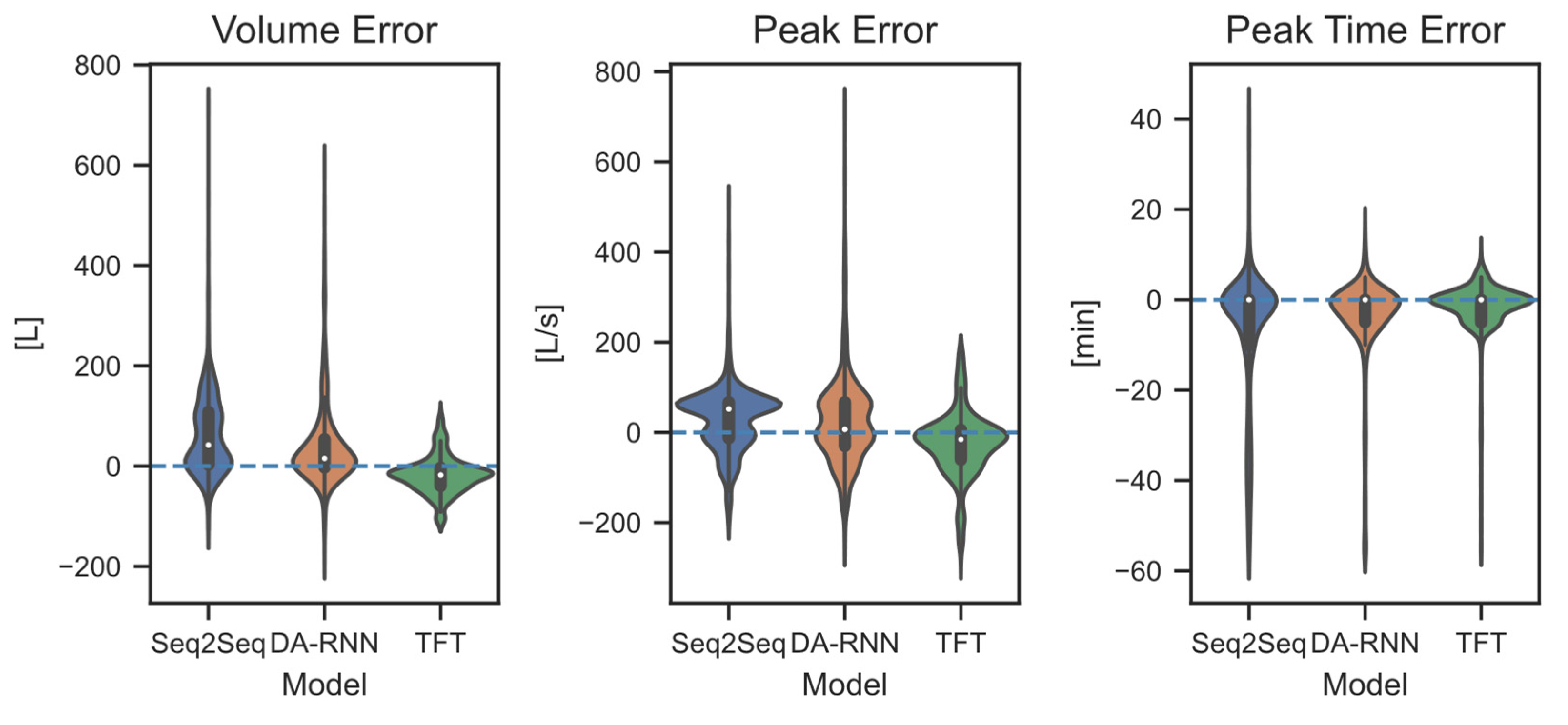
- Comparison of model architectures: The comparison of the different model architectures shows that the naïve approach, as well as the CNN and LSTM, deliver significantly worse forecasts than the other model architectures. In some cases, CNN and LSTM even show worse results than the naïve approach. Even if the TFT does not perform best across all the considered variants, a TFT model achieves the best overall result for each metric. However, the results for the Seq2Seq model and the TFT are usually close to each other.
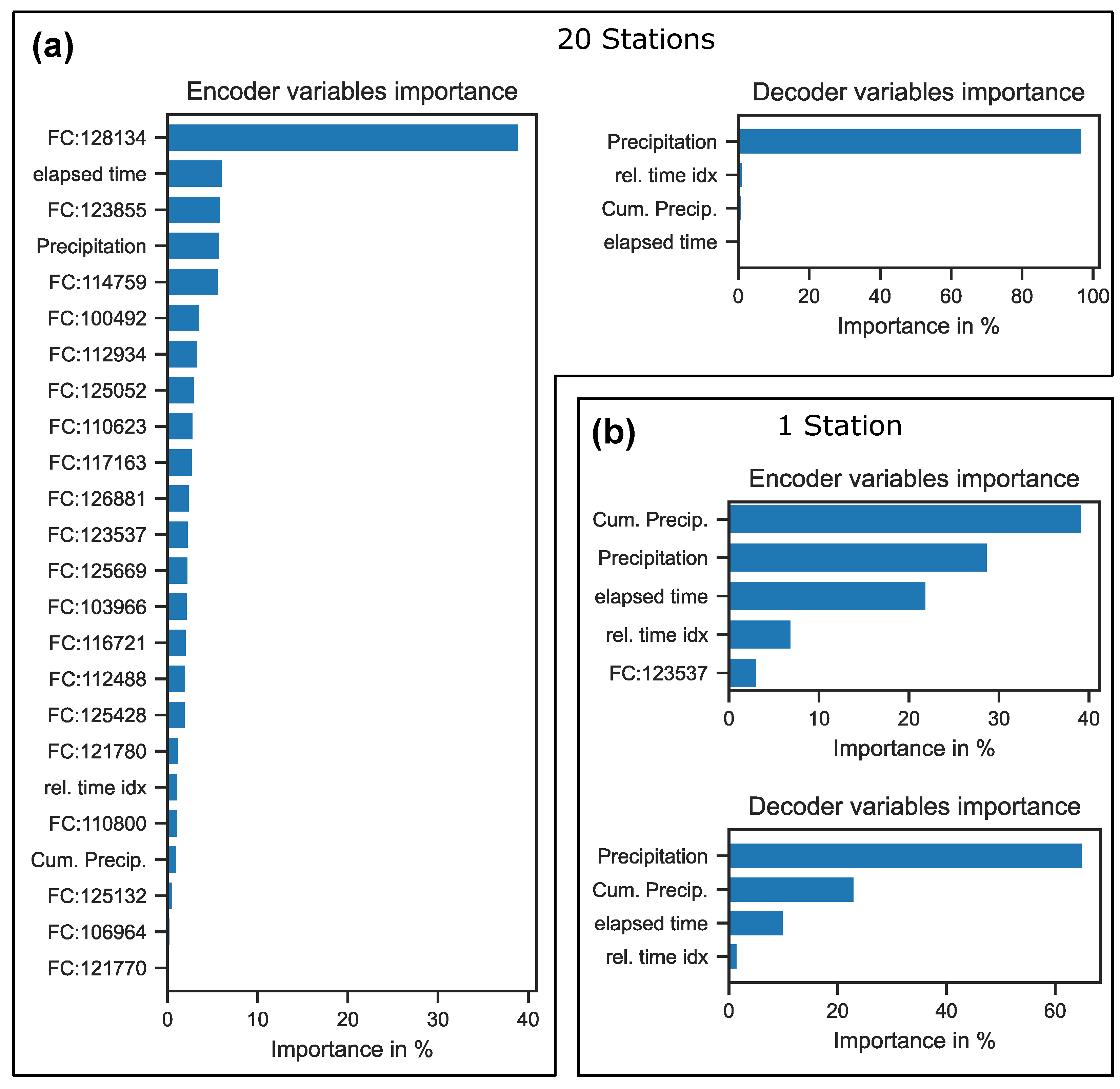
- Comparison of the number of sensors: A larger number of sensors does not have a positive influence on the results, as the variants with 20 sensors tended to achieve poorer results. The variants with one sensor and no sensor, on the other hand, are close to each other in most cases. The best overall results for all three metrics were achieved for a variant with one sensor.
- Comparison of measurement signals: No clear tendency towards one variable can be recognised for the measurement signals considered. In the variants with one station, only the results for the water level stand out negatively for the two best model architectures—Seq2Seq and TFT. The lowest volume error and the lowest peak time error were achieved when measuring the filling degree. The lowest peak error was obtained by the approach with five filling classes.

| Model | 20 Stations | 1 Station | No Station | ||||||
|---|---|---|---|---|---|---|---|---|---|
| VE [L] | PE [L/s] | PTE [min] | VE [L] | PE [L/s] | PTE [min] | VE [L] | PE [L/s] | PTE [min] | |
| Discharge | |||||||||
| Naïve Zero | 138.65 | 199.30 | 27.50 | 138.65 | 199.30 | 27.50 | 138.65 | 199.30 | 27.50 |
| CNN | 235.58 | 148.54 | 20.32 | 228.65 | 169.03 | 25.51 | 208.87 | 152.20 | 20.70 |
| LSTM | 147.61 | 179.65 | 10.55 | 174.80 | 246.92 | 7.84 | 169.46 | 181.34 | 7.84 |
| Seq2Seq | 90.73 | 85.41 | 7.13 | 49.07 | 83.81 | 5.96 | 50.51 | 74.04 | 6.12 |
| DA-RNN | 133.41 | 154.09 | 5.08 | 85.79 | 99.92 | 6.11 | 96.08 | 112.13 | 8.01 |
| TFT | 92.84 | 136.83 | 15.82 | 44.25 | 79.77 | 2.53 | 61.13 | 91.45 | 4.04 |
| Water depth | |||||||||
| Naïve Zero | 138.65 | 199.30 | 27.50 | 138.65 | 199.30 | 27.50 | 138.65 | 199.30 | 27.50 |
| CNN | 200.96 | 137.53 | 22.10 | 259.23 | 154.80 | 22.07 | 208.87 | 152.20 | 20.70 |
| LSTM | 157.30 | 170.15 | 8.20 | 137.15 | 178.62 | 9.29 | 169.46 | 181.34 | 7.84 |
| Seq2Seq | 77.10 | 76.65 | 5.18 | 89.24 | 96.58 | 4.03 | 50.51 | 74.04 | 6.12 |
| DA-RNN | 101.18 | 117.02 | 4.52 | 62.94 | 84.53 | 7.34 | 96.08 | 112.13 | 8.01 |
| TFT | 62.05 | 101.91 | 2.12 | 57.76 | 101.35 | 2.64 | 61.13 | 91.45 | 4.04 |
| Filling degree | |||||||||
| Naïve Zero | 138.65 | 199.30 | 27.50 | 138.65 | 199.30 | 27.50 | 138.65 | 199.30 | 27.50 |
| CNN | 225.52 | 160.67 | 19.54 | 270.09 | 168.48 | 26.15 | 208.87 | 152.20 | 20.70 |
| LSTM | 147.70 | 168.95 | 10.29 | 157.77 | 184.91 | 7.36 | 169.46 | 181.34 | 7.84 |
| Seq2Seq | 97.99 | 98.01 | 9.56 | 43.39 | 90.01 | 2.16 | 50.51 | 74.04 | 6.12 |
| DA-RNN | 80.77 | 100.03 | 4.58 | 108.75 | 103.39 | 8.65 | 96.08 | 112.13 | 8.01 |
| TFT | 43.19 | 78.49 | 3.10 | 36.93 | 77.42 | 2.07 | 61.13 | 91.45 | 4.04 |
| Filling class (5 classes) | |||||||||
| Naïve Zero | 138.65 | 199.30 | 27.50 | 138.65 | 199.30 | 27.50 | 138.65 | 199.30 | 27.50 |
| CNN | 271.46 | 171.68 | 19.61 | 300.05 | 178.35 | 25.37 | 208.87 | 152.20 | 20.70 |
| LSTM | 151.27 | 170.61 | 10.43 | 160.64 | 176.63 | 6.67 | 169.46 | 181.34 | 7.84 |
| Seq2Seq | 78.38 | 91.00 | 10.31 | 59.15 | 78.35 | 4.08 | 50.51 | 74.04 | 6.12 |
| DA-RNN | 102.93 | 126.97 | 7.80 | 65.84 | 93.26 | 5.05 | 96.08 | 112.13 | 8.01 |
| TFT | 86.68 | 125.77 | 4.90 | 44.25 | 73.72 | 2.71 | 61.13 | 91.45 | 4.04 |
4.2. Forecast for a Historical Heavy Rainfall Event
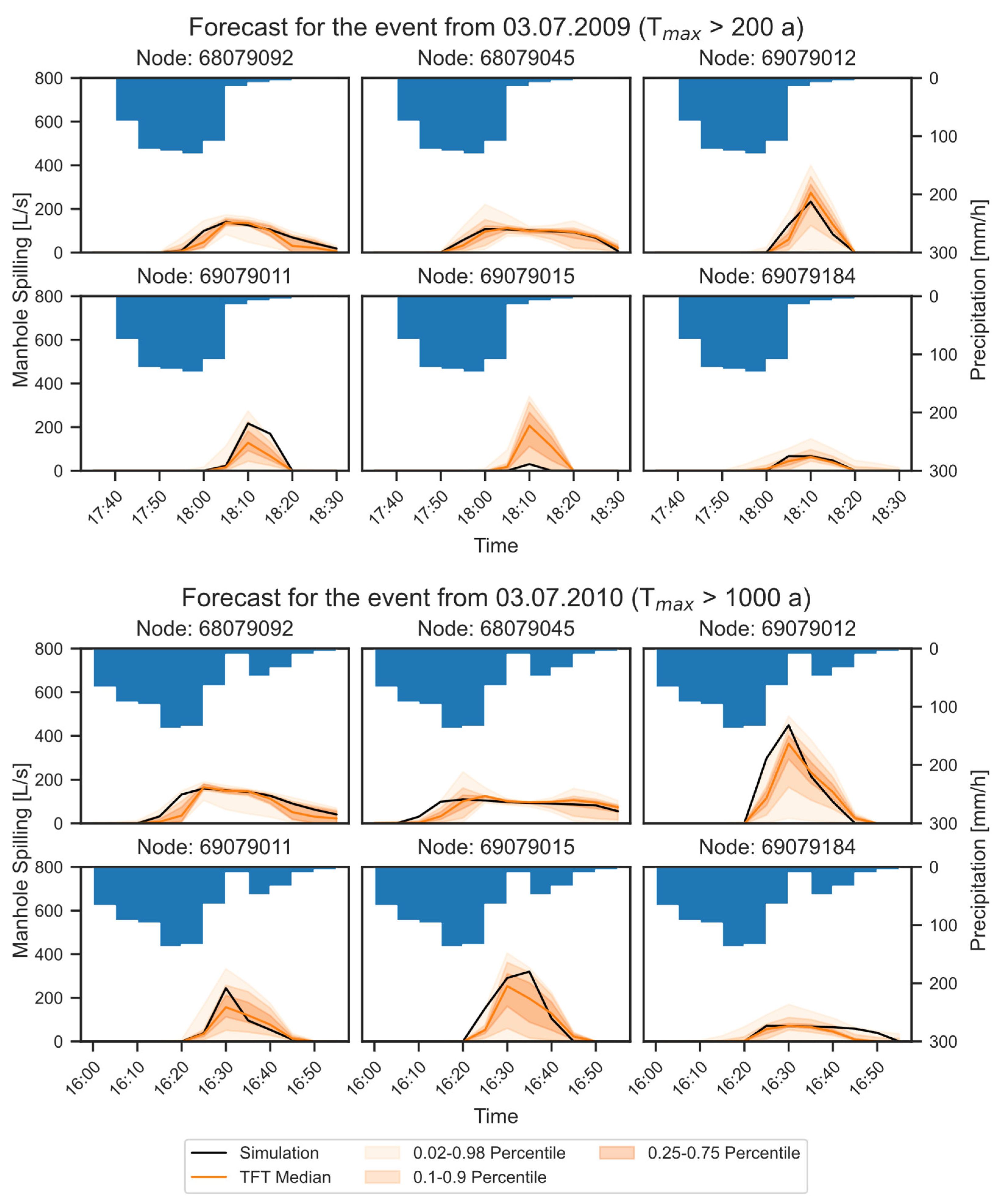
- In some cases, the 0.5 quantile matches the simulated target value very well, but there are also significant deviations in other cases. In addition, the uncertainty range between the 0.02 and 0.98 quantiles increases with larger deviations.
- Longer overflow events can be predicted with high accuracy, while short peaks can result in extreme deviations of >100% at the maximum value and of the resulting overflow volume. This is particularly illustrated in the forecast hydrographs for the event of 3 July 2009. While the longer overflow period at nodes 68079092 and 68079045 is forecast with a high degree of accuracy, the hydrograph for the short peak at node 69079015 deviates significantly.
- In this figure, there is no recognisable tendency of the model to consistently under- or overestimate overflow hydrographs at the manholes shown. This finding can also be confirmed after analyses of other manholes in the catchment area, which are not shown here.

5. Discussion
6. Conclusions
- The optimisation of the final model with regard to the forecast of overflow hydrographs with short peaks. On the one hand, this can be achieved by considering further input features or a larger training dataset. On the other hand, testing with other network architectures, such as graph neural networks or different types of transformer models, could be helpful. In addition, further optimisation to improve the accuracy of the final model could be attempted with the implementation of systematic hyperparameter tuning.
- Investigations on the coupled assessment of real measurement networks and the forecast models for precipitation, overflow and flooded areas. The first step is to evaluate the performance of the coupled forecasting system itself. In addition, it is also necessary to test alternatives for ensuring that the uncertainties of the individual components in the forecasting process are adequately taken into account and visualised.
- Establishing the model’s scalability for broad application at urban-area level is also necessary. One possibility for this could be the use of physically informed or physically guided neural networks, which, if set up appropriately, allow transferability to other areas.
Author Contributions
Funding
Data Availability Statement
Acknowledgments
Conflicts of Interest
References
- Seneviratne, S.I.; Zhang, X.; Adnan, M.; Badi, W.; Dereczynski, C.; Di Luca, A.; Ghosh, S.; Iskandar, I.; Kossin, J.; Lewis, S.; et al. Weather and Climate Extreme Events in a Changing Climate. In Climate Change 2021: The Physical Science Basis. Contribution of Working Group I to the Sixth Assessment Report of the Intergovernmental Panel on Climate Change; Masson-Delmotte, V., Zhai, P., Pirani, A., Connors, S.L., Péan, C., Berger, S., Caud, N., Chen, Y., Goldfarb, L., Gomis, M.I., et al., Eds.; Cambridge University Press: Cambridge, UK; New York, NY, USA, 2021; pp. 1513–1766. [Google Scholar]
- Tradowsky, J.S.; Philip, S.Y.; Kreienkamp, F.; Kew, S.F.; Lorenz, P.; Arrighi, J.; Bettmann, T.; Caluwaerts, S.; Chan, S.C.; de Cruz, L.; et al. Attribution of the heavy rainfall events leading to severe flooding in Western Europe during July 2021. Clim. Change 2023, 176, 90. [Google Scholar] [CrossRef]
- Zachariah, M.; Kotroni, V.; Kostas, L.; Barnes, C.; Kimutai, J.; Kew, S.; Pinto, I.; Yang, W.; Vahlberg, M.; Singh, R.; et al. Interplay of Climate Change—Exacerbated Rainfall, Exposure and Vulnerability Led to Widespread Impacts in the Mediterranean Region; World Weather Attribution, Grantham Institute for Climate Change: London, UK, 2023. [Google Scholar]
- DIN EN 752:2017; Entwässerungssysteme außerhalb von Gebäuden—Kanalmanagement. Deutsches Institut für Normung e.V.: Berlin, Germany; Beuth Verlag GmbH: Berlin, Germany, 2017.
- Henonin, J.; Russo, B.; Mark, O.; Gourbesville, P. Real-time urban flood forecasting and modelling—A state of the art. J. Hydroinf. 2013, 15, 717–736. [Google Scholar] [CrossRef]
- Faure, D.; Schmitt, P.; Auchet, P. Limits of radar rainfall forecasting for sewage system management: Results and application in Nancy. In Proceedings of the 8th International Conference on Urban Storm Drainage, Sydney, Australia, 30 August 1999. [Google Scholar]
- Quirmbach, M. Nutzung von Wetterradardaten für Niederschlags-und Abflussvorhersagen in Urbanen Einzugsgebieten. Ph.D. Thesis, Lehrstuhl für Hydrologie, Wasserwirtschaft und Umwelttechnik, Ruhr-Universität Bochum, Bochum, Germany, 2003. [Google Scholar]
- Jasper-Tönnies, A.; Hellmers, S.; Einfalt, T.; Strehz, A.; Fröhle, P. Ensembles of radar nowcasts and COSMO-DE-EPS for urban flood management. Water Sci. Technol. 2018, 2017, 27–35. [Google Scholar] [CrossRef] [PubMed]
- René, J.-R.; Djordjević, S.; Butler, D.; Mark, O.; Henonin, J.; Eisum, N.; Madsen, H. A real-time pluvial flood forecasting system for Castries, St. Lucia. J. Flood Risk Manag. 2015, 11, 269–283. [Google Scholar] [CrossRef]
- Bates, P.D.; Horritt, M.S.; Fewtrell, T.J. A simple inertial formulation of the shallow water equations for efficient two-dimensional flood inundation modelling. J. Hydrol. 2010, 387, 33–45. [Google Scholar] [CrossRef]
- Austin, R.J.; Chen, A.S.; Savić, D.A.; Djordjević, S. Quick and accurate Cellular Automata sewer simulator. J. Hydroinf. 2014, 16, 1359–1374. [Google Scholar] [CrossRef]
- Jamali, B.; Löwe, R.; Bach, P.M.; Urich, C.; Arnbjerg-Nielsen, K.; Deletic, A. A rapid urban flood inundation and damage assessment model. J. Hydrol. 2018, 564, 1085–1098. [Google Scholar] [CrossRef]
- Mosavi, A.; Ozturk, P.; Chau, K. Flood Prediction Using Machine Learning Models: Literature Review. Water 2018, 10, 1536. [Google Scholar] [CrossRef]
- Bentivoglio, R.; Isufi, E.; Jonkman, S.N.; Taormina, R. Deep Learning Methods for Flood Mapping: A Review of Existing Applications and Future Research Directions. Hydrol. Earth Syst. Sci. 2022, 26, 4345–4378. [Google Scholar] [CrossRef]
- Berkhahn, S.; Fuchs, L.; Neuweiler, I. An ensemble neural network model for real-time prediction of urban floods. J. Hydrol. 2019, 575, 743–754. [Google Scholar] [CrossRef]
- Guo, Z.; Leitão, J.P.; Simões, N.E.; Moosavi, V. Data-driven flood emulation: Speeding up urban flood predictions by deep convolutional neural networks. J. Flood Risk Manag. 2020, 14, e12684. [Google Scholar] [CrossRef]
- Löwe, R.; Böhm, J.; Jensen, D.G.; Leandro, J.; Rasmussen, S.H. U-FLOOD—Topographic deep learning for predicting urban pluvial flood water depth. J. Hydrol. 2021, 603, 126898. [Google Scholar] [CrossRef]
- Hofmann, J.; Schüttrumpf, H. floodGAN: Using Deep Adversarial Learning to Predict Pluvial Flooding in Real Time. Water 2021, 13, 2255. [Google Scholar] [CrossRef]
- do Lago, C.A.; Giacomoni, M.H.; Bentivoglio, R.; Taormina, R.; Gomes, M.N.; Mendiondo, E.M. Generalizing rapid flood predictions to unseen urban catchments with conditional generative adversarial networks. J. Hydrol. 2023, 618, 129276. [Google Scholar] [CrossRef]
- Garzón, A.; Kapelan, Z.; Langeveld, J.; Taormina, R. Machine Learning-Based Surrogate Modeling for Urban Water Networks: Review and Future Research Directions. Water Resour. Res. 2022, 58, e2021WR031808. [Google Scholar] [CrossRef]
- Chang, F.-J.; Chen, P.-A.; Lu, Y.-R.; Huang, E.; Chang, K.-Y. Real-time multi-step-ahead water level forecasting by recurrent neural networks for urban flood control. J. Hydrol. 2014, 517, 836–846. [Google Scholar] [CrossRef]
- Zhang, D.; Lindholm, G.; Ratnaweera, H. Use long short-term memory to enhance Internet of Things for combined sewer overflow monitoring. J. Hydrol. 2018, 556, 409–418. [Google Scholar] [CrossRef]
- She, L.; You, X. A Dynamic Flow Forecast Model for Urban Drainage Using the Coupled Artificial Neural Network. Water Resour. Manag. 2019, 33, 3143–3153. [Google Scholar] [CrossRef]
- Piadeh, F.; Behzadian, K.; Chen, A.S.; Kapelan, Z.; Rizzuto, J.P.; Campos, L.C. Enhancing Urban Flood Forecasting in Drainage Systems Using Dynamic Ensemble-based Data Mining. Water Res. 2023, 247, 120791. [Google Scholar] [CrossRef]
- Duncan, A.; Chen, A.S.; Kedwell, E.C.; Djordjević, S.; Savić, D.A. RAPIDS: Early Warning System for Urban Flooding and Water Quality Hazards. In Machine Learning in Water Systems: Part of AISB Annual Convention; University of Exeter: Exeter, UK, 2013. [Google Scholar]
- Abou Rjeily, Y.; Abbas, O.; Sadek, M.; Shahrour, I.; Hage Chehade, F. Flood forecasting within urban drainage systems using NARX neural network. Water Sci. Technol. 2017, 76, 2401–2412. [Google Scholar] [CrossRef] [PubMed]
- Kilsdonk, R.A.H.; Bomers, A.; Wijnberg, K.M. Predicting Urban Flooding Due to Extreme Precipitation Using a Long Short-Term Memory Neural Network. Hydrology 2022, 9, 105. [Google Scholar] [CrossRef]
- Zhu, W.; Tao, T.; Yan, H.; Yan, J.; Wang, J.; Li, S.; Xin, K. An optimized long short-term memory (LSTM)-based approach applied to early warning and forecasting of ponding in the urban drainage system. Hydrol. Earth Syst. Sci. 2023, 27, 2035–2050. [Google Scholar] [CrossRef]
- Palmitessa, R.; Grum, M.; Engsig-Karup, A.P.; Löwe, R. Accelerating hydrodynamic simulations of urban drainage systems with physics-guided machine learning. Water Res. 2022, 223, 118972. [Google Scholar] [CrossRef] [PubMed]
- Burrichter, B.; Hofmann, J.; Da Koltermann Silva, J.; Niemann, A.; Quirmbach, M. A Spatiotemporal Deep Learning Approach for Urban Pluvial Flood Forecasting with Multi-Source Data. Water 2023, 15, 1760. [Google Scholar] [CrossRef]
- Lim, B.; Arik, S.O.; Loeff, N.; Pfister, T. Temporal Fusion Transformers for Interpretable Multi-Horizon Time Series Forecasting. 2019. Available online: https://arxiv.org/pdf/1912.09363.pdf (accessed on 17 March 2024).
- Schmid, F.; Leandro, J. An ensemble data-driven approach for incorporating uncertainty in the forecasting of stormwater sewer surcharge. Urban Water J. 2023, 20, 1140–1156. [Google Scholar] [CrossRef]
- Ben Taieb, S.; Bontempi, G.; Atiya, A.F.; Sorjamaa, A. A review and comparison of strategies for multi-step ahead time series forecasting based on the NN5 forecasting competition. Expert Syst. Appl. 2012, 39, 7067–7083. [Google Scholar] [CrossRef]
- Vaswani, A.; Shazeer, N.; Parmar, N.; Uszkoreit, J.; Jones, L.; Gomez, A.N.; Kaiser, L.; Polosukhin, I. Attention Is All You Need. 2017. Available online: https://arxiv.org/pdf/1706.03762.pdf (accessed on 17 March 2024).
- Bahdanau, D.; Cho, K.; Bengio, Y. Neural Machine Translation by Jointly Learning to Align and Translate. 2014. Available online: https://arxiv.org/pdf/1409.0473.pdf (accessed on 17 March 2024).
- Luong, M.-T.; Pham, H.; Manning, C.D. Effective Approaches to Attention-Based Neural Machine Translation. 2015. Available online: https://arxiv.org/pdf/1508.04025.pdf (accessed on 17 March 2024).
- Wen, R.; Torkkola, K.; Narayanaswamy, B.; Madeka, D. A Multi-Horizon Quantile Recurrent Forecaster. 2017. Available online: https://arxiv.org/pdf/1711.11053.pdf (accessed on 17 March 2024).
- DHI. MIKE+: Release 2021 Update 1; DHI: Hørsholm, Denmark, 2021; Available online: www.mikepoweredbydhi.com (accessed on 18 November 2022).
- KIWaSuS—KI-Basiertes Warnsystem vor Starkregen und Urbanen Sturzfluten. Available online: https://kiwasus.de/ (accessed on 30 November 2023).
- Pedregosa, F.; Varoquaux, G.; Gramfort, A.; Michel, V.; Thirion, B.; Grisel, O.; Blondel, M.; Prettenhofer, P.; Weiss, R.; Dubourg, V.; et al. Scikit-learn: Machine Learning in Python. J. Mach. Learn. Res. 2011, 12, 2825–2830. [Google Scholar]
- Koltermann da Silva, J.; Burrichter, B.; Quirmbach, M. Application of Artificial Intelligence in Rainfall Nowcasting and Flash Floods Forecast in an Urban Catchment: First Results from Research Project KIWaSuS in Germany; Novatech: Lyon, France, 2023. [Google Scholar]
- Breitner, J. PyTorch Forecasting Documentation—Pytorch-Forecasting Documentation. Available online: https://pytorch-forecasting.readthedocs.io/en/stable/# (accessed on 30 November 2023).
- Paszke, A.; Gross, S.; Massa, F.; Lerer, A.; Bradbury, J.; Chanan, G.; Killeen, T.; Lin, Z.; Gimelshein, N.; Antiga, L.; et al. PyTorch: An Imperative Style, High-Performance Deep Learning Library. 2019. Available online: https://arxiv.org/pdf/1912.01703.pdf (accessed on 17 March 2024).
- LeCun, Y.; Boser, B.; Denker, J.S.; Henderson, D.; Howard, R.E.; Hubbard, W.; Jackel, L.D. Backpropagation Applied to Handwritten Zip Code Recognition. Neural Comput. 1989, 1, 541–551. [Google Scholar] [CrossRef]
- Hochreiter, S.; Schmidhuber, J. Long short-term memory. Neural Comput. 1997, 9, 1735–1780. [Google Scholar] [CrossRef] [PubMed]
- Sutskever, I.; Vinyals, O.; Le, Q.V. Sequence to Sequence Learning with Neural Networks. 2014. Available online: http://arxiv.org/pdf/1409.3215.pdf (accessed on 17 March 2024).
- Qin, Y.; Song, D.; Chen, H.; Cheng, W.; Jiang, G.; Cottrell, G. A Dual-Stage Attention-Based Recurrent Neural Network for Time Series Prediction. 2017. Available online: https://arxiv.org/pdf/1704.02971.pdf (accessed on 17 March 2024).
- Wright, L. Ranger—A Synergistic Optimizer; GitHub: San Francisco, CA, USA, 2019. [Google Scholar]
- Frentrup, S.; Schultheis, H.; Quirmbach, M.; Burrichter, B.; Koltermann da Silva, J.; Clemens, C.; Niemann, A.; Kunze, J.E.; Dillhardt, M.; Jörissen, D. Intelligentes Management von Datenströmen und KI-Anwendungen in KIWaSuS. KA Korresp. Abwasser Abfall 2022, 69, 264–270. [Google Scholar] [CrossRef]
- DWA. Niederschlag-Abfluss-und Schmutzfrachtmodelle in der Siedlungsentwässerung—Teil 1: Anforderungen: Merkblatt DWA-M 165-1; Deutsche Vereinigung für Wasserwirtschaft, Abwasser und Abfall (DWA): Hennef, Germany, 2021; ISBN 978-3-96862-092-3. [Google Scholar]
- Sun, J.; Xue, M.; Wilson, J.W.; Zawadzki, I.; Ballard, S.P.; Onvlee-Hooimeyer, J.; Joe, P.; Barker, D.M.; Li, P.-W.; Golding, B.; et al. Use of NWP for Nowcasting Convective Precipitation: Recent Progress and Challenges. Bull. Am. Meteorol. Soc. 2014, 95, 409–426. [Google Scholar] [CrossRef]
- Yu, C.; Ma, X.; Ren, J.; Zhao, H.; Yi, S. Spatio-Temporal Graph Transformer Networks for Pedestrian Trajectory Prediction. 2020. Available online: https://arxiv.org/pdf/2005.08514.pdf (accessed on 17 March 2024).
- Xu, M.; Dai, W.; Liu, C.; Gao, X.; Lin, W.; Qi, G.-J.; Xiong, H. Spatial-Temporal Transformer Networks for Traffic Flow Forecasting. 2020. Available online: https://arxiv.org/pdf/2001.02908.pdf (accessed on 17 March 2024).
- Mahesh, R.B.; Leandro, J.; Lin, Q. Physics Informed Neural Network for Spatial-Temporal Flood Forecasting. In Climate Change and Water Security, 1st ed.; Kolathayar, S., Ed.; Springer: Singapore, 2022; pp. 77–91. ISBN 978-981-16-5500-5. [Google Scholar]
- Clemens, C.; Jobst, A.; Radschun, M.; Himmel, J.; Kanoun, O.; Quirmbach, M. Development of an Inductive Rain Gauge. Sensors 2022, 22, 5486. [Google Scholar] [CrossRef] [PubMed]


| Model | Parameter | Value |
|---|---|---|
| CNN | n Conv. Layers/Filter per layer | 2/128 |
| Kernel size/Stride/Padding | 3/1/Same | |
| Activation function | ReLU | |
| Loss function | Mean squared error | |
| Optimisation algorithm | ADAM [44] | |
| Learning rate | 0.0002 | |
| Recurrent Models LSTM/Seq2Seq/DA-RNN | n LSTM layers/Units per Layer | 2/128 |
| Loss function | Mean squared error | |
| Optimisation algorithm | ADAM [44] | |
| Learning rate | 0.0002 | |
| TFT | n LSTM layers | 2 |
| Hidden size/Hidden cont. size | 128/128 | |
| Attention head size | 2 | |
| Loss function | Quantile Loss | |
| Quantiles | 0.02, 0.1, 0.25, 0.5, 0.75, 0.9, 0.98 | |
| Optimisation algorithm | Ranger [48] | |
| Learning rate | 0.02 |
Disclaimer/Publisher’s Note: The statements, opinions and data contained in all publications are solely those of the individual author(s) and contributor(s) and not of MDPI and/or the editor(s). MDPI and/or the editor(s) disclaim responsibility for any injury to people or property resulting from any ideas, methods, instructions or products referred to in the content. |
© 2024 by the authors. Licensee MDPI, Basel, Switzerland. This article is an open access article distributed under the terms and conditions of the Creative Commons Attribution (CC BY) license (https://creativecommons.org/licenses/by/4.0/).
Share and Cite
Burrichter, B.; Koltermann da Silva, J.; Niemann, A.; Quirmbach, M. A Temporal Fusion Transformer Model to Forecast Overflow from Sewer Manholes during Pluvial Flash Flood Events. Hydrology 2024, 11, 41. https://0-doi-org.brum.beds.ac.uk/10.3390/hydrology11030041
Burrichter B, Koltermann da Silva J, Niemann A, Quirmbach M. A Temporal Fusion Transformer Model to Forecast Overflow from Sewer Manholes during Pluvial Flash Flood Events. Hydrology. 2024; 11(3):41. https://0-doi-org.brum.beds.ac.uk/10.3390/hydrology11030041
Chicago/Turabian StyleBurrichter, Benjamin, Juliana Koltermann da Silva, Andre Niemann, and Markus Quirmbach. 2024. "A Temporal Fusion Transformer Model to Forecast Overflow from Sewer Manholes during Pluvial Flash Flood Events" Hydrology 11, no. 3: 41. https://0-doi-org.brum.beds.ac.uk/10.3390/hydrology11030041