


A Thermal Regime and a Water Circulation in a Very Deep Lake: Lake Tazawa, Japan


1
Arctic Research Center, Hokkaido University, Sapporo 001-0021, Japan
2
Faculty of Policy Studies, Nanzan University, Nagoya 466-8673, Japan
3
Graduate School of Engineering Science, Akita University, Akita 010-8502, Japan
*
Author to whom correspondence should be addressed.
Hydrology 2024, 11(3), 40; https://0-doi-org.brum.beds.ac.uk/10.3390/hydrology11030040
Submission received: 8 January 2024
/
Revised: 8 March 2024
/
Accepted: 11 March 2024
/
Published: 16 March 2024
(This article belongs to the Topic Climate Change and Human Impact on Freshwater Water Resources: Rivers and Lakes)
Abstract
:A thermal system in the very deep Lake Tazawa (maximum depth, 423 m) was investigated by estimating the heat budget. In the heat budget estimate, the net heat input at the lake’s surface and the heat input by river inflow and groundwater inflow were considered. Then, the heat loss by snowfall onto the lake’s surface was taken into account. Meanwhile, the lake water temperature was monitored at 0.2 m to the bottom by mooring temperature loggers for more than two years. The heat storage change of the lake from the loggers was calibrated by frequent vertical measurements of water temperature at every 0.1 m pitch by a profiler with high accuracy (±0.01 °C). The heat storage change (W/m2) obtained by the temperature loggers reasonably accorded to that from the heat budget estimate. In the heat budget, the net heat input at lake surface dominated the heat storage change, but significant heat loss by river inflow sporadically occurred, caused by the relatively large discharge from a reservoir in the upper region. How deeply the vertical water circulation in the lake occurs in winter was judged according to the differences between water temperatures at 0.2 m depth and at the bottom and between vertical profiles of dissolved oxygen over winter. It is strongly suggested that the whole water circulation process does not occur every winter, and if it does, it is very weak. A consistent increase in the water temperature at the bottom is probably due to the conservation of geothermal heat by high frequency of incomplete vertical water circulation.
1. Introduction
In consideration of the ecosystem in a lake, it is quite important to know how the water temperature (WT) and dissolved oxygen (DO) change seasonally. In an acidic, deep lake such as Lake Tazawa (pH = 5.1–6.0), Akita Prefecture, Japan, the temporal and spatial changes of WT, DO, and pH are especially serious because the lake water is utilized as irrigation water for rice crops in the downstream region [1,2]. In the lakes of the world, the mixing regime has been changing due to increases in surface water temperature because of climatic change; an increase in air temperature makes the lakes dimictic to monomictic and monomictic to oligomictic or meromictic [3,4]. Such a lower frequency in vertical whole mixing or a decrease in the downward degree of mixing could weaken the DO supply to the deeper zone, resulting in a decline in water clarity due to the decomposition of organic matter [5].
In Lake Biwa, one of monomictic lakes in Japan, the bottom water temperature has consistently increased year by year since 1985, probably due to global warming [3]. At present, the lake is turning from holomictic to oligomictic. In monomictic lakes such as Lake Biwa and Lake Tazawa undergoing the warming effect, it is very important to explore how thermal conditions change in the transition from monomictic to oligomictic lakes [6].
Meanwhile, it is necessary to accurately estimate the heat budget of lakes to quantify the effect of global warming on the thermal regimes of lakes. Momii and Ito [7] simulated vertical distributions of water temperature for a deep subtropical to tropical lake, Lake Ikeda, Japan, on the base of the heat budget estimate using the hydrometeorological data of 1981–2005. In the simulation, however, only the heat budget at the lake’s surface was considered, and the geothermal heat or the heat fluxes by river inflow and groundwater inflow were neglected. Chikita et al. [8] simulated the ice growth and decay in a deep temperate lake, Lake Kuttara, Japan, over the four winters of 2013–2016 by estimating the heat budget at the lake’s surface, and quantified the global warming effect on the non-freezing of the lake for the future. In their study, the heat flux due to groundwater inflow was neglected due to an assumption of no snowmelt at the interface of snow and soil. To date, there have been few discussions about the thermal regimes of lakes through accurate heat budget estimates in consideration of the heat fluxes due to rivers and groundwater and the geothermal heat flux. Thus, an accurate estimate of the present heat budget of lakes should be made to understand how these lakes respond to climate change or geothermal activity for the future, and, thereby, how the ecosystem changes.
In Lake Tazawa, the surface water temperature is sometimes nearly 4 °C or less in winter, lower than the bottom temperature at ca. 4.2 °C [9]. Under such a thermal condition, wind-driven convection in the upper layer and the gravitational instability beneath can activate the vertical water circulation through conditional instability [10]. Then, the downward degree of the vertical circulation depends on both how long the surface water temperature remains at nearly 4.0 °C or less and how strong the wind-driven mixing is. Meanwhile, the DO in the lake remains at ca. 80% or more in the whole layer, even in thermally stratified seasons [2]. This is probably due to the decomposition of less organic matter in acidic lakes [11,12]. Thus, the vertical water circulation in winter could control the spatial distribution of DO throughout the year. In this study, in addition to the volcanic effect on the water quality of the lake [2], the thermal regime and associated water circulation were investigated by calculating every factor in the heat budget equation and scrutinizing vertical distributions of WT and DO on the basis of data from more than two years.
2. Study Area
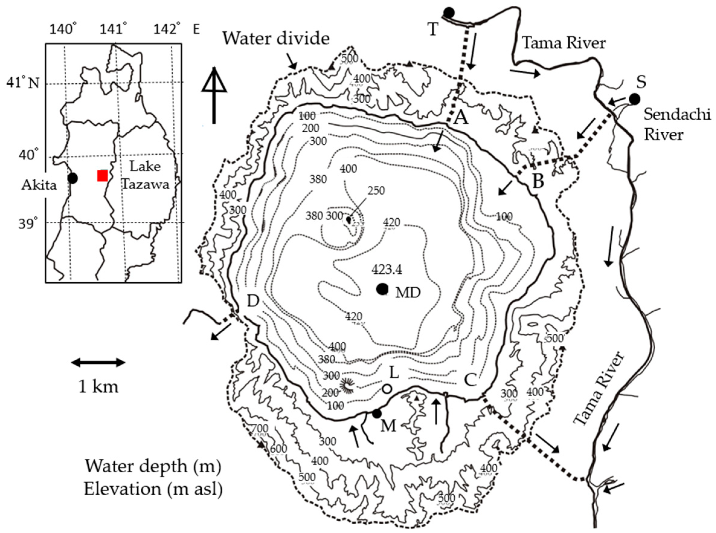
Lake Tazawa (39°43′30″ N, 140°39′41″ E), the deepest lake (maximum depth, 423 m) in Japan, is known as an acidic lake, since the Tama River water, including the Tamagawa hot spring of very high acidity at pH = 1.1–1.3, was drawn into the lake in 1940 [1,2] (Figure 1). The intake of the acidic river water drastically decreased the lake water’s pH from 6.5–6.7 before 1940 to 4.2–5.3 in 1948. Therefore, a land-locked type of sockeye salmon (alive at pH = 6.5–7.5), Oncorhynchus nerka kawamurae (local name, Kunimasu trout), was exterminated. The pH value increased up to 5.3–6.0 in 2019–2021 when a neutralization facility was established in the downstream of the Tamagawa hot spring site in April 1991. However, Kunimasu trout cannot yet inhabit the lake. At present, conduit B and conduit A are connected to the acidic Tama River (pH = 5.1–5.8) and the neutral Sendachi River (pH = 6.7–7.1), respectively, and power plants at the downstream end of conduit B and conduit C generate electric power levels of 7300 kW and 31,500 kW at maximum, respectively. The outflow at conduit D (previous natural outlet) is regulated to occur only in the irrigation season of May–August.
Meanwhile, Hayashi et al. [13] reported that the lake water temperature at a depth of 400 m of site MD increased at a rate of 0.05 °C per 10 years in August 1937–July 2017. The authors also indicated that the increasing rate increased to 0.013 °C/year in May 2015–July 2017. Such an abrupt increase in the hypolimnion’s temperature could not occur if the vertical water circulation in winter was strong enough to produce an isothermal condition through the continuous cooling at lake surface. Hence, the increasing rate suggests (1) that, as the cooling was weakened by global warming, the vertical water circulation in the lake did not occur in the whole layer, or (2) that the geothermal heat at the bottom was conserved by the incomplete water circulation [14]. With respect to Case 1, the annual lowest water temperature at the lake’s surface was recorded at ca. 2 °C in the 1910s [15], but around 4 °C in 2018 [2]. This suggests that vertical mixing in the lake changed in a dimictic to monomictic or oligomictic state.
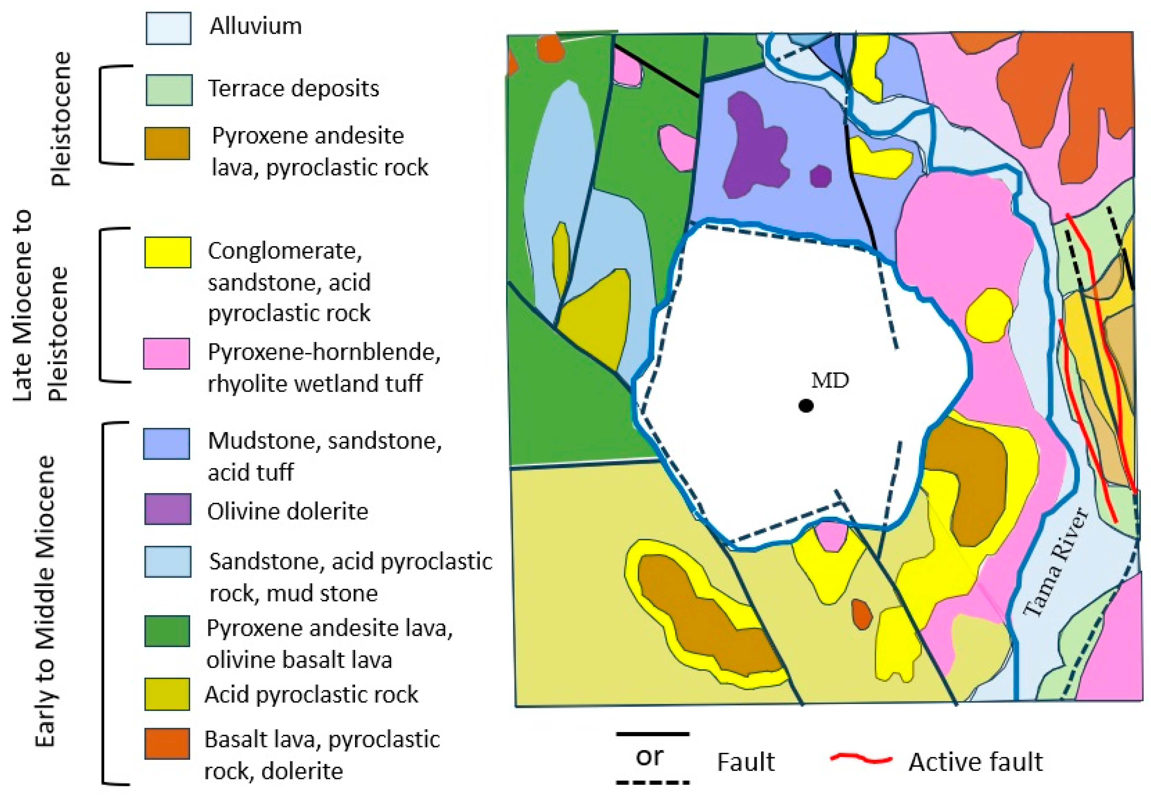
The geology and locations of faults or active faults in and around the lake are shown in Figure 2. The caldera of Lake Tazawa is inferred to have been formed 1.8–2 million years ago in the early Pleistocene by a catastrophic volcanic eruption [16]. There exist many faults and some active faults around the lake due to the tectonic movement. The lake is considered to have been built up through a series of volcanic events in the relatively old volcanic rock zone with the faults. It is thus noted that some of the faults remain on the bottom basin along the lake shore (thick dotted lines in Figure 2). The water depth of the bottom faults is about 100 m (Figure 1). The bottom faults could act as conduits of groundwater flowing into the lake, since the faults around the lake may possibly be permeable for precipitation [17].
3. Methods
In order to investigate a thermal system in Lake Tazawa, the heat budget of the lake was estimated. Then, the heat budget at the lake’s surface and the heat flux by river inflow and groundwater inflow were evaluated by estimating the hydrological budget of the lake [2].
3.1. Heat Budget of an Open Lake
The heat budget equation for an open lake (with an outflow river or an outlet) such as Lake Tazawa is given as follows:
where is the total heat storage change (W or J/s) of the lake; is the net radiative heat flux (W/m2) at the lake’s surface; and are the sensible and latent heat fluxes (W/m2) at the surface, respectively (negative for heat output); is the heat flux due to precipitation over the lake; is the heat flux due to the river; HG is the heat flux due to groundwater; HS is the geothermal heat flux at the lake’s bottom; and A0 is the lake’s water surface (m2).
The net radiative heat flux is composed of downward shortwave radiation , downward longwave radiation and upward longwave radiation as follows:
where α is the albedo of shortwave radiation for the water surface (here, assumed to be constant at 0.05). The upward longwave radiation is calculated by following the Stefan–Bolzman law for the surface water temperature (K), where the emissivity ε of the water is constant at 0.97. The downward longwave radiation was evaluated by considering the total effective water vapor content using the Stefan–Boltzmann law for air temperature Ta [19].
Sensible heat flux QH and latent heat flux QE were assessed by the following bulk transfer method:
where is the isobaric specific heat of air (J/kg/K); is the air density (kg/m3); λ is the latent heat of evaporation (J/kg); u is the wind speed (m/s); Ts and Ta are the surface water temperature and air temperature, respectively (°C); qs is the saturated specific humidity at the surface water temperature; qa is the specific humidity of the air; and CH and CE are dimensionless bulk transfer coefficients for sensible and latent heat fluxes, respectively (here, CH = CE = 0.0014 for the meteorology at 2 m above the lake’s surface).
The heat flux QP by rainfall over the lake is given in the following:
where is the water density (kg/m3) at Tw, Pr is the rainfall (m/s), cpw is the specific heat of water (J/kg/K), and Tw is the wet bulb temperature (°C). The Tw values were obtained using the dichotomy for the following psychrometer formula [19]:
where p is the air pressure (hPa) (p0 = 1013.2 hPa); ea and ew are the water vapor pressure (hPa) at Ta and the saturated water vapor pressure (hPa) at Tw, respectively; and B is the psychrometer constant (here, 0.667 hPa/K for the Assman ventilation psychrometer).
The heat flux by snowfall is as follows:
where is the ice density (kg/m3) at Ta; Pi is the snowfall (m/s) as ice at Ta; cpi is the specific heat of ice (J/kg/K); Tmelt is the melting temperature of ice (here, 273 K or 0 °C); and L is the latent heat of fusion (333.6 kJ/kg for ice at 0 °C). The precipitation during snowfall is generally evaluated by melting the snow over a tipping bucket raingauge. Hence, the snowfall at Ta was obtained by multiplying the precipitation at 0 °C during snowfall by the ratio of water density (999.868 kg/m3 at 0 °C) to ice density at Ta. Here, the snow temperature was assumed to be equal to the air temperature Ta. The precipitation at Ta ≤ 0.5 °C was supposed to be snowfall [19] on the assumption that, at 0.5 ≥ Ta > 0 °C, the snow temperature would be 0 °C. Then, the first term of the right side in Equation (7) would be zero.
The heat flux HR due to river inflow and outflow and the heat flux HG due to groundwater inflow and outflow are given as follows:
where Rin and Rout are the river inflow and outflow (m3/s), respectively; TRin and TRout are the water temperature of the inflowing and outflowing rivers, respectively; To is the water temperature averaged in the surface layer of the lake for the river inflow or outflow; TG0 is the water temperature of the layer receiving the groundwater inflow; TL is the representative lake water temperature; Gin and Gout are the groundwater inflow and outflow (m3/s), respectively; TGin and TGout are the temperature of inflowing groundwater and that of outflowing groundwater, respectively; and Ao is the lake’s surface area (m2). Here, it was assumed that the inflowing river water intruded into the surface layer only at depths of 0–10 m as density overflow [20]. Hence, considering each area from the bathymetric map (Figure 1), the volume-averaged water temperature at depths of 0.2–10 m was calculated as T0 in Equation (8). The water temperature at 0.2 m depth was then supposed to be equal to that at the lake’s surface.
Chikita et al. [21] adopted the local annual mean air temperature as TG0 in Equation (9) for the heat budget of a hydrothermal pond. This was based on the supposition that the inflow of shallow groundwater occurs in the unconfined aquifer around the pond with a water temperature equal to the annual mean air temperature [22,23]. However, in a deep lake such as Lake Tazawa, water depths for the occurrence of groundwater inflow are possibly limited to the bottom basin of 100 m or less in depth, since many fractures are distributed in the bedrock on the steep bottom slope at depths of 10–100 m [24]; also, the faults exist on the bottom basin at a depth of ca. 100 m along the lake shore (Figure 2). Hence, the volume-averaged water temperature at depths of 10–100 m is given as TG0 for the groundwater inflow in Equation (9).
For the representative temperature TL, the volume-averaged water temperature of the whole lake is given by the following equation:
where H is the water depth at the deepest point; Tz and Az are the water temperature and the area at a depth of z, respectively; and V is the lake’s volume. Here, H and V also vary temporally according to the temporal change in lake level. Equation (10) is based on the assumption that the water temperature at a certain depth is horizontally equal, i.e., exhibiting the thermal structure of a horizontal multi-layer in the lake. The supposition of TL for the groundwater outflow is due to the fact that it is unknown at which depth the groundwater outflow prevails. Consequently, the second term of the right side in each of Equations (8) and (9) was regarded to be almost zero, because TRout and TGout are likely to be equal to To and TL, respectively.
The geothermal heat flux Hs was estimated by the temporal change in vertical water temperature profiles at the deepest point during the thermal stratification [14]. The symbols in Equations (1)–(10) and their units are shown in Table 1.
Finally, the total heat storage change ΔG/Δt was numerically obtained by calculating each term of the right side in Equation (1). Meanwhile, ΔG/Δt could be evaluated directly by monitoring the water temperature at some depths between the lake’s surface and the bottom. Hence, it was possible to judge whether the heat budget estimate was reasonable or not through a comparison with the heat storage change from the direct measurement.
3.2. Field Observations
In order to evaluate each term of the heat budget Equation (1), the meteorology (solar radiation, air temperature Ta, relative humidity, rainfall, air pressure, and wind velocity), and lake water temperature at a depth of 0.2 m were measured at 1 h intervals at site M on the lake shore and at site L for 1 August 2020–9 May 2023, respectively (Figure 1). Temperature loggers, TidbiT v2 (Onset Computer, Incorp., Bourne, MA, USA; accuracy of ±0.2 °C), were used for the monitoring of the surface water temperature. Rainfall at site M was recorded from April to October, and rainfall or snowfall from November to March was estimated using high correlation (R2 = 0.869, p < 0.001) with the rainfall data of a weather station at Senboku City, 6.5 km southeast of Lake Tazawa. At Ta ≤ 0.5 °C at site M, the precipitation was assumed to be snowfall, and at Ta > 0.5 °C, to be rainfall. Here, the existence of sleet, i.e., the mixture of snow flakes and raindrops, was neglected. The climatological effect on the lake was explored using the 1977–2023 data from the weather station of Senboku City.
At site L, the water temperature at a depth of 0.2 m was measured as the lake surface temperature to calculate the sensible and latent heat fluxes QH and QE via coupling with the meteorology, and the difference between the air pressure at site M and the water pressure at the bottom of site L allowed us to calculate the water depth to obtain the temporal variations in lake level. The lake surface area, which changed with the lake level was obtained using bathymetry with 1 m depth contours (Figure 1) [2]. Inflow data at the conduits A and B, connected to the Tama River and the Sendachi River, respectively, were supplied by the Tohoku Electric Power Co., Ltd. (Sendai, Japan) (Figure 1). The data supply was carried out every fiscal year of 1 April 2020–31 March 2023. Temperature loggers, recorded at 1 h intervals, were fixed on the riverbank at sites T and S at 0.66 km and 0.2 km upstream of the entrances of conduits A and B, respectively.
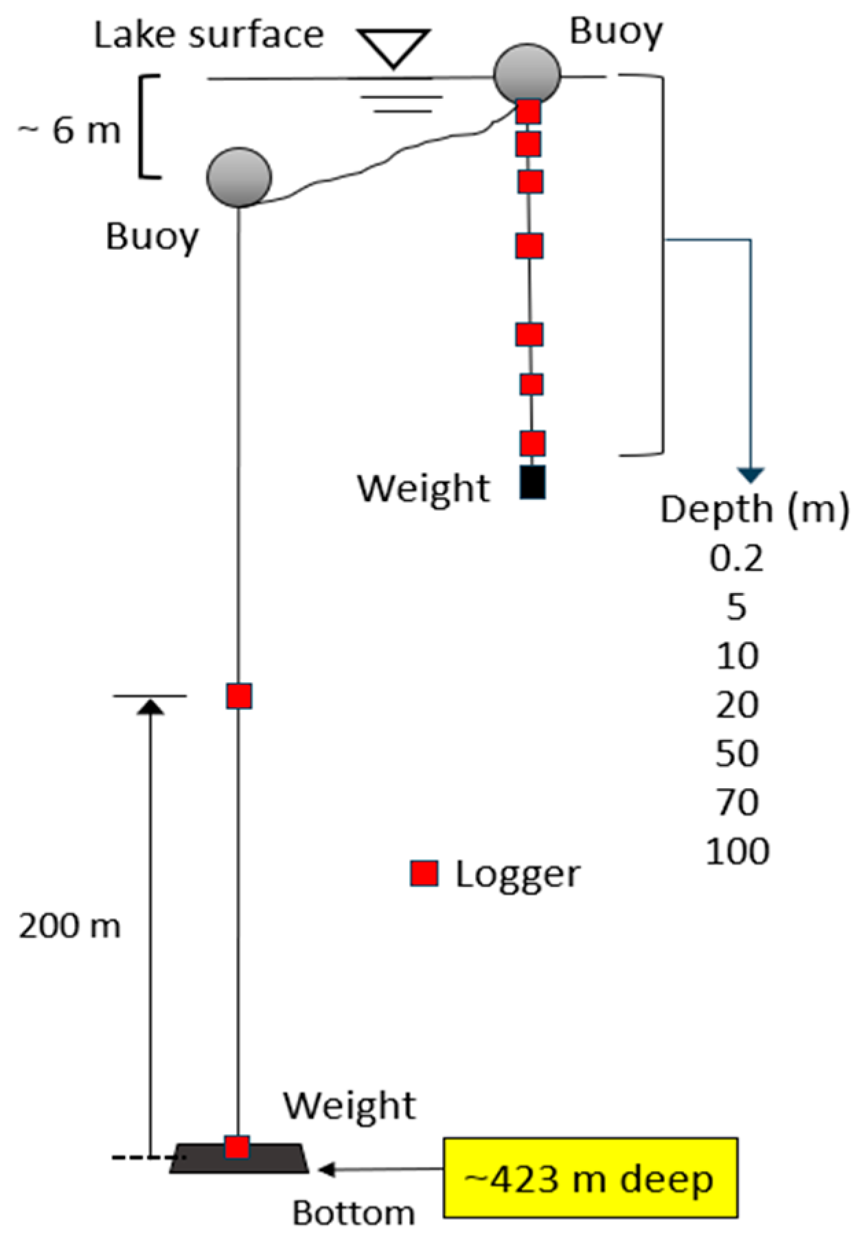
Meanwhile, the lake water temperature was recorded every 1 h at depths of 0.2 m, 5 m, 10 m, 20 m, 50 m, 70 m, 100 m, and 200 m above the bottom, and at the bottom of site MD by setting a mooring system of temperature loggers (Figure 3).
At a depth of 0.2 m and the bottom of the lake, temperature loggers with high accuracy of ±0.01 °C and resolution of 0.001 °C (model DEFI2-T, JFE-Advantech, Co., Ltd., Nishinomiya, Japan: Available online: https://www.jfe-advantech.co.jp/products/ocean-defi2.html, accessed on 12 October 2023) were fixed to judge the downward degree of vertical water circulation in the water. At the other depths, the temperature loggers, TidbiT v2, were fixed.
Water temperature, electric conductivity at 25 °C (EC25), and dissolved oxygen (DO) were vertically measured at a 0.1 m pitch by lowering a profiler onto a boat (accuracies of ±0.01 °C, ±0.5 mS/m and ±0.4 mg/L, respectively; model ASTD, JFE-Advantech, Co., Ltd., Japan: Available online: https://www.jfe-advantech.co.jp/products/ocean-rinko.html, accessed on 13 October 2023). The measurement with the ASTD profiler took about 40 min for a single point. Using the bathymetric map of the lake (Figure 1), the hourly heat storage Ghl (J) of the lake was calculated from the hourly temperature of the loggers. The Ghl values were calibrated using the correspondent heat storage Gp from the profiler, since there was a linear relationship between Ghl and Gp with a high correlation of R2 = 0.978 (p < 0.01). Using the calibrated Ghl, the heat storage change (W) in the lake was calculated as a daily mean, which was compared with the ΔG/Δt values from the heat budget estimate made using Equation (1).
3.3. Data Analysis
The hourly data of meteorology at site M; water level at site L; and water temperature at sites T, S, and MD were processed as daily mean time series to estimate the heat budget and heat storage change of the lake, since the inflow at the conduits of A, B, and C was supplied as daily means by the Tohoku Electric Power Co., Ltd. Thus, each heat flux or heat storage change in Equation (1) was calculated as a daily mean. Relations between the lake heat storage or volume-averaged water temperature calculated by the loggers’ data and that acquired by the vertical temperature profiles from the profiler were explored using the linear regression model, where the R2 (coefficient of determination) and p-value were obtained together with the regression equation. Daily mean time series of the heat storage change calculated were smoothed into the 10-day average time series, which were also applied to the linear regression model to obtain the RMSE and 95% confidence interval, as well as to perform hypothesis testing for the regression coefficients, assuming that the error had a normal distribution. The 3-month moving average time series were also obtained in order to reveal the seasonal variation in heat storage change.
4. Results
4.1. Heat Budget at Lake Surface
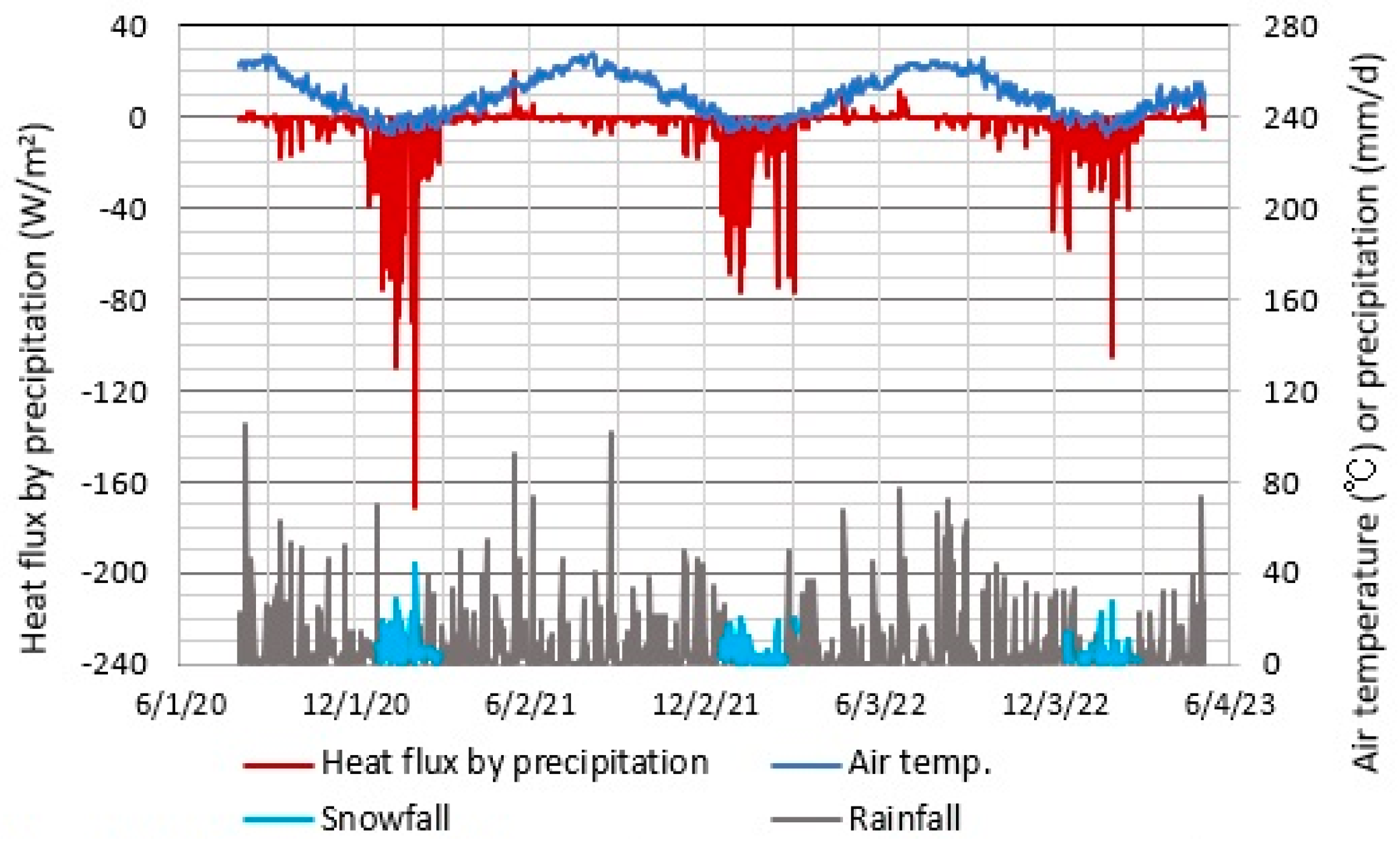
Temporal variations in the daily mean air temperature, diurnal precipitation, and daily mean heat flux at the lake’s surface with precipitation are shown in Figure 4. The precipitation was separated at Ta = 0.5 °C into rainfall and snowfall. With the rainfall, the heat flux by precipitation varied in a range of −20–20 W/m2, but with the snowfall, the heat flux reached −171 W/m2 on 2 February 2021, when the precipitation was recorded at 45 mm/d. Thus, the cooling at the surface due to snowfall is likely considerable.
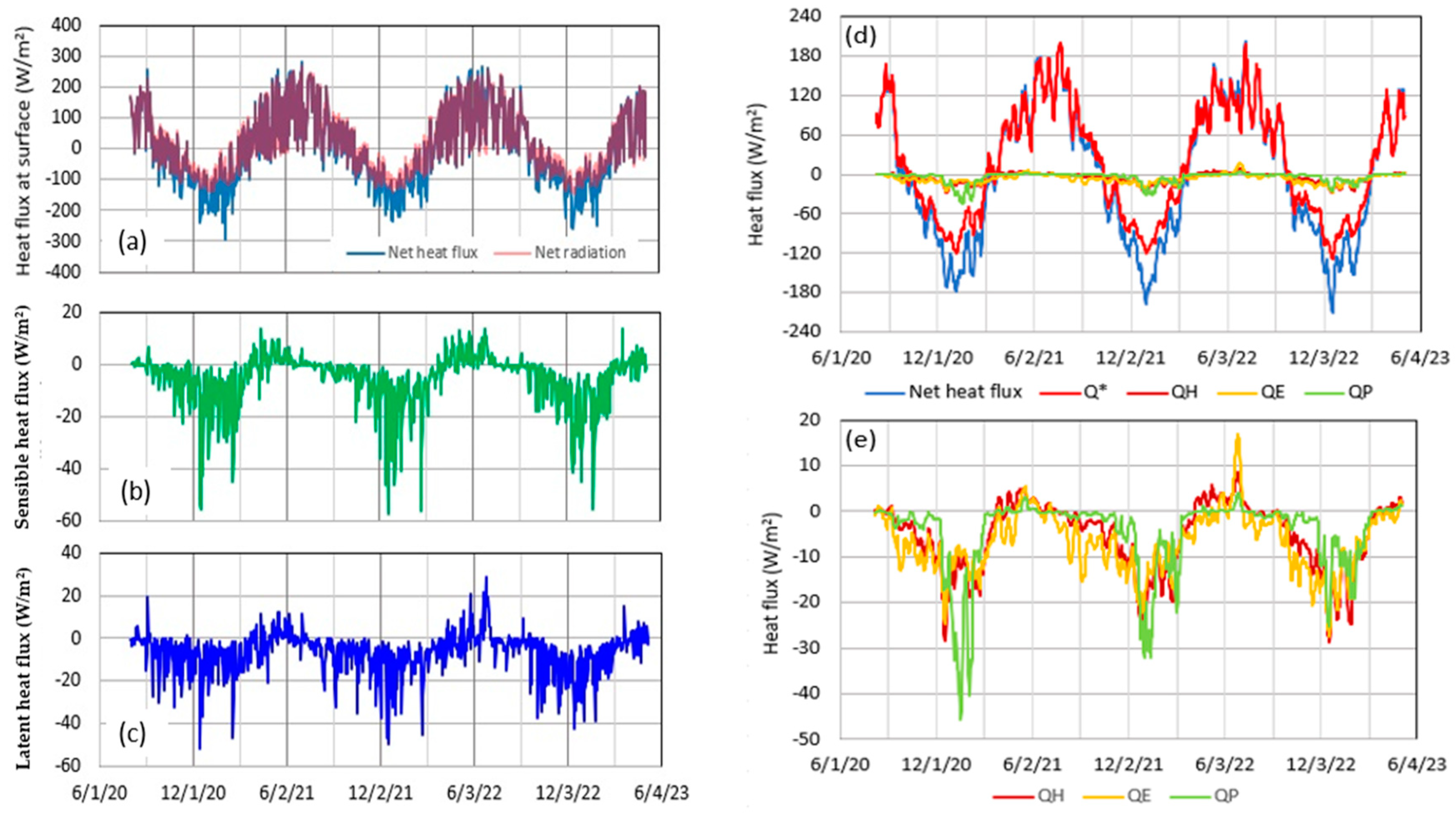
In order to clarify the contribution of Q*, QH, QE, and QP on the right side of Equation (1) to heating or cooling at the lake’s surface, their values, as calculated by Equations (2)–(6), were compared with their sum, i.e., the net heat flux (Figure 5a–c). In the rainfall season, the net heat flux was comparable in magnitude to the net radiation Q*, but in the snowfall season (December–March), the net heat flux consisted of 50% Q* and 50% (QH + QE). In particular, the heavy snowfall on 2 February 2021 produced a heat flux in magnitude at 58.4% of the net heat flux (−293.1 W/m2). The Q*, QH, and QE values were then −89.2, −17.4, and −15.6 W/m2, respectively, thus occupying 30.4, 5.9, and 5.3% of the neat heat flux in magnitude, respectively.
The time series of 10-day moving averages for the net heat flux, Q*, QH, QE, and QP are totally described in Figure 5d, and those for QH, QE, and QP are enlarged in Figure 5e. It can be seen that the contributions of QH, QE, and QP to the net heat flux become relatively large in December–February. In the cooling periods of negative net heat flux recorded continuously for two days or more, Q*, QH, QE, and QP occupied in magnitude 62.7%, 12.3%, 12.6%, and 12.4% for 1 October 2020–22 March 2021; 64.1%, 12.7%, 12.4%, and 10.8% for 12 October 2021–19 March 2022; and 65.6%, 12.7%, 14.1%, and 7.6% for 22 September 2022–3 March 2023, respectively. Thus, it was found that QP cannot be neglected in the cooling periods.
The Q*, QH, QE, and QP values and their percentages in magnitude were averaged for the snowfall periods of December 2020–February 2021 (Table 2). The Q* values were negative at any time point in the snowfall periods, reflecting the larger magnitude of upward longwave radiation than the downward longwave radiation plus the net solar radiation in Equation (2). As averages over the snowfall periods, the QP value and its percentage in magnitude were −30.9 W/m2 and 19.2%, respectively. This clearly indicates that the heat loss due to snowfall is effective for cooling at the lake’s surface.
Compared with the QP value (−0.6 W/m2) averaged over the rainfall periods and that (−1.2 W/m2) over rainfall days in February–December 2021, the mean QP value (−3.8 W/m2) on the rainfall days in the snowfall period was more effective for cooling at the lake’s surface (Table 2). It can be seen that, on the non-rainfall days in the rainfall period, the net radiation dominated the heating at the lake’s surface.
4.2. Heat Flux by River and Groundwater
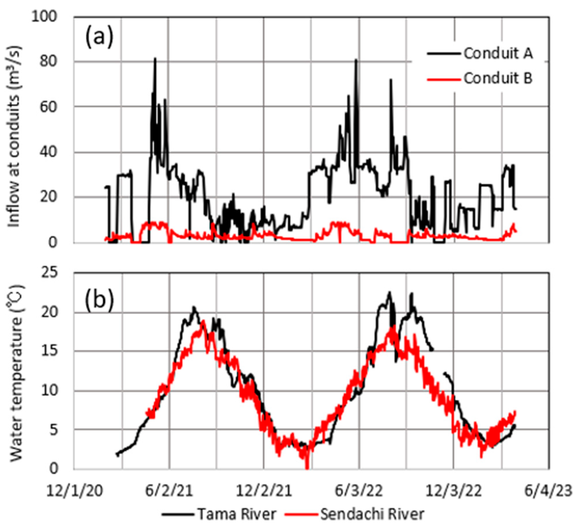
Temporal variations in the daily mean river inflow at conduits A and B and the daily mean river water temperature at sites T and S are shown in Figure 6. For the period of 1 February 2021–31 March 2023, the water temperature varied seasonally, while the inflow at the conduits varied under the artificial control following the snowmelt in March–April and the relatively large water demand for the paddy fields in the irrigation season of May–August. For the maintenance of the power plants at the conduits A and B, zero inflow occurred outside of the irrigation season (Figure 6a). The inflows averaged for the two years of 1 February 2021–31 January 2023 were 20.1 m3/s at conduit A and 3.0 m3/s at conduit B. Thus, similarly to the heat flux by river inflow, that by the Tama River could be dominant because of the similar magnitude of water temperature of the two rivers (Figure 6b).
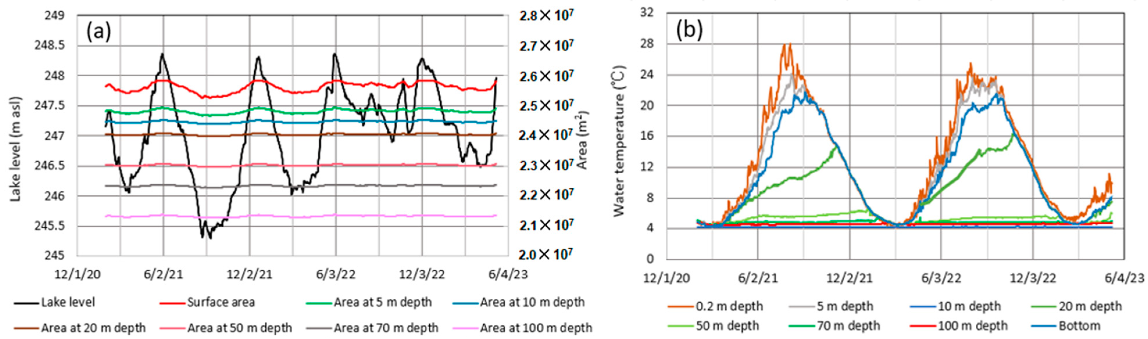
In order to calculate the heat flux according to river inflow in Equation (8), the volume-averaged water temperature To at depths of 0–10 m was numerically obtained by applying water temperature at depths of 0.2 m, 5 m, and 10 m (Figure 7b) and the lake basin shape (Figure 1) to Equation (10). Then, the temporal variation in lake level, surface area, or each area at 5 m depth and 10 m depth from the basin shape was taken into account (Figure 7a). Here, the water temperature at a depth of 0.2 m was supposed to be equal to that at the lake’s surface. Following the total river inflow in Figure 6a, the lake level varied with the maximum amplitude of 3.06 m in 2021, when the surface area ranged between 2.527 × 10⁷ and 2.583 × 10⁷ m2.
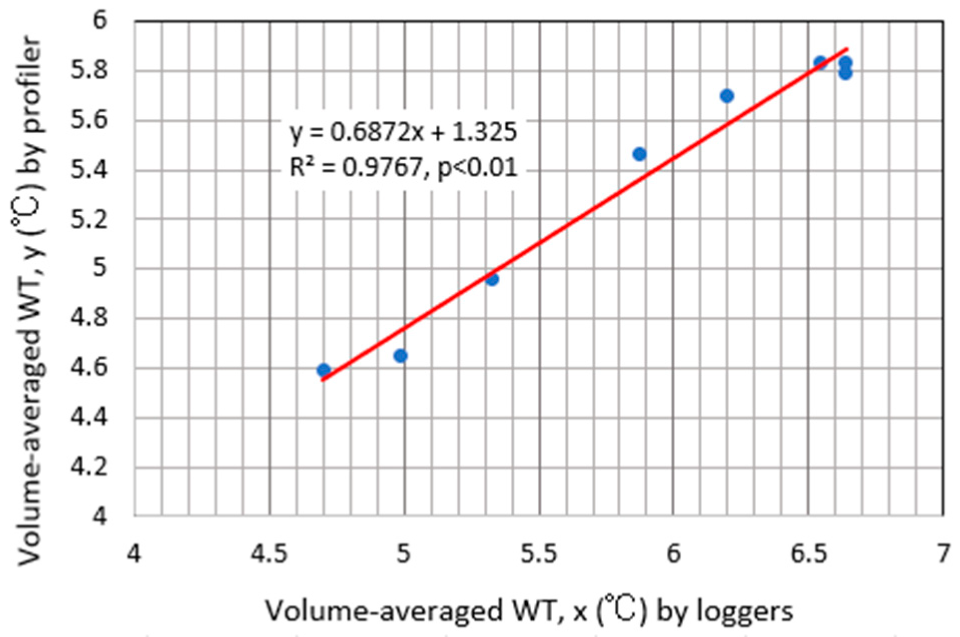
All the data on the water temperature and area in Figure 7 were utilized to calculate the volume-averaged lake temperature TL in Equation (10). Then, the area at the bottom was regarded as a constant at 1.007 × 10⁶ m2. Also, the volume-averaged water temperature from the time series of water temperature in Figure 7b was calibrated by that from the corresponding profiles at 0.1 m pitch (Figure 8). In the calculation of TL from the profiles, considering the significant seasonal variation in water temperature at depths of 100 m or less and the basin shape in Figure 1, the heat storage of the lake was calculated every 5 m depth at depths of 100 m or less. At depths of more than 100 m, the area was obtained every 100 m of depth at depths of 100–300 m, every 10 m of depth at depths of 380–410 m, and at the bottom (412.2–422.6 m in depth). The area at a certain depth of 100 m or less was then obtained by partitioning each 10 m contour into two equal parts on the bathymetric map with 10 m depth intervals.
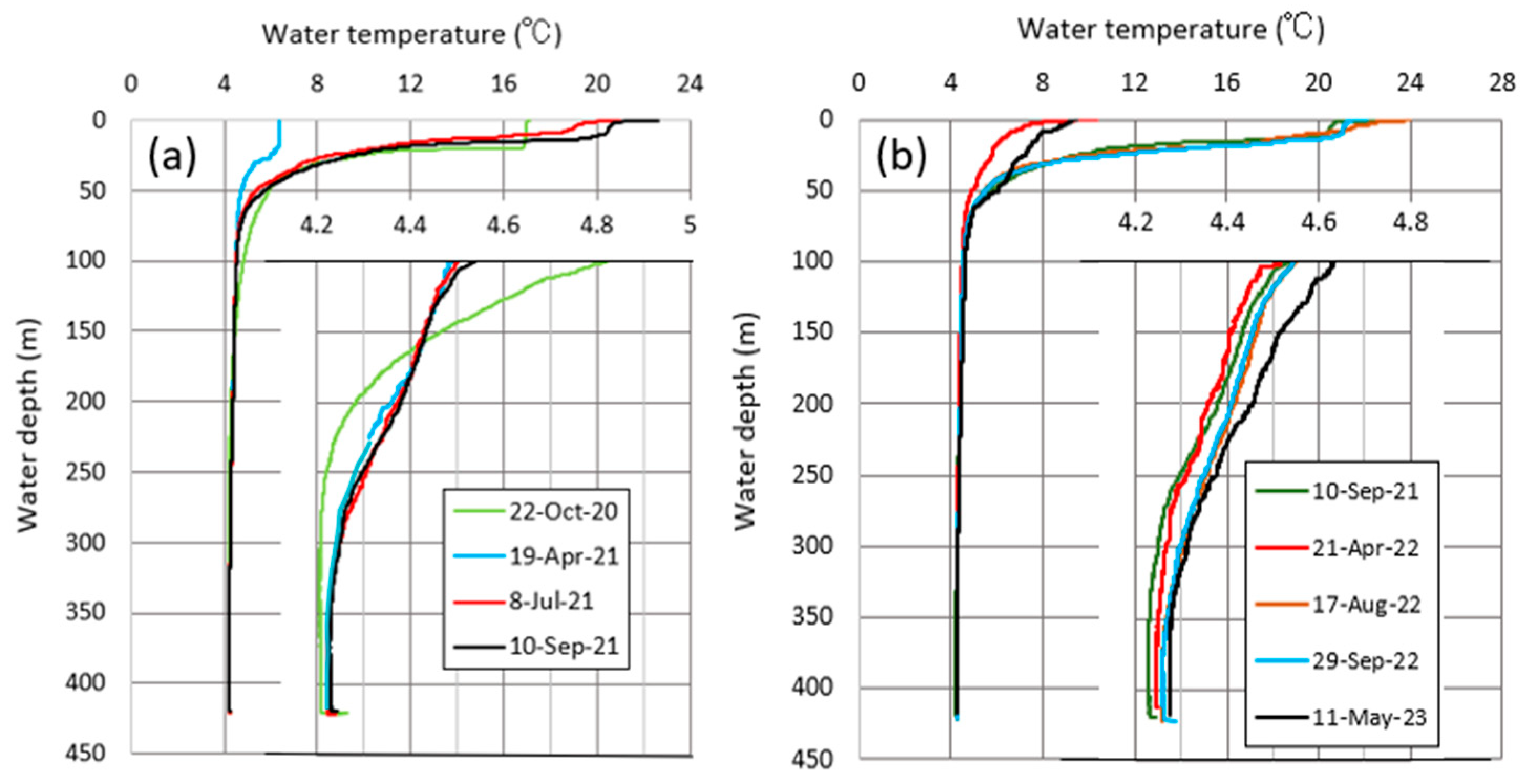
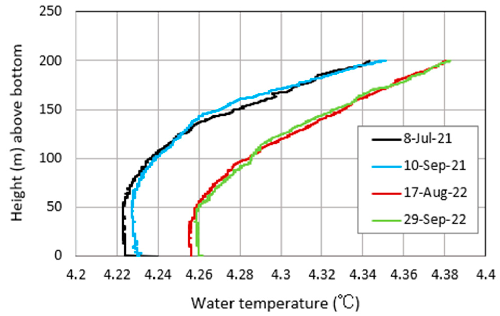
Meanwhile, at depths of 100 m or more, the water temperature also increased gradually (see that inserted diagrams in Figure 8), especially before and after the winters, as shown by the 22 October 2020 and 19 April 2021 profiles, the 10 September 2021 and 21 April 2022 profiles, and the 29 September 2022 and 11 May 2023 profiles. During the thermal stratification in summer to autumn, such an increase was slight. Hence, the vertical circulation in winter is likely not to be strong enough to make the water temperature vertically uniform in the whole layer. Such an increase in water temperature in the short term, i.e., 2 years or slightly more, is probably not related to global warming but to the geothermal heat flux Hs at the bottom in Equation (1), since the effect of global warming can be found by investigating the trend in air temperature from decadal or larger time-scale data.
Consequently, there was a linear relationship with the high correlation of R2 = 0.977 (p < 0.01) between the volume-averaged temperature from the loggers and that from the profiles (Figure 9). Of the eight plots in Figure 9, the two nearest plots on the right were produced from two measurements on 17 August 2022 (Figure 8). In Figure 9, it is clear that the TL values from the loggers were overestimated by 0.1–0.8 °C.
The groundwater inflow was supposed to be constant at 6.01 m3/s, according to the water budget estimate for Lake Tazawa by Chikita et al. [2], since there are no data on the heat difference between the lake level and groundwater table around the lake shore. However, there was a small difference in annual precipitation in 2020–2023, with a mean of 2374 mm and a standard deviation of 163 mm. According to Kobayashi [22] and Arai [23], the temperature, TGin, of inflowing groundwater was assumed to be constant at 10.5 °C, which is equal to the annual mean air temperature at site M for 1 February 2021–31 January 2023. Here, for the water temperature, TG0, in Equation (9), the volume-averaged temperature at depths of 10–100 m was given because of the presence of many fractures at depths of 10–100 m [24] and fractures at ca. 100 m depth along the lake shore (Figure 2), which could act as conduits of groundwater flow. Consequently, the heat flux by groundwater inflow exhibited annual cycles, with maximums (6.0–6.2 W/m2) in late Februaly or early March and minimuns (1.9–2.0 W/m2) in August or September as the heating occurred. The annual cycles reflect the seasonal variations in the water temperature at depths of 10–100 m (Figure 10a).
The heat fluxes due to the inflow of the Tama River (conduit A) and the Sendachi River (conduit B) are also shown in Figure 10a. The heat flux due to river inflow exerts a cooling effect on the lake in most of the period, sporadically exhibiting sharp, negative peaks.The sharp peaks are due to relatively large discharge with decreased water temperature in the Tama River, which is supplied by the upstream Yoroibata Reservoir (Figure 6). Compared with the QH, QE, and QP values, the heat flux by river inflow makes a minor contribution to the cooling or heating of the lake in the rainfall period of March–November, but its contribution is more negligible in the snowfall period of December–February (Figure 6 and Figure 10b).
4.3. Geothermal Heat Flux
The geothermal heat flux HS in Equation (1) was estimated by calculating an increasing rate of water temperature in the bottom layer [14]. Actually, for the vertical profiles in Figure 7, the bottom layer of 0–118.4 m and the layer 0–101.5 m above the bottom consistently increased the water temperature in the thermal stratification periods of 8 July–10 September 2021 and 17 August–29 September 2022, respectively (Figure 11). Here, considering the lake basin shape in Figure 1, the total heat storage was calculated for the layers of 0–118.4 m in 2021 and 0–101.5 m in 2022, and then the heat storage changes in 2021 and 2022 were obtained as Hs in Equation (1). As a result, Hs = 0.23 W/m2 and 0.25 W/m2 were acquired for 2021 and 2022, respectively, which are near the 0.27 W/m2 value found by Boehrer et al. [15]. Thus, the geothermal heat flux appears to be negligibly small compared with the heat flux due to groundwater inflow at 1.9–6.2 W/m2 and the other heat fluxes (Figure 5 and Figure 10). There exists a small volcanic effect on the heat budget of the lake, although an active volcano, Mt. Komagatake, is located at 12.3 km east-northeast of the lake.
Meanwhile, the geothermal heat could be conserved at the bottom if the lower limit of vertical water circulation were far from the bottom, and thus, no remarkable upward thermal diffusion would occur. The consistent increase in the bottom layer (inserted graphs in Figure 8), thus, possibly reflects the geothermal heat storage in the lower layer.
5. Discussion
5.1. Comparison of Heat Storage Change
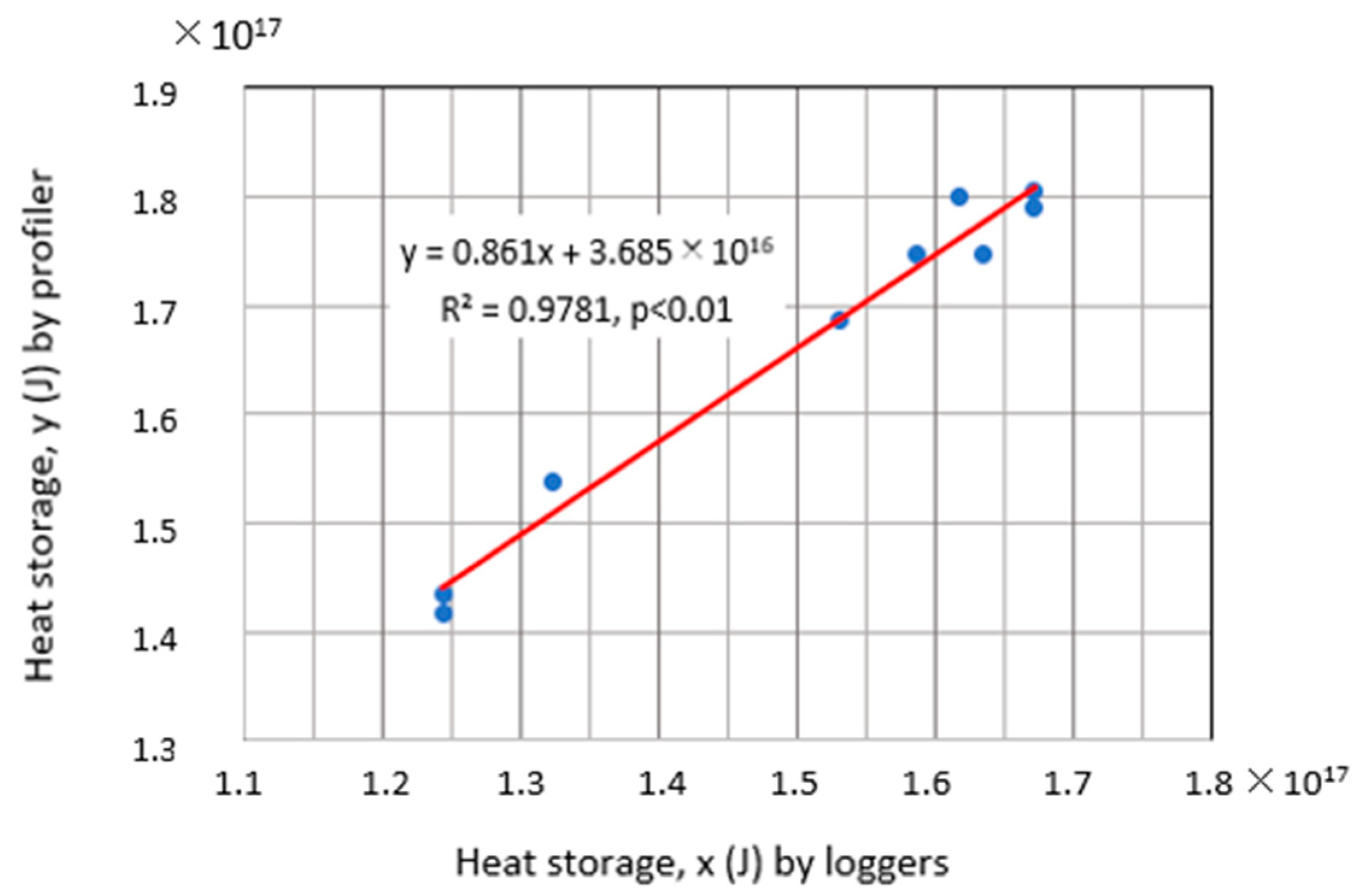
For Equation (1), the left side and the right side were evaluated and compared using the heat storage change from the temperature monitoring and the heat budget estimate, respectively. Then, the heat storage G (J) from the temperature loggers at depths of 0.2 m, 5 m, 10 m, 20 m, 50 m, 70 m, and 100 m and at the bottom of site MD was calibrated by that from the corresponding vertical temperature profiles in Figure 7 using the high correlation (R2 = 0.978, p < 0.01) between the two heat storages (Figure 12). Then, the lake basin shape in Figure 1 was considered, as was the case in the calculation of volume-averaged water temperature TL. In contrast to the TL values (Figure 8), the heat storage from the loggers tends to be underestimated. This is because the lake basin volume in the calculation from the profiles is larger than that in the calculation from the loggers. Here, the former volume is nearer to the actual lake volume.
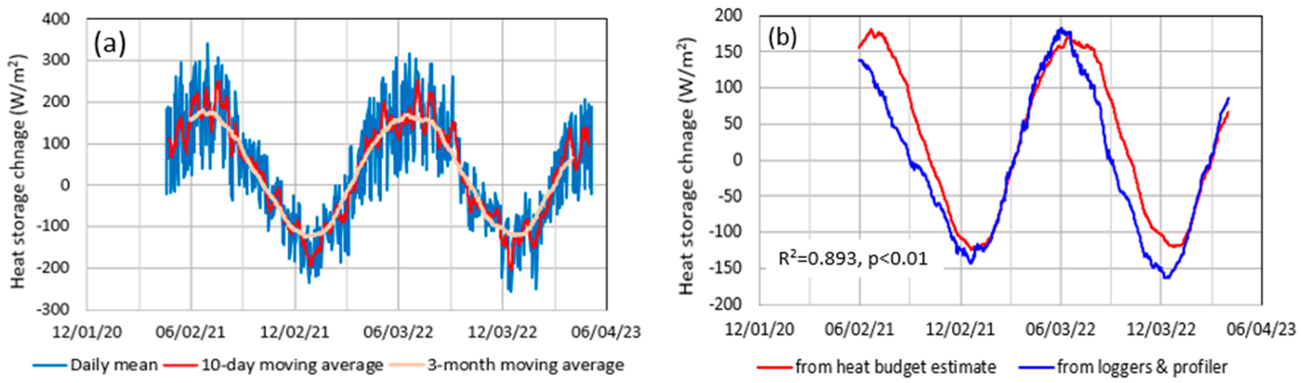
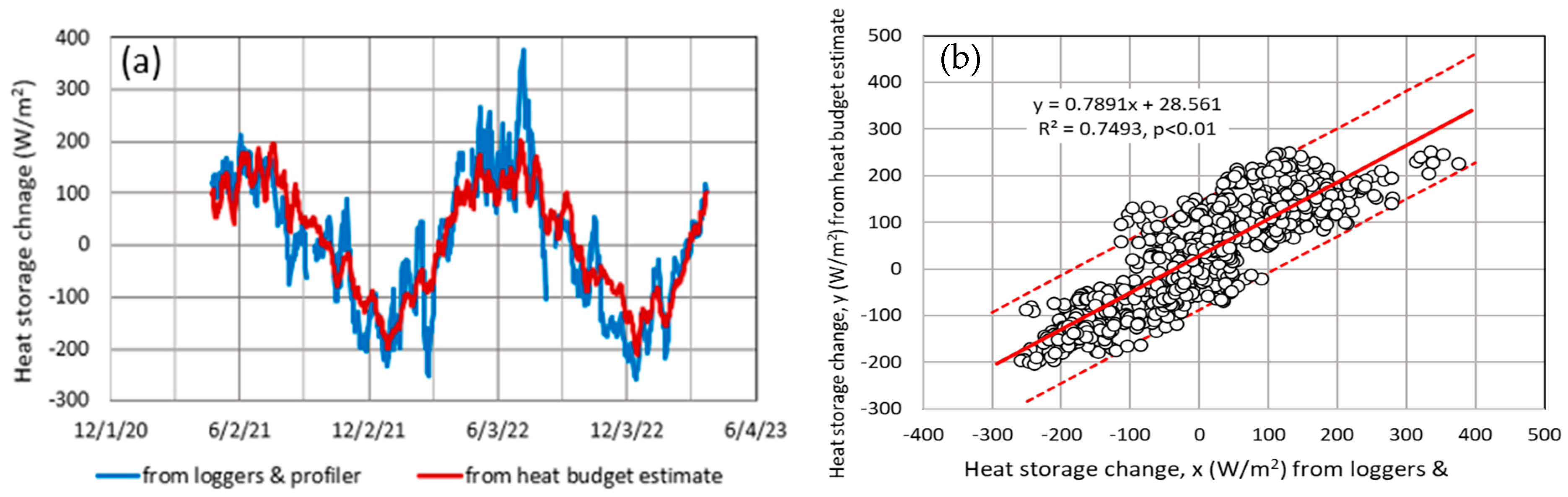
The heat storage change from the heat budget estimate is shown as a daily mean time series of 20 April 2021–31 March 2023, as well as their 10-day and 3-month moving averages (Figure 13a). The seasonal variation in the heat storage change is clearly depicted by the 3-month moving average. Focusing on the 3-month moving average, the heat storage change annually varied between 180 W/m2 in late-June 2021 and −124 W/m2 in late December 2021 and between 163 W/m2 in early July 2022 and −120 W/m2 in late December 2022. The correlation between the two 3-month moving average time series was very high at R2 = 0.893 (p < 0.01) (Figure 13b). The fitting between the two was better in the heating season, while in the cooling season, the heat storage change from the heat budget estimate tended to be overestimated.
Using the regression equation for the 10-day moving average time series in Figure 14b, the root mean square error (RMSE) between the two was 58.6 W/m2 over the periods of 24 April 2021–26 March 2023 (Figure 14a). In the period of May–July 2022, the assumption that the water temperature was horizontally equal at a certain depth (i.e., the thermal structure of a horizontal multi-layer) likely did not hold. One of reasons for this is probably that the consistently large inflow from the Tama River (Figure 6a) produced thermal heterogeneity in the surface layer as the cooling agent offshore from the outlet of conduit A (Figure 1). Actually, on 13 August 2022, the heat storage change from the loggers’ data greatly decreased (Figure 14a). This may have been caused by the relatively large negative heat flux from the Tama River on 9–18 August (Figure 10a).
The correlation between the two heat storage changes in Figure 14a is shown in Figure 14b, with a 95% confidence interval. The heating and cooling stages separated by the boundaries of December–January and June–July exhibited high correlations at R2 = 0.749. In fact, almost all the plots were located in the 95% confidence interval. The heat storage change from the heat budget estimate caused the difference by providing overestimated values in the early cooling stage and underestimated ones in the late heating stage (Figure 14a). In the winter, in December–February, all the terms, i.e., , , , and at the lake’s surface in Equation (1), should be taken into account to estimate the heat storage change. In the cooling stage, in addition to , , and , the heat flux due to the Tama River could sporadically affect the heat storage change (Figure 10).
5.2. Lower Limit of Vertical Water Circulation
As shown in Figure 7b, the water temperature at a depth of 0.2 m was very close to the bottom temperature of 4.21–4.27 °C for the periods of mid-February–early March. Hence, based on a comparison between the vertical change in the dissolved oxygen (DO) and the lake water temperatures at a depth of 0.2 m and at the bottom water, it was judged at what depth the vertical circulation of the lake water occurred.
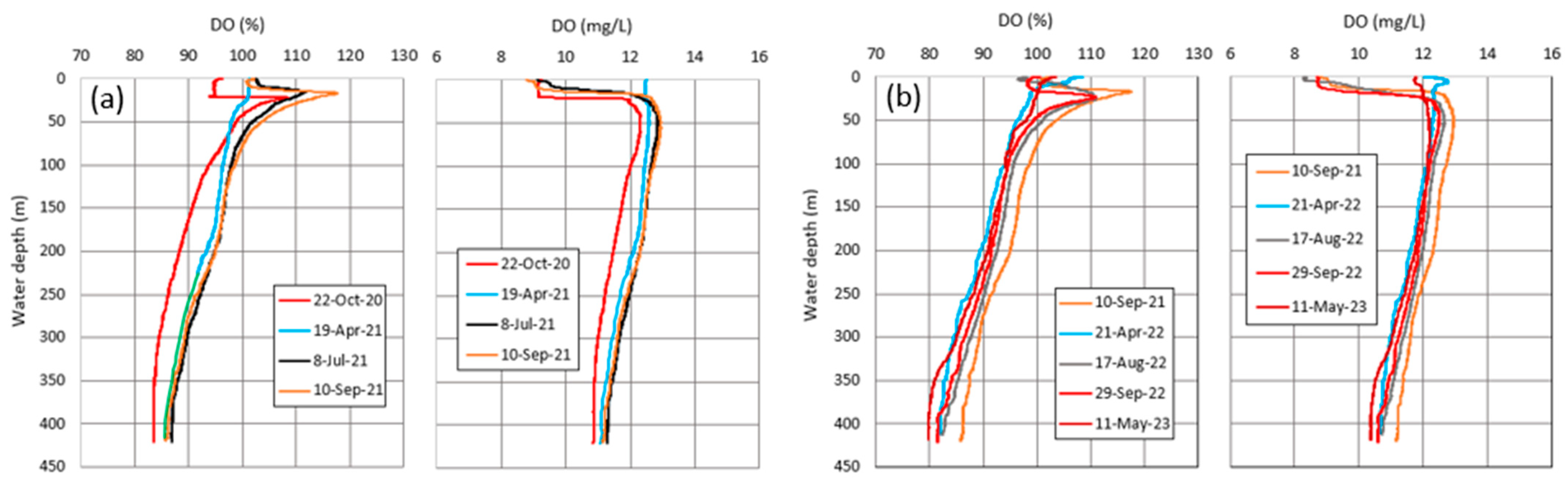
Vertical distributions of DO in % and mg/L, corresponding to those of the water temperature in Figure 8, are shown in Figure 15. As shown in Figure 8, the water temperature in the thermally stratified season changed little temporally at depths of more than 100 m. The DO at depths of more than 100 m could thus be supplied only by the vertical water circulation in winter, when the water temperature was vertically almost uniform around 4.2 °C.
In July–October, with the clear thermocline in Figure 8, DO peaks with oversaturation near the depth of the thermocline probably occurred due to the photosynthesis of phytoplankton, but then maintained more than 80%, even at depths of more than 100 m. The latter suggests that the DO loss was small due to the decomposition of less organic matter in the acid lake (pH, 5.3–6.0) [2]. The DO at a depth of more than 100 m could thus be redistributed only by vertical water circulation into the deeper zone. As an average, over depths of more than 100 m, the DO increased at a rate of 0.0026 mg/L/day in 22 October 2020–19 April 2021 (179 days), but decreased at a rate of 0.0033 mg/L/day in 10 September 2021–21 April 2022 (223 days) and at a rate of 0.00071 mg/L/day in 29 September 2022–11 May 2023 (224 days).
Meanwhile, in spring to autumn, with no vertical water circulation at depths of more than 100 m, the DO increased at an average rate of 0.0011 mg/L/d in 19 April–10 September 2021 (144 days) and in 21 April–29 September 2022 (161 days). Hence, the increasing rate of 0.0011 mg/L/d was regarded as a threshold when, at the lower value, the vertical water circulation did not occur at a depth of more than 100 m. The increasing rate of 0.0026 mg/L/day, averaged over 22 October 2020–19 April 2021, thus suggests that the vertical water circulation reached the bottom in February–March 2021 (Figure 7b). On the contrary, the rate of −0.0033 mg/L/day for 10 September 2021–21 April 2022 and the rate of −0.00071 mg/L/day for 29 September 2022–11 May 2023 suggest that the vertical circulation did not reach the bottom. The large DO loss in September 2021–April 2022 especially implies the occurrence of vertical circulation limited to the surface layer above the thermocline (see the 10 September 2021 and 21 April 2022 profiles in Figure 8 and Figure 15b). In September 2022–May 2023, with the decreasing rate of 0.00071 mg/L/day, vertical circulation probably did not occur in the deeper zone, since the rate was close to 0.0011 mg/L/day in spring to autumn. Actually, a comparison between the 29 September 2022 and the 11 May 2023 profiles in Figure 15b allows us to find that, at depths of more than 200 m, the DO decreased, which was probably because no vertical circulation occurred in the deeper zone.
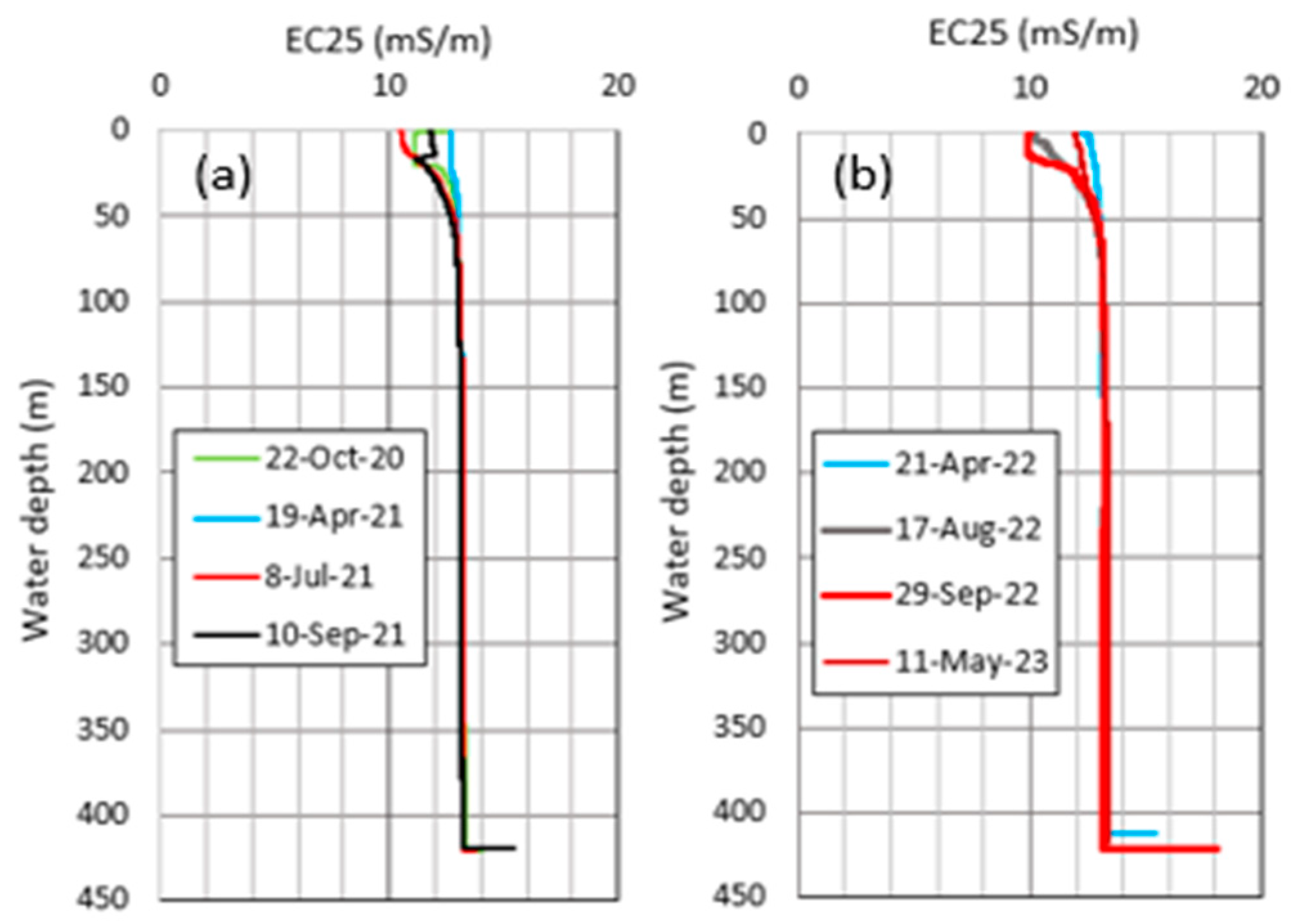
Here, in order to investigate the vertical water circulation between the surface and the bottom of the lake, the potential temperature was calculated for the water at the bottom. This was because the water density is a function of water temperature, pressure, and salinity. The profiling at site MD in the lake showed a salinity level of 0.040–0.054‰, corresponding to an EC25 (electric conductivity at 25 °C) of 10.0–13.4 mS/m (Figure 16). Here, a relation between EC25 (x) in mS/m and salinity (y) in ‰ was given by y = 0.00428x − 0.00293 (R2 = 0.999, p < 0.001) for the profiler. Hence, according to Jackett et al. [25], the potential temperature for the bottom water at 4.20–4.30 °C (Figure 8) and 412–413 dbar was evaluated at 4.194–4.293 °C at the water’s surface. The water temperature recorded at the bottom can thus be compared directly with the temperature at a depth of 0.2 m because of the slight difference (0.006–0.007 °C) within the accuracy of ±0.01 °C (resolution, 0.001 °C) for the loggers used.
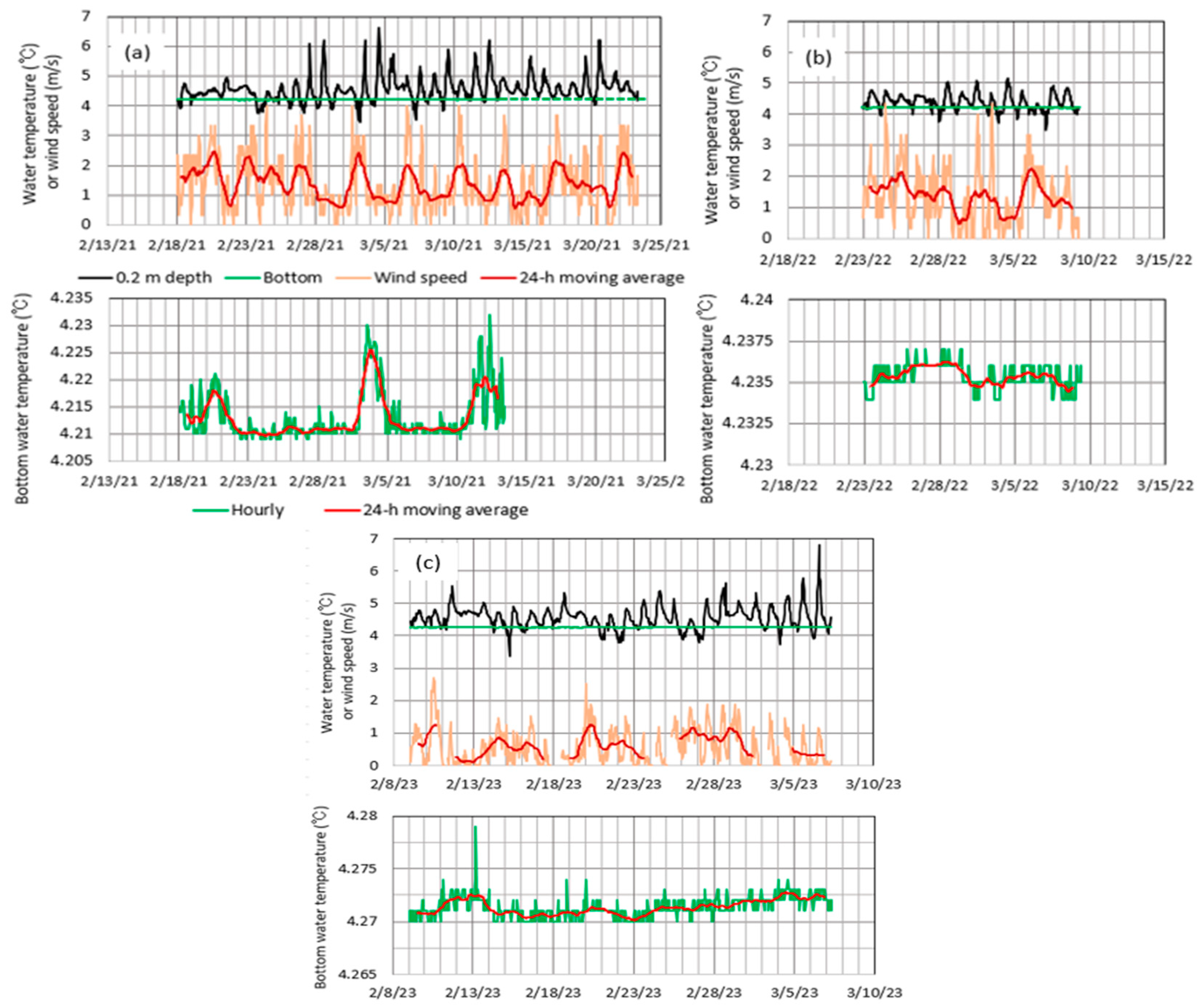
Here, relations between the temperatures at a depth of 0.2 m and at the bottom and the wind speed in the three winters of 2021–2023 are detailed in Figure 17. The addition of the wind speed data was due to its significant effect on the vertical mixing under the condition of no thermal stratification [9,10]. Farmer and Carmack [10] proposed a mixing layer model where both nonlinearity and pressure dependence were considered in the equation of state. As the expansion coefficient of freshwater was very small near a water temperature of 4 °C, the pressure effect dominated the stability. When a given water temperature at constant pressure is equal to the temperature with maximum density, the water depth at the given temperature becomes a boundary between forced and free convections. Below the water depth, the water is gravitationally unstable. As far as such a boundary exists, conditional instability, where initially stable water moving downward produces gravitational instability, occurs. The conditional instability continues as far as wind produces water with maximum density. Thus, if the wind is strong under the conditional instability, the downward movement of water could be promoted. Hence, referring to a water temperature of 4 °C, a comparison between the temperature at a depth of 0.2 m and at the bottom at a certain wind speed is necessary to judge if or not the vertical water circulation reached the bottom.
In Figure 17, the hourly or 24 h moving average variations in the surface and bottom water temperatures and wind speed are drawn only for the periods when the temperature at a depth of 0.2 m was less than the temperature at the bottom. Below the bottom water temperature, the surface water could sink into the deeper layer by producing relatively heavy water from the mixture with the water below. The data failure for the bottom temperature occurred for the period of 1100 h, 13 March–1000 h, 23 March 2021 (Figure 17a), when the values were extrapolated at 4.125 (green dotted line).
Of all three of the periods in 2021–2023, including the hours when the temperature at a 0.2 m depth was less than the bottom temperature, the period in 2021 was longest at 200 h, 18 February–700 h, 23 March (in total, 118 h for 33.21 days) (Figure 17a), while the periods in 2022 and 2023 were 0 h, 23 February–800 h, 9 March (in total, 96 h for 14.33 days) (Figure 17b) and 300 h, 9 February–500 h, 7 March (in total, 110 h for 26.08 days) (Figure 17c), respectively. The temporal variation in bottom temperature above the accuracy of the logger then occurred only for the three time periods of (1) 300 h–2200 h, 20 February; (2) 2100 h, 2 March–1900 h, 4 March; and (3) 400 h, 11 March–600 h, 13 March (Figure 17a) in 2021. Compared with the hourly 0.2 m temperature and wind speed, these variations appear to coincide with the decreasing surface temperature and strong winds. For the time period of 2300 h, 2 March–800 h, 3 March 2021 in the period of (2), the surface temperature decreased to 3.45 °C, accompanied by high wind velocity with a wind speed of 2.3–3.0 m/s and a north-northwest wind direction. Then, any precipitation was not recorded. Hence, the connection of the decreasing surface temperature and strong winds produced the forced vertical convection accompanied by the pycnal instability from the production of 4 °C water, which likely caused the vertical circulation to reach the bottom. Its arrival at the bottom probably increased the bottom temperature from 4.213 to 4.230 °C for 900 h, 3 March–500 h, 4 March (see the inserted diagrams in Figure 8 and Figure 17a). Such a complete vertical circulation appears to have increased the DO in the whole layer, as shown by the 22 October 2020 and 19 April 2021 profiles in Figure 15a, even if the entire circulation process lasted for a short time.
Under fine weather conditions, there exist daily cycles in the temperature at 0.2 m depth and the wind speed, indicating a daily maximum temperature at a daily maximum wind speed. Thus, the connection between decreasing temperature at 0.2 m and strong winds is produced only by winter monsoons passing over the lake. In the periods of 2022 and 2023, the bottom temperature fluctuated within the accuracy of the logger, except the unknown instantaneous increase up to 4.279 °C at 400 h on 13 February 2023. This suggests that the vertical circulation did not reach the bottom in either 2022 or 2023. This is probably due to the inexistence of a connection between a decreasing surface temperature and a strong wind. Actually, the DO decreased in the whole layer over the winters of 2022 and 2023 (Figure 15b). The relatively large DO loss in the winter of 2022 could have been caused partly by the relative short period (14.33 days) and lower frequency (96 h) for the temperature at 0.2 m depth below the temperature at the bottom (Figure 17b).
Meanwhile, the basal temperature on the bottom temperature time series increased gradually from 4.210 °C in 2021 to 4.271 °C in 2023 (Figure 17). As shown by the diagrams in Figure 8 and Figure 11, this increase probably reflects the thermal conservation at the bottom by the geothermal heat flux under the condition of the incomplete vertical water circulation in the lake. Actually, the bottom temperature in October 2020–May 2023 from the profiler increased at a rate of 0.024 °C/year (R2 = 0.782, p < 0.01) (Figure 8). Meanwhile, the rate of increase in the bottom temperature, calculated from Figure 17, was 0.025 °C/year for 24 February 2021–23 February 2022 and 0.036 °C/year for 23 February 2022–22 February 2023. These values are comparable to 0.024 °C/year, which was obtained from the profiler. The conservation of the geothermal heat at the bottom is thus considered to occur due to the high frequency of incomplete vertical water circulation.
6. Conclusions
The temporal change in heat storage in the very deep Lake Tazawa was evaluated by estimating the heat budget of the lake. Then, the heat fluxes due to snowfall, river inflow, and groundwater inflow, as well as the geothermal heat flux from the bottom of the lake, were taken into account. Meanwhile, the monitoring of water temperature was performed at 1 h intervals at depths of 0.2–100 m, at 200 m above the bottom, and at the bottom at the deepest point of the lake. Consequently, the heat storage change from the heat budget estimate was reasonable in magnitude compared to that from the temperature monitoring, with R2 = 0.749 and RMSE = 58.6 W/m2 for the 10-day moving averages. This relatively large error was probably caused by a horizontal bias of water temperature in the surface layer of 0–10 m depth, where the heat flux due to river inflow is effective in offshore regions from the inlets of the two conduits. Focusing on the annual variation in heat storage change for Lake Tazawa, the contribution of heat flux by snowfall, sensible heat flux, and latent heat flux increased as cooling forces in the coldest season of December–February, while the contribution of the heat flux by river inflow increased as a cooling agent in June–September.
It was explored how deeply the vertical water circulation occurred in the lake in the season of no thermal stratification. According to a difference between vertical DO profiles before and after the winter, in the winter of 2021, DO increased in the whole layer, probably due to the vertical circulation reaching to the bottom. On the other hand, in the winters of 2022 and 2023, DO decreased in almost the entire layer. This suggests that the vertical circulation was incomplete to the point of not reaching the bottom. Also, the relatively large DO loss in the winter of 2022 appears to have resulted from the vertical circulation, which was limited to the surface layer above the thermocline.
In the periods of 2021–2023, including the time period with a 0.2 m depth water temperature below the bottom temperature in February–March, hourly data of the 0.2 m depth temperature and wind speed were compared with those of the hourly bottom temperature. The bottom temperature significantly increased only in the period of 2021, when the coupling of strong winds with decreasing 0.2 m temperatures below the bottom temperature worked. This suggests that the vertical water circulation reached the bottom, with relatively warm water coming down. This is likely reflected by the DO increase in the whole layer. Meanwhile, in the periods of 2022 and 2023, the bottom temperature fluctuated within the logger’s accuracy. The vertical circulation then occurred, probably in the upper layer away from the bottom, which resulted in a DO loss in the entire layer. Thus, how deeply the vertical circulation occurs could be judged by the DO change over the winter in the whole layer, and by investigating how the bottom temperature responds to temporal changes in the surface temperature and wind speed. The increase in the bottom water temperature from winter to winter probably reflects the conservation of geothermal heat on or near the bottom because of incomplete vertical water circulation.
Author Contributions
Conceptualization, K.A.C.; methodology, K.A.C., H.O. and K.A.; software, K.A.C.; validation, K.A.C. and H.O.; investigation, K.A.C.; resources, H.O. and K.A.; data curation, H.O.; formal analysis, K.A.C.; writing—original draft preparation, K.A.C.; writing—review and editing, H.O. and K.A.; visualization, K.A.C.; supervision, K.A.C.; project administration, K.A.C.; funding acquisition, K.A.C., H.O. and K.A. All authors have read and agreed to the published version of the manuscript.
Funding
This research was funded by Earthquake Research Institute, the University of Tokyo, Joint Research programs 2021-KOBO22 and 2022-KOBO22.
Data Availability Statement
The data presented in this study are available upon request to the corresponding author.
Acknowledgments
The authors express deep gratitude to A. Ohtake, T. Chiba, and the other staff of the Lake Tazawa Kunimasu Trout Museum on the shore of Lake Tazawa for their great help in the field observations. The authors are also indebted to Tohoku Electric Power Co., Ltd., Japan, for the welcome data supply of the discharge in Lake Tazawa.
Conflicts of Interest
The authors declare no conflicts of interest.
References
- Senboku City (Ed.) Kunimasu; Akita Sakigake Simpo Co., Ltd.: Akita, Japan, 2017; 32p. [Google Scholar]
- Chikita, K.A.; Amita, K.; Oyagi, H.; Okada, J. Effects of a Volcanic-Fluid Cycle System on Water Chemistry of a Deep Caldera Lake: Lake Tazawa, Akita Prefecture, Japan. Water 2022, 14, 3186. [Google Scholar] [CrossRef]
- Endoh, S.; Yamashita, S.; Kawakami, M.; Okumura, Y. Recent Warming of Lake Biwa Water. Jpn. J. Limnol. 1999, 60, 223–228. Available online: https://www.jstage.jst.go.jp/article/rikusui1931/60/2/60_2_223/_pdf/-char/ja (accessed on 26 December 2023). [CrossRef]
- Woolway, R.I.; Merchant, C.J. Worldwide Alteration of Lake Mixing Regimes in Response to Climate Change. Nat. Geosci. 2019, 12, 271–276. [Google Scholar] [CrossRef]
- Jane, S.F.; Hansen, G.J.A.; Kraemer, B.M.; Leavitt, P.R.; Mincer, J.L.; North, R.L.; Pilla, R.M.; Stetler, J.T.; Williamson, C.E.; Woolway, R.I.; et al. Widespread Deoxygenation of Temperate Lakes. Nature 2021, 594, 66–70. [Google Scholar] [CrossRef] [PubMed]
- Nakada, S.; Imai, A.; Shimotori, K.; Yamada, K.; Yamamoto, H.; Okamoto, T. What interrupted monomictic mixing in Lake Biwa? Heat Budget Analysis Using a Circulation Model. Hydrol. Sci. J. 2023, 68, 2298–2316. [Google Scholar] [CrossRef]
- Momii, K.; Ito, Y. Heat budget estimates for Lake Ikeda, Japan. J. Hydrol. 2008, 361, 362–370. [Google Scholar] [CrossRef]
- Chikita, K.A.; Oyagi, H.; Makino, S.; Kanna, N.; Tone, K.; Sakamoto, H.; Hata, S.; Ando, T.; Shirai, Y. Relations between freezing and climate change in a mountainous lake. J. Jpn. Soc. Phys. Hydrol. 2020, 2, 3–13. [Google Scholar] [CrossRef]
- Katamura, A.; Hayashi, T.; Ishiyama, D.; Oygawa, Y.; Ishiyama, Y. A study of water circulation mechanism based on data of water quality and wind in Lake Tazawa. In Proceedings of the Joint Conference of Japan Society of Hydrology and Water Resources & Japan Association of Hydrological Sciences, Online, 15 September 2021. OP-6-04. [Google Scholar] [CrossRef]
- Farmer, D.M.; Carmack, E. Wind Mixing and Restratification in a Lake near the Temperature of Maximum Density. J. Phys. Oceanogr. 1982, 11, 1516–1533. [Google Scholar] [CrossRef]
- Kelly, C.A.; Rudd, J.W.M.; Furutani, A.; Schindler, D.W. Effects of lake acidification on rates of organic matter decomposition in sediments. Limnol. Oceanogr. 1984, 29, 687–694. [Google Scholar] [CrossRef]
- Liu, S.; He, G.; Fang, H.; Xu, S.; Bai, E. Effects of dissolved oxygen on the decomposers and decomposition of plant litter in lake ecosystem. J. Clean. Prod. 2022, 372, 133837. [Google Scholar] [CrossRef]
- Hayashi, T.; Ishiyama, D.; Ogawa, Y.; Pham Minh, Q. Secular Change of Water Temperature in Hypolimnion of Lake Tazawa. In Proceedings of the JpGU 2018 Conference, Chiba, Japan, 20–24 May 2018; Available online: https://confit.atlas.jp/guide/event-img/jpgu2018/AHW22 (accessed on 28 December 2023).
- Boehrer, B.; Fukuyama, R.; Chikita, K.A. Geothermal Heat Flux into Deep Caldera Lakes Shikotsu, Kuttara, Tazawa and Towada. Limnology 2013, 14, 129–134. [Google Scholar] [CrossRef]
- Tanaka, A. Lake Studies as a Hobby; Shueisha, Co., Ltd.: Tokyo, Japan, 1922. [Google Scholar]
- Kano, K.; Ohguchi, T.; Hayashi, S.; Yanai, K.; Ishizuka, O.; Miyagi, I.; Ishiyama, D. Tazawako caldera, NE Japan and its eruption products. J. Geol. Soc. Jpn. 2020, 126, 233–249. [Google Scholar] [CrossRef]
- Meng, L.; Fu, X.; Wang, Y.; Zhang, X.; Lu, Y.; Jiang, Y.; Yang, H. Internal structure and sealing properties of the volcanic fault zones in Xujianweizi Fault Depression, Songliao Basin, China. Petrol. Explor. Dev. 2014, 41, 165–174. [Google Scholar] [CrossRef]
- Geological Survey of Japan, AIST. Seamless Digital Geological Map of Japan V2 1:200,000, Legend 400 edition, 2023. Available online: https://gbank.gsj.jp/seamless/ (accessed on 17 January 2024).
- Kondo, J. Meteorology in Aquatic Environments; Asakura Publishing Ltd.: Tokyo, Japan, 1994; 350p. [Google Scholar]
- Knobauch, H. Overview of Density Flows and Turbidity Currents; PAP-0816; Water Resources Research Laboratory. 1999; 27p. Available online: https://usbr.gov/tsc/techreferences/hydraulics_lab/pubs/PAP/PAP-0816.pdf (accessed on 30 December 2023).
- Chikita, K.A.; Ochiai, Y.; Oyagi, H.; Sakata, Y. Geothermal linkage between a hydrothermal pond and a deep lake: Kuttara Volcano, Japan. Hydrology 2019, 6, 4. [Google Scholar] [CrossRef]
- Kobayashi, M. Interaction between Lake Water and Groundwater. J. Groundw. Hydrol. 2001, 43, 101–112. [Google Scholar] [CrossRef]
- Arai, T. Hydrology for Regional Analysis; Kokon Shoin Publishers: Tokyo, Japan, 2004; 309p. [Google Scholar]
- Echizen, M.; Sugawara, A.; Takahashi, H.; Kanda, H. The bottom topography off the northern shore of Lake Tazawa. In Proceedings of the Geotechnical Forum 2005, Sendai, Japan, 8–9 September 2005; No. 33. Japan Geotechnical Consultants Association (Zenchiren): Tokyo, Japan, 2005. [Google Scholar]
- Jackett, D.R.; McDougall, T.J.; Freistel, R.; Wright, D.G.; Griffies, S.M. Algorithms for Density, Potential Temperature, Conservative Temperature, and the Freezing Temperature of Seawater. J. Atmos. Ocean. Technol. 2006, 23, 1709–1728. [Google Scholar] [CrossRef]
Figure 1.
Location of Lake Tazawa in Akita Prefecture, Japan. Observation sites and four conduits, A, B, C, and D (thick dotted lines), on the bathymetric (thin dotted lines) and surrounding topographic (thin solid lines) maps with 100 m contours. MD: deepest point, M: meteorological station, L: monitoring point of lake level, MD: observation point of the ASTD102 profiler and monitoring point of water temperature, T and S: monitoring points of water temperature in the Tama River and the Sendachi River, respectively.

Figure 2.
Geology around Lake Tazawa, accompanied by many faults (thick solid or dotted lines) (modified after Geological Survey of Japan, AIST [18]).
Figure 2.
Geology around Lake Tazawa, accompanied by many faults (thick solid or dotted lines) (modified after Geological Survey of Japan, AIST [18]).

Figure 3.
Morring system for fixing temperature loggers at the deepest point (site MD).

Figure 4.
Daily time series of air temperature, precipitation, and heat flux QP by rainfall or snowfall for 1 August 2020–9 May 2023.
Figure 4.
Daily time series of air temperature, precipitation, and heat flux QP by rainfall or snowfall for 1 August 2020–9 May 2023.

Figure 5.
Daily mean time series of (a) net heat flux and net radiation Q*, (b) sensible heat flux QH, and (c) latent heat flux QE at lake surface for 1 August 2020–9 May 2023, and (d,e) their 10-day moving averages. Heat flux QP due to precipitation in Figure 4 is also described in (d,e).
Figure 5.
Daily mean time series of (a) net heat flux and net radiation Q*, (b) sensible heat flux QH, and (c) latent heat flux QE at lake surface for 1 August 2020–9 May 2023, and (d,e) their 10-day moving averages. Heat flux QP due to precipitation in Figure 4 is also described in (d,e).

Figure 6.
Temporal variations in (a) daily mean river inflow at conduits A and B and (b) daily mean water temperature at sites T and S for 1 February 2021–31 March 2023 (Figure 1).
Figure 6.
Temporal variations in (a) daily mean river inflow at conduits A and B and (b) daily mean water temperature at sites T and S for 1 February 2021–31 March 2023 (Figure 1).

Figure 7.
Temporal variations in (a) daily mean lake level (m above sea level) and the area at the depths used to monitor water temperature; and (b) daily mean water temperature from 0.2 m depth to the bottom for 1 February 2021–10 May 2023.
Figure 7.
Temporal variations in (a) daily mean lake level (m above sea level) and the area at the depths used to monitor water temperature; and (b) daily mean water temperature from 0.2 m depth to the bottom for 1 February 2021–10 May 2023.

Figure 8.
Vertical distributions of water temperature at site MD in (a) October 2020–September 2021 and (b) September 2021–May 2023 according to the ASTD profiler. Water temperatures at depths of more than 100 m are enlarged in the inserted diagrams. For a comparison, the 10 September 2021 profile is drawn together with the 2022–2023 profiles.

Figure 9.
Relation between volume-averaged water temperature (WT) from loggers and that from the profiles in Figure 8.
Figure 9.
Relation between volume-averaged water temperature (WT) from loggers and that from the profiles in Figure 8.

Figure 10.
(a) Daily mean time series of heat flux by river inflow and groundwater inflow and (b) total heat flux by river inflow, latent heat flux QE, sensible heat flux QH, and heat flux by precipitation QP for 1 February 2021–31 March 2023.
Figure 10.
(a) Daily mean time series of heat flux by river inflow and groundwater inflow and (b) total heat flux by river inflow, latent heat flux QE, sensible heat flux QH, and heat flux by precipitation QP for 1 February 2021–31 March 2023.

Figure 11.
Vertical distributions of water temperature at 200 m or less above the bottom of site MD in the stratification periods of 2021 and 2022 (Figure 7).
Figure 11.
Vertical distributions of water temperature at 200 m or less above the bottom of site MD in the stratification periods of 2021 and 2022 (Figure 7).

Figure 12.
Relation between the heat storage from temperature loggers and that from the profiler. The red line shows a regression line for the nine data plots (blue circles).
Figure 12.
Relation between the heat storage from temperature loggers and that from the profiler. The red line shows a regression line for the nine data plots (blue circles).

Figure 13.
(a) Time series of the heat storage change from the heat budget estimate (daily mean and 10-day and 3-month moving averages) and (b) a comparison between the heat storage change from the heat budget estimate and that from the loggers and profiler for the 3-month moving average time series.

Figure 14.
(a) Ten-day moving average time series of heat storage change from the two ways and (b) their relation with the regression line (solid line) and its 95% confidence interval (dotted lines).
Figure 14.
(a) Ten-day moving average time series of heat storage change from the two ways and (b) their relation with the regression line (solid line) and its 95% confidence interval (dotted lines).

Figure 15.
Vertical profiles of dissolved oxygen (DO) in % or mg/L, obtained for (a) 22 October 2020–10 September 2021 and (b) 10 September 2021–11 May 2023. For comparison, the 10 September 2021 profile is drawn together with the 2022–2023 profiles.
Figure 15.
Vertical profiles of dissolved oxygen (DO) in % or mg/L, obtained for (a) 22 October 2020–10 September 2021 and (b) 10 September 2021–11 May 2023. For comparison, the 10 September 2021 profile is drawn together with the 2022–2023 profiles.

Figure 16.
Vertical distributions of EC25 (electric conductivity at 25 °C) at site MD in (a) October 2020–September 2021 and (b) April 2022–May 2023, corresponding to the temperature profiles in Figure 7.
Figure 16.
Vertical distributions of EC25 (electric conductivity at 25 °C) at site MD in (a) October 2020–September 2021 and (b) April 2022–May 2023, corresponding to the temperature profiles in Figure 7.

Figure 17.
Hourly variations in water temperatures at 0.2 m depth and at the bottom, and in wind speed (upper) and bottom water temperature (lower) for the periods including times with the 0.2 m temperature below the bottom temperature in (a) 2021, (b) 2022, and (c) 2023. For the wind speed and bottom temperature, 24 h moving averages are also shown. The legends in (a) are common to (b,c).


Table 1.
Definitions of symbols and their units in Equations (1)–(10).
| A0 | Lake surface area | m2 |
| Az | Surface area at a depth of z | m2 |
| B | Psychrometer constant | hPa/K |
| CE | Dimensionless bulk transfer coefficient for latent heat | - |
| CH | Dimensionless bulk transfer coefficient for sensible heat | - |
| cp | Isobaric specific heat | J/kg/K |
| cpi | Specific heat of ice | J/kg/K |
| cpw | Specific heat of water | J/kg/K |
| ea | Water vapor pressure | hPa |
| ew | Saturated water vapor pressure | hPa |
| G | Heat storage | J |
| Gin | Groundwater inflow | m3/s |
| Gout | Groundwater outflow | m3/s |
| H | Water depth at the deepest point | m |
| HG | Heat flux by groundwater | W/m2 |
| HR | Heat flux by river | W/m2 |
| HS | Geothermal heat flux | W/m2 |
| K↓ | Downward shortwave radiation | W/m2 |
| L | Latent heat of fusion | J/kg |
| L↓ | Downward longwave radiation | W/m2 |
| L↑ | Upward longwave radiation | W/m2 |
| Pr | Rainfall | m/s |
| Pi | Snowfall | m/s |
| p | Air pressure | hPa |
| Q* | Net radiative heat flux | W/m2 |
| QE | Latent heat flux | W/m2 |
| QH | Sensible heat flux | W/m2 |
| QP | Heat flux by precipitation | W/m2 |
| qa | Specific humidity of air | - |
| qs | Saturated specific humidity | - |
| Rin | River inflow | m3/s |
| Rout | River outflow | m3/s |
| T0 | Water temperature of surface layer | °C |
| Tmelt | Ice melting temperature | °C |
| Ta | Air temperature | °C |
| TGin | Temperature of inflowing groundwater | °C |
| TGout | Temperature of outflowing groundwater | °C |
| TL | Representative temperature of lake | °C |
| Ts | Surface water temperature | °C |
| TRin | Water temperature of inflowing river | °C |
| TRout | Water temperature of outflowing river | °C |
| Tw | Wet bulb temperature | °C |
| Tz | Water temperature at a depth of z | °C |
| t | time | s |
| u | Wind speed | m/s |
| V | Lake volume | m3 |
| α | Albedo | - |
| λ | Latent heat of evaporation | J/kg |
| Air density | kg/m3 | |
| Ice density | kg/m3 | |
| Water density | kg/m3 |
Table 2.
Total precipitation, snowfall, and rainfall for the snowfall period of December 2020–February 2021 and for the rainfall period of February 2021–December 2021, and Q*, QH, QE, and QP values and their percentages in magnitude averaged over each period.
Table 2.
Total precipitation, snowfall, and rainfall for the snowfall period of December 2020–February 2021 and for the rainfall period of February 2021–December 2021, and Q*, QH, QE, and QP values and their percentages in magnitude averaged over each period.
| Snowfall Period | Days | Total (mm) | QP (W/m2) | Q* (W/m2) | QH (W/m2) | QE (W/m2) |
|---|---|---|---|---|---|---|
| 13 December 2020–26 February 2021 | 76 | 600.8 | −21.5 (16.1%) | −82.4 (62.0%) | −15.8 (11.9%) | −13.3 (10.0%) |
| Snowfall | 52 | 412.3 | −30.9 (19.2%) | −94.9 (58.9%) | −19.3 (12.0%) | −15.9 (9.9%) |
| Rainfall | 8 | 188.5 | −3.8 (3.9%) | −83.8 (84.1%) | −5.1 (5.1%) | −6.9 (6.9%) |
| No precipitation | 16 | - | - | −41.1 (70.0%) | −8.8 (16.5%) | −7.9 (13.5%) |
| Rainfall Period | Days | Total (mm) | QP (W/m2) | Q* (W/m2) | QH (W/m2) | QE (W/m2) |
| 27 February 2021–1 December 2021 | 278 | 2041.2 | −0.6 | 58.6 | −1.7 | −4.9 |
| Rainfall | 140 | 2041.2 | −1.2 | 18.0 | −2.0 | −5.2 |
| No precipitation | 138 | - | - | 104.6 | −0.7 | −4.1 |
Disclaimer/Publisher’s Note: The statements, opinions and data contained in all publications are solely those of the individual author(s) and contributor(s) and not of MDPI and/or the editor(s). MDPI and/or the editor(s) disclaim responsibility for any injury to people or property resulting from any ideas, methods, instructions or products referred to in the content. |
© 2024 by the authors. Licensee MDPI, Basel, Switzerland. This article is an open access article distributed under the terms and conditions of the Creative Commons Attribution (CC BY) license (https://creativecommons.org/licenses/by/4.0/).
Share and Cite
MDPI and ACS Style
Chikita, K.A.; Oyagi, H.; Amita, K. A Thermal Regime and a Water Circulation in a Very Deep Lake: Lake Tazawa, Japan. Hydrology 2024, 11, 40. https://0-doi-org.brum.beds.ac.uk/10.3390/hydrology11030040
AMA Style
Chikita KA, Oyagi H, Amita K. A Thermal Regime and a Water Circulation in a Very Deep Lake: Lake Tazawa, Japan. Hydrology. 2024; 11(3):40. https://0-doi-org.brum.beds.ac.uk/10.3390/hydrology11030040
Chicago/Turabian StyleChikita, Kazuhisa A., Hideo Oyagi, and Kazuhiro Amita. 2024. "A Thermal Regime and a Water Circulation in a Very Deep Lake: Lake Tazawa, Japan" Hydrology 11, no. 3: 40. https://0-doi-org.brum.beds.ac.uk/10.3390/hydrology11030040
Note that from the first issue of 2016, this journal uses article numbers instead of page numbers. See further details here.