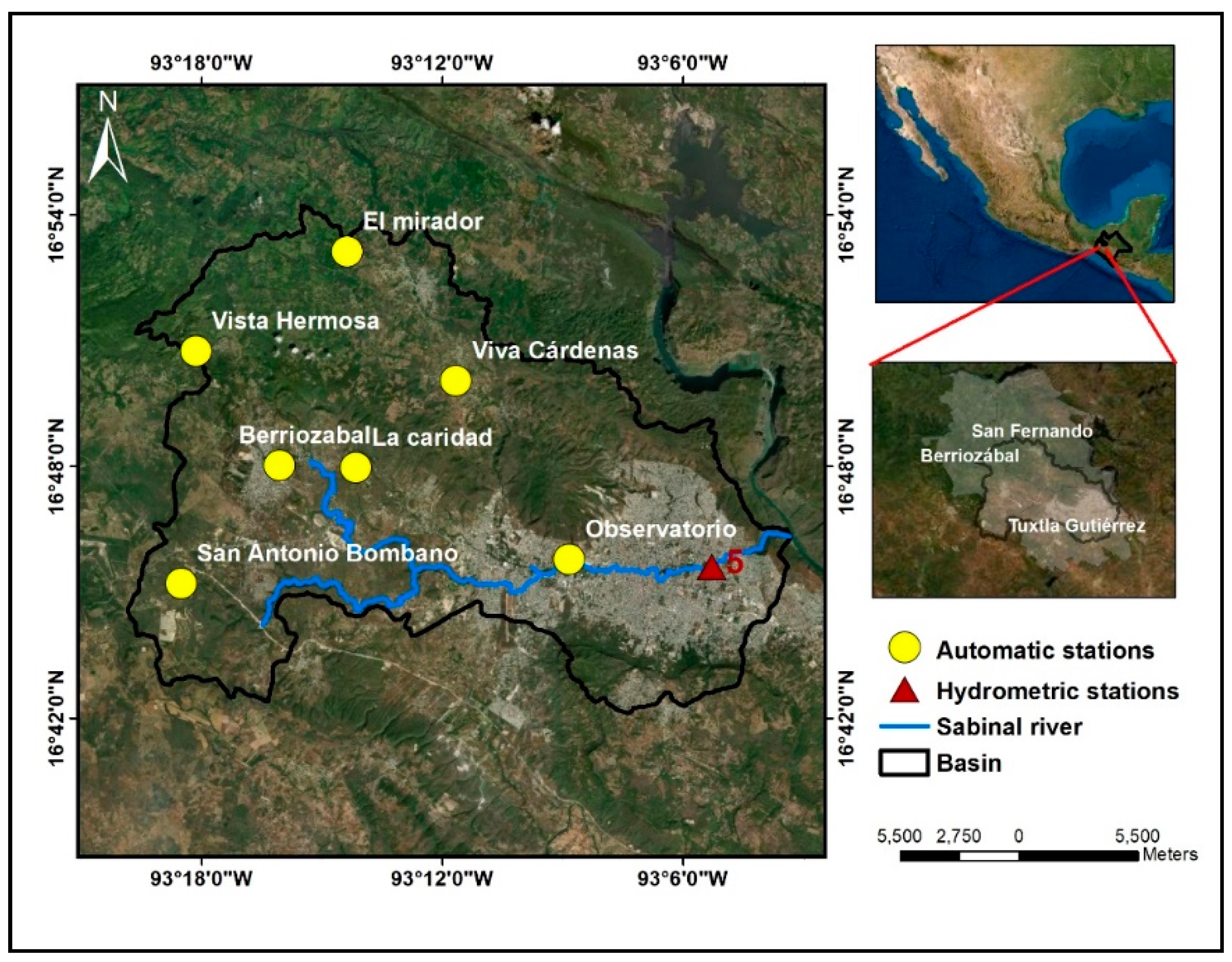
Figure 1.
Urban basin of Tuxtla Gutiérrez, Chiapas, México.
Figure 1.
Urban basin of Tuxtla Gutiérrez, Chiapas, México.
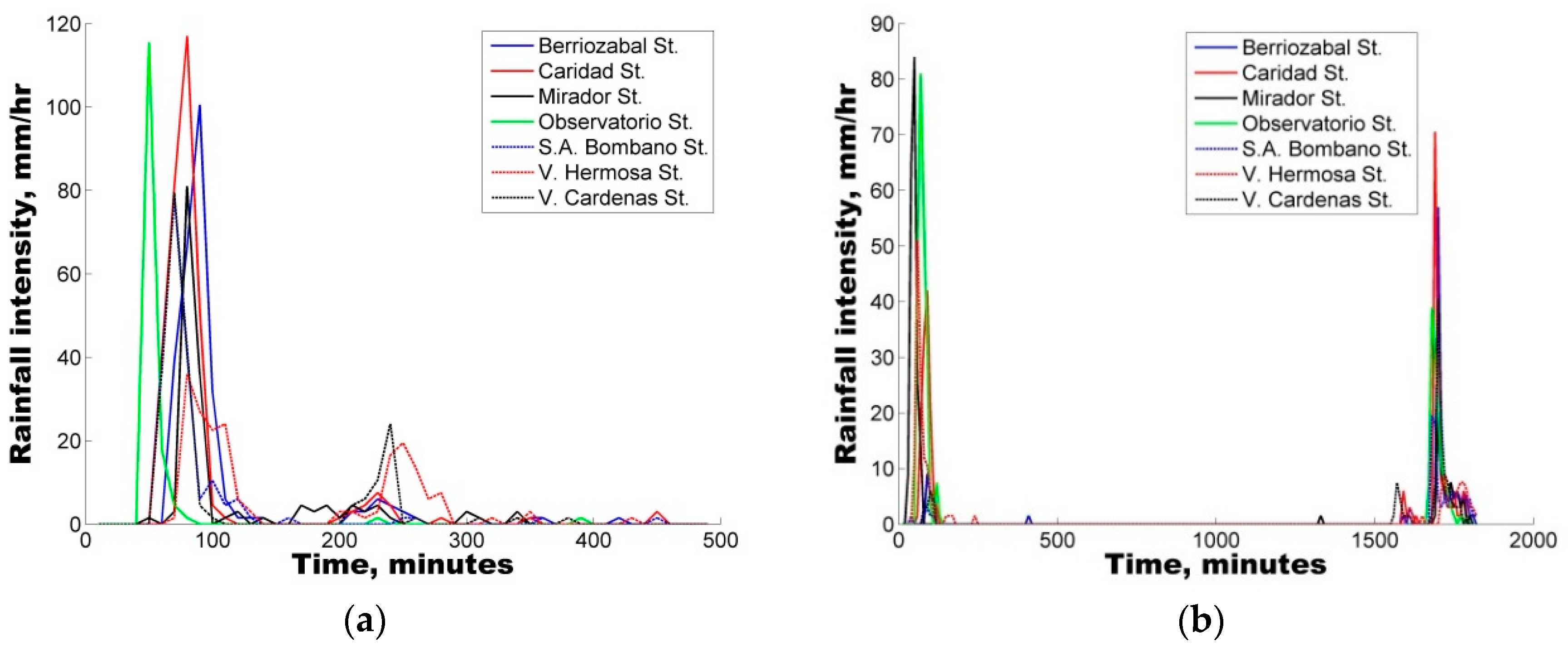
Figure 2.
(a) Precipitation Event 1 and (b) Precipitation Event 2.
Figure 2.
(a) Precipitation Event 1 and (b) Precipitation Event 2.
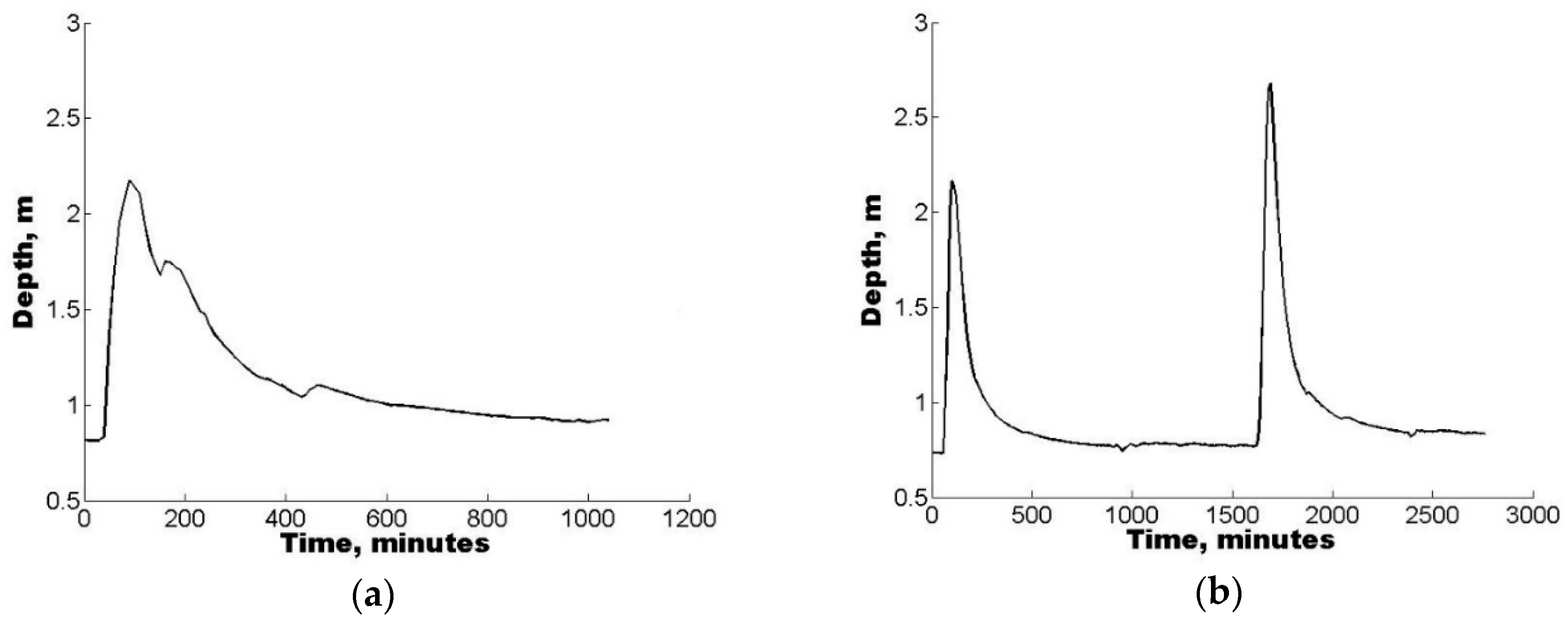
Figure 3.
Sabinal river hydrometry in Parque del Oriente station; (a) Event 1 and (b) Event 2.
Figure 3.
Sabinal river hydrometry in Parque del Oriente station; (a) Event 1 and (b) Event 2.
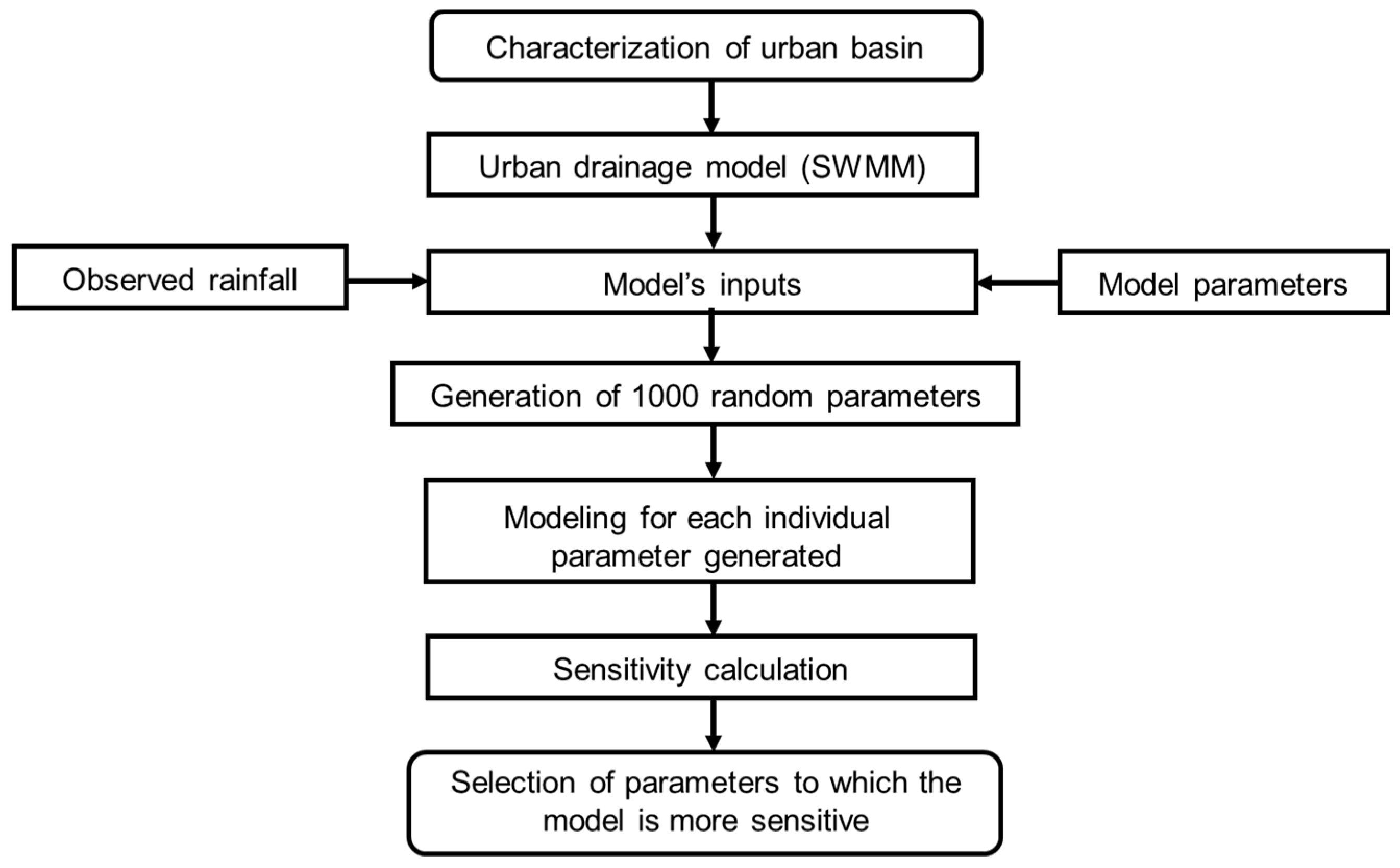
Figure 4.
Sensitivity analysis methodology.
Figure 4.
Sensitivity analysis methodology.
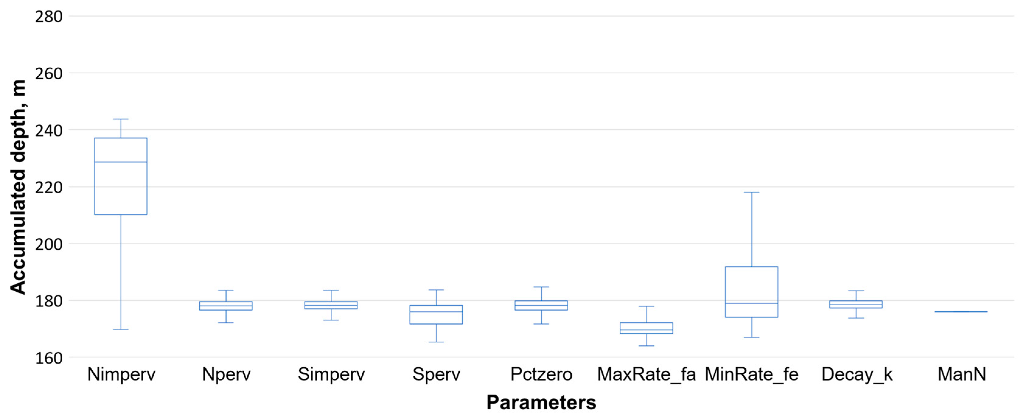
Figure 5.
Variation of the accumulated depth on the Sabinal River with respect to the parameters.
Figure 5.
Variation of the accumulated depth on the Sabinal River with respect to the parameters.
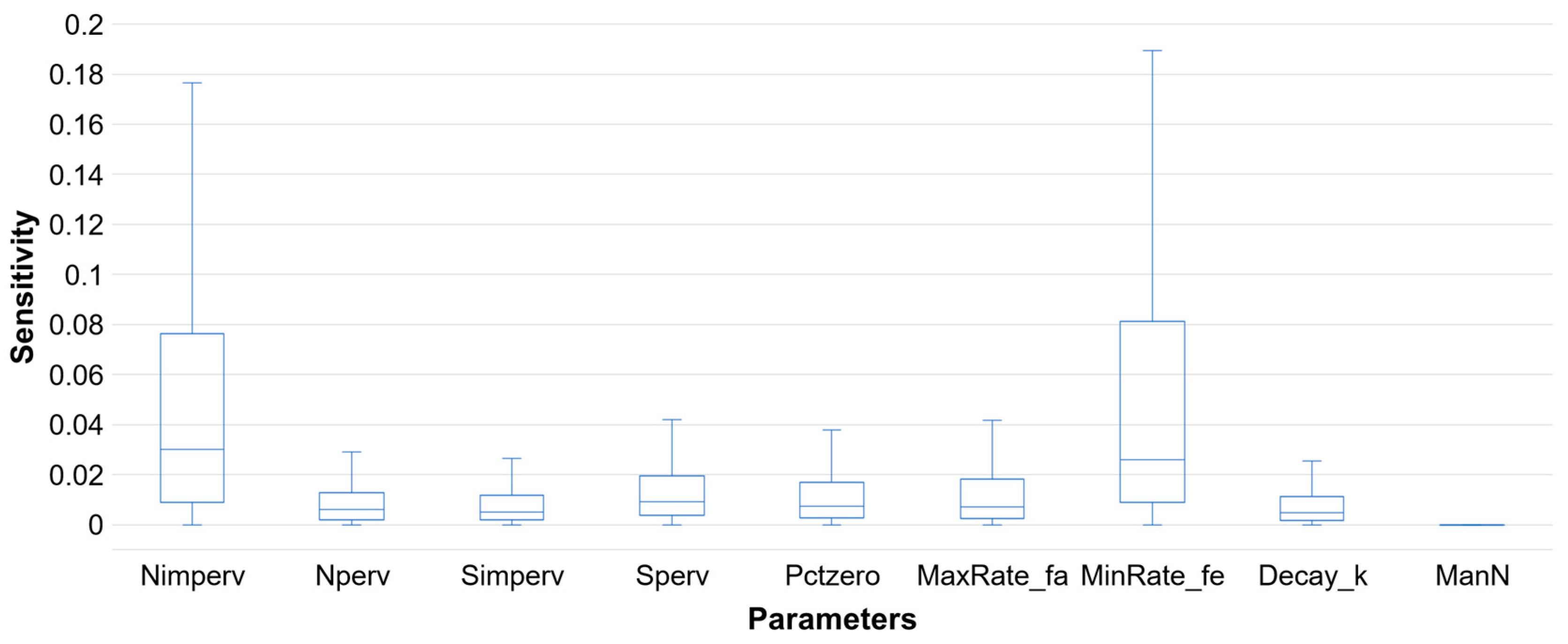
Figure 6.
Comparison of parameters with respect to the absolute–relative sensitivity index, Event 1.
Figure 6.
Comparison of parameters with respect to the absolute–relative sensitivity index, Event 1.
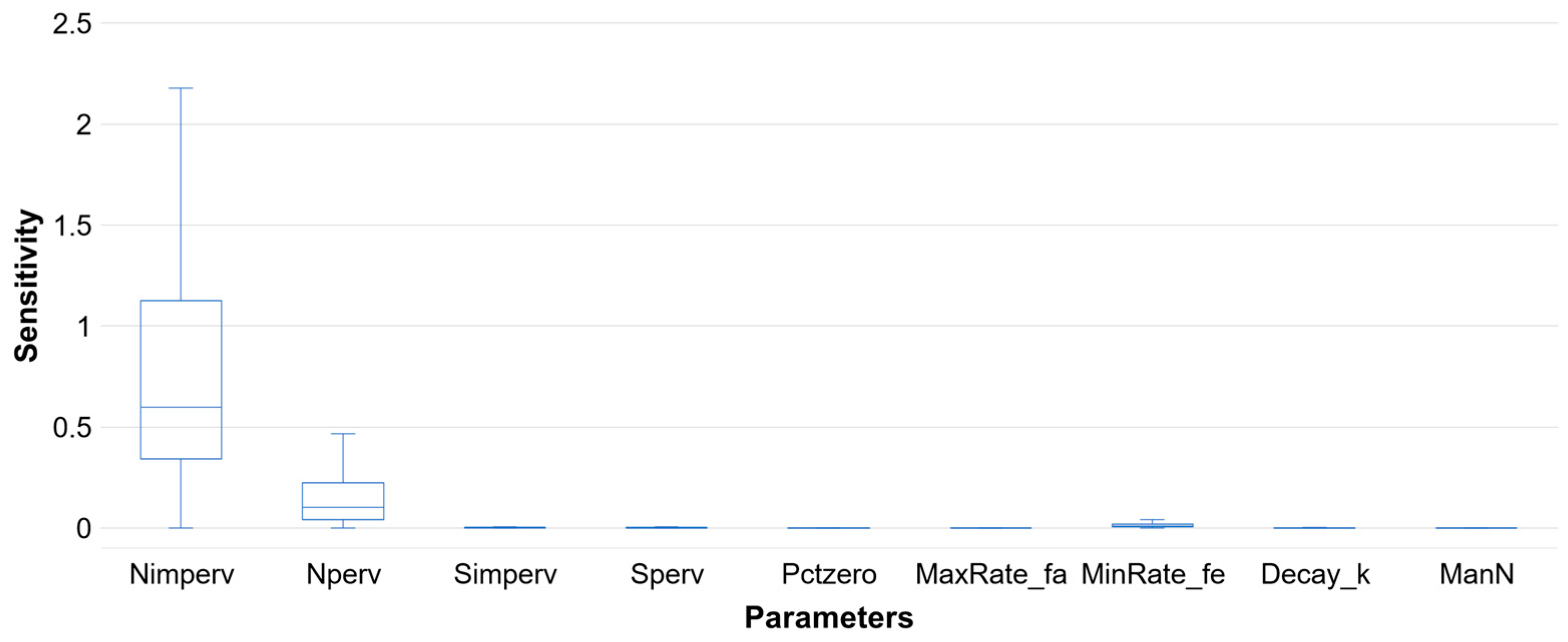
Figure 7.
Comparison of parameters with respect to the relative–absolute sensitivity index, Event 1.
Figure 7.
Comparison of parameters with respect to the relative–absolute sensitivity index, Event 1.
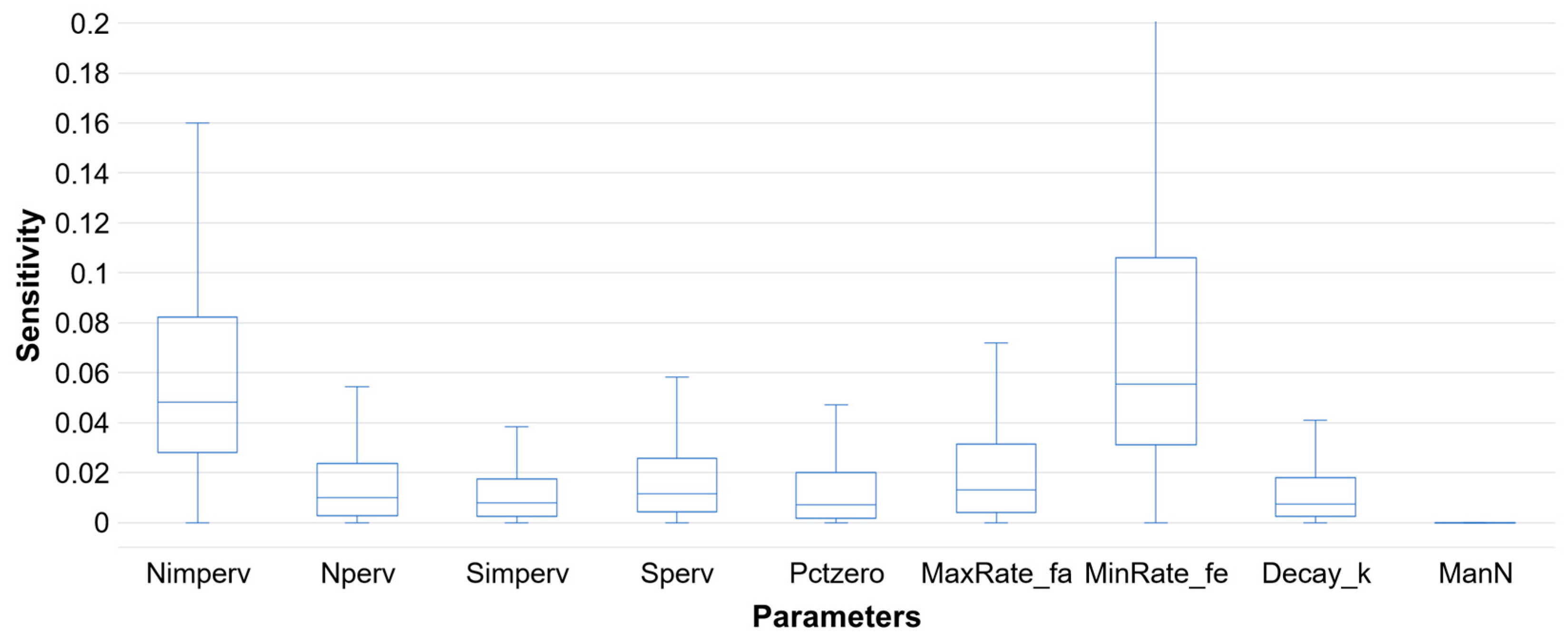
Figure 8.
Comparison of parameters with respect to the relative–relative sensitivity index, Event 1.
Figure 8.
Comparison of parameters with respect to the relative–relative sensitivity index, Event 1.
Figure 9.
(a) Average sensitivity of modeling parameters and (b) maximum sensitivity of modeling parameters, Event 1.
Figure 9.
(a) Average sensitivity of modeling parameters and (b) maximum sensitivity of modeling parameters, Event 1.
Figure 10.
Comparison of parameters with respect to R2, Event 1.
Figure 10.
Comparison of parameters with respect to R2, Event 1.
Figure 11.
Depth levels of Sabinal river using (a) Nimperv parameter and (b) MinRate_fe parameter. The blue line is a minimum value, the magenta line is an average value, the green line is a maximum value, the red line is a parameter with a maximum value of R2 and the black line is depth levels in hydrometric station.
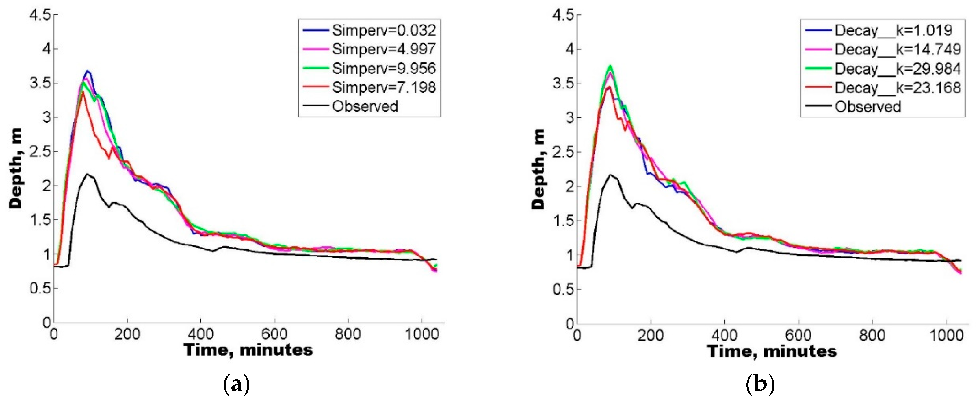
Figure 12.
Depth levels of Sabinal river using (a) Simperv parameter and (b) Decay_k parameter. The blue line is a minimum value, the magenta line is an average value, the green line is a maximum value, the red line is a parameter with maximum value of R2 and the black line is depth levels in hydrometric station.
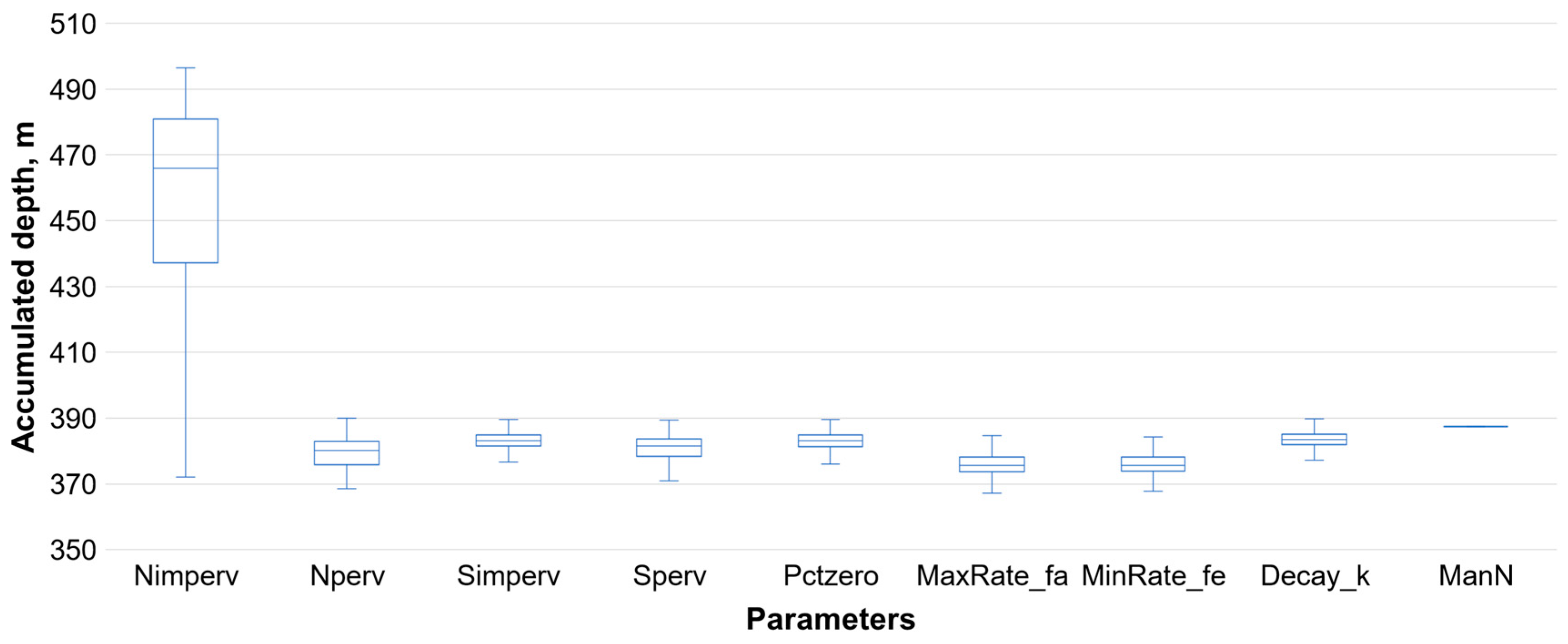
Figure 13.
Variation of the accumulated depth on the Sabinal River with respect to the parameters.
Figure 13.
Variation of the accumulated depth on the Sabinal River with respect to the parameters.
Figure 14.
Comparison of parameters with respect to the absolute–relative sensitivity index, Event 2.
Figure 14.
Comparison of parameters with respect to the absolute–relative sensitivity index, Event 2.
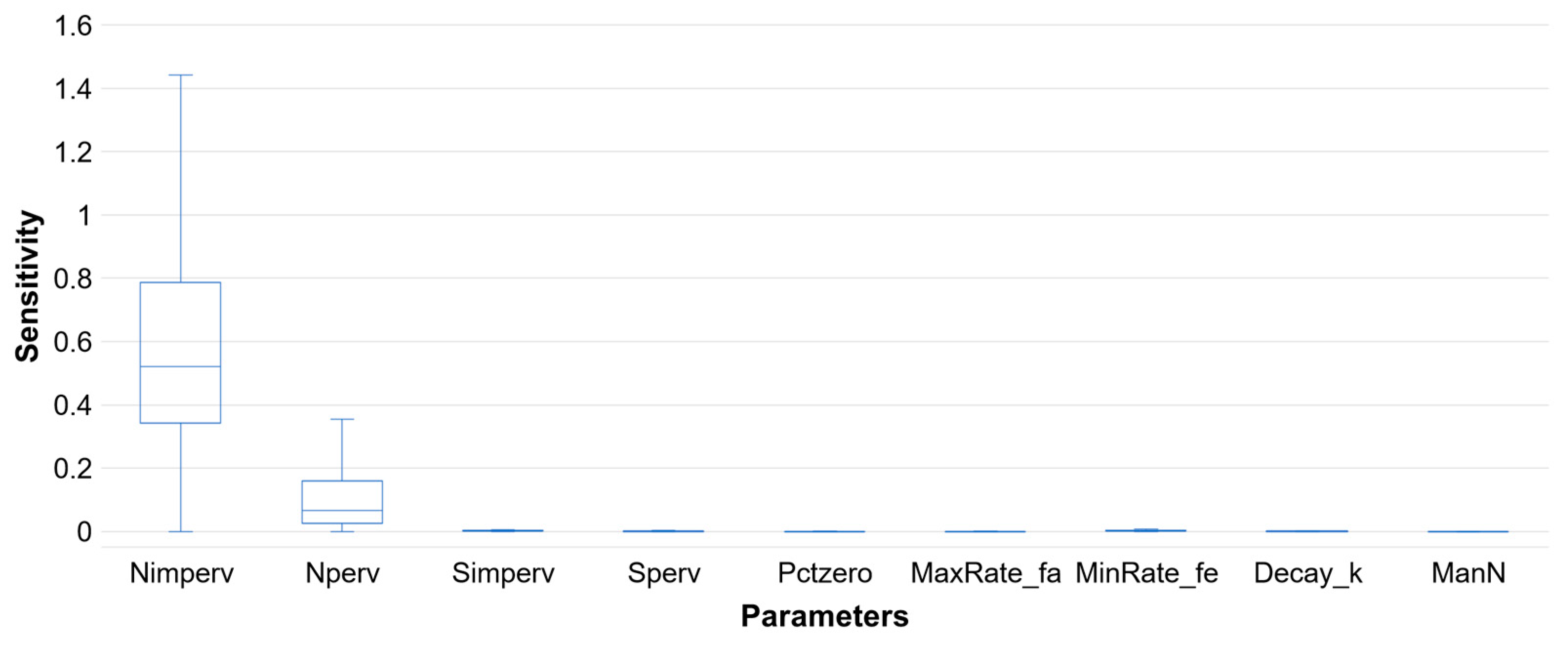
Figure 15.
Comparison of parameters with respect to the relative–absolute sensitivity index, Event 2.
Figure 15.
Comparison of parameters with respect to the relative–absolute sensitivity index, Event 2.
Figure 16.
Comparison of parameters with respect to the relative–relative sensitivity index, Event 2.
Figure 16.
Comparison of parameters with respect to the relative–relative sensitivity index, Event 2.
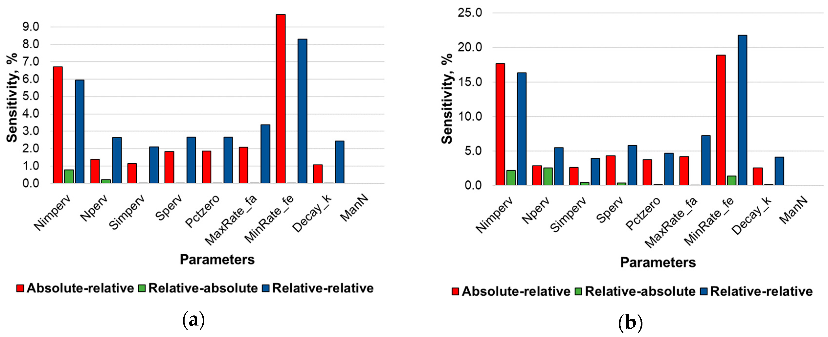
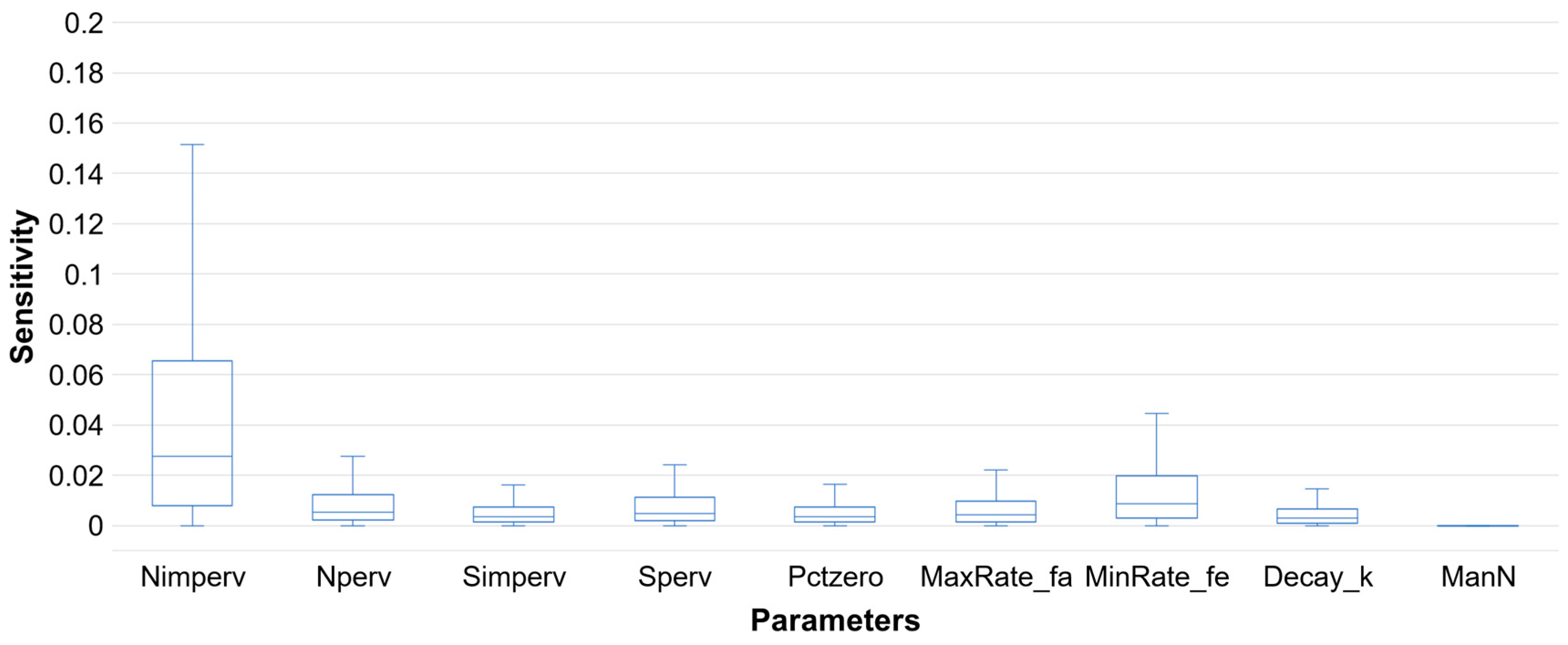
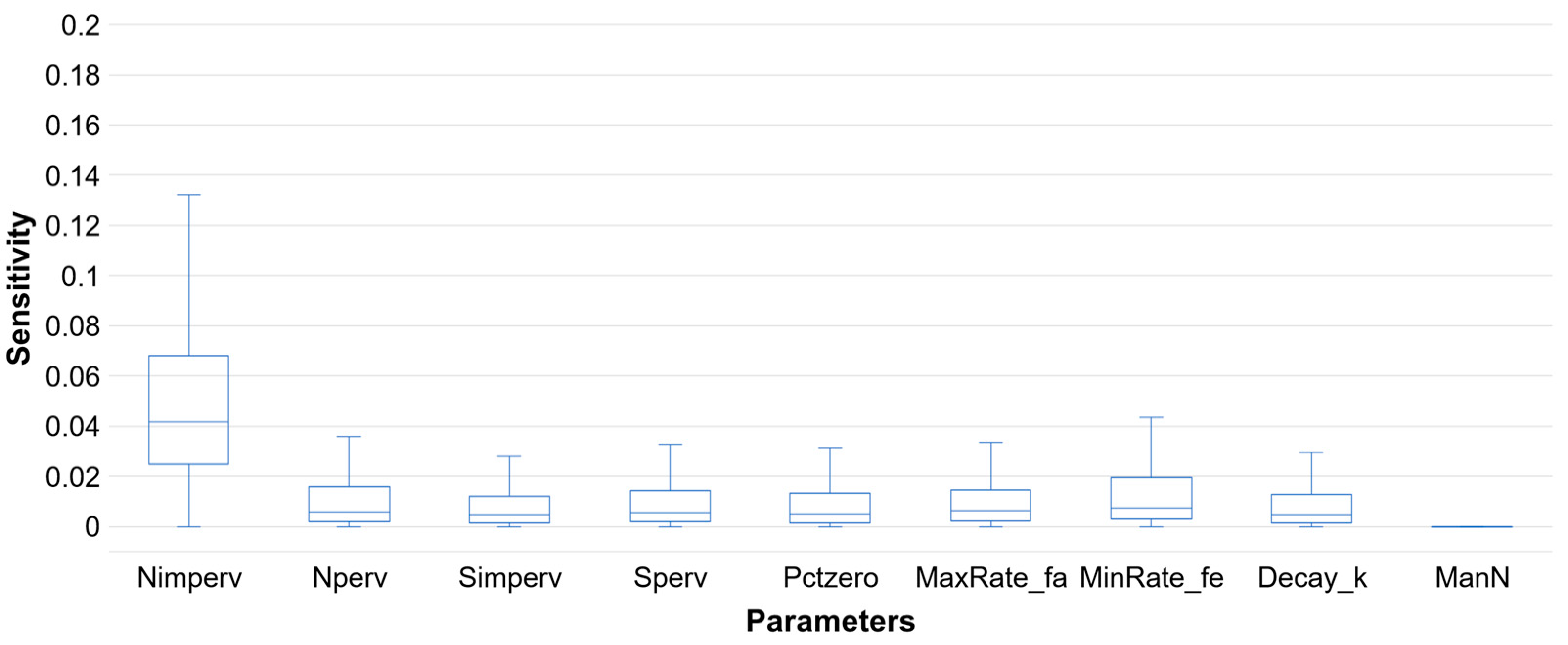
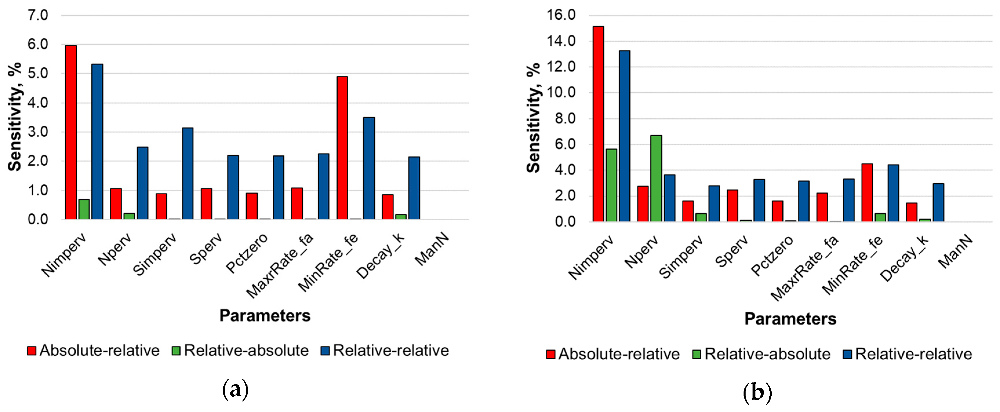
Figure 17.
(a) Average sensitivity of modeling parameters and (b) maximum sensitivity of modeling parameters, Event 2.
Figure 17.
(a) Average sensitivity of modeling parameters and (b) maximum sensitivity of modeling parameters, Event 2.
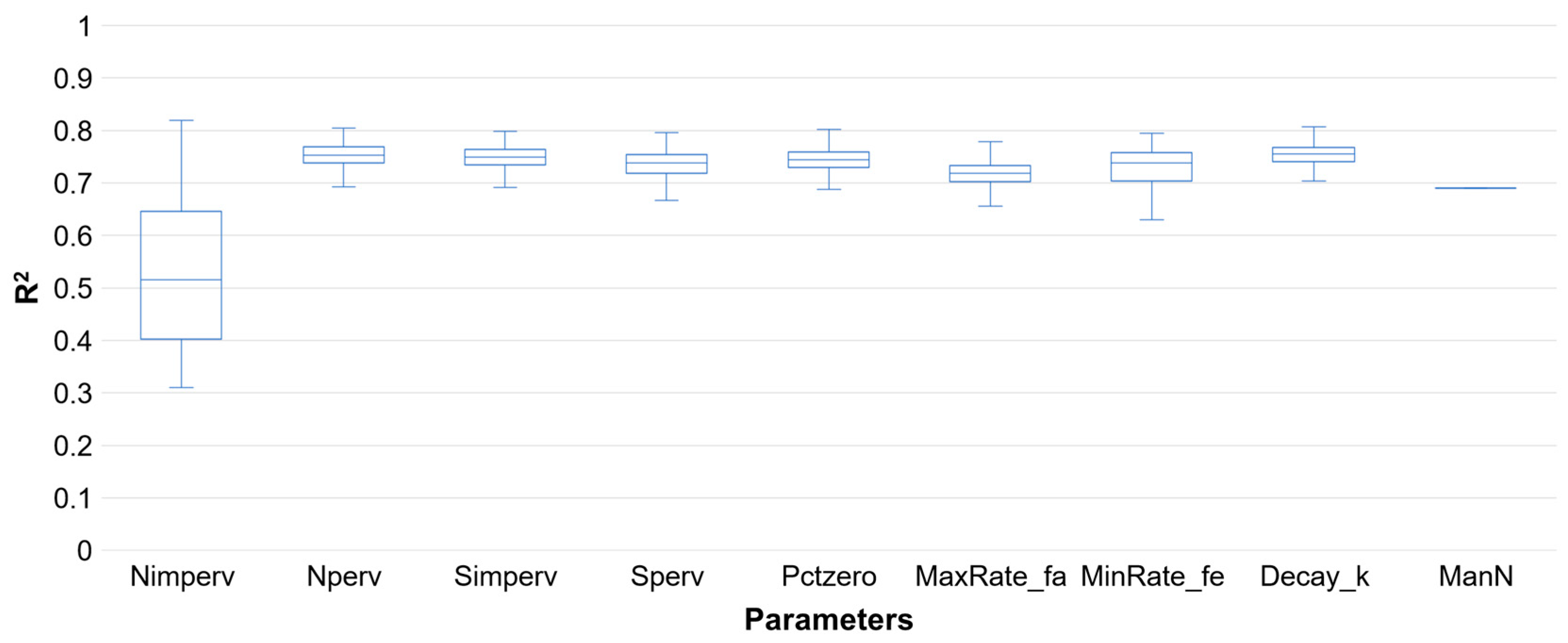
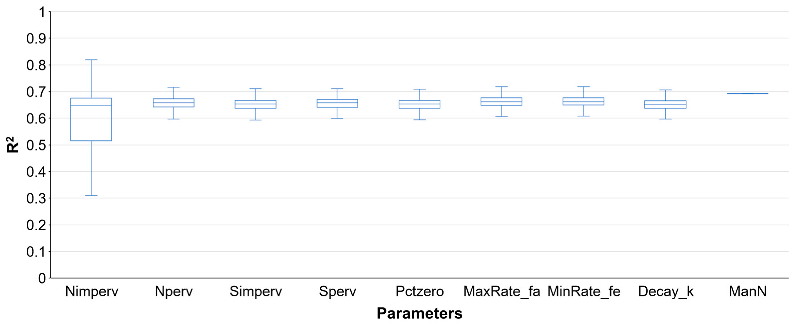
Figure 18.
Comparison of parameters with respect to R2, Event 2.
Figure 18.
Comparison of parameters with respect to R2, Event 2.
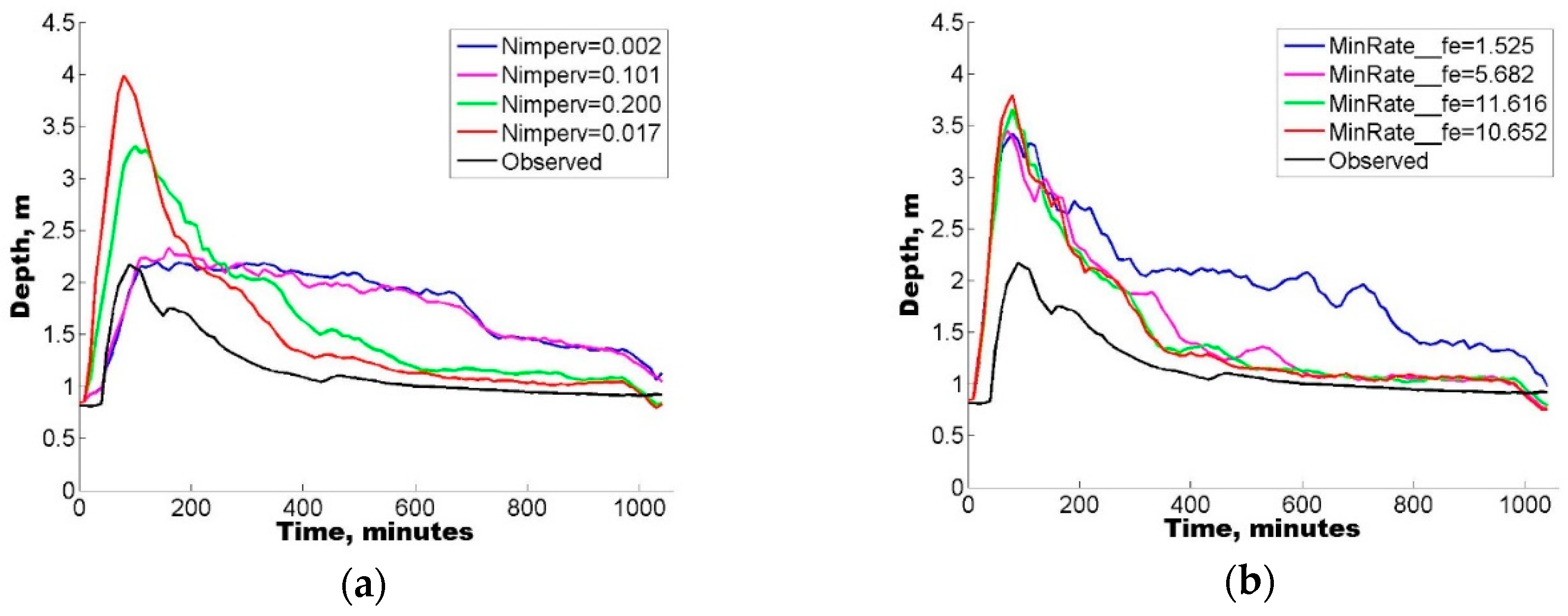
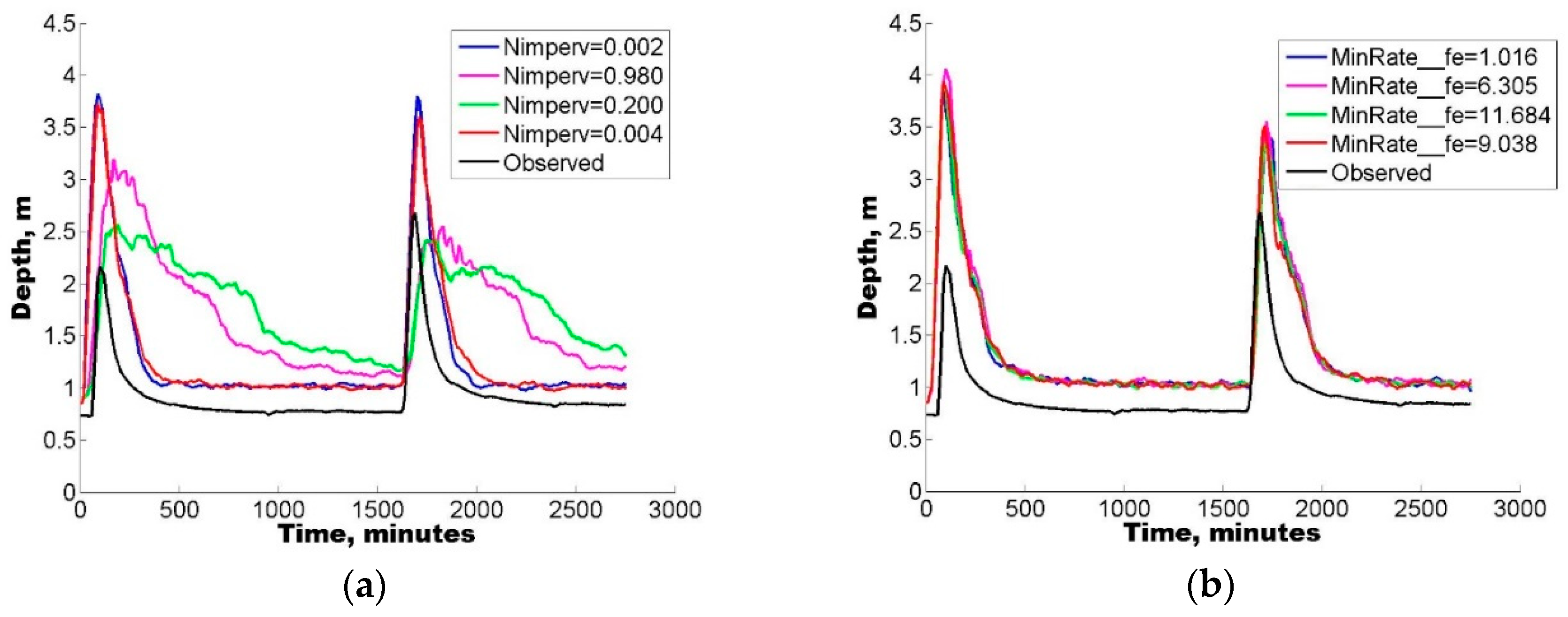
Figure 19.
Depth levels of Sabinal river using (a) Nimperv parameter and (b) MinRate_fe parameter. The blue line is a minimum value, the magenta line is an average value, the green line is a maximum value, the red line is a parameter with maximum value of R2 and the black line are depth levels in hydrometric station.
Table 1.
Precipitation characteristics, Event 1.
Table 1.
Precipitation characteristics, Event 1.
| Station | Duration (min) | Δt (min) | Maximum Intensity, (mm/h) | Accumulated Precipitation (mm) |
|---|
| Berriozábal | 490.00 | 10.00 | 100.50 | 45.50 |
| Caridad | 490.00 | 10.00 | 117.00 | 53.75 |
| Mirador | 490.00 | 10.00 | 81.00 | 27.00 |
| Observatorio | 490.00 | 10.00 | 115.50 | 23.75 |
| San Antonio Bombanó | 490.00 | 10.00 | 78.00 | 32.25 |
| Vista Hermosa | 490.00 | 10.00 | 36.00 | 33.25 |
| Viva Cárdenas | 490.00 | 10.00 | 79.50 | 35.75 |
Table 2.
Precipitation characteristics, Event 2.
Table 2.
Precipitation characteristics, Event 2.
| Station | Duration (min) | Δt, (min) | Maximum Intensity, (mm/h) | Accumulated Precipitation (mm) |
|---|
| Berriozábal | 1820.00 | 10.00 | 57.00 | 22.50 |
| Caridad | 1820.00 | 10.00 | 70.50 | 43.75 |
| Mirador | 1820.00 | 10.00 | 84.00 | 44.25 |
| Observatorio | 1820.00 | 10.00 | 81.00 | 58.75 |
| San Antonio Bombanó | 1820.00 | 10.00 | 19.50 | 16.50 |
| Vista Hermosa | 1820.00 | 10.00 | 51.00 | 32.00 |
| Viva Cárdenas | 1820.00 | 10.00 | 40.50 | 22.25 |
Table 3.
SWWM model parameters.
Table 3.
SWWM model parameters.
| Parameter | Abbreviation | Maximum Value | Minimum Value |
|---|
| Manning’s duct coefficient | ManN | 0.010 | 0.030 |
| Manning’s N for impervious area | Nimperv | 0.001 | 0.200 |
| Manning’s N for pervious area | Nperv | 0.010 | 0.200 |
| Depth of depression storage on impervious area, mm | Simperv | 0.000 | 10.000 |
| Depth of depression storage on pervious area, mm | Sperv | 0.000 | 20.000 |
| Percentage of impervious area with no depression storage, % | PctZero | 0.000 | 100.000 |
| Maximum infiltration rate, mm/hr | MaxRate_fa | 1.000 | 200.000 |
| Minimum infiltration rate, mm/hr | MinRate_fe | 1.000 | 25.000 |
| Decay coefficient, 1/hr | Decay_k | 1.000 | 30.000 |
Table 4.
Mean µ, standard deviation σ, and coefficient of variation Cv of the depth values with respect to the parameters, Event 1.
Table 4.
Mean µ, standard deviation σ, and coefficient of variation Cv of the depth values with respect to the parameters, Event 1.
| Parameter | µ (m) | σ (m) | Cv (%) |
|---|
| Nimperv | 221.30 | 19.85 | 8.97 |
| Nperv | 178.05 | 2.15 | 1.21 |
| Simperv | 178.31 | 1.96 | 1.10 |
| Sperv | 175.10 | 3.89 | 2.22 |
| PctZero | 177.75 | 3.23 | 1.82 |
| MaxRate_fa | 170.61 | 3.34 | 1.96 |
| MinRate_fe | 187.25 | 20.09 | 10.73 |
| Decay_k | 178.57 | 1.85 | 1.04 |
| ManN | 176.08 | 0.00 | 0.00 |
Table 5.
Mean µ, standard deviation σ and variance, σ2 of sensitivity values, Event 1.
Table 5.
Mean µ, standard deviation σ and variance, σ2 of sensitivity values, Event 1.
| Parameter | Absolute–Relative | Relative–Absolute | Relative–Relative |
|---|
| µ | σ | σ2 | µ | σ | σ2 | µ | σ | σ2 |
|---|
| Nimperv | 0.0670 | 0.1047 | 0.0110 | 0.7875 | 0.5723 | 0.3276 | 0.05945 | 0.04870 | 0.00237 |
| Nperv | 0.0139 | 0.0491 | 0.0024 | 0.2332 | 0.3961 | 0.1569 | 0.02644 | 0.06645 | 0.00442 |
| Simperv | 0.0116 | 0.0241 | 0.0006 | 0.0061 | 0.0262 | 0.0007 | 0.02112 | 0.05493 | 0.00302 |
| Sperv | 0.0184 | 0.0424 | 0.0018 | 0.0041 | 0.0192 | 0.0004 | 0.02677 | 0.05586 | 0.00312 |
| Pctzero | 0.0187 | 0.0419 | 0.0018 | 0.0009 | 0.0066 | 0.0000 | 0.02659 | 0.07668 | 0.00588 |
| Maxrate_fa | 0.0207 | 0.0695 | 0.0048 | 0.0007 | 0.0042 | 0.0000 | 0.03378 | 0.06498 | 0.00422 |
| Minrate_fe | 0.0970 | 0.2223 | 0.0494 | 0.0202 | 0.0660 | 0.0044 | 0.08293 | 0.08626 | 0.00744 |
| Decay_k | 0.0109 | 0.0240 | 0.0006 | 0.0026 | 0.0106 | 0.0001 | 0.02447 | 0.07148 | 0.00511 |
| ManN | 0.0000 | 0.0000 | 0.0000 | 0.0000 | 0.0000 | 0.0000 | 0.00000 | 0.00000 | 0.00000 |
Table 6.
Mean µ, standard deviation σ, and coefficient of variation Cv of the depth values with respect to the parameters, Event 2.
Table 6.
Mean µ, standard deviation σ, and coefficient of variation Cv of the depth values with respect to the parameters, Event 2.
| Parameter | µ (m) | σ (m) | Cv (%) |
|---|
| Nimperv | 455.74 | 32.47 | 7.12 |
| Nperv | 379.46 | 4.38 | 1.15 |
| Simperv | 383.17 | 2.60 | 0.68 |
| Sperv | 380.89 | 3.85 | 1.01 |
| PctZero | 383.11 | 2.66 | 0.69 |
| MaxRate_fa | 376.21 | 3.44 | 0.91 |
| MinRate_fe | 376.43 | 4.89 | 1.30 |
| Decay_k | 383.45 | 2.38 | 0.62 |
| ManN | 387.46 | 0.00 | 0.00 |
Table 7.
Mean, µ, standard deviation, σ, and variance, σ2, of sensitivity values, Event 2.
Table 7.
Mean, µ, standard deviation, σ, and variance, σ2, of sensitivity values, Event 2.
| Parameter | Absolute–Relative | Relative–Absolute | Relative–Relative |
|---|
| µ | σ | σ2 | µ | σ | σ2 | µ | σ | σ2 |
|---|
| Nimperv | 0.0596 | 0.1031 | 0.0106 | 0.6875 | 0.6241 | 0.3895 | 0.05345 | 0.05722 | 0.00327 |
| Nperv | 0.0107 | 0.0221 | 0.0005 | 0.2182 | 0.6057 | 0.3668 | 0.02482 | 0.10692 | 0.01143 |
| Simperv | 0.0090 | 0.0445 | 0.0020 | 0.0059 | 0.0323 | 0.0010 | 0.03140 | 0.20057 | 0.04023 |
| Sperv | 0.0107 | 0.0294 | 0.0009 | 0.0023 | 0.0090 | 0.0001 | 0.02197 | 0.10039 | 0.01008 |
| Pctzero | 0.0090 | 0.0415 | 0.0017 | 0.0005 | 0.0028 | 0.0000 | 0.02181 | 0.07978 | 0.00637 |
| Maxrate_fa | 0.0108 | 0.0321 | 0.0010 | 0.0002 | 0.0008 | 0.0000 | 0.02257 | 0.10334 | 0.01068 |
| Minrate_fe | 0.0490 | 0.3743 | 0.1401 | 0.0057 | 0.0305 | 0.0009 | 0.03501 | 0.23318 | 0.05437 |
| Decay_k | 0.0086 | 0.0340 | 0.0012 | 0.0017 | 0.0108 | 0.0001 | 0.02140 | 0.10890 | 0.01190 |
| ManN | 0.0000 | 0.0000 | 0.0000 | 0.0000 | 0.0000 | 0.0000 | 0.00000 | 0.00000 | 0.00000 |

 ,
, 


