Impact of Coastal Wetland Restoration Plan on the Water Balance Components of Heeia Watershed, Hawaii

Abstract

Optimal restoration and management of coastal wetland are contingent on reliable assessment of hydrological processes. In this study, we used the Soil and Water Assessment Tool (SWAT) model to assess the impacts of a proposed coastal wetland restoration plan on the water balance components of the Heeia watershed (Hawaii). There is a need to optimize between water needs for taro cultivation and accompanying cultural practices, wetland ecosystem services, and streamflow that feeds downstream coastal fishponds and reefs of the Heeia watershed. For this, we completed two land use change scenarios (conversion of an existing California grassland to a proposed taro field and mangroves to a pond in the wetland area) with several irrigation water diversion scenarios at different percent of minimum streamflow values in the reach. The irrigation water diversion scenarios aimed at achieving sustainable growth of the taro crop without compromising streamflow value, which plays a vital role in the health of a downstream fishpond and coastal environment of the watershed. Findings generally suggest that the conversion of a California grassland to a patched taro field is expected to decrease the baseflow value, which was a major source of streamflow for the study area, due to soil layer compaction, and thus decrease in groundwater recharge from the taro field. However, various taro irrigation water application and management scenarios suggested that diverting 50% of the minimum streamflow value for taro field would provide sustainable growth of taro crop without compromising streamflow value and environmental health of the coastal wetland and downstream fishponds.

1. Introduction

In the Hawaiian Islands, coastal wetlands represent a critical interface between terrestrial and ocean zones with a vital importance in terms of economic, cultural, and environmental values. As described by Mitsch and Gosselink [1], coastal wetlands naturally purify water from sediments and contaminants, transform nutrients, slow down the flow of freshwater from the mountains to the ocean, and provide suitable habitats both for flora and fauna, including a decrease in greenhouse emission through carbon sequestration processes and micro-climate mitigation. Coastal wetlands are also considered very attractive and agriculturally productive regions for tourists and residents. In addition, these regions play an important role against flooding, pollution, and the negative impacts of climate and land cover changes. They also act like a sponge by absorbing water during the wet season and releasing it through the dry season [2,3]. The important functionalities of coastal wetlands have motivated various research and management organizations to be more active in restoring and managing the natural resources of the coastal wetland. Furthermore, the recent financial and moral support of federal policies regarding preserving wetlands, such as “no net loss of wetlands in the United States”, has encouraged many non-profit organizations to restore the degraded wetlands [1]. In that direction, with support from the community and financial support from environmental conservation agencies, the non-profit Hawaii-based organization Kakoo Oiwi has committed to restoring the Heeia coastal wetland (HCW), which is located on the Island of Oahu, Hawaii.

The HCW is a typical example of degraded wetlands in Hawaii, where wetland restoration has been planned [4]. Before the 1950s, it was considered the most productive ecosystem for both marine and terrestrial food resources in Oahu [5]. After the 1950s, the HCW was overrun by the invasive California grass (Brachiara mutica) and lost most of its great ecological functionalities. The passive restoration approach (restoration based on nature’s work) cannot significantly restore the degraded wetland unless physical human interventions are directly employed to control various processes [6]. Consequently, human intervention for the coastal wetland restoration has paramount importance for the HCW. The recently proposed HCW restoration plan includes the conversion of about 69 hectares of wetland covered by California grass into organic wetland taro (Colocasia esculenta) and eight hectares of wetland mangroves to wetland sedges papyrus, which will serve as a convenience habitat for the native bird and a nursery site for juvenile fish [7]. The main issues of concern regarding the restoration activities of the HCW are related to the likely impacts on water availability, the future land cover change on the water balance components (WBCs), and setting the appropriate locations of restoration areas [8].

While the wetland restoration activities can improve the ecological functioning of a coastal wetland, they may have a considerable effect on the hydrologic cycle components of the watershed. For example, the wetland evaporates water more than other land use types, decreases air temperature through the evaporation process, sustains stream temperature (through shading, and the storage and release of cool water during dry season), and regulates the streamflow values [9]. Studies that assess the effect of restoration on the hydrologic cycle components are thus critical for developing informed decisions regarding restoration of coastal wetlands.

Among others, anthropogenic interventions and climate patterns are the effective drivers for land cover changes, which in turn modify the WBCs, including streamflow, evapotranspiration, and groundwater recharge [10]. Many studies have emphasized that anthropogenic land cover changes cause increases in runoff, lateral flow, and streamflow under high connectivity between surface and groundwater [11,12,13]. Tropical environments show a high sensitivity to land cover disturbances [14]. Land cover changes disturb the surface soil and decrease soil infiltration, which in turn causes high runoff and increases streamflow [15]. Therefore, such changes require a restoration procedure through the use of appropriate vegetation communities that are suitable for regional natural hydrologic conditions.

This study assessed the WBCs of the HCW under the current and future land cover conditions. The future land cover scenarios were formulated based on the Heeia Coastal Wetland Restoration (HCWR) plan [7]. In addition, the study investigated the land cover change impacts on the spatial and temporal variability of the hydrologic processes within the coastal wetland and its relationship with the hydrologic processes in the high-elevation area of the Heeia Watershed. To achieve these objectives, we used the Soil and Water Assessment Tool (SWAT) model [16]. The baseline results were used as a reference in quantifying the potential impacts of the HCWR plan on the WBCs of the watershed and coastal area.

2. Materials and Methods

2.1. Study Area

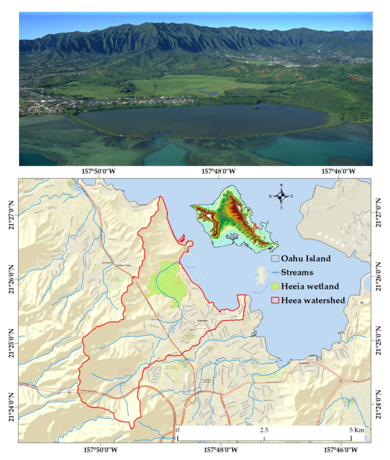
The Heeia wetland is the coastal part of the Heeia watershed, located on the windward side of the northeast coast of Oahu, representing the lower drainage basin of the watershed (Figure 1). Therefore, it is considered as a reservoir of freshwater originating from the springs in the mountains as surface water supplemented with lateral flow and baseflow. In the past, the watershed’s hydrologic features enabled the indigenous society to meet their food and resources needs from land and sea in a prized coastal region [17]. The elevation of the watershed ranges from 0 to 854 m above mean sea level (amsl) with an average slope of 40%, while the elevation of wetland ranges from 0 to 17 m amsl with an average slope of 5% [7].

The land use of the wetland is dominated by emergent wetland (77%), forested wetland (8%), shrub wetland (5%), evergreen (4%), and other land use (6%) (Figure 2). Currently, most of the wetland area is blanketed by the invasive California grass, while the forested wetland is covered by mangrove trees (https://coast.noaa.gov/ccapatlas/). While the proposed taro land use will cover the cultivated land, shrub wetland, and emergent wetland portion of the Heeia wetland portion, the proposed pond area will cover part of its forested wetland (Figure 2). Oahu’s historical land use is documented elsewhere (https://guides.library.manoa.hawaii.edu/c.php?g=704383&p=5000954), whereas the historical land use of the HCW, including its pre-development condition, is detailed in Kakoo Oiwi [7].

2.2. Available Data

The following data were used to construct a SWAT model and assess the WBCs of the Heeia watershed and coastal wetland:

• A 10 × 10 m Digital Elevation Model (DEM) obtained from the Department of Commerce (DOC), National Oceanic and Atmospheric Administration (NOAA), Center for Coastal Monitoring and Assessment (CCMA).
• A 1:24,000 scale soil map was obtained from the Soil Survey Geographic (SSURGO) database as provided by the US Department of Agriculture, Natural Resources Conservation Service (USDA-NRCS).
• A 2.4 × 2.4 m land use map data was downloaded from the NOAA Coastal Change Analysis Program (C-CAP), http://coast.noaa.gov/ccapftp/.
• As taro land use is not included in the crop database of SWAT, the specific plant parameters were obtained from actual field measurements and literature values [18,19,20,21,22,23,24,25].
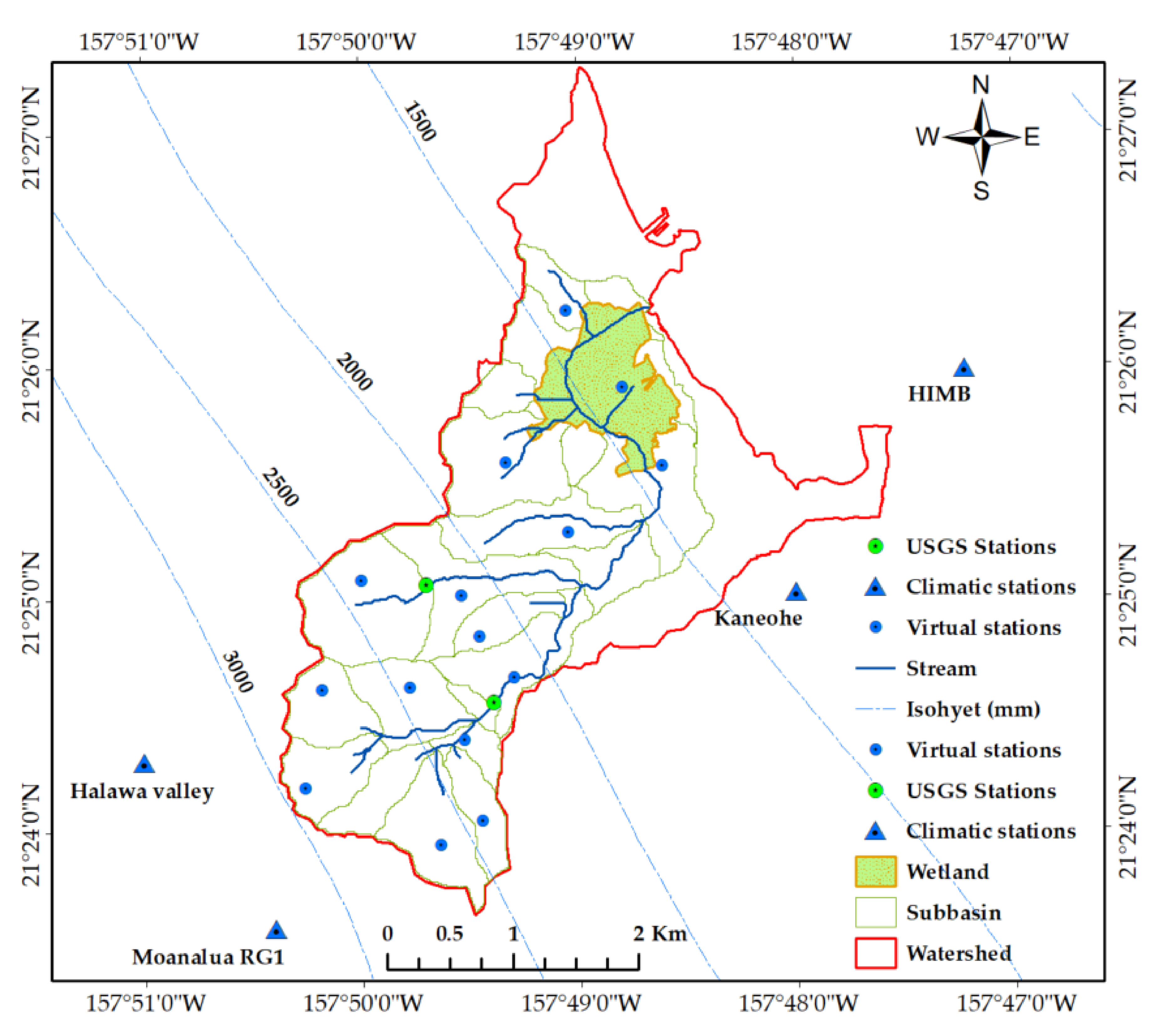
• Due to lack of hydro-meteorological data within the watershed, we utilized various approaches, including interpolation, rescaling, and estimation based on the observed data and contour maps. For instance, fifteen virtual stations (Figure 3) were created within the watershed based on the spatial variability of rainfall. Rainfall values were generated for each station using the closest rain gauge station and isohyets of the Rainfall Atlas of Hawaii [26]. To fill the other missing variables (temperature, wind speed, solar radiation, and relative humidity), a method proposed by Leta et al. [27] was used.
• Also used in the study is the daily streamflow data recorded at the Haiku station (U.S. Geological Survey (USGS) gauging station: 16275000) and others measured by this study at the coastal plain and estuary at the wetland flow sampling station for the period from 2012 to 2013. For the coastal plain, long-term and continuous streamflows were estimated based on the method developed by Leta et al. [27].

2.3. SWAT Model Description and Setup

SWAT is a physically based and semi-distributed hydrologic model that works at a basin scale and (sub-) daily time scale [16]. The applicability of SWAT has been widely proven in different hydrologic conditions, scales, and continents of the globe [28,29]. The model uses soil water balance concept and equations that consider precipitation as input and surface runoff, actual evapotranspiration, lateral flow, base flow, and deep groundwater loss as output at hydrological response units (HRUs) [30]. HRUs are the smallest spatial scale of the model representing a unique and homogeneous combination of soil, land use, and slope characteristics within a sub-basin, which is the second spatial scale of the model. Detailed approaches and equations used in SWAT for estimating the aforementioned water balance components at the HRUs level are provided in Reference [30].

We built up the SWAT model of the Heeia watershed based on the geo-spatial and hydro-meteorological data of the study area. By using the DEM data, we divided the watershed into 22 sub-basins. We captured the high spatial (topographic) variability of the watershed (Figure 1 and Figure 2) by using lower than the SWAT default threshold value (minimum drainage area) during sub-basin delineation as streamflow routing occurs at this level. We further sub-divided sub-basins into 984 HRUs based on similar combinations of land use, soil type, and slope. As this study focused on land use change impact assessments, we used zero threshold values for HRUs classification. We set up the model for the period from 1/1/2000 to 12/31/2014. We used the period from 2000 to 2001 as spin-up to initialize the state variables of the system, while we calibrated and validated the model for the period from 2002 to 2008 and 2009 to 2014, respectively.

In this study, we used the Soil Conservation Service Curve Number (SCS-CN) method for surface runoff simulations. We also used the Penman–Monteith method [31] option of SWAT for Potential Evapotranspiration estimation as that method is recommended for use in Hawaii’s climatic condition [32]. Finally, we used the variable storage routing method [33,34] option of SWAT for the daily simulated streamflow routing.

2.4. Model Sensitivity, Calibration, Validation, and Uncertainty Analysis

SWAT has been widely used to perform sensitivity, calibration, and uncertainty analysis (see, e.g., Reference [27]). We used the Sequential Uncertainty Fitting (SUFI-2) algorithm [35] for model calibration and uncertainty analysis. SUFI-2 also has an ability to account for all sources of uncertainties esteemed from model parameters, driving variables (e.g., rainfall), model structure, and calibration data (e.g., observed streamflow) [36]. We evaluated the total model uncertainty by using P and R factors [37]. The P-factor measures the percentage of measured data bracketed at a 95% prediction uncertainty band (95PPU), while the R-factor evaluates the average thickness of the 95PPU band divided by the standard deviation of the measured data (e.g., observed streamflow). The values of the P-factor and R-factor range between 0 to 1 and 0 to ∞, respectively. A P-factor of 1 and R-factor close to zero mean that the simulated values are exactly matching the observed values [37]. Finally, we performed a manual calibration to fine-tune the calibrated parameter values and obtain a reasonable agreement between observed and simulated WBCs [38]. Such an approach substantially reduces the time-consuming manual calibration, including easy quantitative and qualitative comparisons [39].

2.5. Model Performance Evaluation

We evaluated the performance of SWAT for daily streamflow simulation by using five evaluation criteria. These include the Nash–Sutcliffe efficiency (NSE) [40], the percent bias (PBIAS), the ratio of the root mean square error (RMSE) to the standard deviation of measured data (RSR), the root mean square error (RMSE) [41], the Mean Bias Error (MBE) [42], and the correlation coefficient (r) [43].

2.6. Land Cover Change Scenario

The HCWR plan (Figure 2) includes conversion of the California grass to organic wetland taro and the existing wetland mangrove forest to a pond as a native habitat for aquatic species. Based on the land use map data, the perennial California grassland mainly exists in the coastal wetland (Figure 2). It covers approximately 7% of the modeled area (8.5 km²). In addition, eight hectares of wetland mangrove forest (1% of the modeled area) is located around the Heeia stream estuary. The estuarine forested wetland in the C-CAP land use map of 2011 was treated as water during the land cover change conversion, while the California grassland was converted to taro cultivation. Taro was added to the SWAT crop database with the relevant properties that are summarized in

Table 1. Brief description of the variables in the Soil and Water Assessment Tool (SWAT) plant growth database file of wetland taro.

Variable Name	Code and Values	Definition	Reference
ICNUM	142	Land cover/plant code	This study
CPNM	TARO	Four character code of land name	This study
IDC	6	Herbaceous perennial crop code	[18,44]
CROPNAME	Wetland Taro	Name of flooded Taro	This study
BIO_E	47	Radiation-use efficiency of Herbaceous	[18,44]
HVSTI	0.01	Harvest index for optimal growth	This study
BLAI	2.5	Maximum potential leaf area index (LAI)	[25,44]
FRGRW1	0.11	Fraction of the plant growing season	[25,47]
LAIMX1	0.13	Fraction of the maximum LAI (first point)	[18,48]
FRGRW2	0.24	Fraction of the plant growing season	[18,25]
LAIMX2	0.91	Fraction of the maximum LAI (second point)	[18,25]
DLAI	0.89	Fraction of growing season (decline leaf area)	[18,25]
CHTMX	0.7	Maximum canopy height (meter)	This study
RDMX	0.6	Maximum root depth (meter)	This study
TOPT	25	Optimal temperature for plant growth (°C)	This study
TBASE	21	Minimum temperature for plant growth (°C)	This study

. These parameters were created based on the literature values [25] and field measurements. Also, some selected existing variables of herbaceous land use from the SWAT database were used for wetland taro because taro was classified as an herbaceous perennial tropical crop [44,45]. The taro crop is chosen in the restoration plan because it is an important staple food and spiritual plant in Hawaiian cultural heritage. Moreover, until the 1940s, the HCW was actively cultivated with taro [46] and the restoration plan is to revert the land to its original state.

2.7. Wetland Taro Management

The traditional system of producing flooded or wetland taro in Hawaii requires the crop to be flooded with water for 11 months. The main source of water is the stream, which is diverted to channels and individual taro patches. The farmers build a dam from soil and stone across the stream to create enough head for diverting water to the taro patches [19,49]. In order to reproduce this scheme in SWAT and to allow the inflow and outflow of water from the taro patches, we assumed and added a pothole to the taro’s management files of the SWAT model to simulate the HCW as a depressional water body. This enables to control the amount of water in the ditches of the taro field [50]. A pothole is a type of waterbody that obtains water from a sub-basin’s reach and releases it through overflow via tile drainage. The water balance for a pothole is defined by Neitsch et al. [30] as:

$$V=V_{stored}+V_{flowin}-V_{flowout}+V_{pcp}-V_{evap}-V_{seep}$$

(1)

where $V$ is the volume of stored water in the pothole at the end of the day (m³), $V_{stored}$ is the volume of initial stored water in the pothole at the beginning of the day (m³),$V_{flowin}$ is the volume of entered water to the pothole during the day (m³), $V_{flowout}$ is the volume of water flowing out of the water body during the day (m³), $V_{pcp}$ is the volume of precipitation falling on the pothole during the day (m³), $V_{evap}$ is the volume of water lost from the pothole by evaporation during the day (m³), and $V_{seep}$ is the volume of water lost from the pothole by seepage (m³).

The sources of water entering the pothole are from the sub-basin’s streamflow diversion to irrigate a given HRU within the sub-basin. Therefore, the inflow of water from reach to the pothole is calculated as:

$$V_{flowin}= irr+{\displaystyle \sum }_{hru=1}^n\left[f{r}_{pot , hru}·10·\left(Q_{surf, hru }+ Q_{gw, hru}+Q_{lat, hru}\right)·are{a}_{hru}\right]$$

(2)

where $V_{flowin}$ is the volume of water flowing into the pothole during the day (m³), irr is the amount of water irrigation diversion during the day (m³), n is the number of HRUs contributing water to the pothole, $f{r}_{pot , hru}$ is the fraction of the HRU area draining into pothole, $Q_{surf, hru }$is the water surface runoff from the HRU on a given day (mm), $Q_{gw, hru}$ is groundwater flow generated in the pothole on a given day (mm), $Q_{lat, hru }$is the water lateral flow generated in the pothole on a given day (mm), and $are{a}_{hru}$ is the HRU area (ha).

We assumed the whole HRUs of taro land use to be represented by a pothole. We also assumed that a maximum volume of water stored in a pothole is 40 mm (depth) over the entire HRU, with an initial volume of 10 mm (depth) and depth to impervious layer of 250 mm to cause water ponding for taro cultivation. For irrigation application, we defined a water diversion from a reach and irrigation water schedule in the management file of the taro land use. The necessary input parameters are summarized in

Table 2. The minimum flow, Qmin (m³/s), in the reach for different scenarios of irrigation water diversion.

Reach Number	S1	S2	S3	S4
1	0.02	0.01	0.005	0.002
2	1.5	0.75	0.375	0.15
3	1.5	0.75	0.375	0.15
4	0.06	0.03	0.015	0.006
5	1.6	0.8	0.4	0.16
6	0.06	0.03	0.015	0.006
7	0.2	0.1	0.05	0.02
8	2	1	0.5	0.2

Note: S1: scenario one (initial minimum streamflow, Qmin), S2: scenario two (50% of Qmin), S3: scenario three (25% of Qmin), S4: scenario four (10% Qmin).

. We controlled the amount of water diverted from a reach to a taro field by setting a minimum flow value in the reach. For instance, if the minimum flow value in the reach is set to high, the amount of diverted water to the taro field is low. Therefore, we started the irrigation water diversion scenario (S) with an initial high value (S1) and then decreased by 50% (S2), 75% (S3), and 90% (S4) of the minimum flow (Qmin) in the reach, respectively (Table 2).

3. Results and Discussion

3.1. Daily Streamflow Simulation and Uncertainty Analysis

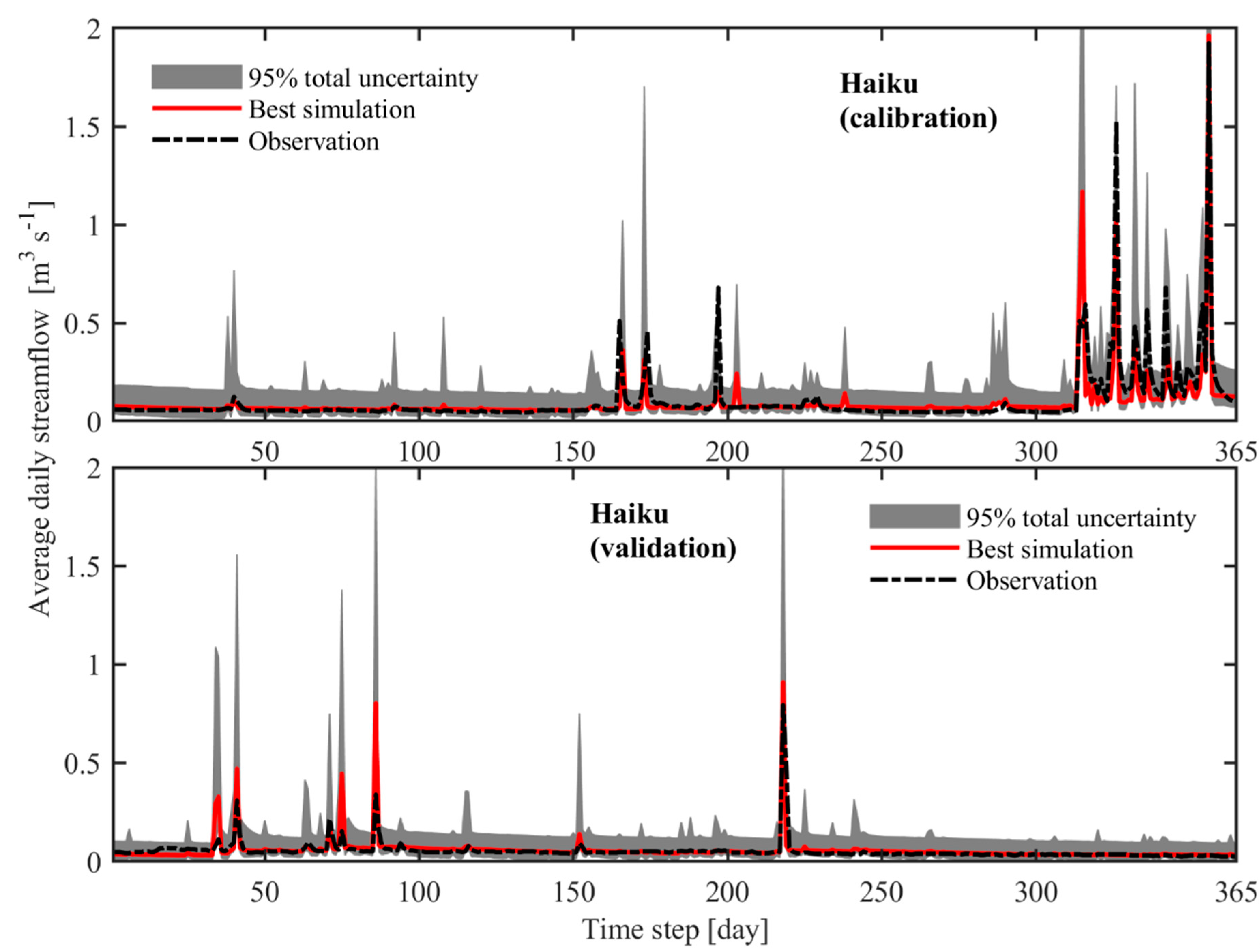
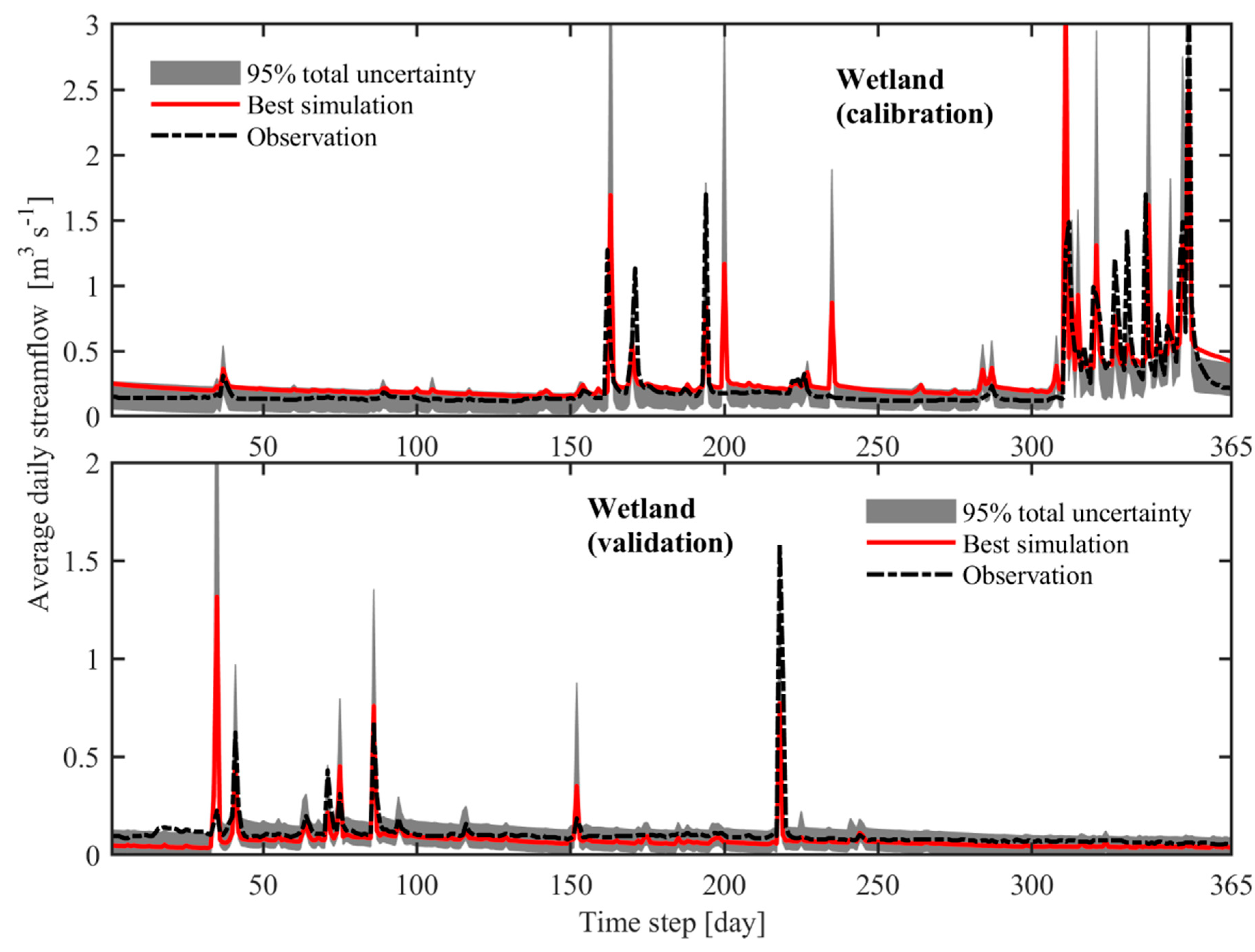
The model evaluation criteria for the daily streamflow values at both Haiku and Heeia wetland stations are summarized in

Table 3. Goodness-of-fit statistics of the Heeia watershed at Haiku and Wetland stations.

Station	Period	Time Span	NSE	PBIAS (%)	RSR	r	P-Factor	R-Factor
Haiku	Calibration	2002–2008	0.60	4.60	0.66	0.69	0.96	1.36
	Validation	2009–2014	0.51	8.00	0.70	0.54	0.96	0.89
Wetland	Calibration	2002–2008	0.51	13.00	0.63	0.67	0.81	0.81
	Validation	2009–2014	0.50	−2.59	0.67	0.50	0.95	0.67

Note: NSE = Nash–Sutcliffe Efficiency; PBIAS = Percent Bias; RSR = Root Mean Squared Error (RMSE) to observation Standard Deviation Ratio; r = Pearson correlation coefficient; P-factor = percent of observations bracketed in 95% prediction uncertainty (95PPU) confidence interval; R-factor = average width of the 95PPU interval.

. Table 3 shows that the model performance is within the generally accepted values for daily time-scale, considering the scarcity of the watershed data. Overall, based on the recommended quantitative statistics (NSE, RSR, and PBIAS), the model simulation could be judged as satisfactory because the averages of the three criteria were 0.53, 0.66, and 5.9 respectively, which are within the acceptable ranges for daily streamflow simulation [51,52].

The results of simulated and observed daily streamflows along with the 95% prediction uncertainty (95PPU) are presented in Figure 4 for the Haiku station and Figure 5 for the wetland station. The figures generally show that the SWAT model reasonably simulated the observed daily streamflows’ temporal evolution at both stations, except those simulated peak flow events when low observed flow values were recorded. The latter is most likely due to a lack of observed rainfall data within the watershed and high spatial rainfall gradient within a short distance (Figure 3). In addition, during the calibration period (2002–2008), 96% and 81% of the observed streamflow values were bracketed within the 95PPU at the Haiku and Wetland stations (Table 3), respectively. For the validation period (2009–2014), 96% of observed streamflow values were bracketed at the Haiku station, while 95% of the observed data were captured within the 95PPU at the wetland station. In addition, the R-factor values were close to 1 at both stations (Table 3), indicating that the model is reliable to simulate the Heeia watershed streamflow [53,54,55] and its applicability for future scenarios analysis.

3.2. The Watershed Water Balance

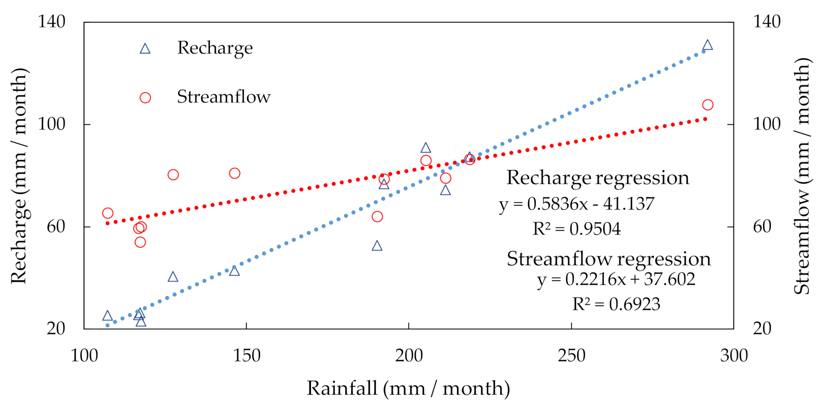
While the annual average rainfall over the entire Heeia watershed is 2043 mm for the period from 2002 to 2014, the amount over the wetland area is only about 1065 mm for the same period (

Table 4. The annual average of WBCs (all values in millimeters) for the Heeia wetland and watershed. LF = Lateral flow; BF = Base flow; ET = Evapotranspiration; PET = Potential Evapotranspiration (except rainfall, all are SWAT outputs).

Scale	Scenario	Rainfall	Streamflow	Runoff	LF	BF	Recharge	Soil Moisture	ET	PET
Wetland	baseline	1065	292	39	91	130	140	115	791	1533
	irrigation-S1	1065	313	62	137	76	82	144	792	1534
	irrigation-S2	1065	313	62	137	76	82	144	792	1534
	irrigation-S3	1065	314	63	138	76	82	144	793	1534
	irrigation-S4	1065	329	69	147	76	82	147	796	1534
Watershed	baseline	2043	904	119	306	459	699	171	916	1412
	irrigation-S1	2043	923	125	331	447	687	176	898	1412
	irrigation-S2	2043	923	125	331	447	687	176	898	1412
	irrigation-S3	2043	924	125	331	447	687	176	898	1412
	irrigation-S4	2043	932	129	336	447	687	177	900	1412

Note: S1 = Scenario one (initial minimum streamflow); S2 = Scenario two (decrease 50% of minimum streamflow); S3 = Scenario three (decrease 75% of minimum streamflow); S4 = Scenario four (decrease 90% of minimum streamflow).

). This noticeable annual rainfall spatial gradient is also clearly observed in Figure 3. As expected, the rainfall was high during the wet season (

Table 5. The average monthly (2002–2014) water balance components (all values in millimeters) of the Heeia watershed. LF = lateral flow; BF = base flow; WY = water yield; ET = evapotranspiration; PET = potential evapotranspiration (except rainfall, all are SWAT outputs).

Month	Rainfall	WY	Runoff	LF	BF	Recharge	Soil Moisture	ET	PET
Jan	192	79	10	31	35	77	179	61	91
Feb	205	86	19	31	34	91	176	63	95
Mar	292	108	23	43	40	131	179	83	109
Apr	127	80	5	31	42	41	148	96	124
May	146	81	10	25	44	43	126	95	129
Jun	107	66	4	18	42	25	104	89	142
Jul	118	60	2	15	41	23	101	82	145
Aug	117	60	3	16	39	26	100	75	144
Sep	117	54	3	14	36	27	104	69	130
Oct	190	64	8	19	36	53	135	70	115
Nov	211	79	15	29	34	75	155	69	98
Dec	219	86	16	33	36	88	171	62	89

) and highly correlated with recharge (R² = 0.95) (Figure 6). The percent of recharge comprised about 34% of the annual rainfall, which was consistent with previous studies in Hawaii [56,57]. The average annual water yield totaled 904 mm (Table 4). The baseflow contributed 87% of the average annual water yield while surface runoff contributed 6% (Table 4), indicating that water yield was highly influenced by the groundwater discharge due to the geological features of the study area [58]. The contribution of the baseflow was very strong during the dry season (May–October), as summarized in Table 5. In contrast, the stream received more surface runoff during the wet season (Table 5). The average annual potential evapotranspiration (PET) was 1412 mm whereas the actual evapotranspiration (AET) was 916 mm. AET was substantially lower than PET during the summer season because of the lack of sufficient soil moisture [59].

3.3. The Coastal Wetland Water Balance

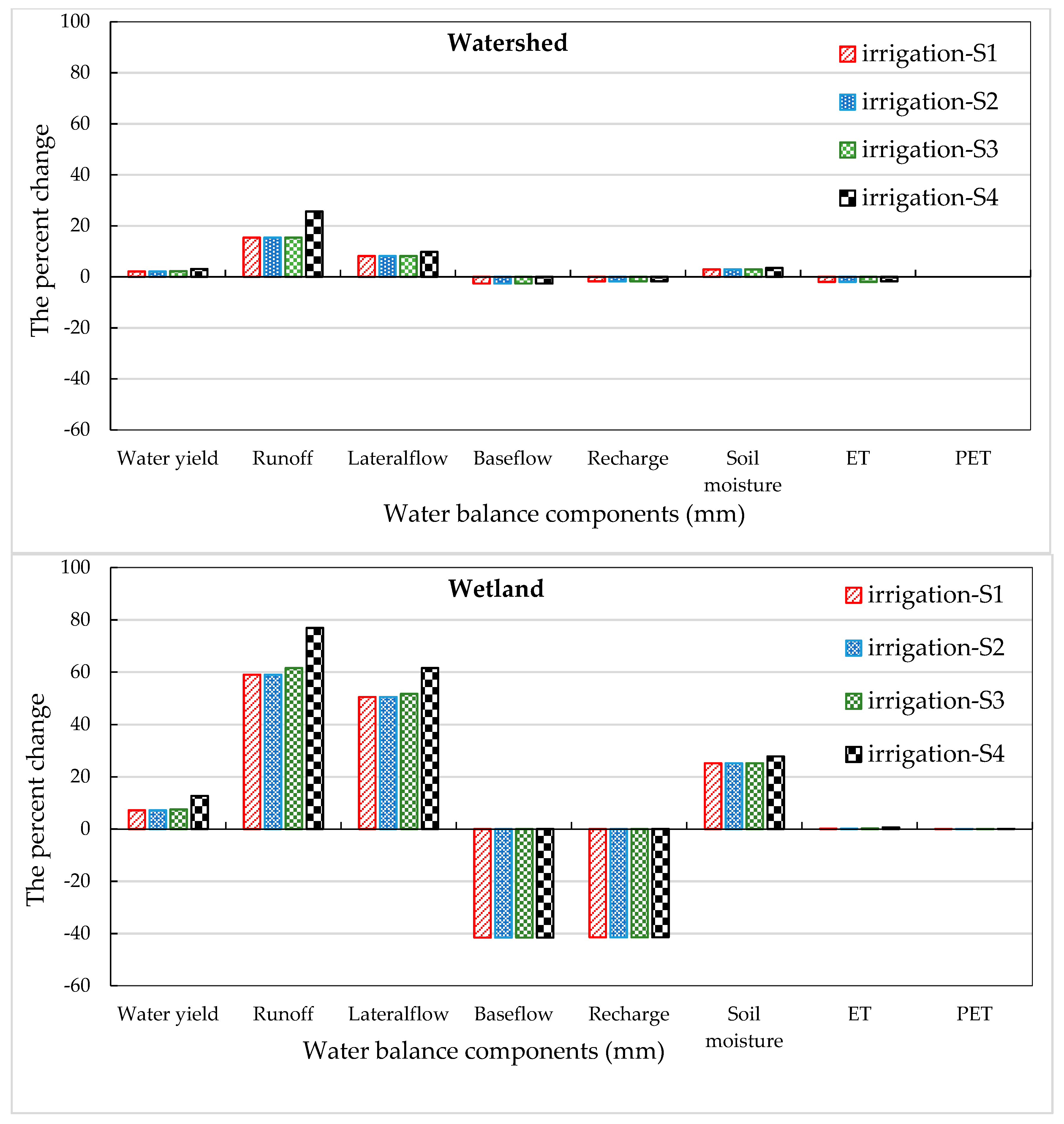
We evaluated the impacts of the HCWR plan (conversion of California grassland to taro field and mangroves to an impoundment) on WBCs at three spatial scales, which included the hydrologic response units (HRUs), sub-basins, and watershed. Under the HRUs scale, the restoration is expected to impact the annual WBCs (Figure 7). Specifically, the recharge will decrease due to the soil layer compaction under the taro patches to maintain ponding water in taro. However, the neighboring areas of the taro patches would get more recharge due to lateral seepage from the taro patches [50]. The AET is expected to increase, which may result in a decrease of the other WBCs and an increase in evaporation from the ponding water area. At the wetland scale, the results indicate that recharge is expected to decrease at least by 41% under all irrigation diversion scenarios, which is probably due to taro cultivation and water ponding management. In contrast, the lateral flow and surface runoff would increase by about 77% and 62% respectively, when 90% of the minimum streamflow is diverted (Figure 8). For this scenario, although baseflow is expected to decrease by up to 42%, water yield is predicted to increase by 13%, due to the considerable increase in surface runoff and lateral flow (Figure 8). We also noted that most of the WBCs were more affected during the dry season as compared to the wet season (

Table 6. The percent changes in the seasonal water balance components (WBCs) relative to the baseline for the Heeia Wetland and Watershed. LF = Lateral flow; BF = Base flow; ET = Evapotranspiration; PET = Potential Evapotranspiration (except rainfall, all are SWAT outputs).

Scale	Scenario	Season	Rainfall	Streamflow	Runoff	LF	BF	Recharge	Soil Moisture	ET	PET
Wetland	irrigation-S1	wet	0	18.94	80.19	40.5	−42.07	−41.42	23.97	−4.31	−0.27
		dry	0	−12.22	13.18	84.99	−41.37	−43.07	57.46	5.53	0.26
	irrigation-S2	wet	0	19.22	80.95	40.78	−42.07	−41.42	24.01	−4.29	−0.27
		dry	0	−12.17	13.32	85.22	−41.37	−43.07	57.49	5.54	0.26
	irrigation-S3	wet	0	19.86	82.64	41.46	−42.07	−41.42	24.13	−4.26	−0.27
		dry	0	−11.94	13.79	86.15	−41.37	−43.07	57.6	5.57	0.26
	irrigation-S4	wet	0	25.7	95.58	48.8	−42.07	−41.42	25.24	−3.94	−0.27
		dry	0	−5.62	35.46	108.34	−41.37	−43.07	59.95	6.21	0.26
Watershed	irrigation-S1	wet	0	2.29	6.86	5.72	−2.49	−2.01	3.05	−2.66	−0.06
		dry	0	1.93	1.85	12.3	−2.69	−0.98	5.1	−1.36	0.05
	irrigation-S2	wet	0	2.32	6.93	5.74	−2.49	−2.01	3.05	−2.66	−0.06
		dry	0	1.93	1.59	12.32	−2.69	−0.98	5.11	−1.36	0.05
	irrigation-S3	wet	0	2.39	7.16	5.83	−2.49	−2.01	3.09	−2.65	−0.06
		dry	0	1.95	1.66	12.37	−2.96	−0.98	5.13	−1.35	0.05
	irrigation-S4	wet	0	3.29	9.51	7.14	−2.94	−2.01	3.53	−2.5	−0.06
		dry	0	2.77	5.25	14.3	−2.69	−0.98	5.73	−1.12	0.05

Note: S1 = Scenario one (initial minimum streamflow); S2 = Scenario two (decrease 50% of minimum streamflow); S3 = Scenario three (decrease 75% of minimum streamflow); S4 = Scenario four (decrease 90% of minimum streamflow).

).

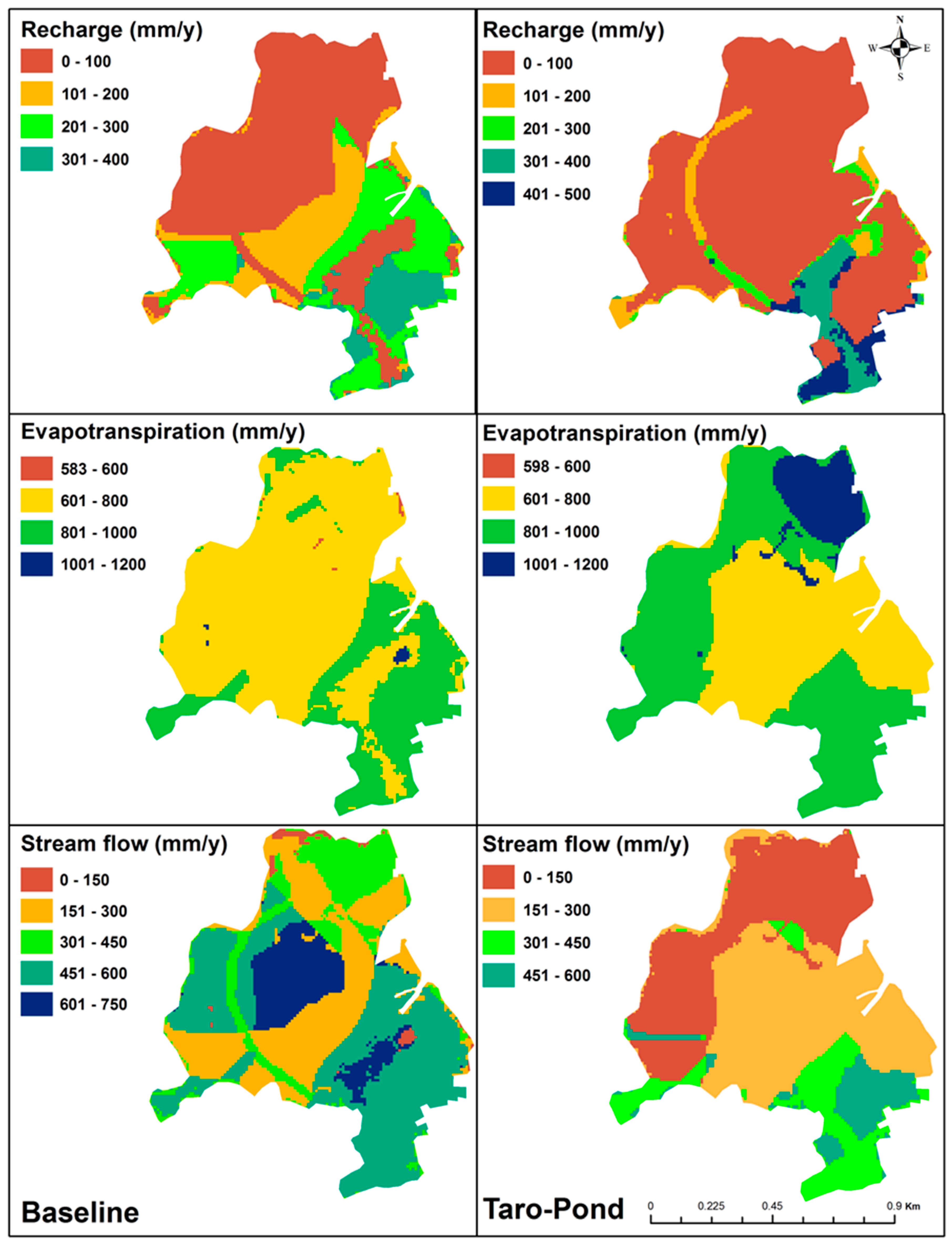
Finally, additional analysis on annual WBCs at the watershed scale indicated that the impact of land use change would have similar trends, but the relative percent change was low compared to the changes at sub-basin and HRU levels (Table 6). That should be expected considering the size of the taro cultivation area, which was relatively small in comparison with the watershed size. Another aspect of the research focused on the impact of land cover change on stream outflow for different scenarios of irrigation diversions. We did not apply irrigation water diversion for the baseline case, representing the initial condition without taro cultivation and pond creation. However, we implemented several irrigation water diversion scenarios from stream reaches to taro field by modifying the irrigation management parameter (minimum streamflow, FLOWMIN) in the management input files of the SWAT model. We set the FLOWMIN value to 50%, 75%, and 90% of the initial minimum value for each sub-basin within the wetland area. We referred to these scenarios as S1, S2, S3, and S4, respectively (Table 2).

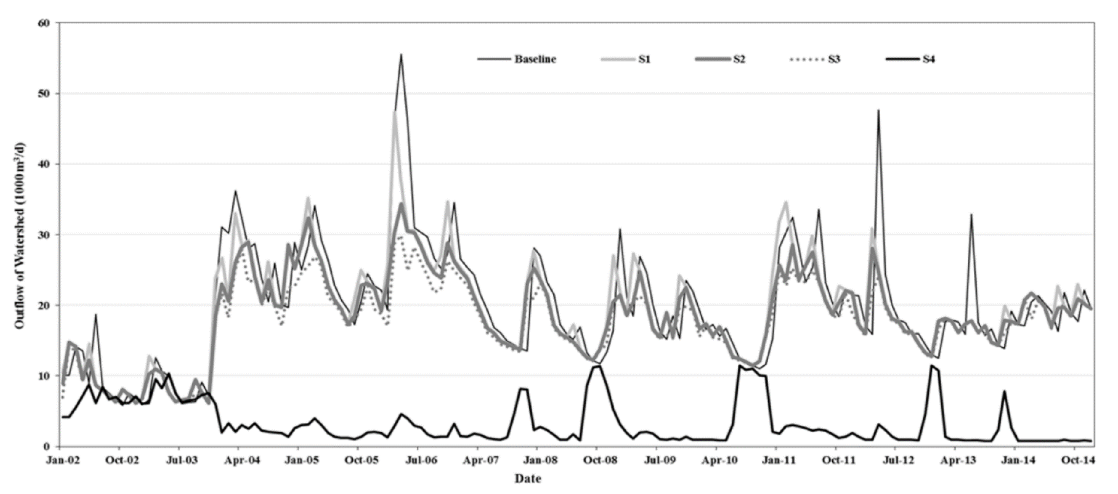
Figure 9 presents the monthly simulated streamflow values at the watershed outlet, just after the wetland area. The figure clearly indicates that all taro irrigation water diversion generally reduced stream outflows compared to the baseline values. However, as compared to the other scenarios, diverting 90% of minimum streamflow value (S4 scenario) significantly reduced the amount of outflows to the downstream. This highlights that excessively diverting irrigation water for the taro may negatively impact the downstream riverine ecosystem and environmental health, including the Heeia fishponds and reefs. Figure 9 further indicates that both S2 (50% minimum streamflow irrigation water diversion) and S3 (75% minimum streamflow irrigation water diversion) provide similar outflow values, which are close to S1, especially during the dry period. Although both S2 and S3 have similar impacts on the downstream outflow values, S2 outperformed S3 for two reasons: (i) S2 sufficiently supplied water for ponding and sustainably growing taro crop, and (ii) when compared to S3, S2 relatively showed a lower reduction in the downstream outflows that can play a vital role on the downstream fishponds and ecosystem services of the study area. Therefore, S2 is recommended to implement the proposed HCWR plan and achieve a sustainable growth of taro crop without compromising the coastal ecosystem role of the Heeia watershed.

4. Conclusions

In this study, we used the Soil and Water Assessment Tool (SWAT) model to assess the impacts of the proposed Heeia Coastal Wetland Restoration (HCWR) plan on the water balance components (WBCs). We successfully derived the majority of the climatic data of the model from nearby watersheds by using some scaling techniques to capture the spatial variability of the climate data, especially rainfall. Using sensitive parameters identified during sensitivity analysis, we calibrated and validated the SWAT simulated streamflow values against the observed streamflow values, including model prediction uncertainty.

The SWAT model reasonably represented the temporal variability of the observed daily streamflow hydrographs, with an acceptable performance and satisfactory statistical evaluation values under hydrologic data scarcity. The findings showed that 34% of the annual rainfall of the watershed (2043 mm) fed groundwater as recharge (699 mm), 15% of the annual rainfall went as lateral flow (307 mm), 6% of the annual rainfall went as runoff (119 mm), and actual evapotranspiration (AET) accounted for 45% the annual rainfall (917 mm). In addition, baseflow and lateral flow contributed 87% of the annual water yield. The baseflow was found to be the main component of the water yield compared with surface runoff.

The impacts of the HCWR plan on WBCs is expected to be significant for the wetland area. Additionally, the restoration plan is predicted to reduce the recharge and baseflow values, but to increase lateral flow and surface runoff values. We completed different irrigation water diversion scenarios to taro field to identify an optimal policy to achieve sustainable growth of the taro crop without compromising the streamflow values in the mainstream and at the downstream fishponds that play a vital role in the downstream coastal ecology of the study area. We concluded that an optimal management strategy for the wetland and coastal shoreline restoration of the study area is possible by sustaining streamflow as well as water needs for the taro patches. Based on the findings, the study proposed to use 50% of the minimum streamflow value for irrigation water diversion to irrigate the taro field.

References

- Mitsch, W.J.; Gosselink, J.G. Wetlands, 4th ed.; John Wiley & Sons, Inc.: New York, NY, USA, 2007. [Google Scholar]
- Bantilan-Smith, M.; Bruland, G.L.; MacKenzie, R.A.; Henry, A.R.; Ryder, C.R. A comparison of the vegetation and soils of natural, restored, and created coastal lowland wetlands in Hawaii. Wetlands 2009, 29, 1023–1035. [Google Scholar] [CrossRef]
- Bruland, G. Coastal wetlands: Function and role in reducing impact of land-based management. Coast. Watershed Manag. 2008, 13, 85. [Google Scholar]
- Henry, A.R. Strategic Plan for Wetland Conservation in Hawaii; Pacific Coast Joint Venture: Honolulu, HI, USA, 2006. [Google Scholar]
- Kailua Bay Advisory Council. Ko’olaupoko Watershed Restoration Action Strategy Kailua Bay Advisory Council (KBAC); Hawaii’s Department of Health: Honolulu, HI, USA, 2007. [Google Scholar]
- Jaradat, A. Agriculture in Iraq: Resources, potentials, constraints, and research needs and priorities. Food Agric. Environ. 2003, 1, 160–166. [Google Scholar]
- Oiwi, K. Heeia Wetlands Restoration, File Number: POH-2010-00159; Townscape, Inc: Käneÿohe, HI, USA, 2011. [Google Scholar]
- Oiwi, K. Heeia Wetland Restoration Strategic Plan 2010–2015; Käneÿohe, HI, USA, 2010; p. 16. [Google Scholar]
- Abu Hammad, A.; Tumeizi, A. Land degradation: Socioeconomic and environmental causes and consequences in the eastern Mediterranean. Land Degrad. Dev. 2012, 23, 216–226. [Google Scholar] [CrossRef]
- Shamrukh, M. Assessment of riverbank filtration for potable water supply in upper egypt. J. Eng. Sci. 2006, 34, 1175–1184. [Google Scholar]
- Ghodeif, K.; Paufler, S.; Grischek, T.; Wahaab, R.; Souaya, E.; Bakr, M.; Abogabal, A. Riverbank filtration in Cairo, Egypt—part I: Installation of a new riverbank filtration site and first monitoring results. Environ. Earth Sci. 2018, 77, 270. [Google Scholar] [CrossRef]
- Martin-Jézéquel, V.; Hildebrand, M.; Brzezinski, M.A. Silicon metabolism in diatoms: Implications for growth. J. Phycol. 2000, 36, 821–840. [Google Scholar] [CrossRef]
- Simpson, T.L.; Volcani, B.E. Silicon and Siliceous Structures in Biological Systems; Springer Science & Business Media: Berlin/Heidelberg, Germany, 2012. [Google Scholar]
- Bruijnzeel, L. Hydrological Impacts of Converting Tropical Montane Cloud Forest to Pasture, with Initial Reference to Northern Costa Rica; Final Technical Report DFID-FRP Project no. R7991; Vrije Universiteit: Amsterdam, The Netherlands, 2006. [Google Scholar]
- Schmidt, C.K.; Lange, F.; Brauch, H.; Kühn, W. Experiences with riverbank filtration and infiltration in Germany. DVGW-Water Technol. Cent. (TZW) Karlsr. Ger. 2003, 1–17. [Google Scholar]
- Arnold, J.G.; Srinivasan, R.; Muttiah, R.S.; Williams, J.R. Large area hydrologic modeling and assessment part I: Model development. AWRA J. Am. Water Resour. Assoc. 1998, 34, 73–89. [Google Scholar] [CrossRef]
- Hunter, C.L.; Evans, C.W. Coral reefs in Kaneohe Bay, Hawaii: Two centuries of western influence and two decades of data. Bull. Mar. Sci. 1995, 57, 501–515. [Google Scholar]
- Arnold, J.; Kiniry, J.; Srinivasan, R.; Williams, J.; Haney, E.; Neitsch, S. Soil and Water Assessment Tool Input/Output File Documentation: Version 2012; Technical Report; Texas Water Resources Institute: College Station, TX, USA, 2012. [Google Scholar]
- Gingerich, S.B.; Yeung, C.W.; Ibarra, T.-J.N.; Engott, J.A. Water Use in Wetland Kalo Cultivation in Hawaii; U. S. Geological Survey: Reston, VA, USA, 2007.
- Mat, N.; Hamzah, Z.; Maskin, M.; Wood, A.K. Mineral uptake by taro (colocasia esculenta) in swamp agroecosystem following gramoxone®(paraquat) herbicide spraying. J. Nucl. Relat. Technol. 2006, 3, 59–68. [Google Scholar]
- Onwueme, I. Taro cultivation in Asia and the Pacific. Rap Publ. 1999, 16, 1–9. [Google Scholar]
- Penn, D.C. Water and Energy Flows in Hawaii Taro Pondfields; University of Hawaii at Manoa: Honolulu, HI, USA, 1997. [Google Scholar]
- Nejadhashemi, A.P.; Shen, C.; Wardynski, B.J.; Mantha, P.S. Evaluating the impacts of land use changes on hydrologic responses in the agricultural regions of Michigan and Wisconsin. In Proceedings of the 2010 American Society of Agricultural and Biological Engineers, Pittsburgh, PA, USA, 20–23 June 2010; American Society of Agricultural and Biological Engineers: St. Joseph, MI, USA, 2010; p. 1. [Google Scholar]
- Pratiwi, S.H.; Soelistyono, R.; Maghfoer, M.D. The Growth and Yield of Taro (Colocasia. esculenta (L.) Schott) var. Antiquorum in Diverse. Sizes of Tuber and Numbers of Leaf. Int. J. Sci. Res. 2014, 3, 2289–2292. [Google Scholar]
- Shih, S.; Snyder, G. Leaf area index and dry biomass of taro. Agron. J. 1984, 76, 750–753. [Google Scholar] [CrossRef]
- Giambelluca, T.; Chen, Q.; Frazier, A.; Price, J.P.; Chen, Y.-L.; Chu, P.-S.; Eischeid, J.; Delparte, D. The Rainfall Atlas of Hawai‘i. Bull. Amer. Meteor. Soc 2013, 94, 313–316. [Google Scholar] [CrossRef]
- Leta, O.T.; El-Kadi, A.I.; Dulai, H.; Ghazal, K.A. Assessment of climate change impacts on water balance components of Heeia watershed in Hawaii. J. Hydrol. Reg. Stud. 2016, 8, 182–197. [Google Scholar] [CrossRef] [Green Version]
- Gassman, P.W.; Reyes, M.R.; Green, C.H.; Arnold, J.G. The soil and water assessment tool: Historical development, applications, and future research directions. Trans. ASABE 2007, 50, 1211–1250. [Google Scholar] [CrossRef] [Green Version]
- Gassman, P.W.; Sadeghi, A.M.; Srinivasan, R.J. Applications of the SWAT model special section: Overview and insights. J. Environ. Qual. 2014, 43, 1–8. [Google Scholar] [CrossRef] [PubMed]
- Neitsch, S.L.; Arnold, J.G.; Kiniry, J.R.; Williams, J.R. Soil and Water Assessment Tool Theoretical Documentation Version 2009; Texas Water Resources Institute: College Station, TX, USA, 2011. [Google Scholar]
- Leuning, R.; Zhang, Y.; Rajaud, A.; Cleugh, H.; Tu, K. A simple surface conductance model to estimate regional evaporation using MODIS leaf area index and the Penman-Monteith equation. Water Resour. Res. 2008, 44. [Google Scholar] [CrossRef]
- Bai, Z.; Dent, D.; Olsson, L.; Schaepman, M. Global Assessment of Land Degradation and Improvement: 1. Identification by Remote Sensing; ISRIC-World Soil Information: Wageningen, The Netherlands, 2008. [Google Scholar]
- CSO. Environmental Statistics Report of Iraq for 2009; Central Statistical Organisation: Baghdad, Iraq, 2010. [Google Scholar]
- King, K.W.; Arnold, J.; Bingner, R. Comparison of Green-Ampt and curve number methods on Goodwin Creek watershed using SWAT. Trans. ASAE 1999, 42, 919. [Google Scholar] [CrossRef]
- Abbaspour, K.C.; Yang, J.; Maximov, I.; Siber, R.; Bogner, K.; Mieleitner, J.; Zobrist, J.; Srinivasan, R. Modelling hydrology and water quality in the pre-alpine/alpine Thur watershed using SWAT. J. Hydrol. 2007, 333, 413–430. [Google Scholar] [CrossRef]
- Abbaspour, K.; Johnson, C.; Van Genuchten, M.T. Estimating uncertain flow and transport parameters using a sequential uncertainty fitting procedure. Vadose Zone J. 2004, 3, 1340–1352. [Google Scholar] [CrossRef]
- Abbaspour, K. SWAT-CUP 2012: SWAT Calibration and Uncertainty Programs—A User Manual; Swiss Federal Institute of Aquatic Science and Technology: Zurich, Switzerland, 2014. [Google Scholar]
- Dürr, H.; Meybeck, M.; Hartmann, J.; Laruelle, G.; Roubeix, V. Global spatial distribution of natural riverine silica inputs to the coastal zone. Biogeosciences 2011, 8, 597–620. [Google Scholar] [CrossRef] [Green Version]
- Pritchard, D. Wise use of wetlands. In Ramsar Handbooks for the Wise Use of Wetlands, 4th ed.; Ramsar Convention Secretariat: Gland, Switzerland, 2010. [Google Scholar]
- Nash, J.E.; Sutcliffe, J.V. River flow forecasting through conceptual models part I—A discussion of principles. J. Hydrol. 1970, 10, 282–290. [Google Scholar] [CrossRef]
- Sorooshian, S.; Duan, Q.; Gupta, V.K. Calibration of rainfall-runoff models: Application of global optimization to the Sacramento soil moisture accounting model. Water Resour. Res. 1993, 29, 1185–1194. [Google Scholar] [CrossRef]
- Allen, R.; Pruitt, W.; Businger, J.; Fritschen, L.; Jensen, M.; Quinn, F. Hydrology Handbook: ASCE Manuals and Reports on Engineering Practice, 2nd ed.; ASCE: Reston, VA, USA, 1996; pp. 125–252. [Google Scholar]
- Legates, D.R.; McCabe, G.J. Evaluating the use of “goodness-of-fit” measures in hydrologic and hydroclimatic model validation. Water Resour. Res. 1999, 35, 233–241. [Google Scholar] [CrossRef]
- Miyasaka, S.C.; Ogoshi, R.M.; Tsuji, G.Y.; Kodani, L.S. Site and planting date effects on taro growth. Agron. J. 2003, 95, 545–557. [Google Scholar]
- Struyf, E.; Conley, D.J. Silica: An essential nutrient in wetland biogeochemistry. Front. Ecol. Environ. 2009, 7, 88–94. [Google Scholar] [CrossRef]
- Allen, J.; Newman, M.E.; Riford, M.; Archer, G.H. Blood and plant residues on Hawaiian stone tools from two archaeological sites in Upland Kāne’ohe, Ko’olau Poko district, O’ahu Island. Asian Perspect. 1995, 34, 283–302. [Google Scholar]
- Arnold, J.; Moriasi, D.; Gassman, P.; Abbaspour, K.; White, M.; Srinivasan, R.; Santhi, C.; Harmel, R.; Van Griensven, A.; Van Liew, M. SWAT: Model use, calibration, and validation. Trans. ASABE 2012, 55, 1491–1508. [Google Scholar] [CrossRef]
- Shih, S.; Snyder, G. Leaf area index and evapotranspiration of Taro. Agron. J. 1985, 77, 554–556. [Google Scholar] [CrossRef]
- Evans, D. Taro, Mauka to Makai: A Taro Production and Business Guide for Hawaiian Growers; CTAHR University of Hawaii at Manoa: Honolulu, HI, USA, 2008. [Google Scholar]
- Xie, X.; Cui, Y. Development and test of SWAT for modeling hydrological processes in irrigation districts with paddy rice. J. Hydrol. 2011, 396, 61–71. [Google Scholar] [CrossRef]
- Moriasi, D.N.; Arnold, J.G.; Van Liew, M.W.; Bingner, R.L.; Harmel, R.D.; Veith, T.L. Model evaluation guidelines for systematic quantification of accuracy in watershed simulations. Trans. ASABE 2007, 50, 885–900. [Google Scholar] [CrossRef]
- Ndomba, P.; Mtalo, F.; Killingtveit, A. SWAT model application in a data scarce tropical complex catchment in Tanzania. Phys. Chem. Earth, Parts A/B/C 2008, 33, 626–632. [Google Scholar] [CrossRef]
- Khoi, D.N.; Thom, V.T. Parameter uncertainty analysis for simulating streamflow in a river catchment of Vietnam. Global Ecol. Conserv. 2015, 4, 538–548. [Google Scholar] [CrossRef] [Green Version]
- Pervez, M.S.; Henebry, G.M. Assessing the impacts of climate and land use and land cover change on the freshwater availability in the Brahmaputra River basin. J. Hydrol. Reg. Stud. 2015, 3, 285–311. [Google Scholar] [CrossRef] [Green Version]
- Ghazal, K.A.; Leta, O.; El-Kadi, A.; Dulai, H. Assessment of Wetland Restoration and Climate Change Impacts on Water Balance Components of the Heeia Coastal Wetland in Hawaii. Hydrology 2019, 6, 37–10. [Google Scholar] [CrossRef] [Green Version]
- Izuka, S.K.; Hill, B.R.; Shade, P.J.; Tribble, G.W. Geohydrology and Possible Transport Routes of Polychlorinated Biphenyls in Haiku Valley, Oahu, Hawaii; US Department of the Interior, US Geological Survey: Reston, VA, USA, 1993. [Google Scholar]
- Shade, P.J.; Nichols, W.D. Water Budget and the Effects of Land-Use Changes on Ground-Water Recharge, Oahu, Hawaii; US Government Printing Office: Washington, DC, USA, 1996.
- Takasaki, K.J.; Hirashima, G.T.; Lubke, E.R. Water Resources of Windward Oahu, Hawaii; US Government Printing Office: Washington, DC, USA, 1969.
- Osorio, J.; Jeong, J.; Bieger, K.; Arnold, J. Influence of potential evapotranspiration on the water balance of sugarcane fields in Maui, Hawaii. J. Water Resour. Prot. 2014, 6, 852. [Google Scholar] [CrossRef] [Green Version]
Figure 1.
Aerial photo (top) and geographic and topographic maps (bottom) of the Heeia watershed and downstream fishponds.
Figure 2.
The pre-development (top, left) and current land use (top, right and bottom) maps of the Heeia wetland. Please note that palustrine scrub shrub, emergent, forested, and estuarine wetlands were reclassified as “wetland” on the wetland area map for clarity.
Figure 3.
The hydro-meteorological stations and isohyet map of the Heeia watershed.
Figure 4.
The simulated and observed daily streamflow with 95% prediction uncertainty at the Haiku station for one year of the calibration (2005) and validation (2010) period.
Figure 5.
The simulated and observed daily streamflow with 95% prediction uncertainty at the Wetland station for one year of the calibration (2005) and validation (2010).
Figure 6.
The relationship between the monthly averages (2002–2014) of water balance components (mm) of the Heeia Watershed.
Figure 7.
The yearly average WBCs maps of Hydrologic Response Units (HRUs) within the Heeia Wetland.
Figure 8.
The percent change of yearly average (2002–2014) of WBCs relative to baseline for the Heeia wetland and watershed. S1 = Scenario one (initial minimum streamflow); S2 = Scenario two (decrease 50% of minimum streamflow); S3 = Scenario three (decrease 75% of minimum streamflow); S4 = Scenario four (decrease 90% of minimum streamflow).
Figure 9.
The monthly outflow of the Heeia Watershed for different scenarios of irrigation management. S1 = Scenario one (initial minimum streamflow); S2 = Scenario two (decrease 50% of minimum streamflow); S3 = Scenario three (decrease 75% of minimum streamflow); S4 = Scenario four (decrease 90% of minimum streamflow).