Simulation of Rainfall-Induced Floods in Small Catchments (the Polomet’ River, North-West Russia) Using Rain Gauge and Radar Data

Abstract

In recent years, rain floods caused by abnormal rainfall precipitation have caused several damages in various part of Russia. Precise forecasting of rainfall runoff is essential for both operational practice to optimize the operation of the infrastructure in urbanized territories and for better practices on flood prevention, protection, and mitigation. The network of rain gauges in some Russian regions are very scarce. Thus, an adequate assessment and modeling of precipitation patterns and its spatial distribution is always impossible. In this case, radar data could be efficiently used for modeling of rain floods, which were shown by previous research. This study is aimed to simulate the rain floods in the small catchment in north-west Russia using radar- and ground-based measurements. The investigation area is located the Polomet’ river basin, which is the key object for runoff and water discharge monitoring in Valdai Hills, Russia. Two datasets (rain gauge and weather radar) for precipitation were used in this work. The modeling was performed in open-source Soil and Water Assessment Tool (SWAT) hydrological model with three types of input data: rain gauge, radar, and gauge-adjusted radar data. The simulation efficiency is assessed using the coefficient of determination R², Nash–Sutcliffe model efficiency coefficient (NSE), by comparing the mean values to standard deviations for the calculated and measured values of water discharge. The SWAT model captures well the different phases of the water regime and demonstrates a good quality of reproduction of the hydrographs of the river runoff of the Polomet’ river. In general, the best model performance was observed for rain gauge data (NSE is up to 0.70 in the Polomet’river-Lychkovo station); however, good results have been also obtained when using adjusted data. The discrepancies between observed and simulated water flows in the model might be explained by the scarce network of meteorological stations in the area of studied basin, which does not allow for a more accurate correction of the radar data.

1. Introduction

Floods caused by snowmelt are considered as the most dangerous hydrological phenomenon in the north-west of Russia. According to recent studies, such phenomena can occur during the period of rainfall floods. The rain flood of November 2019, which occurred in the Novgorod region, was a rain flood caused by a record liquid precipitation. The floods in the Irkutsk region [1] and Novgorod region [2] in 2019 confirm the results of recent studies that assert a change in the pattern of precipitation and indicate an increase in the likelihood of hydrological phenomena such as rain floods.

Nowadays, methods of forecasting rain floods using modern information are of particular interest. All this is due to the increased attention to measures aimed at warning the population about dangerous hydrological phenomena. Additionally, the forecast of rainfall runoff is used in operational practice to optimize the operation of the infrastructure of urbanized territories, which is primarily applied to drainage systems and road services.

For high-quality modeling of rain floods, it is necessary to obtain a better understanding of the spatial and temporal distribution of precipitation across the entire catchment area. Hydrological models require accurate and representative meteorological data to better predict costs and impacts of various hydrological phenomena, and more efficiently manage water resources [3,4]. In situ precipitation measurements using rain gauges are affected by different sources of error and inaccuracies such as losses due to wetting, evaporation, and condensation [5,6]. In addition, in order to obtain reliable and representative data from hydrological modeling of a certain catchment area, the network of rain gauges normally should be dense. However, this is unattainable for some areas of Russia. In this case, the data from rain gauges could not record the spatial distribution of precipitation in the catchment [3].

Studies by Montesarchio et al. [7] showed that the quality of river runoff modeling is a function of the number of weather stations. At the same time, satisfactory modeling results are recorded only at a density of meteorological stations of six stations per 1 thousand km², which significantly exceeds the density recommended by the World Meteorological Organization. Given the current level of funding for the Russian hydrometeorological network, it seems impossible to achieve the required level of network density for a satisfactory simulation of rainfall runoff. Thus, the use of only ground-based atmospheric precipitation data may be insufficient for an adequate display of the pattern of their distribution.

Currently, there is a lot of research in the field of hydrology and meteorology that is based on the use of radar data. Noh et al. [8] divide the use of radar data into two aspects. The first is associated with the use of radar data to analyze the current state of atmospheric precipitation. The second aspect is related to the use of radar measurement grids for flood forecasting. In the field of hydrology, two main research topics are related to modeling in different basins, such as natural and urbanized ones [9,10,11,12].

Many regional studies were devoted to the development of hydrological modeling methods that allow more efficient use of radar data to improve forecasting results [13,14,15,16,17]. For instance, one of the main objectives of the Distributed Model Intercomparison Project (DMIP, [13]) was to develop the methods for using radar data from NEXRAD radars (Next-Generation Radar) to improve river flow forecasting of the US National Weather Service using existing hydrological models [14]. Modeling results have been shown to be more dependent on model formation, parameterization, and designer skills rather than on the method of describing the spatial structure of the data [15,16,17].

The use of radar data is one of the most effective means of increasing the quality of runoff modeling [13,14,18]. Results of previous studies showed that radar data could be efficiently used for modeling rain floods. Some research has shown the necessity of using not only radar data, but also ground-based measurements for more adequate forecasting of rain floods [18]. Authors concluded the best simulation performance when using gauge-adjusted radar data.

Previous studies have shown different results in assessing the usage of radar data for hydrological purposes depending on the type of radar data, the region of study and its size, as well as the applied hydrological model. However, it should be noted that most of the studies were carried out for runoff modeling for a relatively short period (from a month to a season). Only a few studies concerned the study of the applicability of radar data for assessing long-term river flow for the purposes of water resource management.

Our work presents an approach of simulating rain floods, based on the use of various sources of hydrometeorological information, including ground-based observations of precipitation, runoff and radar data (using the example of the Doppler Weather radar «Valdai»). Approach verification was carried out on the Polomet’ River in the Novgorod Region. This area has been chosen since the research site of the State Hydrological Institute (SHI) is located in the catchment area of the Polomet’ river.

This study is aimed to simulating rain floods in the small catchment in north-west Russia using radar- and ground-based measurements. The objectives of this study were:

−

To model the rain floods using various types of information on atmospheric precipitation, including data from the Doppler Weather radars network in the north-west of Russia (using the example of selected key catchments of north-west of Russia);

−

To evaluate SWAT model performance and potential of use for regional forecasting of runoff in north-west of Russia.

2. Materials and Methods

2.1. Study Area

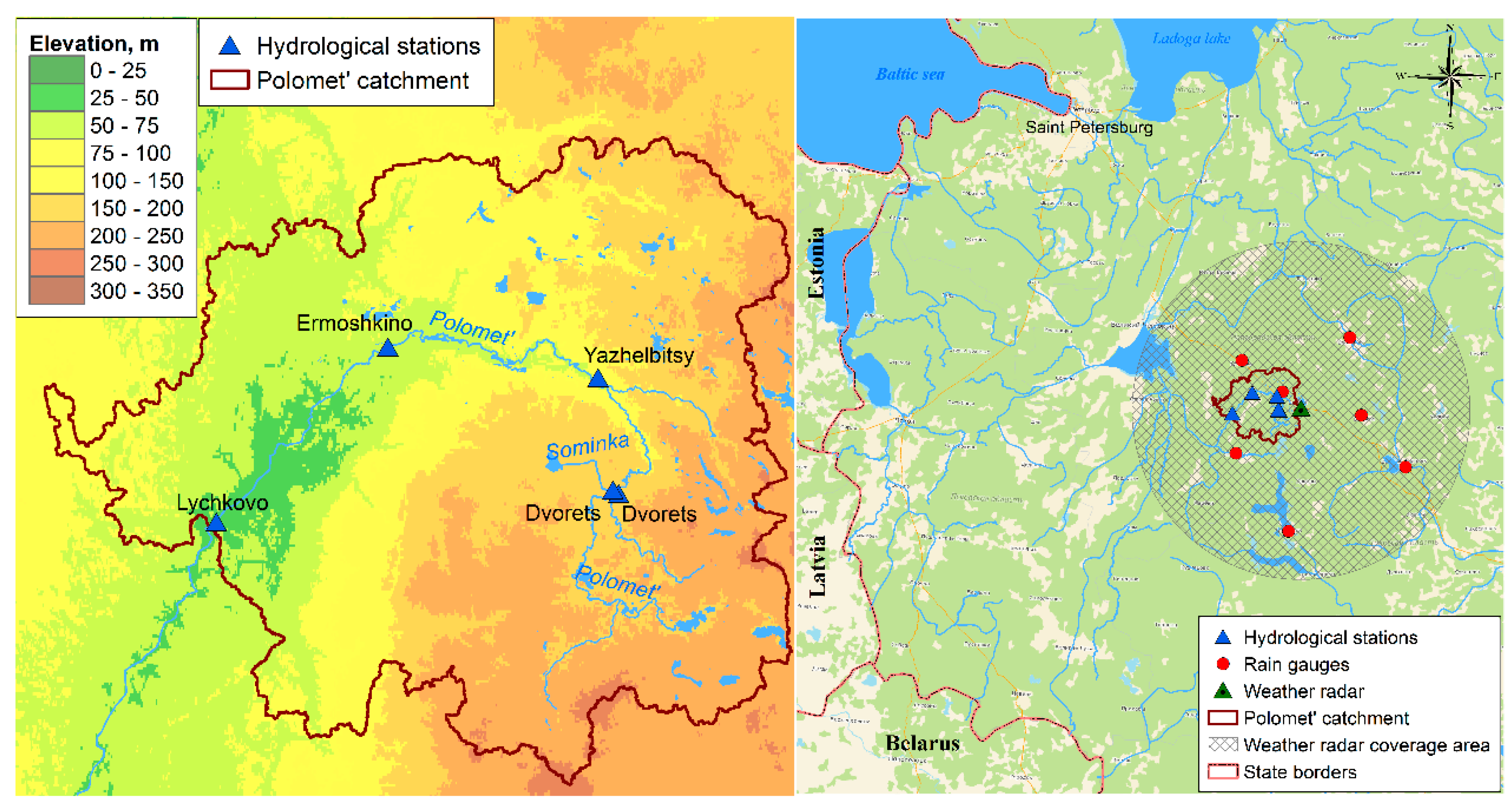
The area of this research is located in Novgorod region, Russia. The Polomet’ river, which is a key object of river runoff studies in this area, has been chosen as an object of investigation (Figure 1).

The Polomet’ river basin is located on the western slope of the Valdai Hills. The length of the Polomet’ river is 150 km, watershed is 2770 km². Relief and composition of quaternary deposits in the Polomet’ river basin is quite diverse. They were formed during the last glaciation under the influence of different processes associated with glacial retreat from the top and north-western proximal slope of Valdai Hills. The Polomet’ river basin is situated in temperate climatic zone. Local climate is influenced by both marine and continental air masses, frequent invasions of arctic masses, and active cyclonic processes. The main peculiarities of climate in this region are quite moist, warm winters, and long, quite cold winter seasons interrupted by frequent thaws.

Information on daily water discharge on the Polomet’ river have been used as the control hydrological information. The main attributes of investigated basins are summarized in

Table 1. Attributes of basins used for the modelling.

River	Gauge Station	Area (km2)	Stream Slope (‰)
Sominka	Dvorets	32.3	2.27
Polomet’	Dvorets	432	1.20
Polomet’	Yazhelbitsy	631	2.21
Polomet’	Ermoshkino	1180	1.53
Polomet’	Lychkovo	2180	1.36

.

2.2. Rainfall Data and Data Period

We have used 2 datasets for precipitation—from rain gauge and weather radar. Observations from manual rain gauges from the Russian Service for Hydrometeorology and Environmental Monitoring (Roshydromet) were only available with 24-h resolution. Temporal resolution of the radar used in this study is 10 min, aggregated to 1 day (equivalent to the temporal resolution of the rain gauge data) and spatial resolution 2 × 2 km. Figure 1 shows the location of the catchment within the utilized radar pixels. We use a summer period of 4 months from 1 June 2017 until 31 October 2017 for modelling rainfall runoff with different rainfall inputs.

2.3. Rainfall Radar Adjustment

In the adjustment, the rain gauges marked in Figure 1 are used. The adjustment is performed with only 6 rain gauges distributed in the study area.

The coefficients in the reflectivity (Z)–rain intensity (R) relationship are adjusted for the whole data period (summer period). The rainfall depths from all rain events at all considered rain gauges are plotted against the rainfall depths derived from the radar observations in the corresponding pixels. The Z–R coefficients are adjusted, such that the regression line between radar rainfall depths and rain gauge observations has slope 1). The resulting Z–R relationship is used for deriving rainfall depth over the whole data period.

$$Z=A \times R^b$$

(1)

where the coefficients A and b can be obtained by fitting the relation to match at least two points identified by non-zero concurrent measurements of rainfall rate and radar reflectivity.

Correction of Radar-Derived Data by Rain Gauges Data

Measurements at meteorological stations provide accurate information, but their density is insufficient to simulate rain floods caused by rainfall. While the coverage area of a meteorological radar covers large areas, however, this advantage over ground measurements is accompanied by significant errors.

Previous studies were aimed at comparing radar and ground-based precipitation data and indicated the existence of some bias in the radar precipitation estimates. Skinner et al. [19] showed an overestimation of small precipitation rates and underestimation of high precipitation rates by radar data. Borga et al. [20] showed a clear downward shift in the values of meteorological radar measurements compared to measurements at meteorological stations. All this points to the need to identify and account for such bias before using radar data in hydrological analysis.

There are many methods for combining radar and ground-based precipitation measurements. In this work, the residual interpolation method is used (using TIN geoprocessing tool). The essence of the method lies in the spatial interpolation of the difference between ground-based and radar measurements of the amount of precipitation for each period at the locations of meteorological stations. This difference is then computed using spatial interpolation for each representative point used for modeling. Then, the difference is subtracted or added to the values of the radar measurements. Thus, the amount of precipitation received by the radar method is being adjusted.

2.4. Modeling Procedures

The SWAT model could be used for both single basin modeling and system of multiple hydrologically-connected river basins. Each basin is firstly divided into various sub-basins (primary basins), which are in turn divided into hydrological response units (HRUs). HRUs are characterized by quite similar land use conditions, plant cover, relief characteristics, and soil cover. SWAT is a model with temporal averaging interval of 24 h. The model is physically justified and based on existing GIS-technologies [21].

The physical base of the SWAT model is the equation of water balance:

$$S{W}_t= S{W}_0+{\displaystyle \sum }_{i=1}^t\left(R_{day}-Q_{surf}-E_a-w_{seep}-Q_{gw}\right) ,$$

(2)

where i—model step (day, from 1 to t), SW_t—moisture content in soil at the end of calculation period i = t, mm; SW₀—initial moisture content in soil in the beginning of calculation period, mm; R_day—daily precipitation rate, mm; Q_surf—surface runoff, mm; E_a—evapotranspiration, mm; w_seep—quantity of water, saturated into the aeration zone through the soil profile; mm; Q_w—subsurface runoff, mm.

The structural base for the modeling and databases of landscape parameters were prepared using the ArcSWAT 2012 GIS interface for ESRI ArcGIS 10.4.1, the digital terrain model with the resolution of 90 × 90 m.

The data on land cover and land use as well as the vegetation cover have been taken from the open-source OpenStreetMap. All the missing information have been added manually using satellite imagery. We have used the national atlas for soils of Russia as a base for delineation of predominant soils in the area of study. The database of hydrological properties of soils was formed using the data from the literature sources [22]. The values of most of the parameters obtained during the literature review were clarified during the model calibration and were unified for the whole basin.

Potential evaporation was computed by the Hargreaves method, and channel transformation was calculated by the Muskingum method.

Daily rates of the below-listed characteristics at 2 meteorological stations (Valdai, Demyansk) during the period from 1994 to 2018 were used as the input data for modelling:

• Daily precipitation;
• Daily relative humidity;
• Daily maximal and minimal air temperature;
• Daily wind speed.

The hydrological regime for the Polomet’ River basin is simulated with a daily resolution for the period of 1994–2018 (25 years). Within the period mentioned has been also detected a calibration period (1994–2013) and verification period (after 2014). Since the Sominka river has a short series of observations—only 6 years (from 2013 to 2018)—the parameters were not calibrated. The river basin is a subbasin of Polomet’ (Yazhelbitsy) catchment and verification was carried out according to the parameters of this catchment.

SWAT modeling procedure includes numerous equations (equations of surface, subsurface, and groundwater runoff and from the equations of snow formation and melt) with undefined parameters, which could significantly affect the performance. Therefore, the main parameters affecting the modeling results have been determined (

Table 2. SWAT model parameters significantly affecting the model performance.

Parameter	Sominka	Polomet’	Polomet’	Polomet’	Polomet’
	(Dvorets)	(Dvorets)	(Yazhelbitsy)	(Ermoshkino)	(Lychkovo)
Sftmp (°C)	−0.095	−0.09	−0.09	−0.2	−0.75
Smtmp (°C)	4.7	4.7	4.7	4.7	4.7
CN2	35	40	35	40	40
Revapmn (mm)	137	137	137	137	137
Gw_Delay	1	1	1	1.5	3
Rchrg_Dp	0.55	0.6	0.55	0.55	0.6
Alpha_Bf	0.17	0.17	0.17	0.11	0.11
Gwqmn (mm)	47	47	47	47	47

). All of them were calibrated using the processing tools from ArcSWAT program.

At the first step, parameters that are common for the whole river basin were determined, such as Sftmp and Smtmp (snowfall and snow melt base temperature). The initial values of the moisture condition II (normal wetting) curve number (CN2) were determined for each soil type according to the description of their hydrological regime.

The value of threshold depth of water in the shallow aquifer (Revapmn) was calculated from the data on discontinuous capillary moisture for the lower soil horizons. For determination of the delay time for aquifer recharge (Gw_Delay), the assumption was made that most of precipitation from intense rains should be spent for subsurface and surface runoff. The initial value of the baseflow recession were constant for soil types (Alpha_Bf). The threshold groundwater level (Gwqmn), at which the return flow might occur, was pre-described according to the suggestions from Neitsch et al. [23] and determined during the model calibration.

Comparison of calculated and observed modelling runoff hydrographs has been performed using different approaches:

(i) Estimation of modelling quality during each year of calculation has been performed using the Nash–Sutcliff quality criteria (NSE), (ii) determination coefficient, and (iii) with comparing average water discharge rates. NSE criterion is calculated according to the equation below [24]:

$$NSE=1- \frac{{{\displaystyle \sum }}_{i=1}^n{\left(Q_i-P_i\right)}^2}{{{\displaystyle \sum }}_{i=1}^n{\left(Q_i-\overline{Q}\right)}^2}$$

(3)

where $Q_i$—observed water discharge during the i-time interval (m³ s⁻¹); $P_i$—calculated water discharge during the i-time interval (m³ s⁻¹); $\overline{Q}$—averaged observed water discharge during the whole period of modelling (m³ s⁻¹); $n$—the length of modelling period (years).

The criteria values are generally ranged between from −∞ to 1. In most cases, modelling is concluded as with good results when $NSE$ > 0.50 [25].

3. Results and Discussion

3.1. Runoff Modelling Using Rain Gauge Data

For the entire simulation period the average NSE value was 0.63 for all posts (

Table 3. Assessment of modelling quality for the whole period using rain gauge data.

River	Gauge Station	NSE	R2	Qob, m3 s−1	Qswat, m3 s−1
Sominka	Dvorets	0.57	0.62	0.37	0.37
Polomet’	Dvorets	0.60	0.72	5.11	3.86
Polomet’	Yazhelbitsy	0.71	0.72	7.12	6.06
Polomet’	Ermoshkino	0.62	0.73	14.2	11.4
Polomet’	Lychkovo	0.70	0.75	22.1	20.8

). The low values of NSE coefficient for all stations in 1994 (the first year of model simulation) is explained by the errors in setting the initial conditions for modeling (first of all, by the size of the liquid water layer in the calculated soil layer), the so-called “spin-up” of the model. To minimize the influence of the initial conditions during the model “spin-up” on the quality of model simulation, data from 1994 has been removed from the discussion.

The greatest discrepancy between the observed and simulated flow is observed during the winter and summer low water periods. Additionally, the decrease in the quality of modeling is associated with the inability of the model to capture winter thaws accurately.

In the first case, the most likely reason for such discrepancies is insufficient data on the distribution of heights and water reserves in the snow cover in different parts of the catchment, especially in the upland part. In the second case, the source of errors is the lack of data on the characteristics of groundwater: the rate and time of their discharge, and their contribution of underground layers to the river feeding.

Analysis of the observed and simulated average annual water discharges made it possible to establish that, not in all cases, the high NSE criteria correspond to small errors in the calculations of the runoff for individual years.

Table A1. Modelling quality criteria for the Polomet’ river—Dvorets station using rain gauge data.

Year	Qob, m3 s−1	Qswat, m3 s−1	Error, %	NSE
1994	4.91	0.37	92.55	−0.20
1995	5.83	3.01	48.35	0.53
1996	2.54	2.12	16.66	0.59
1997	4.55	3.73	17.94	0.78
1998	6.10	5.73	5.97	0.74
1999	4.17	3.24	22.32	0.26
2000	5.49	3.67	33.19	0.75
2001	3.92	3.20	18.45	0.81
2002	3.38	2.88	14.86	0.70
2003	5.66	3.07	45.72	0.59
2004	6.63	5.81	12.39	0.30
2005	5.25	4.08	22.17	0.63
2011	6.93	5.04	27.37	0.65
2012	5.68	3.49	38.56	0.64
2013	4.48	4.72	−5.35	0.85
2014	6.30	2.44	61.27	−0.20
2016	4.71	3.56	24.43	0.77
2017	7.9	6.7	−14.51	0.69
2018	2.48	2.97	19.57	0.84

,

Table A2. Modelling quality criteria for the Polomet’ river—Yazhelbitsy station using rain gauge data.

Year	Qob, m3 s−1	Qswat, m3 s−1	Error, %	NSE
1994	8.29	0.22	97.38	−0.37
1995	7.31	4.68	36.05	0.75
1996	3.63	3.19	12.11	0.72
1997	7.06	5.36	24.15	0.83
1998	9.77	7.82	19.91	0.76
1999	7.00	4.96	29.1	0.37
2000	7.63	5.81	23.84	0.85
2001	6.10	4.8	21.35	0.83
2002	5.33	4.43	16.91	0.86
2003	7.73	5.20	32.7	0.71
2004	9.82	8.5	13.44	0.05
2005	7.09	6.38	10.04	0.71
2006	6.69	5.12	23.38	0.83
2007	7.36	5.5	25.35	0.55
2008	8.28	7.93	4.32	0.82
2009	9.04	7.89	12.75	0.78
2010	6.65	4.48	32.69	0.81
2011	8.81	7.51	14.69	0.82
2012	7.76	5.13	33.98	0.72
2013	7.6	9.26	−21.83	0.89
2014	5.46	4.25	22.23	0.39
2015	5.26	3.89	26.07	0.74
2016	6.94	5.88	15.25	0.66
2017	12.0	11.2	−6.07	0.66
2018	5.96	5.05	−15.17	0.89

,

Table A3. Modelling quality criteria for Sominka river—Dvorets station using rain gauge data.

Year	Qob, m3 s−1	Qswat, m3 s−1	Error, %	NSE
2013	0.35	0.44	−27.34	0.69
2014	0.27	0.24	9.75	0.33
2015	0.28	0.23	18.44	0.64
2016	0.42	0.34	20.04	0.39
2017	0.64	0.63	−1.50	0.58
2018	0.26	0.31	19.66	0.78

,

Table A4. Modelling quality criteria for the Polomet’ river—Ermoshkino station using rain gauge data.

Year	Qob, m3 s−1	Qswat, m3 s−1	Error, %	NSE
1994	14.8	1.34	91	−0.35
1995	14.8	8.75	41	0.53
1996	7.03	6.11	13.1	0.76
1997	13.8	11.0	20.3	0.79
1998	18.6	17.4	6.1	0.76
1999	11.1	9.26	16.3	0.35
2000	15.1	10.7	29.3	0.72
2001	11.2	9.30	16.7	0.65
2002	9.51	8.07	15.2	0.68
2003	16.2	8.81	45.6	0.54
2004	20.9	17.4	16.4	−0.01
2005	15.5	11.8	24.1	0.49
2006	12.6	10.3	17.9	0.69
2007	-	-	-	-
2008	-	-	-	-
2009	21.5	15.5	27.7	0.69
2010	15.6	9.78	37.3	0.67
2011	18.6	14.9	19.6	0.81
2012	12.8	10.3	19.4	0.86
2013	8.15	13.9	−71.1	0.35
2014	8.94	7.32	18.1	0.55
2015	10.1	6.82	32.2	0.71
2016	14.1	10.5	25.6	0.55
2017	24.7	20.5	−16.8	0.67
2018	13.0	9.63	−25.9	0.79

and

Table A5. Modelling quality criteria for the Polomet’ river—Lychkovo station using rain gauge data.

Year	Qob, m3 s−1	Qswat, m3 s−1	Error, %	NSE
1994	24.90	2.57	89.70	−0.36
1995	20.30	16.40	19.10	0.65
1996	11.00	11.00	0.20	0.81
1997	20.70	19.10	7.50	0.81
1998	24.30	29.70	−22.00	0.63
1999	22.00	17.80	19.00	0.72
2000	26.50	19.70	25.90	0.76
2001	20.40	17.30	15.10	0.78
2002	15.90	15.40	2.70	0.73
2003	24.50	17.50	28.70	0.67
2004	31.70	30.80	2.90	0.44
2005	28.70	23.20	19.40	0.51
2006	21.70	17.40	19.60	0.70
2007	17.60	21.70	−23.10	0.72
2008	21.60	27.60	−27.80	0.60
2009	26.20	29.00	−10.50	0.65
2010	19.70	16.80	14.50	0.84
2011	23.90	26.20	−9.60	0.80
2012	24.30	19.60	19.30	0.72
2013	19.40	24.00	−24.10	0.80
2014	15.40	12.90	15.90	0.46
2015	13.20	10.20	22.80	0.85
2016	24.40	18.10	25.60	0.35
2017	34.70	37.00	6.70	0.70
2018	19.00	18.60	−2.30	0.80

show the values of the modeling results errors, from which it can be seen that the average annual water discharges (observed and simulated) have similar values, while the Nash–Sutcliff coefficient might be low or even negative. Unsatisfactory values were obtained in cases where there was a discrepancy between the peak and the volume of flood period (i.e., Polomet’ river—Ermoshkino station, 2004).

For the entire modeling period for the catchment Polomet’ (Dvorets), there is an underestimated value of the average annual water discharge, on average by 20%, in some years up to 60% in 2014. The reason for this may be an error in calculating the catchment area, as well as the lack of meteorological data in the upland part of the Polomet’ river basin.

Lower NSE values were noted at all stations of Polomet’ river basin in 2016. The reason for this may be the absence of reproduction of rain floods in July–August due to the passage of local precipitation in the basin area, which were not recorded at the nearest meteorological stations.

The errors in modeling rain floods are due to the unrepresentativeness of meteorological data for the catchment area of Polomet’ river in summer, as the SWAT model correlates weather stations with the center of each catchment on the basis of the nearest neighborhood. The observational network in the area of the study are quite scarce, which also applies for other regions of Russia [26]. This results in overestimation or underestimation of the actual amount of precipitation by scarce observation network of the investigated area. The unrepresentative nature of the meteorological station ‘Valdai’ is explained by its location outside the catchment of Polomet’ river (the station is located in near-watershed zone, which is characterized by high spatial variability of summer precipitation). Simulations using data from only two meteorological stations (Valdai and Demyansk) showed the need for a more accurate account of the spatial heterogeneity of the precipitation field. Such accounting is possible when using radar information.

According to previous studies by Santhi et al. [27] and Moriasi et al. [25], calibration and validation of modeling have good performances in case of NSE > 0.5. In general, the SWAT model captures well the different phases of the water regime and demonstrates a good quality of reproduction of the runoff hydrographs of the Polomet’ river (Table 3).

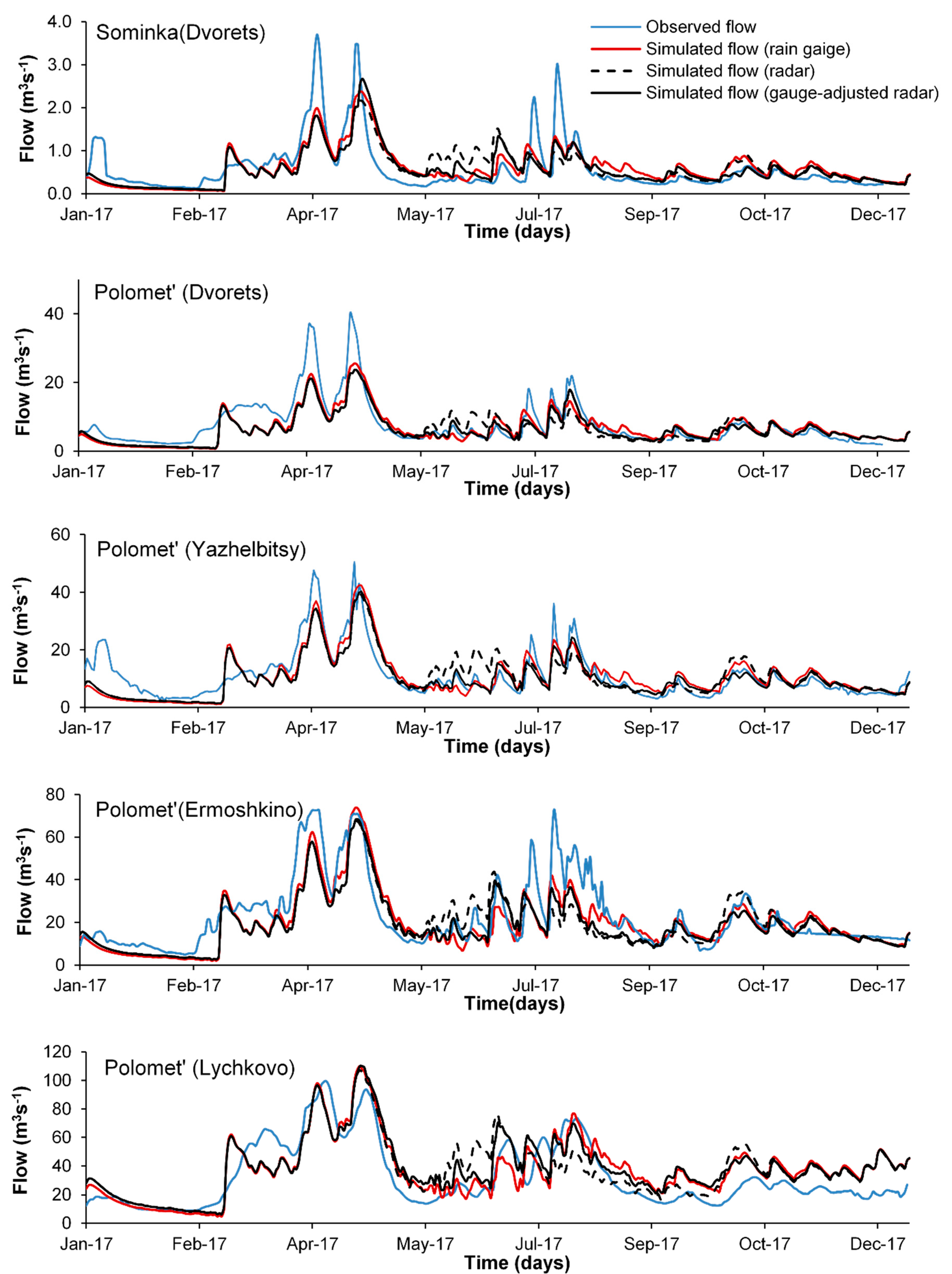
The results of runoff modelling for all the investigated gauge stations are shown in Figure 2.

3.2. Runoff Modelling Using Radar Data

Despite the fact that the Doppler weather radar “Valdai” has been operating since 2012, simulations for our study were only made for 2017. This is due to the fact that, from 2012 to 2016, the radars were periodically adjusted and had gaps up to 2 weeks due to the disconnection of the locator. No significant floods were observed in 2018.

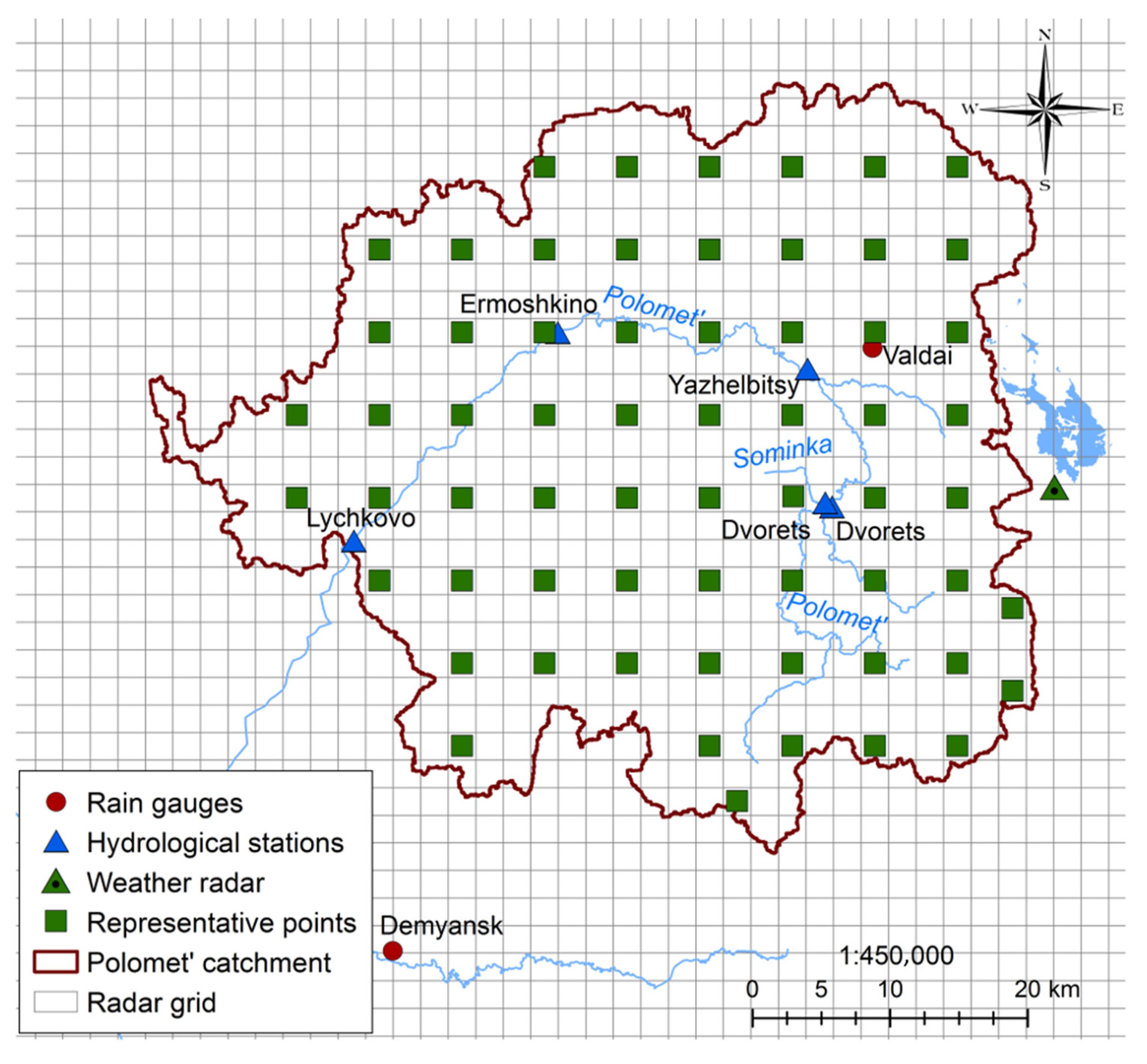
Interpolated rainfall data were used to “spin-up” the model and minimize the influence of the initial conditions for the simulation results. The catchment was represented by a 2 × 2 km radar grid (Figure 3). On the grid, 62 representative points were selected, information on reflectivity was averaged to a size of 4 × 4 km and was subsequently used for modeling.

The following information was used for modeling:

(1)

Daily data of the “Valdai” Doppler radar only for the warm period of the year, including the months from May to October;

(2)

Daily maximal and minimal air temperature, relative humidity, and wind speed of weather stations Demyansk, Valdai;

(3)

Interpolation data on atmospheric precipitation obtained at the weather stations Demyansk and Valdai for “spinning-up” the model.

Figure 2 shows the result of a runoff simulation for 2017 using radar data. Visual analysis showed that the model is sensitive to new information. Therefore, on the simulated runoff hydrographs, a series of summer-autumn floods can be clearly traced. However, in June, the water discharges calculated by the radar were overestimated by almost two times in comparison with the observed ones. At the same time, a number of floods in June, when using data from meteorological stations, were underestimated or missed due to the low amount of precipitation recorded by meteorological stations. In both cases, long-term floods caused by massive precipitation covering the entire basin from October to December are well reproduced.

Due to the strong discrepancy between the water discharge in June, the NSE value decreased due to the addition of new information.

3.3. Runoff Modelling Using Gauge-Adjusted Radar Data

Figure 2 shows the results of runoff modeling for 2017 using gauge-adjusted radar data. Visual analysis showed that, when combining the data, the model better reproduces a series of summer-autumn floods. However, the water discharge of the floods that took place in August was greatly underestimated or, as at Polomet’ river-Ermoshkino station, no floods were observed. The decrease in peak simulated values compared to measured ones in case of intense precipitation is also usually observed on the hydrographs (Figure 2). This coincides with results of previous studies aiming at runoff modeling in Far-East of Russia [28,29].

The NSE value has increased due to the addition of adjusted information compared to the modeling results based on only radar information. However, it turned out to be slightly lower than the modeling results using data from meteorological stations, except for Polomet’ river-Yazhelbitsy station (

Table 4. Modelling performance (NSE) using different input data.

Input Data	Sominka	Polomet’	Polomet’	Polomet’	Polomet’
	(Dvorets)	(Dvorets)	(Yazhelbitsy)	(Ermoshkino)	(Lychkovo)
Rain gauges	0.58	0.69	0.66	0.67	0.70
Weather radar	0.45	0.60	0.59	0.51	0.60
Gauge-adjusted radar	0.51	0.67	0.68	0.60	0.67

).

The choice of the calibration period for the ZR-relationship parameters, as well as the parameters themselves, also affect the simulation results. In our work, the selection of parameters was carried out for a long period from May to October due to the lack of more detailed information on atmospheric precipitation, such as data of urgent observations, information on the type of precipitation or data from rain gauges. Another reason may be an insufficient period for calibration and verification of SWAT model parameters.

Moreover, it is worth mentioning that the calibration of watershed models (i.e., SWAT) is subjective, since analyst knowledge of investigated watershed could not be replaced by any automatic calibration [30]. It was also shown previously that calibration of models should be based on the type and temporal resolution of data used [31,32].

4. Conclusions

The adaptation of the SWAT model to the conditions of flow formation in the Polomet’ river basin (north-west Russia) has been carried out. In general, the model captures different phases of the water regime well and demonstrates a satisfactory quality of reproduction of the Polomet’ river runoff hydrographs. It was revealed that the SWAT model can be used to simulate river flow, including rain floods.

The quality of modeling of rainfall floods was assessed using various types of information on atmospheric precipitation, including data from the Doppler Weather Radar. In general, the best model performance was observed for rain gauge data (NSE coefficient is up to 0.70 in the Polomet’ river-Lychkovo station); however, good results have been also obtained when using adjusted data. The discrepancies between observed and simulated water flows in the model might be explained by the scarce network of meteorological stations in the area of the studied basin, which does not allow for a more accurate correction of the radar data.

It was shown that the simulation results are highly dependent on the calibration period as well as various input parameters. Commonly, all the methods of calibration are based on a reverse simulation approach, which is connected with an inability to directly measure most of the input parameters required by the model. The main drawback of this method is the multiplicity of solutions, which is due to the presence of different sets of parameters that satisfy the given value of the objective function. To minimize this problem, there is a need for in-situ measurements.

The results of our study showed the necessity of selecting the appropriate radar and rain gauge observation strategies depending on the purpose of modelling. Hence, further research is needed to improve the effectiveness of radar data use for rainfall runoff modelling.

References

- The Siberian Times. Available online: https://siberiantimes.com/other/others/news/flood-apocalypse-in-eastern-siberia-kills-five-and-maroons-9919-whose-homes-destroyed-or-damaged (accessed on 20 August 2020).
- GISmeteo News. Available online: https://www.gismeteo.com/news/elemental-phenomena/32553-27-settlements-remain-flooded-in-novgorod-region (accessed on 20 August 2020).
- Sivasubramaniam, K.; Alfredsen, K.; Rinde, T.; Sæther, B. Can model-based data products replace gauge data as input to the hydrological model? Hydrol. Res. 2020, 51, 188–201. [Google Scholar] [CrossRef]
- Beven, K.J. Rainfall-Runoff Modelling; John Wiley & Sons Ltd.: Chichester, UK, 2020. [Google Scholar]
- Førland, P.; Allerup, B.; Dahlström, E.; Elomaa, T.; Jónsson, H.; Madsen, J.; Perälä, P.; Rissanen, H.; Vedin, F.; Vejen, F. Manual for Operational Correction of Nordic Precipitation Data. DNMI Rep. 1996, 24, 66. [Google Scholar]
- Taskinen, A.; Söderholm, K. Operational Correction of Daily Precipitation Measurements in Finland. Boreal Environ. Res. 2016, 21, 1–24. [Google Scholar]
- Montesarchio, V.; Orlando, D.; Del Bove, D.; Napolitano, F.; Magnaldi, S. Evaluation of optimal rain gauge network density for rainfall-runoff modelling. In AIP Conference Proceedings; AIP Publishing: Melville, NY, USA, 2015; Volume 1648, p. 190004. [Google Scholar]
- Noh, H.; Lee, J.; Kang, N.; Lee, D.; Kim, H.S.; Kim, S. Long-Term Simulation of Daily Streamflow Using Radar Rainfall and the SWAT Model: A Case Study of the Gamcheon Basin of the Nakdong River, Korea. Adv. Meteorol. 2016, 2016, 1–12. [Google Scholar] [CrossRef]
- Bell, V.A.; Moore, R.J. A grid-based distributed flood forecasting model for use with weather radar data: Part 2. Case studies. Hydrol. Earth Syst. Sci. 1998, 2, 283–298. [Google Scholar] [CrossRef] [Green Version]
- Choi, J.; Olivera, F.; Socolofsky, S.A. Storm Identification and Tracking Algorithm for Modeling of Rainfall Fields Using 1-h NEXRAD Rainfall Data in Texas. J. Hydrol. Eng. 2009, 14, 721–730. [Google Scholar] [CrossRef] [Green Version]
- Fares, A.; Awal, R.; Michaud, J.; Chu, P.-S.; Fares, S.; Kodama, K.; Rosener, M. Rainfall-runoff modeling in a flashy tropical watershed using the distributed HL-RDHM model. J. Hydrol. 2014, 519, 3436–3447. [Google Scholar] [CrossRef] [Green Version]
- Wyss, J.; Williams, E.R.; Bras, R.L. Hydrologic modeling Of New England river basins using radar rainfall data. J. Geophys. Res. Space Phys. 1990, 95, 2143–2152. [Google Scholar] [CrossRef]
- Smith, M.B.; Seo, D.-J.; Koren, V.I.; Reed, S.M.; Zhang, Z.; Duan, Q.; Moreda, F.; Cong, S. The distributed model intercomparison project (DMIP): Motivation and experiment design. J. Hydrol. 2004, 298, 4–26. [Google Scholar] [CrossRef]
- Smith, J.A.; Seo, D.J.; Baeck, M.L.; Hudlow, M.D. An Intercomparison Study of NEXRAD Precipitation Estimates. Water Resour. Res. 1996, 32, 2035–2045. [Google Scholar] [CrossRef]
- Ajami, N.K.; Gupta, H.; Wagener, T.; Sorooshian, S. Calibration of a semi-distributed hydrologic model for streamflow estimation along a river system. J. Hydrol. 2004, 298, 112–135. [Google Scholar] [CrossRef] [Green Version]
- Bandaragoda, C.; Tarboton, D.G.; Woods, R. Application of TOPNET in the distributed model intercomparison project. J. Hydrol. 2004, 298, 178–201. [Google Scholar] [CrossRef]
- Carpenter, T.M.; Georgakakos, K.P. Continuous streamflow simulation with the HRCDHM distributed hydrologic model. J. Hydrol. 2004, 298, 61–79. [Google Scholar] [CrossRef]
- Löwe, R.; Thorndahl, S.; Mikkelsen, P.S.; Rasmussen, M.R.; Madsen, H. Probabilistic online runoff forecasting for urban catchments using inputs from rain gauges as well as statically and dynamically adjusted weather radar. J. Hydrol. 2014, 512, 397–407. [Google Scholar] [CrossRef]
- Skinner, C.; Bloetscher, F.; Pathak, C. Comparison of NEXRAD and Rain Gauge Precipitation Measurements in South Florida. J. Hydrol. Eng. 2009, 14, 248–260. [Google Scholar] [CrossRef]
- Borga, M.; Anagnostou, E.; Krajewski, W. Validation of a Method for Vertical Profile of Reflectivity Identification through Bright Band Simulation. In Proceedings of the III International Symposium on Hydrological Applications of Weather Radar, Sao Paolo, Brazil, 20–23 August 1995; pp. 331–343. [Google Scholar]
- Winchell, M.; Srinivasan, R.; Luzio, M.D.; Arnolds, J.G. Arcswat Interface For SWAT2012. User’s Guide; Blackland Research and Extension Center, ARS Temple: Temple, TX, USA, 2013. [Google Scholar]
- Kapotova, N.A.; Kapotov, N.I. Investigation of water-physical characteristics of soils of non-Chernozem area of Russian part of the Soviet Union. In Trudy of State Hydrological Institute; Kapotova, N., Livanova, N., Eds.; Gidrometeoizdat: Leningrad, Russia, 1983; pp. 50–57. (In Russian) [Google Scholar]
- Neitsch, S.L.; Arnold, J.; Kiniry, J.; Williams, J. Soil and Water Assessment Tool Theoretical Documentation, Version 2009; Texas A&M Univ.: College Station, TX, USA, 2011. [Google Scholar]
- Nash, J.E.; Sutcliffe, J.V. River Flow forecasting through conceptual models-Part I: A discussion of principles. J. Hydrol. 1970, 10, 282–290. [Google Scholar] [CrossRef]
- Moriasi, D.N.; Arnold, J.G.; Van Liew, M.W.; Bingner, R.L.; Harmel, R.D.; Veith, T.L. Model Evaluation Guidelines for Systematic Quantification of Accuracy in Watershed Simulations. Trans. ASABE 2007, 50, 885–900. [Google Scholar] [CrossRef]
- Terskii, P.N.; Kuleshovm, A.A.; Chalovm, S.R. Water Balance Assessment Using Swat Model. Case Study on Russian Subcatchment of Western Dvina River. In Climate Change Impacts on Hydrological Processes and Sediment Dynamics: Measurement, Modelling and Management; Chalov, S., Golosov, V., Li, R., Tsyplenkov, A., Eds.; Springer Proceedings in Earth and Environmental Sciences; Springer: Cham, Switzerland, 2019; pp. 83–87. [Google Scholar] [CrossRef]
- Santhi, C.; Arnold, J.G.; Williams, J.R.; Hauck, L.M.; Dugas, W.A. Application of a watershed model to evaluate management effects on point and nonpoint source pollution. Trans. ASAE 2001, 44, 1559–1570. [Google Scholar] [CrossRef]
- Bugaets, A.N.; Gartsman, B.; Tereshkina, A.A.; Gonchukov, L.V.; Bugaets, N.D.; Sidorenko, N.Y.; Pshenichnikova, N.F.; Krasnopeyev, S.M. Using the SWAT Model for Studying the Hydrological Regime of a Small River Basin (the Komarovka River, Primorsky Krai). Russ. Meteorol. Hydrol. 2018, 43, 323–331. [Google Scholar] [CrossRef]
- Gartsman, B.; Tegai, N.; Bloschl, G.; Parajka, J. Comparative Testing of Rainfall-runoff Models in Different Climate and Landscape Conditions of Austria and Russia. Geophys. Res. Abstr. 2008, 10, EGU2008-A-04602. [Google Scholar]
- Abbaspour, K.C.; Rouholahnejad, E.; Vaghefi, S.; Srinivasan, R.; Yang, H.; Kløve, B. A continental-scale hydrology and water quality model for Europe: Calibration and uncertainty of a high-resolution large-scale SWAT model. J. Hydrol. 2015, 524, 733–752. [Google Scholar] [CrossRef] [Green Version]
- Arnold, J.G.; Moriasi, D.N.; Gassman, P.W.; Abbaspour, K.C.; White, M.J.; Srinivasan, R.; Santhi, C.; Harmel, R.D.; Van Griensven, A.; Van Liew, M.W.; et al. SWAT: Model Use, Calibration, and Validation. Trans. ASABE 2012, 55, 1491–1508. [Google Scholar] [CrossRef]
- Abbaspour, K.C.; Johnson, C.A.; Van Genuchten, M.T. Estimating uncertain flow and transport parameters using a sequential uncertainty fitting procedure. Vadose Zone J. 2004, 3, 1340–1352. [Google Scholar] [CrossRef]
Figure 1.
Map of the study area with the locations of the Doppler weather radar (Valdai), its 125-km coverage (circle), the locations of the 6 manual rain gauges and 5 hydrological stations.
Figure 2.
Observed and simulated (using rain gauge, radar, and gauge-adjusted radar data) flow at the investigated stations in 2017.
Figure 3.
The scheme of Polomet’ river basin with radar grid.