Assessment of Climate Change Impacts on River Flow Regimes in the Upstream of Awash Basin, Ethiopia: Based on IPCC Fifth Assessment Report (AR5) Climate Change Scenarios

Abstract

The Awash River Basin is the most irrigated area in Ethiopia, which is facing critical water resources problems. The main objective of this study was to assess the impacts of climate change on river flows in the upper Awash Subbasin, Ethiopia, using the soil and water assessment tool (SWAT) hydrological model. The ensemble of two global climate models (CSIRO-Mk3-6-0 and MIROC-ESM-CHEM with RCP4.5 and RCP8.5) for climate data projections (the 2020s, 2050s, and 2080s) and historical climate data from 1981–2010 was considered. Bias-corrections were made for both the GCM data. SWAT model was calibrated and validated to simulate future hydrologic variables in response to changes in rainfall and temperature. The results showed that the projected climate change scenarios were an increase in rainfall for the period of the 2020s but reduced for the periods of 2050s and 2080s. The annual mean temperature increases, ranging from 0.5 to 0.9 °C under RCP4.5 and 0.6 to 1.2 °C under RCP8.5 for all time slices. In the 2020s, annual mean rainfall increases by 5.77% under RCP4.5 and 7.80% under RCP8.5, while in 2050s and 2080s time slices, rainfall decrements range from 3.31 to 9.87% under RCP4.5 and 6.80 to 16.22% under RCP8.5. The change in rainfall and temperature probably leads to increases in the annual streamflow by 5.79% for RCP4.5 and 7.20% for RCP8.5 in the 2020s, whereas decreases by 10.39% and 11.45% under RCP4.5; and 10.79% and −12.38% for RCP8.5 in 2050s and 2080s, respectively. Similarly, in the 2020s, an increment of annual runoff was 10.73% for RCP4.5 and 12.08% for RCP8.5. Runoff reduces by 12.03% and 4.12% under RCP4.5; and 12.65% and 5.31% under RCP8.5 in the 2050s and the 2080s, respectively. Overall, the results revealed that changes in rainfall and temperature would have significant impacts on the streamflow and surface runoff, causing a possible reduction in the total water availability in the subbasin. This study provides useful information for future water resource planning and management in the face of climate change in the upper Awash River basin.

1. Introduction

Global population growth and its respective demand, as well as climate change, put the water resources under pressure. It is estimated that by 2050, about 4.8 to 5.7 billion people will be living under potentially water-scarce areas. Africa is one of the most susceptible regions to climate change and variability [1]. Climate change is accelerating from time-to-time over the Earth’s surface due to the increase in human activities [2]. According to the Intergovernmental Panel on Climate Change [3], in comparison to earlier decades, radiative forcing on the natural system has increased a manifold from the 1970s. Accordingly, the total radiative forcing is reported to be 43% higher in IPCC Assessment Report 5 (AR5) than AR4 [3]. Global temperatures have shown an increase of around 0.74 °C during the last century (1906–2005), according to IPCC AR5 [3]. Thus, in all Representative Concentration Pathways (RCPs), a likely increase in the global warming trends during the twenty-first century has been well reported [4]. The change in both local and global climate, magnitude, and pattern of temperature and rainfall, affects the rate and occurrence of hydrologic processes such as water cycle and water resources. Water is a critical and vital resource for both human uses and ecosystem services [5,6,7,8]. Rivers are among the water resources important for their use in domestic, agricultural, and industrial purposes. The upper Awash River is the major water resource in the central rift valley, a subbasin that suffers from an increasing shortage of natural water resources. There is a tremendous increase in the demand for rivers; an increasing number of populations, advanced irrigation practices, and industrial usages are some of them [7,9].

The projected climate change will increase water scarcity risks at a peak level [10]. Climate changes also alter hydrological processes that maintain water supply and ecosystem function [11], and its impact is felt through changing patterns of water resources [12,13]. Moreover, an increase in temperature is hastening the global hydrologic cycle [14]. The hydrologic cycles that connect the lithosphere, atmosphere, and biosphere are most likely affected by global warming [15,16]. Almost all regions of the world have experienced global warming, with global air temperatures increasing by 0.85 °C, over the past half-century [1]. The variability and uncertainty of water resources associated with climate change are critical issues in arid and semi-arid regions of the world [9], and tropical river catchments face the challenges of the water resource as the population grows exponentially [17]. The impacts of climate change on hydrological variables and its processes have been studied extensively, particularly on surface runoff, groundwater flow, streamflow, and evapotranspiration, and soil moisture, by analyzing projected and downscaled climatic data and using different hydrological models [18,19,20,21,22,23,24,25]. This is particularly prominent in semi-arid and arid regions because in these regions, water resources, primarily streamflow and surface runoff, are highly sensitive to climate change; a small change in climate variables may result in significant variations of hydrological cycles and subsequence changes of regional water resources [26,27,28,29,30]. Thus, climate change and climate variability, the need for managing water resources require immediate attention and action.

Furthermore, climate change impact needs to be evaluated; at local and regional scales. This will require climate projection information at a spatial scale relevant to the system of interest, which is often significantly smaller than the resolution of GCMs, and thus, dynamic downscaling with RCMs is capable of addressing this scale gap [31]. In Ethiopia, a number of studies have been conducted to investigate the impacts of climate change on water resources by using hydrological models and several emission scenarios [32,33,34,35,36,37,38,39,40]. The reports revealed that climate, land use, and cover changes are among the main drivers of land degradation, which in turn largely affect water resources.

In the upper Awash Subbasin, water scarcity problems are becoming increasingly common due to higher water demand, urbanization, economic development and climatic variability [32,34,41,42]. Downstream irrigation and industrial enterprises in the upper Awash Sub-basin have been expanding from time to time with climate variability and leading to competition for water among different sectors coupled, thereby will pose a great problem on meeting the future water demands [32,41]. This necessitates the need for knowledge of future climate change and water resources availability taking into account. In that regard, a few studies have been reported in investigating climate change impacts on river flow, using RCPs emission scenarios in the basin. Thus, more information is necessary for a better plan of the adaptation strategies and water management practices under changing climate.

Climate models are important tools utilized to advance our understanding of the current and past climate [43]. However, despite all their complexity of our Earth imposes important limitations on existing climate models, and they represent simulations of the real world, constrained by their ability to correctly capture and reveal each of the important processes that operate to affect climate [43,44]. Similarly, global climate models attempt to describe the earth’s climate and are used in a variety of applications [45]. These include the study of the possible causes of climate change and the simulation of past and future climates, understand complex earth systems, and improving our understanding and predictability of climate behavior on seasonal, annual, decadal, and centennial time scales [45,46]. However, these models have several limitations, including an incomplete understanding of the climate system, an imperfect ability to transform our knowledge into accurate mathematical equations, the limited power of computers, the models’ ability to reproduce important atmospheric phenomena and inaccurate representations of the complex natural interconnections [45]. Downscaling is required because of the limitations of coarse spatial resolution in the global models [44]. Thus, downscaling improves some aspects of the performance of models and their ability to represent observations; this technique is still subject to the general limitations suffered by all numerical models [43].

Here we propose a methodology that uses the output of two ensembles of bias-corrected global climate models (GCMs) as input to hydrological modeling and applies the outcome to the upper Awash River for predicting future runoff and streamflow. To address this, we evaluated climate change impacts on river flow using two ensemble GCMs under two RCPs emission scenarios. This effort essentially involves taking projections of climate at a regional scale and downscaling it at a regional-scale for all climatic variables considered, then finally downscaled to local scale and computing its impact on hydrological components using SWAT. The SWAT model is a useful tool for investigating climate change effects on water resources [47,48,49,50]. Its application was used in simulating surface runoff, streamflow, groundwater, and sediment transport, as well as the assessment of climate and land-use change impacts on the hydrology of river basins [25,27,51,52,53,54,55,56]. However, there are some of the limitations of this study that could be addressed in future research. The limitations and uncertainties are mainly related to the input data, the climate models and projections, the representation of physical processes and its algorithm in the hydrological model. The primary limitation to the generalization of these results is the use of only two ensembles GCMs and their spatial resolution that may lead to biases in the estimation of future climate and hydrology. Similarly, this analysis does not cover the effect of change in the magnitude (variability) of temperature/rainfall on the simulated streamflow. Another limitation presented in this study is linked to the land use and soil properties used in model development under current climate conditions were assumed to be constant and remain valid under conditions of future climate change. There is no consideration of changes in land use and soil properties in a simulation of future hydrology that may influence our model estimates. Thus, further research is recommended to address the limitations of this study for improved understanding and assessments that will prove useful for planning purposes in the upper Awash River Basin. This study provides insights on future trends of the subbasin response for the basin stakeholders to address water management issues.

The objective of this study was to evaluate the impacts of climate change on river flows in the upstream Awash Basin using the soil and water assessment tool (SWAT) model and ensemble global climate models (GCMs) under two RCPs emission scenarios.

2. Materials and Methods

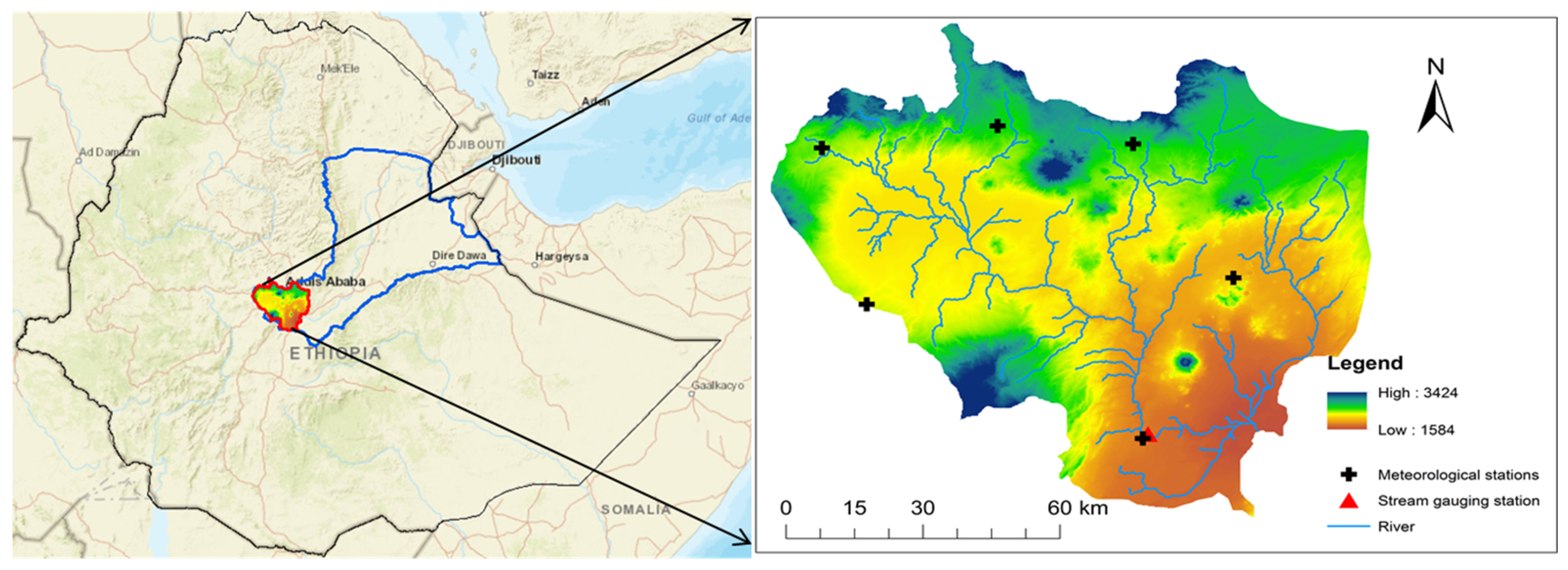
2.1. Description of the Study Area

The Awash Basin lies over the central highland of Ethiopia and has a drainage area of about 110 × 10³ km². This study was undertaken on the upper part of the Awash River Basin; located between 8°16′ and 9°18′ North latitude and between 37°57′ and 39°17′ East longitude (Figure 1). The Subbasin area covers a surface of about 7240 km².

The basin received an annual mean rainfall of 1019 mm through the period of 1980–2013. Mean maximum, minimum, and average values of temperatures recorded at the basin during the season were 12.10 °C, 23.20 °C, and 17.65 °C, respectively. The major soil groups identified by FAO are Vertisols, Luvisols, Cambisols, Nitisols, Andosols, Fluvisols, Regosols, and Leptosols. Vertisols are the dominant soils of the subbasin, covering about 40% of the total [57]. The report showed that the Vertisols are mainly distributed in the central highland plateau, including the surroundings of Addis Ababa areas, and these areas are characterized by intensive cultivation of teff and wheat. Moreover, Nitisols, Luvisols, and Cambisols cover about 27%; their distribution is mainly in the northern part, around Holeta and Sululta; and Nitisols and Luvisols are red soils that cover areas characterized by high rainfall [57]. About 80% of the Upper Awash River Basin is covered by Haplic Luvisoils and agricultural crops.

The main crops of the study area are wheat, teff (Eragrostis tef), barley beans, and other different types of grains and vegetables. Pasture lands, permanent open water bodies, and grassland associated with bushes and shrubs are also important units of land use/cover. Irrigated fields, swamps, and settlements cover a small area in the subbasin. About 68% of the total study area is flat or slightly undulating, with a slope between 2% and 8%. The annual runoff within the basin is estimated at 4.6 km³, and some tributaries like Mojo, Akaki, Kassam, Kebene, and Mile Rivers carry water the whole year while many lowland rivers only function during the rainy seasons [37].

In addition to the agricultural and purposes industrial, the Awash River used as a drinking water source for the city of Addis Ababa, Adama, and other rural towns within the basin [32,41].

2.2. Datasets

In the present study, the following geospatial data and hydro-climatic variables were used for analyses. The daily meteorological data, including rainfall, minimum and maximum temperature at six meteorological stations, were obtained from the National Meteorology Agency (NMA) of Ethiopia for the period (1981–2010). The daily observed streamflow data at the outlet of the basin covering the 1980–2010 periods were provided by the Ethiopian Ministry of Water Resources. The general information of selected meteorological stations is shown in

Table 1. General information of meteorological stations.

No	Station	Lat. (°N)	Lon. (°E)	Elev. (m)	Mean RF (mm)	Avg. Temp. (°C)
1	Addis Ababa	9.03	38.75	2354	1145.1	15.8
2	Debrazeit	8.73	38.95	1900	962.3	18.5
3	Holeta	9.07	38.48	2380	1048.96	15.5
4	Tulubolo	8.67	38.22	2100	1076.4	16.6
5	Ghinch	9.02	38.13	2132	1025.2	*
6	Hombole	8.37	38.77	1665	955.8	*

* Data not available (the station that has no temperature recording stations).

. An ensemble of the two global climate models (CSIRO-Mk3-6-0 and MIROC-ESM-CHEM with RCP4.5 and RCP8.5 emissions) was used to generate future climate projections at selected stations. The historical simulations were forced by observed data and anthropogenic atmospheric composition covering the period 1981–2010, whereas the projected one range from 2011 and 2100 derived via RCP4.5 and RCP8.5 emission scenarios. The simulated data of RCP4.5 and RCP8.5 scenarios were generated from CSIRO-Mk3-6-0 and MIROC-ESM-CHEM of the global climate model outputs.

The 90-m digital elevation model (DEM) (http://gdex.cr.usgs.gov/gdex/) was obtained from the shuttle-radar topographic mission (SRTM) for the delineation of the subbasin and to analyses the drainage systems on the study area. Subbasin components (slope length and slope gradient) and the stream network characteristics (channel width, length, and slope) were derived from this DEM.

The hydrological response units (HRUs) of the watershed were defined using soil and land use data. SWAT requires different physical, chemical, and soil textural properties such as available water content, soil texture, hydraulic conductivity, bulk density, and organic carbon content for different layers of each soil type. Soil physical and chemical properties databases from different studies in the basin were used. The infiltration and hydraulic conductivity of the major soils of the Awash Basin were measured and calculated [41,58]. All necessary soil information was obtained from the Awash River Basin Integrated Development Master Plan Project, Semi-detailed Soil Survey, and the Soil of Upper Awash area [57]. The land use/land cover map of the study area was obtained from the OWWDSE [57] and the Ministry of Water Resources of Ethiopia. They have reclassified the land use/land cover map of this area based on the available topographic map at a scale of 1:50,000, aerial photographs and satellite images.

2.3. Modeling Approach

Global climate models (GCMs) and regional climate models (RCMs) are important tools to assess climate change impacts. In this present study, changes in surface hydrology as a result of climate changes were assessed using the following procedure: (1) rainfall and temperature were considered and characterized for the baseline period. (2) The bias-corrected GCMs data using RCP4.5 and RCP8.5 were incorporated as an input to the SWAT model for the future time slices: 2020s, 2050s, and 2080s. A weather generator (WXGEN) model is included in SWAT, which can generate daily climate data. A weather generator WXPARM program reads daily values of maximum and minimum temperature, precipitation, solar radiation (calculated from daily sunshine hours), relative humidity, and wind speed data to calculate monthly averages and standard deviations of all the input variables.

Therefore, a weather generator was used to produce daily climate data to serve as input for the SWAT model to simulate streamflow and runoff.

2.3.1. Description of the Global Climate Model (GCM) and Climate Scenarios (RCPs)

The ensemble means of two climate models: CSIRO-Mk3-6-0 (resolution = 192 × 96 km²) and MIROC-ESM-CHEM (resolution = 128 × 64 km²) were selected based on their spatial resolution for the atmospheric variable (longitude*latitude) and their further applicability to African climate impact studies; and encouraged by its effectiveness in reproducing the climate in Ethiopia with respective RCPs [59,60,61,62,63], both with respect to other CMIP5 generation. Two different RCPs: RCP4.5 is having CO₂ concentration of 650 ppm equivalent with A1FI SRES of the third and fourth assessment report and RCP8.5 having CO₂ concentration of 1370 ppm equivalent with B1 SRES [64,65] were employed to downscale the rainfall, temperature (minimum and maximum) from GCMs to specific locations. The two RCPs were chosen to consider the impacts of CO₂ emitted to the atmosphere at medium and high emission concentrations.

2.3.2. Soil and Water Assessment Tool (SWAT) Model

SWAT is a physically-based semi-distributed and continuous-time hydrological model, with the most promising and computationally efficient capacity to operate on large basins in reasonable time [66]. SWAT was established to forecast the impact of land management practices on agricultural chemical yields of water and sediment in catchment basins with varying management conditions in soils and land use over long periods [67]. The model simulates 8 (eight) major components: agricultural management, soil temperature, hydrology, weather, crop growth, nutrients, pesticides, and sediment transport and erosion [68]. Major hydrological processes that can be simulated by the SWAT model include surface runoff, percolation, evapotranspiration (ET), infiltration, deep aquifer flows, and channel routing, and shallow aquifer [67]. The hydrological model was calibrated and verified using observed streamflow data of the subbasin. The model was selected because of its simplicity, availability, and widely acceptance [69].

Daily meteorological data of rainfall, solar radiation, minimum and maximum temperature, wind speed, and relative humidity were fed to the model. Data are given to the model as a user-defined observed time series and WXGEN model generated within SWAT from monthly data to filling the missing climate data [68].

Hence, simulation of basin hydrology with The SWAT model system embedded within a GIS, ArcSWAT, was undertaken in two isolated cases. The first case is the hydrological cycle given by the land phase, which controls the amount of pesticide, water, nutrient, and sediment loading to the main channel in each subbasin. The second case is a hydrologic cycle by routing phase, which can be defined as the movement of organic chemicals, water, nutrients and sediments load through the channel network of the catchment to the outlet. The model simulates the land phase hydrological cycle based on the water balance as given in Equation (1):

$$S{W}_t=S{W}_o+{\displaystyle \sum }_{t=1}^t\left(R_{day}-Q_{surf}-E_a-{\omega }_{sweep}-Q_{gw}\right)$$

(1)

where SW_t is the final soil water content (mm); SW_o is the initial soil water content (mm); t is the time (days); R_day is the amount of precipitation on day i (mm); Q_surf is the amount of surface runoff on day I (mm); E_a is the amount of evapotranspiration on day i (mm); ${\omega }_{sweep}$ is the amount of water entering the vadose zone from the soil profile on day i (mm), and Q_gw is the amount of return flow on day i (mm). Moreover, we employed the Green and Ampt infiltration method [70] and the Green and Ampt infiltration method [71] for estimating surface runoff through the SWAT model. It was explained that the SCS curve number procedure is a function of the soil’s permeability, antecedent soil water conditions and land use. SWAT model simulates surface runoff by using the SCS curve number method Equation (2).

$$Q_{surf}=\frac{{\left(R_{day}-I_a\right)}^2}{(R_{day}-I_a+S)}$$

(2)

where Q_surf is the accumulated runoff or rainfall excess (mm); R_day is the height of rainfall for day (mm); I_a is the initial abstractions (canopy interception, surface storage, infiltration prior to runoff) (mm) and S the retention parameter. Therefore, retention parameter S is defined as Equation (3):

$$S=25.4\left(\frac{1000}{CN}-10\right)$$

(3)

where CN is the curve number for day and the initial abstractions, I_a, are commonly approximated as 0.2S. Equation (4) is represented as follows:

$$Q_{surf}=\frac{{\left(R_{day}-0.2S\right)}^2}{\left(R_{day}+0.8S\right)}$$

(4)

Runoff will only occur when R_day > I_a.

2.4. Bias Correction Method

GCMs, provide climate data on a global scale. Thus, in order to assess the impact of changes in the climatic variables, such as precipitation and temperature, on water resource and hydrology systems, the outputs of GCMs need to be downscaled [72]. Downscaling is a process of obtaining high-resolution climate change or climate information from relatively coarse-resolution GCMs. The Local climate is influenced greatly by local topographies, such as mountains, which are not well-represented in GCMs because of their coarse resolution [73].

For hydrological simulations, raw data of RCPs were corrected using a linear scaling bias correction method [72,73]. In the bias correction method, transformation algorithms were used to adjust GCM’s climate variables. The approach was based on the determination of possible biases between measured and simulated climate variables and represents the starting point for correcting both control and the scenario RCM runs. Precipitation was corrected by fitting it to the long term (1981–2010) baseline data and measured for its coefficient of variation [74]. The temperature was corrected by fitting it to long term (1981–2010) baseline data and to the standard deviation (SD). We used a power transformation as an alternative by which corrects the average, as well as the CV [74]. In this nonlinear correction, each daily precipitation amount P is transformed into a corrected p* by using Equation (5) as follows:

$$P^{*}=a{P}^b$$

(5)

The coefficients a and b were iteratively determined. The mean coefficient b was determined by equating the CV of the observed value of precipitation with that estimated (GCMs) on a monthly basis, and the coefficient a was determined by equating the mean value of observed precipitation with that estimated for the basic period.

Temperature bias correction only involved scaling and shifting to adjust the mean and variance of GCMs and observed climate data [75,76]. The corrected daily temperature $T_{corr}$ was obtained by using the following Equation (6):

$$T_{corr}={\overline{T}}_{obs }+\frac{\sigma \left(T_{obs }\right)}{\sigma \left(T_{gcm }\right)}\left(T_{gcm}-{\overline{T}}_{obs}\right)+\left({\overline{T}}_{obs}-{\overline{T}}_{gcm}\right)$$

(6)

where $T_{corr}$is the corrected daily temperature; $T_{gcm }$ is the uncorrected daily temperature from the GCM model; $T_{obs }$ is observed daily temperature; ${\overline{T}}_{obs}$ and ${\overline{T}}_{gcm}$ are mean temperatures for observed and simulated GCM datasets, respectively.

2.5. Model Performance Evaluation

Sensitivity analysis was done on the SWAT model to select the best sensitive hydrological parameters. From the total of 27 hydrological parameters that are involved in the SWAT model for calibration, eight most sensitive parameters were selected (

Table 2. Hydrological parameters and their ranges used for model calibration.

No	Parameters	Description	Min	Max	Fitted Value
1	Alpha_Bf	Base flow recession	0.00	1	0.643
2	Cn2	Initial SCS CN II value	−0.25	0.25	0.496
3	Ch_K2	Channel effective hydraulic conductivity [mm/h]	0	150	136.680
4	Esco	Soil evaporation compensation factor	0	1	0.168
5	Sol_Z	Depth from the soil surface to bottom of the layer	−0.25	0.25	0.077
6	Ch_N2	Manning’s “n” value for the main channel	0	1	0.711
7	Blai	Maximum potential leaf area index	0	1	0.036
8	Revapmn	The threshold depth of water in the shallow aquifer for “revap” or percolation to the deep aquifer to occur	0	500	434.340

). A total of 27 parameters with ten intervals of LH sampling and 270 iterations were done to select the rank of these most sensitive parameters. Thus, each parameter was estimated after 1000 simulations (one iteration) until the performance criteria were satisfied. The most sensitive parameters to simulate streamflow were Alpha_Bf, Cn2, Ch_K2, Esco, Sol_Z, and Ch_N2. The curve number (CN2) was sensitive to discharge and peak flow. The CN2 value was calibrated within −25% to 25%; it was fitted at 4.96% that indicates discharge and peak flow, and baseflow recession constant (ALPHA_BF) was Varied 0 to 1 and calibrated at 0.643 values.

The SWAT model was manually and automatically calibrated and validated by using observed monthly gauged streamflow data at the Hombole outlet of the watershed. Validation verifies the performance of the SWAT model for simulated streamflows in different periods from the calibration periods without any additional tuning in the calibrated flows. Once calibrated and validated, the SWAT model was used for future predictions under different climate scenarios, if the SWAT model simulates reasonably in both the validation and calibration phases.

The performance of the SWAT model was assessed by using most statistical methods to define the reliability and quality of predictions when compared to measured values. For the goodness of fit measures, Nash–Sutcliffe simulation efficiency E_NS and coefficient of determination R₂ [77] was used to assess the SWAT model prediction. R² and E_NS values are explained in Equations (7) and (8), respectively.

$$R^2=\left[\frac{{{\displaystyle \sum }}_{i=i}^N\left(o_i-\overline{o}\right)\left(p_{i }-\overline{p}\right)}{\left[{{\displaystyle \sum }}_{i=1}^N{\left(o_{i }-\overline{o}\right)}^2\right]\left[{{\displaystyle \sum }}_{i=1}^N{\left(p_i-\overline{p}\right)}^{0.5}\right]}\right]$$

(7)

$$E_{NS}=1-\frac{{{\displaystyle \sum }}_{i=1}^N\left(o_i-p_i{)}^2\right)}{{{\displaystyle \sum }}_{i=1}^N{\left(o_i-\overline{o}\right)}^2}$$

(8)

where N is the number of compared values ∞, O_i is the observed data, $\overline{o}$ is the observed average, P_i is the simulated data and $\overline{p}$ is the simulated average. E_NS can have values ranging from −∞ to 1.

The ability of the hydrologic model to simulate streamflow was evaluated by computing Kling-Gupta efficiency (KGE), mean bias error (MBE), mean absolute error (MAE), and root-mean-square error (RMSE). The bias provides a measure of systematic errors revealed from comparing model results with measurements. The RMSE gives an estimate of the variability of the model compared with observation. Therefore, SWAT model performances were assessed in terms of goodness-of-fit performance (KGE, E_NS and R²) in order to assess the quality of the simulation in future hydrology under a change in the climate. KGE is given by:

$$KGE=1-\sqrt{{\left(CC-1\right)}^2+{\left(\frac{cd}{rd}-1\right)}^2{\left(\frac{cm}{rm}-1\right)}^2}$$

(9)

where CC is the Pearson’s coefficient value, and rm is the average of observed values and cm is the average of forecast values, and rd is the standard deviation of observation values, and cd is the standard deviation of forecast values.

The mean bias error (MBE) can indicate whether the model overestimates or underestimates the power output:

$$MBE=\frac{1}{n}{\displaystyle \sum }_{i=1}^n\left(p_i-o_i\right)$$

(10)

where $O_i$ the observation is value and $P_i$ is the forecast value.

In addition, the degree of accuracy of each model was evaluated using the root-mean-square error (RMSE) and mean absolute error (MAE), which is a good indicator to represent the quality of the model and its ability to describe the real behavior of each system. RMSE is given by:

$$RMSE=\sqrt{\frac{{{\displaystyle \sum }}_{i=1}^n{\left(X_{obs,i}-X_{model,i}\right)}^2}{n}}$$

(11)

where $X_{obs}$ is the observation value and $X_{model}$ is the model value.

Both RMSE and MAE express average model prediction error in units of the variable of interest. The RMSE and MAE can range from 0 to ∞ and are indifferent from the direction of errors. MAE is given by:

$$MAE=\frac{1}{n}x{\displaystyle \sum }_{i=1}^n\left|O_i-P_i\right|$$

(12)

where $O_i$ is the observation value, $P_i$ is the forecast value and |$O_i$ − $P_i$| = the absolute errors

2.6. Climate Change Impact Assessment

Detailed climate models and long hydrological records are needed to predict future conditions in a changing world [78]. The bias-corrected ensemble mean of GCMs data using RCP4.5 and RCP8.5 were given as an input to the SWAT model for the periods of 2020s, 2050s, and 2080s. The remaining climatic and all other land use and soil hydrologic properties used in model development under current climate conditions were assumed to be constant and remain valid under conditions of future climate change. There is no consideration of changes in land use, soil properties, and other climatic variables, which could influence the hydrology of the basin. The assumption of stationarity, which has been made so far in runoff and streamflow forecasts studies, is now being challenged. Such a study should not be considered as actual accurate scenarios because the latter would need to include future soil and land-use change impact. The model calculates the impacted daily precipitation by multiplying the daily precipitation multiplier by the corresponding baseline daily precipitation values; whereas the impacted daily temperatures were calculated by adding the average daily delta values of the maximum and minimum daily temperature to the corresponding average baseline daily temperature as shown in Equations (9) and (10).

$$R_{day}=R_{day}\times \left(1+\frac{ad{j}_{pcp}}{100}\right)$$

(13)

R_day is the precipitation falling in the subbasin on a given day (mm H₂O), and adj_pcp is the percentage change in rainfall.

$$T=T+ad{j}_{tmp}$$

(14)

T is the daily temperature (°C); adj_tmp is the change in temperature (°C).

To simulate the seasonal and annual changes under given climatic conditions, the monthly delta and precipitation multiplier values were used and applied evenly on all the days of the month. For the selected RCP4.5 and RCP8.5 climate change scenarios, the amounts of runoff and base flow as generated by the SWAT model were compared with those obtained from the baseline stream flow. In this work, the analyses were performed based on annual and three seasonal periods; kiremt (JJAS), Bega (ONDJ), and Belg (FMAM), and this helps to provide a seasonal comparison of changes in the climatic and hydrologic variables in the study area.

3. Results and Discussion

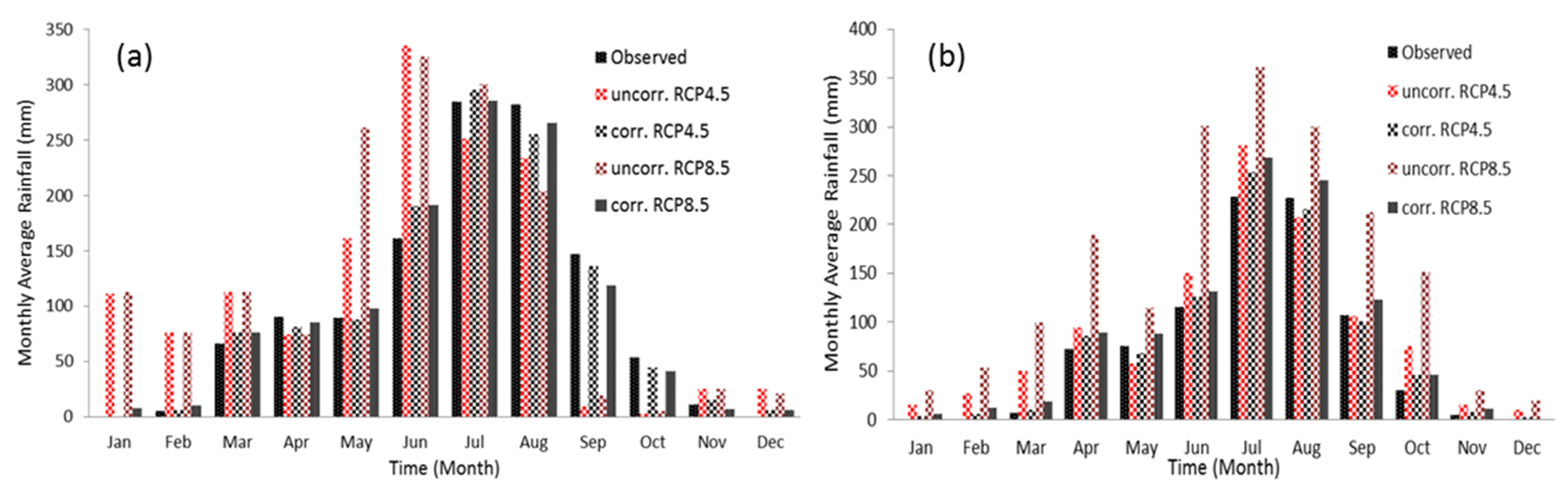
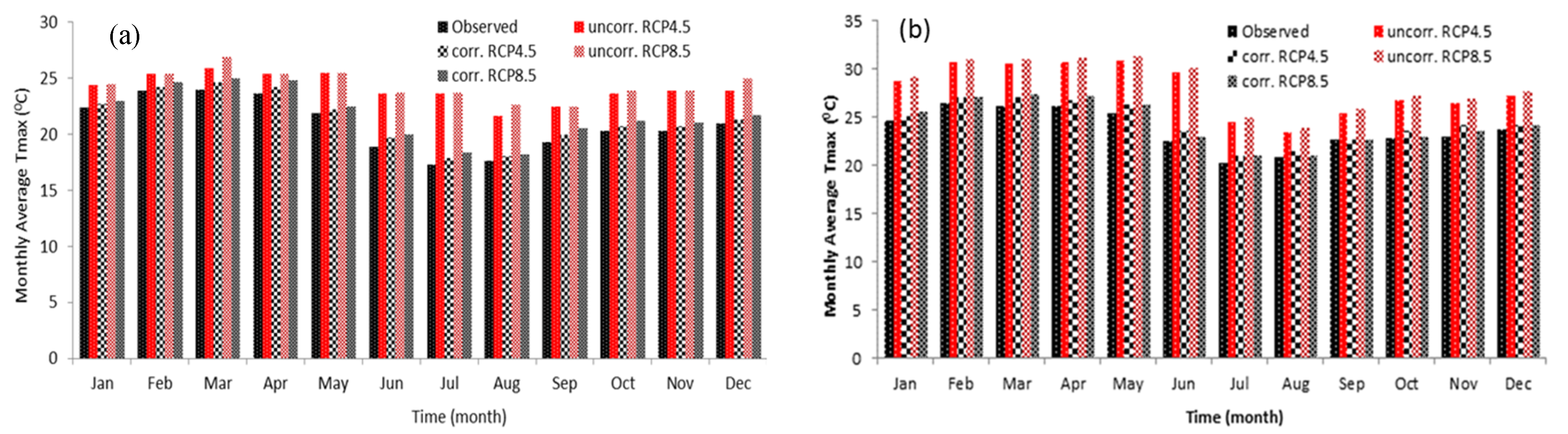
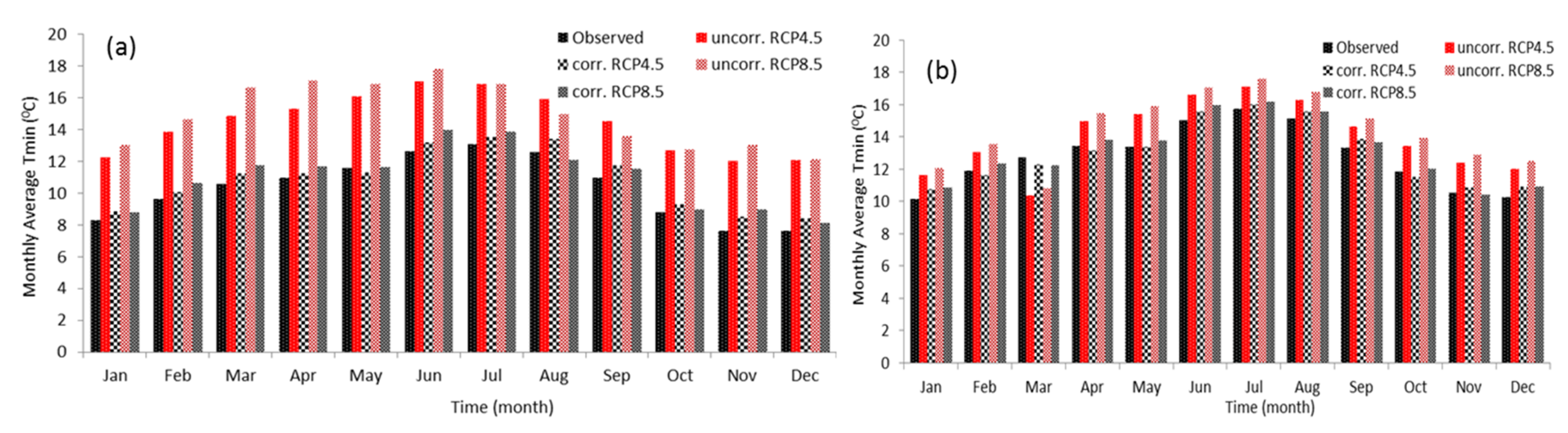
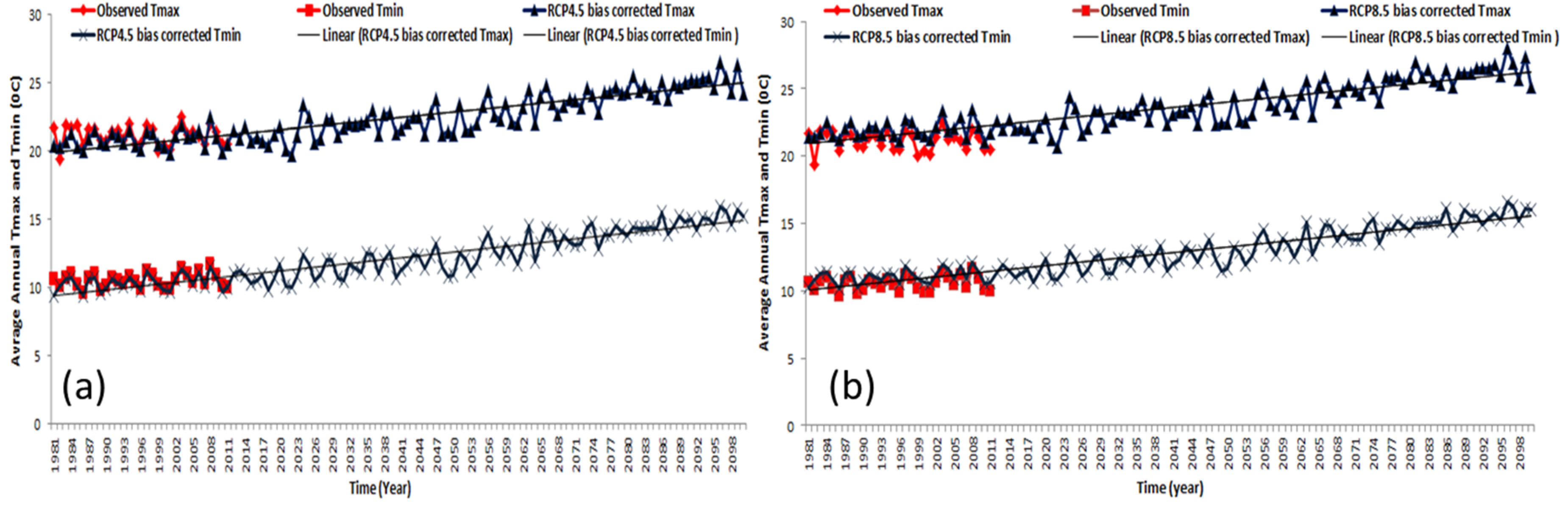
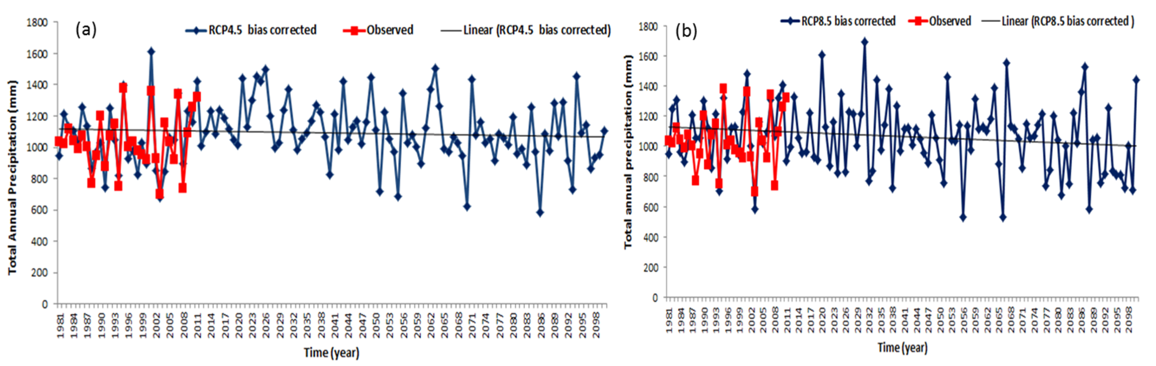
3.1. Precipitation and Temperature Bias Correction

The comparison of observed, uncorrected, and bias-corrected mean monthly rainfall data (1981–2010) is shown in Figure 2a,b. There was a considerable discrepancy between the uncorrected GCMs and observed data. The result revealed that both RCP4.5 and RCP8.5 overestimated the observed mean monthly precipitation for Addis Ababa station in January, February, March, June, July, November, and December; and underestimated for the remaining months. Concerning the Debrazeit station, the RCPs data overestimated the observed mean monthly precipitation for all months. Similarly, at each selected station located in the study area, the considered model with respective RCPs overestimated or underestimated the observed mean monthly rainfall for the baseline period (1981–2010). The result has shown that after monthly bias correction, the RCPs and observed rainfall exhibited similar patterns both at all stations. It was found that RCPs rainfall was reduced bias reasonably well after bias-corrected.

It can be seen that the two ensembles of bias-corrected GCMs seasonality fit well to the observed behavior: kiremt (JJAS) is the wet season (with rainfall peak in June), and the dry season occurs in Bega (ONDJ) and Belg (FMAM) (with the lowest amount of rainfall in December and January).

The uncorrected RCPs of maximum temperatures were overestimated for all stations and followed the pattern of the observed maximum temperature at Addis Ababa station. As shown in Figure 3a,b and Figure 4a,b, the uncorrected RCPs maximum and minimum temperature at each station were overestimated by the observed data almost for all months except for a few months. At Addis Ababa station, large differences between the observed and the uncorrected RCPs can be seen during the wet season. This shows that bias correction seems to correct bias reasonably well.

The correction coefficient of “a” and “b” obtained from the base periods was applied for the RCP4.5 and RCP8.5 to downscale the future rainfall and temperature scenarios. After the bias corrections were applied for the future RCPs, the estimated rainfall, maximum and minimum temperature had a similar pattern with the observed historical climate data. The bias-corrected RCP4.5 and RCP8.5 can be used for future hydrological impact assessments.

Downscaled future scenarios for the three climate variables (rainfall, maximum temperature, and minimum temperature) were graphically plotted to detect the trends. Results showed an increasing trend of average minimum and maximum temperature were observed for both RCP4.5 and RCP8.5 under all the time slices (Figure 5a,b), and decreasing trends were observed in total annual rainfall (Figure 6a,b), respectively.

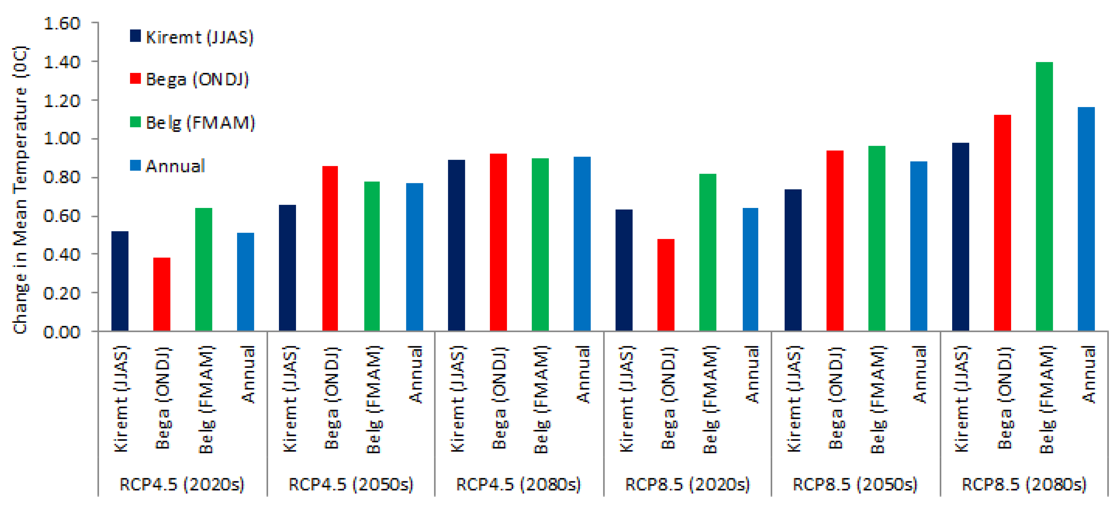
3.2. Change in Seasonal and Annual Temperature

The current research data revealed that the downscaled rainfall, maximum, and minimum temperatures increased in both emission scenarios. Annual and seasonal mean temperatures of the future periods (the 2020s, 2050s, and 2080s) for two ensemble GCMs models with RCP4.5 and RCP8.5 emissions scenarios are given in Figure 7. The projected ensemble data series showed an average annual and seasonal temperature increase. For the subbasin, the average annual temperature under RCP4.5 and RCP8.5 increases by 0.51 °C and 0.64 °C, respectively, in the 2020s. In mid-century, the annual temperature increases by 0.77 °C under RCP4.5 and 0.88 °C under RCP8.5; and increases by 0.9 °C under RCP4.5 and 1.2 °C under RCP8.5 by the end of the century. In the Awash River basin, the study also found that in mid-century minimum and maximum temperature increases range from 1.8 to 1.6 °C (RCP 4.5) to 2.6 to 2.1 °C (RCP8.5), respectively, while end-of-century increases vary from 2.4 to 2.0 °C (RCP 4.5) and 4.6 to 3.7 °C [79]. This shows the previous report overestimated temperature compared to the present results. Similarly, the finding Jilo et al. [80] argued that the mean annual maximum and minimum temperatures would increase under RCP4.5 and under RCP4.5 scenarios. Girma [81] has also argued that the increases of average annual temperature for the Upper Blue Nile Basin have been 1.5 °C for the 2020s, 2.6 °C for 2050s, and 4.5 °C for 2080s in relation to 1980–2010.

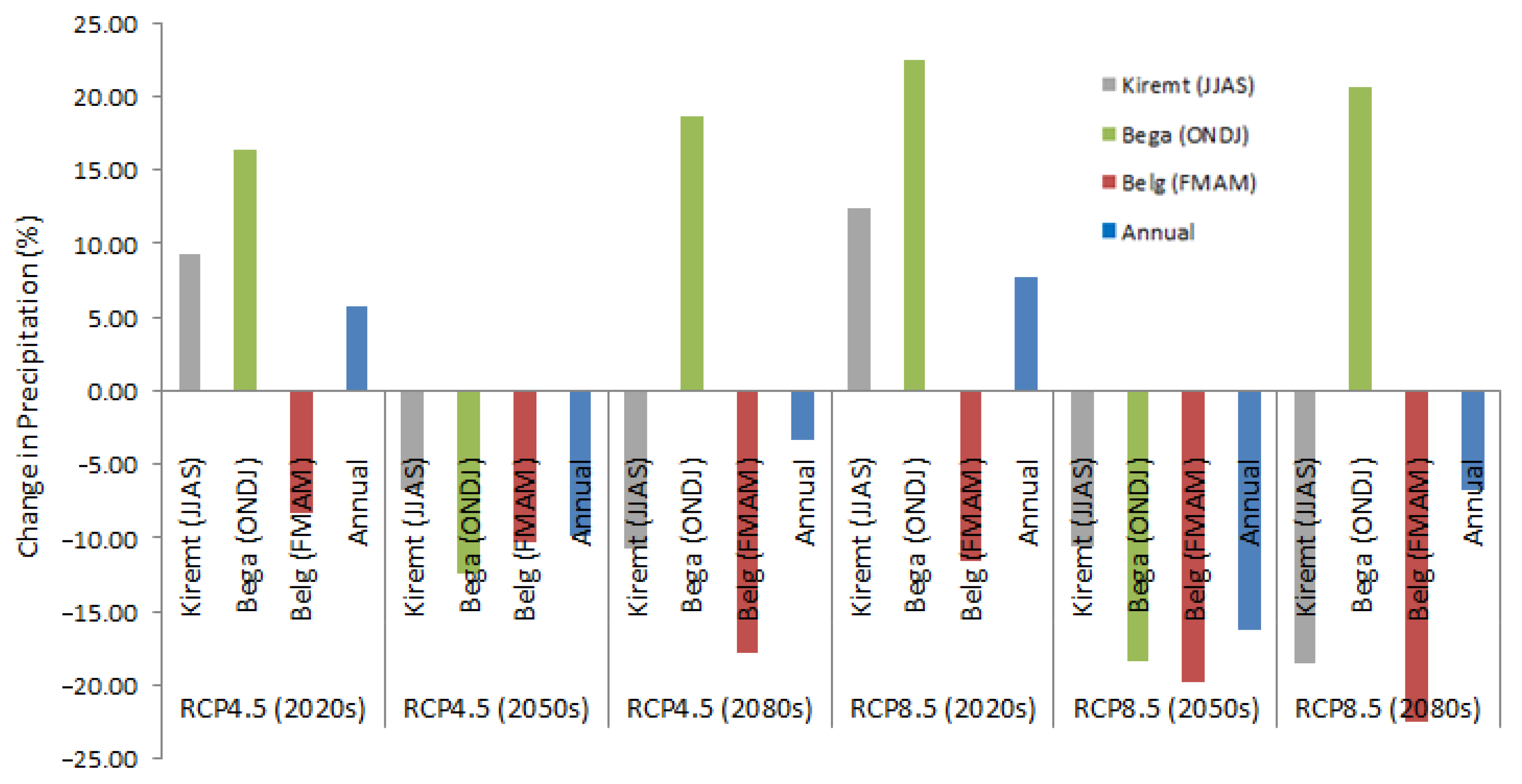
3.3. Change in Seasonal and Annual Rainfall

This study analyzed the projected annual and seasonal rainfall changes under RCP4.5 and RCP8.5 scenarios. Figure 8 shows the mean annual and seasonal rainfall changes for two ensembles GCMs. In the 2020s, the kiremt (JJAS) rainfall increases by 9.22% and 12.42% under RCP4.5 and RCP8.5, respectively, whereas it decreases by 6.82% for RCP4.5 and 10.74% for RCP8.5 in the 2050s; and 10.56% for RCP4.5 and 18.52% for RCP8.5 in the 2080s. The projected mean annual rainfall increases by 5.77% and 7.80% under RCP4.5 and RCP8.5 in the 2020s, respectively. On the contrary, for time periods 2050s and 2080s, projected annual rainfall decreases range 3.31 to 9.87% under RCP4.5 and 6.80 to 16.22% under RCP8.5. The maximum increments in mean seasonal rainfall can be seen in Bega (ONDJ) and Belg (FMAM) seasons under the RCP8.5 scenario in the 2080s, whereas minimum change can be seen in Bega (ONDJ) season in the 2020s under RCP4.5. Taye et al. [27] have also found the change in climate as projected by the GCMs shows a clear difference between seasons.

Generally, the results of simulated ensemble model scenarios to show drier conditions can be seen in the second rather than in the first half of the 21st-century. Girma [81] has found the ECHAM5 downscaled rainfall changed in the Upper Blue Nile by 1.8%, −6.6%, and −6.4% in the 2020s, 2050s, and 2080s, respectively. The result of this analysis coincides with the IPCC’s mid-range climate emission scenario, shows that, compared to the time period 1961–1990, annual precipitation undergoes changes from 0.6% to 4.9% and from 1.1% to 18.2% for 2030 and 2050, respectively [82].

As shown in previous results, climate models give estimated interpretations of real climate. Subsequently, applications of climate models are results to impact studies require consideration of several limitations that characterize model output. In principle, using the direct output of climate models is not desirable because these because of the limitations of coarse spatial resolution in the global models. Thus, downscaling will improve the performance of models and their ability to represent a physically consistent picture of the current and future climate conditions.

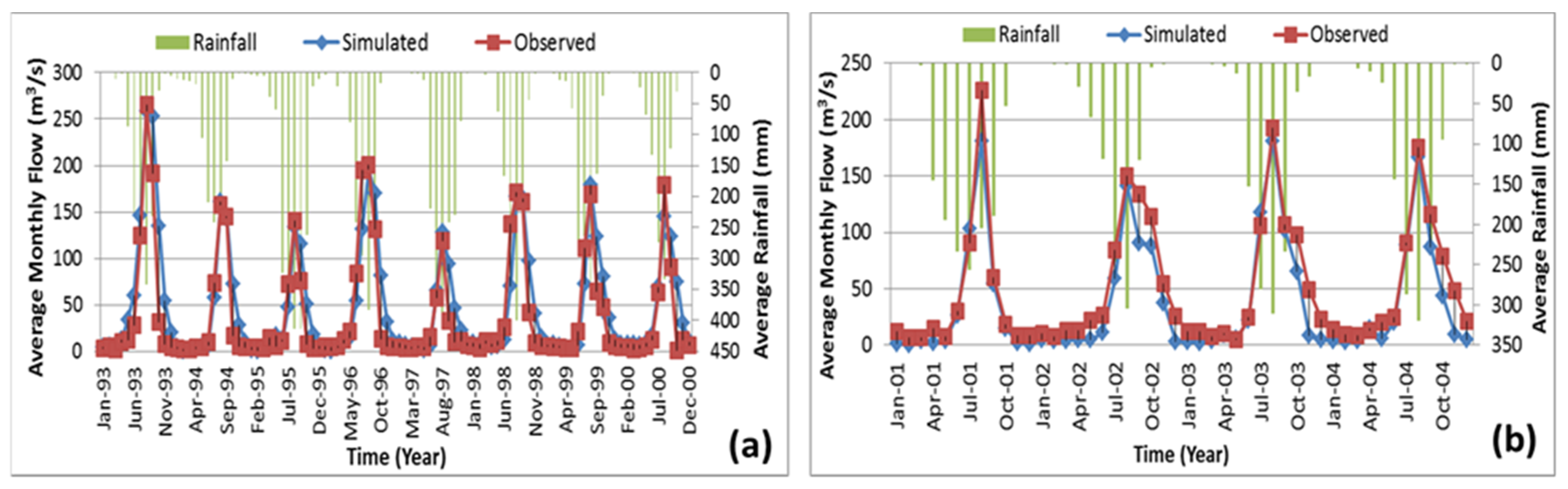
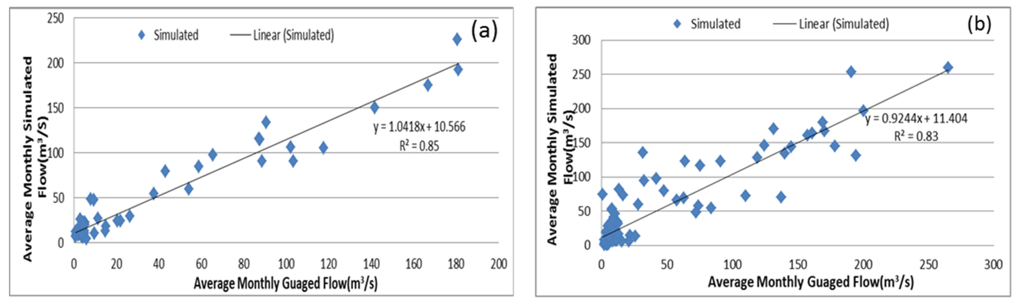
3.4. Flow Calibration and Validation

Calibration was performed for eight years period from 1 January 1993, to 31 December 2000, from which one year was taken as a warm-up period. As depicted in Figure 9, the calibration results showed that there is a good agreement between the simulated and gauged monthly flows at the outlet of the Hombole gauging station. Model statistical and performance indicators for streamflow simulations in the calibration and validation are shown in

Table 3. Model statistical and performance indicators for streamflow simulations in the calibration and validation periods.

Model	Calibration (1993–2000)	Validation (2001–2004)
ENS	0.80	0.78
R2	0.85	0.83
KGE	0.77	0.75
MAE	16.46	13.48
MBE	8.39	−12.35
RMSE	26.78	18.01

. This was demonstrated by the correlation coefficient (R² = 0.85), the Nash–Sutcliffe simulation efficiency (E_NS = 0.80), Kling-Gupta efficiency (KGE = 0.77), mean bias error (MBE = 8.39), mean absolute error (MAE = 16.46), and root mean square error (RMSE = 26.78). Similarly, the finding Shawul et al. [83] has found that the correlation coefficient (R² = 0.88) and the Nash–Sutcliffe simulation efficiency (E_NS = 0.87) showed a very good agreement between observed and simulated for the calibration period.

Validation proved the performance of the model for simulated flows in periods different from the calibration periods but without any further adjustment in the calibrated flows. Validation was performed for four years period from 1 January 2001, to 31 December 2004, from which one year was considered as a warm-up period. The correlation coefficient (R² = 0.83), the Nash–Sutcliffe simulation efficiency (E_NS = 0.78), Kling-Gupta efficiency (KGE = 0.75), mean bias error (MBE = −12.35), mean absolute error (MAE = 13.48), and root mean square error (RMSE = 18.01) showed a very good agreement between observed and simulated values. Both calibration and validation results fulfilled the requirements suggested by Santhi et al. [84] for R² > 0.6 and E_NS > 0.5 (Figure 9 and Figure 10). Shawul et al. [83] have argued that very good model performance was obtained at Hombole sub-basin with (R² = 0.88) and (E_NS = 0.87). Moreover, several studies have been reported that good to very good model performance was obtained in the study area [85,86,87], with E_NS and R² > 0.69, for the calibration and validation period. Thus, numerous studies have proven that the achieved model performance is satisfying.

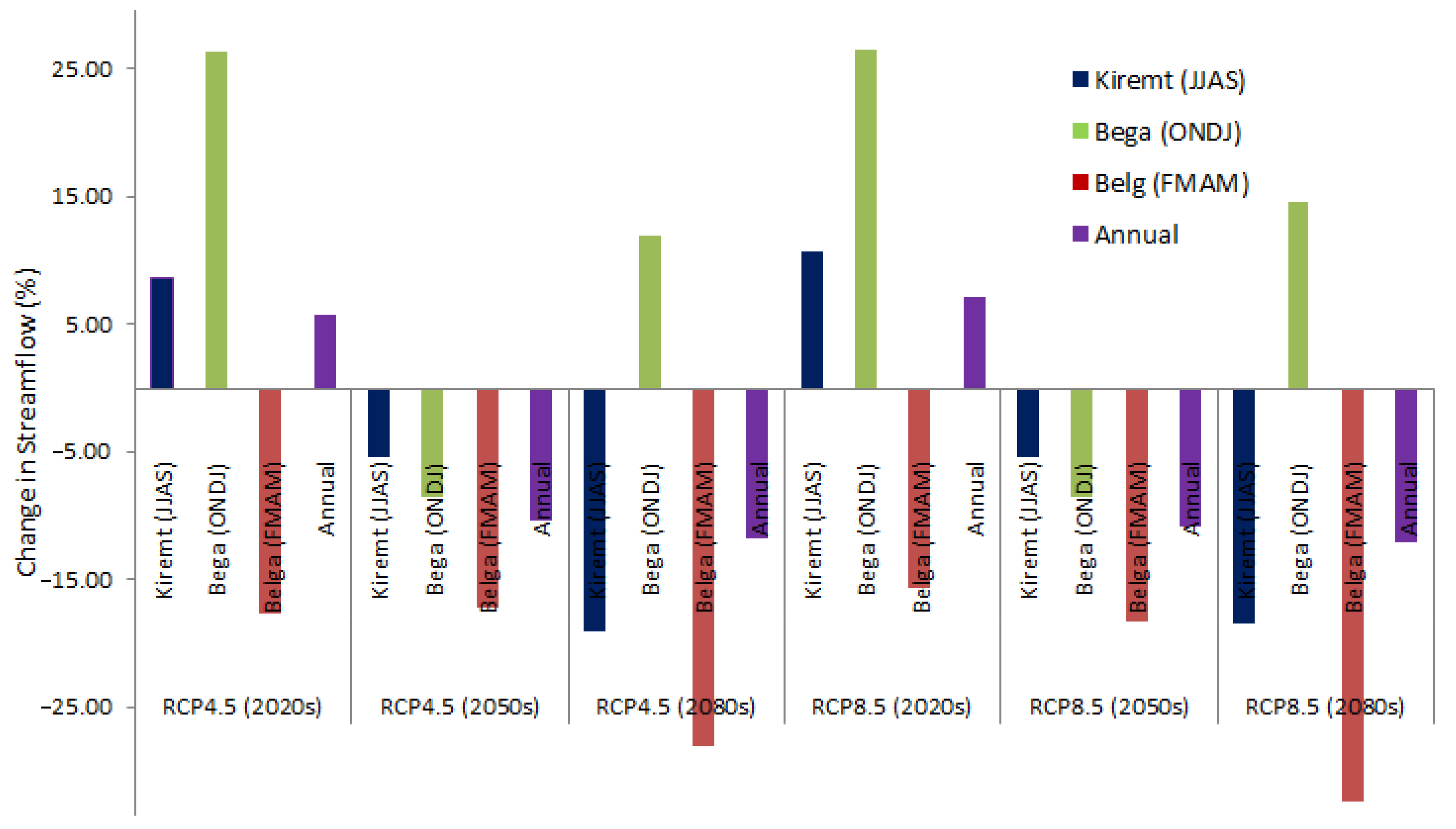
3.5. Climate Change Impact on Stream Flow

Climate change impact on monthly streamflow was analyzed by comparing baseline river flow with the future flows for three time periods (the 2020s, 2050s, and 2080s). Figure 11 showed the changes in average annual and seasonal streamflow (%) for the ensemble of two climate models for three-time slices under RCP4.5 and RCP8.5 emission scenarios. Results showed that Kiremt (JJAS) season streamflow increases by 8.61% for RCP4.5 and 10.66% for RCP8.5 in the 2020s, whereas decreases by 5.43% and 18.12% for RCP4.5 and 5.48% in the 2050s; and 19.42% for RCP8.5 in the 2080s. Similarly, annual streamflow increases by 5.80% under RCP4.5 and 7.20% under RCP8.5 for the period of the 2020s. The projected annual streamflow increases in the near-term and decreases in the middle and end of the 21st-century over the study area, ranging from −12.38 to 5.80%. The finding Getahun et al. [88] revealed the projected streamflow increase by 12% for the intermediate period in the subbasin.

The maximum reduction in streamflow can be seen in Belg (FMAM) season under both RCPs scenarios. Due to changes in precipitation and temperature, the annual and seasonal flow has changed, and the change is more serious during Kiremt and Belg (FMAM) seasons for period 2080s under RCP4.4 and RCP8.5. The maximum increase in streamflow can be seen in Bega (ONDJ) season by 26.56% in the 2020s under the RCP8.5 scenario.

The results suggested that the linkage between streamflow and precipitation may change in a future climate in that a unit decrease in precipitation will cause a larger decrease in streamflow for the middle and end centuries. This may be due to decreased recycling of moisture, more uniformly from year-to-year in a future wetter climate. The decrease in streamflow may associate with high temperatures and increased evapotranspiration [88]. Precipitation and temperature, being the main drivers in the water balance computation, in reference to their variability both annually and seasonally, have a direct impact on the other simulated water budget components. In agreement with the current finding, several reports on streamflow and runoff projections based on the SRES and RCP climate scenarios demonstrate a decrease in streamflow, surface runoff and water resources availability as a consequence of decreasing precipitation and increasing temperature [27,79,89,90,91,92,93]. Mersha et al. [42] have also found that under irrigation expansion scenario, streamflow will be reduced up to 23% during the last year of scenarios compared to the business-as-usual scenario, and this reduction streamflow likely imposes high pressure on water resources of the Upper Awash River basin.

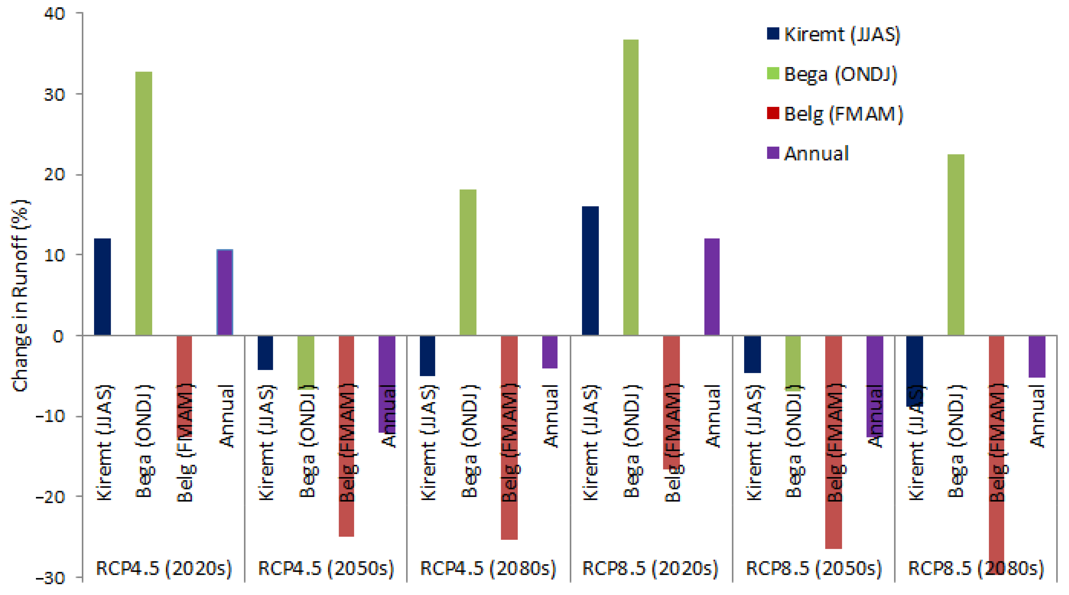
3.6. Climate Change Impact on Future Surface Runoff

Considering the daily observed meteorological and downscaled future RCPs data of rainfall and temperature as an input to the SWAT hydrological model, developed runoff projections were obtained for three future periods (the 2020s, 2050s, and 2080s). As shown in Figure 12, the annual surface runoff increments can be seen in the 2020s by 10.73% for RCP4.5 and 12.08% for RCP8.5, whereas decreases by 12.03% in the 2050s and 4.12% in the 2080s under RCP4.5; and 12.65% in the 2050s and 5.31% in the 2080s under RCP8.5. Similarly, the simulated flow in the 2020s showed increments of Bega (ONDJ) season runoff by 32.74% for RCP4.5 and 36.81% for RCP8.5 and in the 2080s, increases of 18.19% for RCP4.5 and 22.53% for RCP8.5 whereas decreases of 6.80% under RCP4.5 and 6.86% under RCP8.5 by the 2050s.

The projected average seasonal and annual runoff evaluation showed that runoff increases or decreases in magnitude in the future three periods as compared to the baseline period (1981–2010). A high amount of increase in average runoff was observed during Bega (ONDJ) season, whereas maximum reduction in runoff can be seen in the Belg (FMAM) season. Our study highlighted the change in projected streamflow and runoff across the upper Awash Subbasin because of decreased annual rainfall and increased temperature in the subbasin. Similar to the current result, climate change would have a significant impact on streamflow and surface runoff and water resources [27,79,88,94]. Daba [24] argued that climate variables (mainly rainfall and temperature) would have a significant effect on the surface runoff and causing a possible reduction in water availability. Abraham et al. [94] also found that a decrease in annual runoff and has been declining, particularly over the Meki and Katar River under RCP4.5 and RCP8.5 emission scenarios.

The projected runoff change is associated with the magnitude of rainfall and temperature changes over the basin in future periods. In agreement with the current finding, Taye et al. [27] concluded that in the Awash River basin, due to a projected increase in temperature and decrease in precipitation, the projections for the future three periods show an increase in water deficiency in all seasons. It was found that the projected increase/decrease of runoff associated with the increase/decrease in rainfall and temperature over the basin in the future time periods. The water resources sector will be impacted by climate change through a decrease in river runoff, as well as floods and droughts are on the increase [95]. The decrease in water availability throughout the future projected period’s indicator of water stress in the basin [27]. The inconsistency in the rainfall, which originates from climate change and variability, consequences in shortage of water stress; as a result, the ecosystem characterized among others by rain and water resource, could be seriously affected [7,8,11,80,96,97].

4. Conclusions

This specific study estimate the impacts of climate change on basin future runoff and streamflow supported the statistical downscaling technique. The ensemble of GCMs derived from the CSIRO-Mk3-6-0 and MIROC-ESM-CHEM with RCP4.5 and RCP8.5 was used for 3 future periods (the 2020s, 2050s, and 2080s) compared to the baseline period (1981–2010). The downscaling of climate variables like rainfall and temperature is very important for various impact studies in the Upper Awash River basin, which has huge water scarcity due to higher water demand, urbanization, economic development, and climatic variability in the basin. A statistical downscaling approach was employed to downscale these outputs at a station scale using the bias-correction method. The bias correction approach used in this study gave reasonable results. It was found that rainfall and temperature variances have been reduced significantly after bias correction. The performance statistics, including E_NS, R², KGE, MAE, MBE, and RMSE computed to evaluate the model performance, were more promising to simulate the future hydrology under a change in the climate.

The results showed that the projected average annual temperatures increase for all three time periods, whereas the predicted annual rainfall reduces for the period of the 2050s and 2080s and increases for period 2020s under both RCP4.5 and RCP8.5 scenarios. In the 2020s, the results of downscaled rainfall, maximum and minimum temperature increased in both RCP4.5 and RCP8.5 scenarios. These climate variable increments were expected to result in increases in the mean annual streamflow and runoff.

In this study, SWAT hydrological model was effectively applied to the annual and seasonal timescale to quantify climate change impacts on river flow for the subbasin. The results of hydrological model calibration and validation indicated that the SWAT model simulates appreciably well the streamflow for the area. The results of hydrological impacts of future climate change showed that there would be variation in components of mean annual and seasonal streamflow and runoff from current to future under both RCP4.5 and RCP8.5 scenarios. The seasonal effect would be more serious than the annual, due to the dominant dry seasons in the study area. Dry season change results would be more serious than that of the wet season in the basin. Climate change could cause an increased runoff in the wet season and a decreased runoff in the dry season, resulting in an increased seasonal variation in runoff and streamflow. The study revealed that climate change would have a significant impact on the surface runoff, on streamflow, and causing inconsistent increasing or decreasing water availability was observed. Thus, such studies would provide useful information for hydro-climatologists and managers for better decision-making regarding future agricultural and water resources management in the face of climate change.

5. Limitations and Recommendations

Even though this study employed a standard approach to evaluate the impacts of climate change on surface runoff and streamflow in the Upper Awash River Basin using an ensemble of two GCMs, a bias-correction scheme and a semi-distributed SWAT hydrological model, assessments can be improved by considering multiple GCMs, assess the impacts of possible soil and land-use changes, and uncertainties associated with future climate scenarios, bias-correction methods, and hydrological models. For instance, in the hydrological impact assessment, there are numerous sources of uncertainty. The climate models used, the SWAT model, and the bias correction of the GCMs outputs, have their levels of uncertainty. Even the use of an ensemble of the two GCMs for statistical downscaling may lead to biases in the estimation of future climate and hydrology. Thus, to take care of uncertainties using two GCMs, it is suggested to use a multimodel ensemble and/or multi scenarios approach to give a more accurate estimation of future hydrology. However, downscaling of the large-scale variables by using the bias correction method was done at some meteorological stations, and it was assumed that this alteration would be valid to other stations as well. However, it is recommendable if climate change assessment will be done by downscaling large-scale variables at each station located in the study area. Therefore, to reduce this uncertainty, further study using different GCMs outputs and use all RCPs emission scenarios and different downscaling methods need to be considered.

The same land use/cover data, as the current time, were used, and there is no consideration of changes in land-use, soil properties, which could influence the hydrology of the basin. Using more detailed hydrological models that combine the effects of land-use changes on the hydrological cycle and water obstructions on downstream flow may sharpen our insight and knowledge of future runoff and streamflow. Such a study should not be deliberated as an actual accurate scenario because the latter would need to include future land-use change impact. In addition to fluctuations in temperature and rainfall, non-climatic factors such as population growth, changes in water demand per capita and for agricultural needs, deforestation among current trends over the subbasin and can play a relevant role in the water resources of the Upper Awash subbasin. Thus, the study strongly recommends a thorough study of the combined effect of non-climatic factors, climate and land use/land cover change on the water recourses variability and hydrological processes, which are so crucial for the livelihoods and economy of people.

Despite these limitations, this study is a good starting point to assess future flows, and further research is recommended to address the limitations of this study for improved understanding and assessments that will prove useful for better planning and management of water resources in the basin.

References

1. IPCC. Summary for Policymakers. In Climate Change 2014: The Physical Science Basis; Contribution of Working Group I to the IPCC Fifth Assessment Report Climate Change; Cambridge University Press: Cambridge, UK; New York, NY, USA, 2014. [Google Scholar]
2. Boru, G.F.; Gonfa, Z.B.; Diga, G.M. Impacts of climate change on stream flow and water availability in Anger sub-basin, Nile Basin of Ethiopia. Sustainable. Water Resour. Manag. 2019, 5, 1755–1764. [Google Scholar] [CrossRef]
3. IPCC. Climate Change 2013: The Physical Science Basis Contribution of Working Group I to the Fifth Assessment Report of the Intergovernmental Panel on Climate Change; Stocker, T.F., Qin, D., Plattner, G.K., Tignor, M.M., Allen, S.K., Boschung, J., Nauels, A., Xia, Y., Bex, V., Midgley, P.M., Eds.; Cambridge University Press: Cambridge, UK; New York, NY, USA, 2013; p. 1535. [Google Scholar]
4. Mahmood, R.; Babel, M.S. Evaluation of SDSM developed by annual and monthly sub-models for downscaling temperature and precipitation in the Jhelum basin, Pakistan and India. Theor. Appl. Climatol. 2013, 113, 27–44. [Google Scholar] [CrossRef]
5. Vose, J.M.; Clark, J.S.; Luce, C.H. Introduction to drought and US forests: Impacts and potential management responses. Ecol. Manag. 2016, 380, 296–298. [Google Scholar] [CrossRef]
6. Kerns, B.K.; Powell, D.C.; Mellmann-Brown, S.; Carnwath, G.; Kim, J.B. Effects of projected climate change on vegetation in the Blue Mountains Eco-region, USA. Clim. Serv. 2018, 10, 33–43. [Google Scholar] [CrossRef]
7. Hartter, J.; Hamilton, L.C.; Boag, A.E.; Stevens, F.R.; Ducey, M.J.; Christoffersen, N.D.; Oester, P.T.; Palace, M.W. Does it matter if people think climate change is human caused? Clim. Serv. 2018, 10, 53–62. [Google Scholar] [CrossRef]
8. Caty, F.C.; Kate, T.D.; Charles, H.L.; Gordon, E.G.; Mohammad, S.; Jessica, E.H.; Brian, P.S. Effects of climate change on hydrology and water resources in the Blue Mountains, Oregon, USA. Clim. Serv. 2018, 10, 9–19. [Google Scholar]
9. Farsani, F.I.; Farzaneh, M.R.; Besalatpour, A.A.; Salehi, M.H.; Faramarzi, M. Assessment of the impact of climate change on spatiotemporal variability of blue and green water resources under CMIP3 and CMIP5 models in a highly mountainous watershed. Theor. Appl. Climatol. 2019, 136, 169–184. [Google Scholar] [CrossRef]
10. UNWWAP. The United Nations World Water Development Report 2018: Nature-Based Solutions for Water; UNESCO: Paris, France, 2018. [Google Scholar]
11. Peterson, D.L.; Halofsky, J.E. Adapting to the effects of climate change on natural resources in the Blue Mountains, USA. Clim. Serv. 2018, 10, 63–71. [Google Scholar] [CrossRef]
12. IPCC. Impacts, Adaptation and Vulnerability. Part A: Global and Sectoral Aspects. In Contribution of Working Group II to the Fifth Assessment Report of the Intergovernmental Panel on Climate Change; Field, C.B., Barros, V.R., Dokken, D.J., Mach, K.J., Mastrandrea, M.D., Bilir, T.E., Chatterjee, M., Ebi, K.L., Estrada, Y.O., Genova, R.C., et al., Eds.; Cambridge University Press: Cambridge, UK; New York, NY, USA, 2014. [Google Scholar]
13. Zhang, W.; Zha, X.; Li, J.; Liang, W.; Ma, Y.; Fan, D.; Li, S. Spatiotemporal change of blue water and green water resources in the Headwater of Yellow River Basin, China. Water Resour. Manag. 2014, 28, 4715–4732. [Google Scholar] [CrossRef]
14. Reshmidevi, T.V.; Nagesh Kumar, D.; Mehrotra, R.; Sharma, A. Estimation of the climate change impact on a catchment water balance using an ensemble of GCMs. J. Hydrol. 2018, 556, 1192–1204. [Google Scholar] [CrossRef] [Green Version]
15. Jin, X.; Sridhar, V. Impacts of Climate Change on Hydrology and Water Resources in the Boise and Spokane River Basins. J. Am. Water Resour. Assoc. 2011, 48, 197–220. [Google Scholar] [CrossRef]
16. Kundzewicz, Z.W. Climate change impacts on the hydrological cycle. Ecohydrol. Hydrobio. 2008, 8, 195–203. [Google Scholar] [CrossRef] [Green Version]
17. Silva, V.; Silva, M.T.; Singh, V.P.; Souza, E.P.; Braga, C.C.; Holanda, R.M.; Almeida, R.S.; Sousa, A.S.F.; Braga, A.C.R. Simulation of stream flow and hydrological response to land-cover changes in a tropical river basin. Catena 2018, 16216, 61–76. [Google Scholar]
18. Mango, L.; Melesse, A.M.; McClain, M.E.; Gann, D.; Setegn, S.G. Land use and climate change impacts on the hydrology of the upper Mara River Basin, Kenya: Results of a modeling study to support better resource management. Hydrol. Earth. Syst. Sci. 2011, 15, 224–2258. [Google Scholar] [CrossRef] [Green Version]
19. Mango, L.; Melesse, A.M.; McClain, M.E.; Gann, D.; Setegn, S.G. Hydro-Meteorology and Water Budget of Mara River Basin, Kenya: A Land Use Change Scenarios Analysis (Chap. 2); Nile River Basin: Hydrology, Climate and Water Use; Melesse, A.M., Ed.; Springer Science Publisher: Berlin/Heidelberg, Germany, 2011; pp. 39–68. [Google Scholar] [CrossRef]
20. Behulu, F.; Setegn, S.; Melesse, A.M.; Romano, E.; Fiori, A. Impact of climate change on the hydrology of Upper Tiber River Basin Using bias corrected regional climate model. Water Resour. Manag. 2014, 28, 1327–1343. [Google Scholar]
21. Setegn, S.G.; David, R.; Melesse, A.M.; Bijan, D.; Ragahavan, S.; Anders, W. Climate Change Impact on Agricultural Water Resources Variability in the Northern Highlands of Ethiopia. In Nile River Basin; Springer: Dordrecht, The Netherlands, 2011; pp. 241–265. [Google Scholar]
22. Setegn, S.; Melesse, A.M. Climate Change Impact on Water Resources and Adaptation Strategies in the Blue Nile River Basin. In Nile River Basin: Ecohydrological Challenges, Climate Change and Hydropolitics; Melesse, A.M., Abtew, W., Setegn, S., Eds.; Springer: Cham, Switzerland, 2014; pp. 389–404. [Google Scholar]
23. Assefa, T.; Anwar, A.; Melesse, A.M.; Admasu, S. Climate Change in Upper Gilgel Abay River Catchment, Blue Nile Basin Ethiopia. In Nile River Basin: Ecohydrological Challenges, Climate Change and Hydropolitics; Melesse, A.M., Abtew, W., Setegn, S., Eds.; Springer Science & Business Media: Berlin/Heidelberg, Germany, 2014; pp. 363–388. [Google Scholar]
24. Daba, M.H. Sensitivity of SWAT Simulated Runoff to Temperature and Rainfall in the Upper Awash Sab-Basin, Ethiopia. Hydrol. Curr. Res. 2018, 9, 293. [Google Scholar] [CrossRef]
25. Daba, M.; Rao, G.N. Evaluating Potential Impacts of Climate Change on Hydro- meteorological Variables in Upper Blue Nile Basin, Ethiopia: A Case Study of Finchaa Sub-basin. J. Environ. Earth Sci. 2016, 6, 48–57. [Google Scholar]
26. Chang, H.; Jung, I.W. Spatial and temporal changes in runoff caused by climate change in a complex large river basin in Oregon. J. Hydrol. 2010, 388, 186–207. [Google Scholar] [CrossRef]
27. Taye, M.; Dyer, E.; Hirpa, F.; Charles, K. Climate change impact on water resources in the Awash basin, Ethiopia. Water 2018, 10, 1560. [Google Scholar] [CrossRef] [Green Version]
28. Gan, T.Y. Reducing vulnerability of water resources of Canadian prairies to potential droughts and possible climatic warming. Water Resour. Manag. 2000, 14, 111–135. [Google Scholar] [CrossRef]
29. Xu, C.Y. Modeling the effects of climate change on water resources in central Sweden. Water Resour. Manag. 2000, 14, 177–189. [Google Scholar] [CrossRef]
30. Arora, M.; Singh, P.; Goel, N.K.; Singh, R.D. Climate variability influences on hydrological responses of a large Himalayan basin. Water Resour. Manag. 2008, 22, 1461–1475. [Google Scholar] [CrossRef]
31. Givati, A.; Thirel, G.; Rosenfeld, D.; Paz, D. Climate change impacts on streamflow at the upper Jordan River based on an ensemble of regional climate models. J. Hydrol. Reg. Stud. 2019, 21, 92–109. [Google Scholar] [CrossRef]
32. Hailemariam, K. Impact of climate change on the water resources of Awash River Basin, Ethiopia. Clim. Res. 1999, 12, 91–96. [Google Scholar] [CrossRef] [Green Version]
33. Behailu, S. Stream Flow Simulation for the Upper Awash Basin. Master’s Thesis, Department of Civil Engineering, Addis Ababa University, Addis Ababa, Ethiopia, 2004; pp. 63–75. [Google Scholar]
34. Mengistu, D.T. Regional Flood Frequency Analysis for Upper Awash Sub-basin (Upstream of Koka). Master’s Thesis, Addis Ababa University, Addis Ababa, Ethiopia, 2008; pp. 66–87. [Google Scholar]
35. Surur, A.N. Simulated Impact of Land Use Dynamics on Hydrology during a 20-year-period of Beles Basin in Ethiopia. Master’s Thesis, Water System Technology Department of Land and Water Resources Engineering, Stockholm, Sweden, 2010. [Google Scholar]
36. Kurkura, M.; Michael, Y. Water Balance of Upper awash Basin Based on Satellite-Derived Data (Remote Sensing). Master’s Thesis, Addis Ababa University, Addis Ababa, Ethiopia, 2011. [Google Scholar]
37. Taddese, G.; Sonder, K.; Peden, D. The Water of the Awash River Basin a Future Challenge to Ethiopia; ILRI: Addis Ababa, Ethiopia, 2012; p. 13. [Google Scholar]
38. Bang, H.Q.; Quan, N.H.; Phu, V.L. Impacts of Climate Change on Catchment Flows and Assessing Its Impacts on Hydropower in Vietnam’s Central Highland Region. Glob. Perspect. Geogr. 2013, 1, 1. [Google Scholar]
39. Mengistu, D.T.; Sorteberg, A. Sensitivity of SWAT simulated stream flow to climatic changes within the Eastern Nile River basin. Hydrol. Earth Syst. Sci. 2012, 16, 391–407. [Google Scholar] [CrossRef] [Green Version]
40. Demissie, T.A.; Saathoff, F.; Sileshi, Y.; Gebissa, A. Climate change impacts on the stream flow and simulated sediment flux to Gilgel Gibe 1 hydropower reservoir, Ethiopia. European. Int. J. Sci. Technol. 2013, 2, 2304–9693. [Google Scholar]
41. Chekol, D.A. Application of SWAT for assessment of spatial distribution of water resources and analyzing impact of different land management practices on soil erosion in Upper Awash River Basin watershed. FWU Water Resour. Publ. 2007, 6, 110–117. [Google Scholar]
42. Mersha, A.; Masih, I.; Fraiture, C.; Wenninger, J.; Alamirew, T. Evaluating the Impacts of IWRM Policy Actions on Demand Satisfaction and Downstream Water Availability in the Upper Awash Basin, Ethiopia. Water 2018, 10, 892. [Google Scholar] [CrossRef] [Green Version]
43. Lupo, A.; Kininmonth, W.; Armstrong, J.; Green, K. Global climate models and their limitations. Clim. Chang. Reconsidered II Phys. Sci. 2013, 9, 148. [Google Scholar]
44. Bader, D.C.; Covey, C.; Gutowski, W.; Held, I.; Kunkel, K.; Miller, R.; Tokmakian, R.; Zhang, M. Climate Models: An Assessment of Strengths and Limitations; U.S. Department of Energy: Washington, DC, USA, 2008.
45. Legates, D.R. Limitations of climate models as predictors of climate change. Brief Anal. 2002, 396, 1–2. [Google Scholar]
46. Schneider, S.H.; Dickinson, R.E. Climate modeling. Rev. Geophys. 1974, 12, 447–493. [Google Scholar] [CrossRef]
47. Bajracharya, A.R.; Sagar, R.B.; Arun, B.S.; Sudan, B.M. Climate change impact assessment on the hydrological regime of the Kaligandaki Basin, Nepal. Sci. Total Environ. 2018, 625, 837–848. [Google Scholar] [CrossRef] [PubMed]
48. Vaghefi, A.S.; Mousavi, S.J.; Abbaspour, K.C.; Srinivasan, R.; Yang, H. Analyses of the impact of climate change on water resources components, drought and wheat yield in semiarid regions: Karkheh River Basin in Iran. Hydrol. Process. 2014, 28, 2018–2032. [Google Scholar] [CrossRef]
49. Li, Z.; Lü, Z.; Li, J.; Shi, X. Links between the spatial structure of weather generator and hydrological modeling. Appl. Clim. 2015, 128, 103–111. [Google Scholar] [CrossRef]
50. Shrestha, S.; Shrestha, M.; Babel, M.S. Modelling the potential impacts of climate change on hydrology of Indrawati River Basin in Nepal. Environ. Earth Sci. 2015, 75, 280. [Google Scholar] [CrossRef]
51. Dessu, S.B.; Melesse, A.M. Impact and uncertainties of climate change on the hydrology of the Mara River Basin. Hydrol. Proc. 2013, 27, 2973–2986. [Google Scholar]
52. Dessu, S.B.; Melesse, A.M.; Bhat, M.; McClain, M. Assessment of water resources availability and demand in the Mara River Basin. Catena 2014, 115, 104–114. [Google Scholar] [CrossRef]
53. Behulu, F.; Setegn, S.; Melesse, A.M.; Fiori, A. Hydrological analysis of the Upper Tiber Basin: A watershed modeling approach. Hydrol. Proc. 2013, 27, 2339–2351. [Google Scholar]
54. Getachew, H.E.; Melesse, A.M. Impact of land use/land cover change on the hydrology of Angereb watershed, Ethiopia. Int. J. Water Sci. 2012, 1, 6. [Google Scholar]
55. Grey, O.P.; Webber, D.G.; Setegn, S.G.; Melesse, A.M. Application of the soil and water assessment tool (SWAT model) on a small tropical island state (Great River Watershed, Jamaica) as a tool in integrated watershed and coastal zone management. Int. J. Trop. Biol. Conserv. 2013, 62, 293–305. [Google Scholar]
56. Mohammed, H.; Alamirew, T.; Assen, M.; Melesse, A.M. Modeling of sediment yield in Maybar gauged watershed using SWAT, Northeast Ethiopia. Catena 2015, 127, 191–205. [Google Scholar]
57. OWWDSE. Upper Awash Integrated Land uses Planning Study Project. Unpublished Interim Rep. 2013. [Google Scholar]
58. Berhe, F.; Melesse, A.M.; Hailu, D.; Seleshi, Y. Water use allocation modeling using MODISM in the Awash River basin. Catena 2013, 109, 118–128. [Google Scholar] [CrossRef]
59. Yang, W.; Seager, R.; Cane, M.A.; Lyon, B. The East African long rains in observations and models. J. Clim. 2014, 27, 7185–7202. [Google Scholar] [CrossRef]
60. Sorecha, E.M.; Kibret, K.; Hadgu, G.; Lupi, A. Exploring the impacts of climate change on chickpea (Cicer arietinum L.) production in central highlands of Ethiopia. Acad. Res. J. Agric. Sci. Res. 2017, 5, 140–150. [Google Scholar]
61. Bathiany, S.; Dakos, V.; Scheffer, M.; Lenton, T.M. Climate models predict increasing temperature variability in poor countries. Sci. Adv. 2018, 4, eaar5809. [Google Scholar] [CrossRef] [Green Version]
62. Mumo, L.; Jinhua, Y. Gauging the performance of CMIP5 historical simulation in reproducing observed gauge rainfall over Kenya. Atmos. Res. 2019, 236, 104808. [Google Scholar] [CrossRef]
63. Zebaze, S.; Jain, S.; Salunke, P.; Shafiq, S.; Mishra, S.K. Assessment of CMIP5 multimodal mean for the historical climate of Africa. Atmos. Sci. Lett. 2019, 20, e926. [Google Scholar] [CrossRef] [Green Version]
64. Van Vuuren, D.P.; Den Elzen, M.G.; Lucas, P.L.; Eickhout, B.; Strengers, B.J.; Van Ruijven, B.; Van Houdt, R. Stabilizing greenhouse gas concentrations at low levels: An assessment of reduction strategies and costs. Clim. Chang. 2007, 81, 119–159. [Google Scholar] [CrossRef] [Green Version]
65. Rogelj, J.; Meinshausen, M.; Knutti, R. Global warming under old and new scenarios using IPCC climate sensitivity range estimates. Nat. Clim. Chang. 2012, 2, 248. [Google Scholar] [CrossRef]
66. Neitsch, S.I.; Arnold, J.G.; Kinrv, J.R.; Williams, J.R. Soil and Water Assessment Tool, Theoretical Documentation; USDA Agricultural Research Service Texas A and M Black land Research Center: Temple, TX, USA, 2005. [Google Scholar]
67. Arnold, J.G.; Srinivasan, R.; Muttiah, R.S.; Williams, J.R. Large-area hydrologic modeling and assessment: Part I Model development. JAWRA J. Am. Water Resour. Assoc. 1998, 34, 73–89. [Google Scholar] [CrossRef]
68. Neitsch, S.L.; Arnold, J.G.; Kiniry, J.R.; Williams, J.R.; King, K.W. Soil and Water Assessment Tool, Theoretical Documentation and User’s Manual; Texas Water Resources Institute: Forney, TX, USA, 2002. [Google Scholar]
69. Cunderlik, J. Hydrologic Model Selection for the CFCAS Project: Assessment of Water Resources Risk and Vulnerability to Changing Climatic Conditions; Project Report; Department of Civil and Environmental Engineering, University of Western Ontario: London, UK, 2003. [Google Scholar]
70. SCS (Soil Conservation Service). National Engineering Handbook; Section 4; U.S. Department of Agriculture: Washington, DC, USA, 1972.
71. Green, W.H.; Ampt, G.A. Studies on soil physics, the flow of air and water through soils. J. Agric. Sci. 1911, 4, 11–24. [Google Scholar]
72. Smitha, P.S.; Narasimhan, B.; Sudheer, K.P.; Annamalai, H. An improved bias correction method of daily rainfall data using a sliding window technique for climate change impact assessment. J. Hydrol. 2018, 556, 100–118. [Google Scholar] [CrossRef]
73. Teutschbein, C.; Seibert, J. Bias correction of regional climate model simulations for hydrological Climate-change impact studies: Review and evaluation of different methods. J. Hydrol. 2012, 456, 12–29. [Google Scholar] [CrossRef]
74. Leander, R.; Buishand, T.A. Resampling of regional climate model output for the simulation of Extreme River flows. J. Hydrol. 2007, 332, 487–496. [Google Scholar] [CrossRef]
75. Terink, W.; Hurkmans, R.; Torfs, P.; Uijlenhoet, R. Evaluation of a bias correction method applied to downscaled precipitation and temperature reanalysis data for Rhine Basins. J. Hydrol. Earth Syst. Sci. 2009, 6, 5377–5413. [Google Scholar] [CrossRef] [Green Version]
76. Ho, C.; Stephenson, D.; Collins, M.; Ferro, C.; Brown, S. Calibration strategies: A Source of Additional Uncertainty in Climate Change Projections. Bull. Am. Meteorol. Soc. 2012, 93, 21–26. [Google Scholar] [CrossRef] [Green Version]
77. Nash, J.E.; Sutcliffe, J.V. River flow forecasting through conceptual models. Part I: A discussion of principles. J. Hydrol. 1970, 10, 282–290. [Google Scholar] [CrossRef]
78. Bayazit, M. Nonstationarity of hydrological records and recent trends in trend analysis: A state-of-the-art review. Environ. Process. 2015, 2, 527–542. [Google Scholar] [CrossRef]
79. Bekele, D.; Alamirew, T.; Kebede, A.; Zeleke, G.; Melesse, A.M. Modeling climate change impact on the Hydrology of Keleta watershed in the Awash River basin, Ethiopia. Environ. Modeling Assess. 2019, 24, 95–107. [Google Scholar] [CrossRef]
80. Jilo, N.B.; Gebremariam, B.; Harka, A.E.; Woldemariam, G.W.; Behulu, F. Evaluation of the Impacts of Climate Change on Sediment Yield from the Logiya Watershed, Lower Awash Basin, Ethiopia. Hydrology 2019, 6, 81. [Google Scholar] [CrossRef] [Green Version]
81. Girma, M. Potential Impact of Climate and Land Use Changes on the Water Resources of the Upper Blue Nile Basin. Ph.D. Thesis, Department of Earth Sciences Institute for Geographical Sciences, Physical Geography Freie University of Berlin, Berlin, Germany, 2012. [Google Scholar]
82. NMA. National Meteorological Agency Seasonal Agro Meteorology Bulletin Report; NMA: Addis Ababa, Ethiopia, 2006. [Google Scholar]
83. Shawul, A.A.; Chakma, S.; Melesse, A.M. The response of water balance components to land covers change based on hydrologic modeling and partial least squares regression (PLSR) analysis in the Upper Awash Basin. J. Hydrol. Reg. Stud. 2019, 26, 100640. [Google Scholar] [CrossRef]
84. Santhi, C.; Arnold, J.G.; Williams, J.R.; Dugas, W.A.; Srinivasan, R.; Hauck, L.M. Validation of the SWAT model on a large river basin with point and nonpoint sources. J. Am. Water Resour. Assoc. 2001, 37, 1169–1188. [Google Scholar] [CrossRef]
85. Amin, A.; Nuru, N. Evaluation of the Performance of SWAT Model to Simulate Stream Flow of Mojo River Watershed: In the Upper Awash River Basin, in Ethiopia. Hydrology 2020, 8, 7. [Google Scholar] [CrossRef]
86. Biru, Z.; Kumar, D. Calibration and validation of SWAT model using stream flow and sediment load for Mojo watershed, Ethiopia. Sustain. Water Resour. Manag. 2018, 4, 937–949. [Google Scholar] [CrossRef]
87. Getu, M. Impact of Climate Change on Hydrological Response of Mojo River Catchment Awash River Basin. Master’s Thesis, Bahir Dar University, Bahir Dar, Ethiopia, 2020. [Google Scholar]
88. Getahun, Y.S.; van Lanen, I.H.; Torfs, P.P. Impact of Climate Change on Hydrology of the Upper Awash River Basin (Ethiopia): Inter-comparison of Old SRES and New RCP Scenarios. Ph.D. Thesis, Wageningen University, Wageningen, The Netherlands, 2014. [Google Scholar]
89. Lijalem, Z.A.; Jackson, R.; Chekol, D.A. Climate Change Impact on Lake Ziway Watershed Water Availability, Ethiopia. Unpublished Master’s Thesis, Institute for Technology in the Tropics, University of Applied Science, Cologne, Germany, 2007. [Google Scholar]
90. Yang, W. Trends and responses to global change of China’s arid regions. Front. For. China 2009, 4, 255–262. [Google Scholar] [CrossRef]
91. Ghosh, S.; Misra, C. Assessing Hydrological Impacts of Climate Change. Modeling Techniques and Challenges. Open Hydrol. J. 2010, 4, 115–121. [Google Scholar] [CrossRef]
92. Tatenda, L.; Gete, Z.; Caroline, A.; Luciano, G.; Hannes, S.; Vincent, R. Modelling the effect of soil and water conservation on discharge and sediment yield in the upper Blue Nile basin, Ethiopia. Appl. Geogr. 2016, 73, 89–101. [Google Scholar]
93. Solomon, M. Effect of Climate Change on Water Resources. J. Water Resour. Ocean Sci. 2016, 5, 14–21. [Google Scholar]
94. Abraham, T.; Abate, B.; Woldemicheal, A.; Muluneh, A. Impacts of Climate Change under CMIP5 RCP Scenarios on the Hydrology of Lake Ziway Catchment, Central Rift Valley of Ethiopia. J. Environ. Earth Sci. 2018, 8, 7. [Google Scholar]
95. Tadege, A. Climate Change National Adaptation Program of Action (NAPA) of Ethiopia; National Meteorological Agency (NMA): Addis Ababa, Ethiopia, 2007.
96. Zeray, N.; Demie, A. Climate Change Impact, Vulnerability and Adaptation Strategy in Ethiopia: A Review. J. Environ. Earth Sci. 2015, 5, 21. [Google Scholar]
97. Daba, M.H.; Ayele, G.T.; Songcai, Y. Long-term homogeneity and trends of hydroclimatic variables in upper Awash River basin, Ethiopia. Adv. Meteorol. 2020, 2020, 1–21. [Google Scholar] [CrossRef]
Figure 1. Study area location of the Upper Awash River Basin.
Hydrology 07 00098 g001
Figure 2. Bias corrected precipitation at (a) Addis Ababa and (b) Debrazeit stations.
Hydrology 07 00098 g002
Figure 3. Bias corrected maximum temperature at (a) Addis Ababa and at (b) Debrazeit stations.
Hydrology 07 00098 g003
Figure 4. Bias corrected minimum temperature at (a) Addis Ababa and at (b) Debrazeit stations.
Hydrology 07 00098 g004
Figure 5. Future trends of (a) representative concentration pathways (RCP4.5) and (b) representative concentration pathways (RCP8.5) maximum and minimum mean annual temperatures (1981–2100).
Hydrology 07 00098 g005
Figure 6. Future trends of (a) RCP4.5 and (b) RCP8.5 total mean annual rainfall (1981–2100).
Hydrology 07 00098 g006
Figure 7. Change in seasonal and annual temperature for three time periods under RCP4.5 and RCP8.5.
Hydrology 07 00098 g007
Figure 8. Seasonal and annual change in rainfall for three time periods under RCP4.5 and RCP8.5.
Hydrology 07 00098 g008
Figure 9. Hydrographs of monthly simulated and gauged flows for calibration (a) and validation (b) at the outlet of the Hombole station.
Hydrology 07 00098 g009
Figure 10. Scatter plot of monthly simulated and gauged flow for (a) calibration and (b) validation periods at Hombole station.
Hydrology 07 00098 g010
Figure 11. Seasonal and annual change in streamflow for three time periods under RCP4.5 and RCP8.5.
Hydrology 07 00098 g011
Figure 12. Seasonal and annual change in runoff for three time periods under RCP4.5 and RCP8.5.
Hydrology 07 00098 g012