Article

A One-Way Coupled Hydrodynamic Advection-Diffusion Model to Simulate Congested Large Wood Transport

by
Elisabetta Persi
1,*,
Gabriella Petaccia
1,
Stefano Sibilla
1,
Roberto Bentivoglio
2 and
Aronne Armanini
3
1
Department of Civil Engineering and Architecture, University of Pavia, via Ferrata, 3, 27100 Pavia, Italy
2
Department of Water Management, Delft University of Technology, Stevinweg, 1, 2628 CN Delft, The Netherlands
3
Department of Civil, Environmental and Mechanical Engineering, University of Trento, via Mesiano, 77, 38123 Trento, Italy
*
Author to whom correspondence should be addressed.
Submission received: 28 December 2020 / Revised: 21 January 2021 / Accepted: 24 January 2021 / Published: 27 January 2021

Abstract

:
An advection-diffusion model is proposed to simulate large wood transport during high flows. The mathematical model is derived from the wood mass balance, taking into consideration both the wood mass concentration and the log orientation, which affects log transport and, most importantly, wood accumulation. Focusing on wood mass transport, the advection-diffusion equation is implemented in a hydrodynamic model to provide a one-way coupled solution of the flow and of the floating wood mass. The model is tested on a large series of flume experiments, involving at least 30 logs and different control parameters (flow Froude number, log length, diameter, release point). The validation through the experimental data shows that the proposed model can predict the correct displacement of the most probable position of the logs and to simulate with a sufficient accuracy the planar diffusion of the wooden mass. Transversal wood distribution is more accurate than the streamwise one, indicating that a higher control on the longitudinal diffusion needs to be implemented.

1. Introduction

Rivers are important components of urban settings. In the past, human relied on rivers for protection and livelihood while presently their role is mainly related to social and ecological benefits, through several revitalization projects all around Europe [1]. Hydraulic risk is a counterpart of the proximity of urban and river environments. Channel narrowing, due to bridges or culverts, represents a critical section in case of flood [2], while the increase of impervious areas [3] and hydraulic implications of climate change, either increased water discharge or increased number of extreme floods [4,5,6], may affect flood hazard, requiring prompt adaptation or redaction of management plans. Governments and supernational groups urge to determine areas at risk and countermeasures to protect lives and material assets, to reduce losses and associated costs.
Flood hazard maps are a fundamental tool for this purpose, since they help in identifying which areas are at risk and to what extent planned measures are effective. They also represent a powerful tool for the communication of risk [7,8], to raise public awareness about endangered areas and proper behavior in case of flooding.
The adoption of two-dimensional modeling and the use of high-resolution Digital Terrain Model enable an accurate computation of water depth and velocity both in the channel and in floodplain areas [9]. To further improve the accuracy of flood risk estimation, additional issues that occur during floods should be included in hydraulic risk modeling, such as the transport of sediments, pollutants, or wood.
Focusing on wood, past and recent events demonstrated its effects both in terms of extension of flooded areas [10,11] and of potential/real damage to in-line structures, such as bridges and check dams (e.g., videos/pictures of events in Italy [12,13,14]). It is increasingly evident that wood transport should not be disregarded, especially in mountainous basins, to provide hydraulic simulations that can cope also with the residual risk connected to such phenomenon.
Recently, different models including Large Wood (LW) transport in hydraulic simulations were developed. Taking their cue from the mathematical analysis of Braudrick and Grant [15], existing models consider each log as a single element which can be entrained, transported, and deposited by the flow. These models can be defined as Eulerian-Lagrangian models, since they couple the two-dimensional solution of the Shallow Water Equations (SWE, with Eulerian methods, e.g., Finite Volumes) with a Discrete Element approach, properly Lagrangian. Wood elements are entrained and transported according to the hydrodynamic forces [16,17,18,19], computed with appropriate hydrodynamic coefficients [20,21,22], or following a kinematic approach [23]. The three-dimensional effect of the flow can also be considered, especially when focusing on the accumulation of wood at in-line structures [24].
These models were tested on different flume or field experiments [25,26,27], the most advanced ones being able to replicate the backwater effect resulting from wood clogging and the variation in flood hazard mapping [28].
Despite proving to be efficient, such models present some drawbacks. The number of logs, their initial positioning, dimensions, and shapes are required for the simulation. In addition, since several elements can be transported during a flood and each one needs to be considered in a Lagrangian framework, simulation times can grow owing to the large number of operations required to compute individual trajectories and mutual interactions. In addition, such deterministic approach is not fully representative of a stochastic phenomenon such as LW transport.
A different approach is here proposed to overcome these limits, which is particularly suitable for the congested transport condition, i.e., the transport of several LW pieces, strongly interacting and behaving like a carpet [29]. Such an approach, already drafted in [30], considers the ensemble of transported logs like a continuous quantity floating on the water surface. The total mass of the logs is thus treated as a passive and conservative substance, so that an advection-diffusion equation is numerically coupled with the SWE, allowing for the coupled solution of the water flow and the LW transport. This solution prevents the acquisition of detailed information about LW pieces that are substituted by the total mass of wood observed, or expected, during a flood.
In this contribution (i) the mathematical model outlined in [30] is discussed, and the advection-diffusion equation for wood mass transport is implemented in the two-dimensional code ORSA2D [31]; (ii) the main parameters of the advection-diffusion equation, i.e., the transport velocity and the diffusion coefficients, are calibrated to the typical situation of large wood thanks to the analysis of available experimental campaigns [30] and, finally, (iii) the performances of the proposed model are evaluated against flume experiments [30,32], providing a global measurement of how the model can replicate LW transport.

2. Materials and Methods

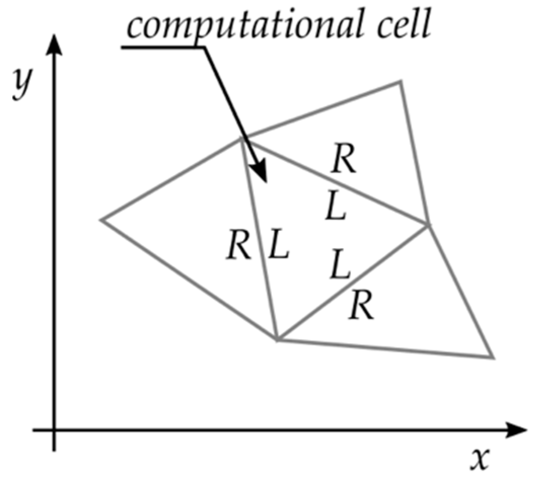
2.1. Mathematical and Numerical Outlines

2.1.1. Advection-Diffusion Model for Large Wood

During high flows, the congested transport of large wood involves the motion of many logs and wooden debris, behaving like a continuum wood carpet that floats on the water surface. The total mass in an infinitesimal planar area dxdy is the product of wood density ρw and the probability density function p(x,θ,t), where the state-space representation includes the planar coordinates x = (x,y) and the planar orientation θ, besides time t. The planar orientation of logs is included since it affects the interaction between logs and with the riverbanks and, consequently, the actual wood mass in the infinitesimal area. More logs fit the same area, if they are aligned with the streamlines, than in cross-flow configuration.
The wood mass continuity equation results in the form of the advection-diffusion equation:
p t + v · p + ω p θ = K x 2 p x 2 + K y 2 p y 2 + K θ 2 p θ 2 + S w ,
where p(x,θ,t) is the probability density function of wood in the space (x,θ), v is the planar transport velocity, ω is the angular velocity, Kx and Ky are the diffusion coefficients in the space (x,y) for anisotropic diffusion, Kθ is the angular diffusion coefficient and Sw represents a source/sink term for the wood probability density function, like a source of mass in the domain that does not affect the flow field, since, as previously stated, wood is considered to be a passive transported substance, one-way coupled with the water flow.
Since two movements occur during wood transport, translation and rotation, the probability density function p(x,θ,t) can be considered to be the product of two distinct contributions:
p ( x , θ , t ) = c w ( x , t )   δ ( x , θ , t ) ,
where cw(x,t) refers to the probability that a wooden element occupies the position x, independently on its orientation, while δ(x,θ,t) gives the probability that a wooden element, positioned in x, has an orientation ranging in (θ,θ + dθ). Substituting Equation (2) into Equation (1) and neglecting the source term Sw, we obtain:
δ c w t + c w δ t + v · ( c w δ ) + ω θ ( c w δ ) = K x 2 x 2 ( c w δ ) + K y 2 y 2 ( c w δ ) + K θ 2 θ 2 ( c w δ ) .
By integrating Equation (3) in the interval (0,2π), being 0 2 π δ ( x , θ , t ) d θ = 1 , due to the flow continuity equation and to the fact that cw(x,t) and v are independent of θ, it results:
c w t + c w v = K x 2 c w x 2 + K y 2 c w y 2 ,
which is the advection-diffusion equation of the positional probability density function.
Finally, multiplying Equation (4) by δ, subtracting it to Equation (3), and dividing the results by cw(x,t), the advection-diffusion equation of the angular probability density function reads:
δ t + v · δ + ω δ θ = K x 2 δ x 2 + K y 2 δ y 2 + K θ 2 δ θ 2 .
At this stage, the main interest is in the transport of wooden mass, since we aim at evaluating the capabilities of the model to replicate wood transport and not the interactions with inline structures. For this reason, the solution of Equation (5) is not considered in this paper, although its implementation is fundamental for future steps and for the simulation of wood accumulation at bridge piers.

2.1.2. Outlines of the Coupled System

To provide an accurate solution of the flow and LW dynamics, the advection-diffusion model for mass probability density function (Equation (4)) is coupled with the solution of the SWE. The coupling is performed following the mathematical model proposed in [33]. Here, for briefness, only the final form of the system of equation that needs to be solved is reported:
U t   +   F ( U ) x   +   G ( U ) y   =   S ( x , y , U ) ,
being,
U   = ( h , q x , q y , h φ ) T , F   = ( q x , q x 2 h + g h 2 2 , q x q y h , u h φ ) T , G   = ( q y , q x q y h , q y 2 h + g h 2 2 , v h φ ) T , S   = ( 0 , g h ( S 0 x     S f x ) , g h ( S 0 y     S f y ) , ¯ ( K h ¯ φ ) ) T ,
where h is the water depth, qx = uh and qy = vh are the unit discharges along the x and y coordinates, u and v are the components of the velocity vector v, along the x and y coordinates, respectively, g is the gravity acceleration, S0 is the source term due to bed slope, Sf is the source term due to friction (expressed with the Manning coefficient), K is the diffusion matrix (diagonal matrix) and φ is the volume averaged wood mass.
The volume averaged wood mass is obtained by multiplying the spatial probability density function cw(x,t) by the wood density ρw and dividing it by the water volume of the computational cell:
φ = c w ρ w h   d x   d y ,
where dxdy represents an ideal planar area.
The numerical model ORSA2D is thus modified to solve the conservative form of Equation (6). ORSA2D is a hydrodynamic model that follows a finite-volume approach, implementing a Roe-Riemann scheme to solve the SWE [34]. It can model both steady and unsteady flow, with proper boundary conditions that can be constant or time dependent. The numerical approach for the coupled solution is essentially the same adopted for the solution of the SWE alone [34], the main difference being the additional unknown included in the new system of Equations (6), which results in an additional eigenvalue and an additional eigenvector, plus one element for the others, of the approximated flux Jacobian.
The details of the numerical model are the same used by [33] in the coupling between SWE and solute flow and are fully described there. Here, we only report the resulting approximated eigenvalues and eigenvectors for the coupled SWE-LW case:
λ ˜ 1   =   u ˜ · n   +   c ˜ , λ ˜ 2   =   u ˜ · n , λ ˜ 3   =   u ˜ · n     c ˜ , λ ˜ 4   =   u ˜ · n ;
e ˜ 1   =   ( 1 u ˜ + c ˜ n x v ˜ + c ˜ n y φ ˜ ) ,                     e ˜ 2   =   ( 0 c ˜ n y c ˜ n x 2 φ ˜ ) ,                     e ˜ 3   =   ( 1 u ˜ c ˜ n x v ˜ c ˜ n y φ ˜ ) ,                     e ˜ 4   =   ( 0 0 0 1 ) .
In Equations (9) and (10), the eigenvalue λ ˜ 4 refers to the wood transport equation, as well as the fourth term of the eigenvectors e ˜ 1 ,   e ˜ 2 ,   e ˜ 3 and the eigenvector e ˜ 4 . The symbols with tilde used in Equations (9) and (10) are the averaged values of the velocity components (u,v), celerity c and wood averaged concentration φ:
u ˜   =   u R h R + u L h L h R + h L   ,                     v ˜   =   v R h R + v L h L h R + h L , c ˜   =   g h R + h L 2   ,                   φ ˜   =   φ R h R + φ L h L h R + h L ,
where the R and L subscripts refer to the considered side of an edge of the computational cell (respectively, right, or outer, and left, or inner, side of the edge, Figure 1).
The boundary conditions for the system of equation Equation (6), considering water, are the standard ones usually included in hydrodynamic models (e.g., water stage or discharge hydrograph, rating curve, Froude number hydrograph [34]).
Regarding wood, a wood mass hydrograph can be set as upstream boundary condition while a simplified condition is proposed for the downstream boundary. The wood concentration at the right side of a boundary edge (φR) is set equal to the total wood concentration of the computational cell, so that the average value computed for calculation (Equation (11)) depends only on the difference between the left and right water depth. Since, for boundary edges, the right water depth hR is calculated from the downstream boundary conditions, the wood mass follows the variations of the water depth that are related to the selected condition.
The diffusion source term in Equation (6) is treated as in [35], integrating it on the computational cell, applying Gauss’s theorem and then discretizing the contour integral with a sum over the cell edges:
Ω i   ¯ ( K h ¯ φ )   d Ω   =   Ω i   ( K h ¯ φ )   n   d s   =   k = 1 N E ( K R + K L 2 n   m i n ( h R , h L ) δ φ d R L ) k n k s k ,
where n is the normal vector of the edge (pointing outside the computational cell), NE is the number of edges, s is the length of each edge, KR and KL are the matrix for anisotropic diffusion, hR and hL are the water depth (predictor values) at each edge side, δφ = (φR − φL) is the difference between the volume averaged wood mass (evaluated with an explicit method) and dRL is the distance between the center of the cells right and left, with respect to the considered edge. R and L subscripts are the same as above.
In addition, to reduce the numerical diffusion observed for the wood mass transport and improve the solution accuracy of the diffusion term also with a first order accurate numerical scheme, a numerical correction was derived from [35]. It involves the computation of a corrective diffusion matrix Kcorr, which is only dependent on the mesh geometry and on the fluid velocity that is subtracted to the diffusion term if it is positive and smaller than it. The correction is calculated for each time step Δt:
K c o r r = 1 2   | u · n |   ( d R L | u · n | Δ t ) ,
and it is implemented as follows:
k = 1 N E ( K   m i n ( h R , h L ) δ ϕ d R L ) k s k ,
with
{ K = 0 i f   K c o r r > ( K R + K L 2 ) k n k n k K = m a x ( ( K R + K L 2 ) k n k n k K c o r r , 0 ) i f   K c o r r ( K R + K L 2 ) k n k n k
Finally, the time step is calculated considering both the Peclet and the Courant-Friedrichs-Lewy (CFL) numbers, limiting the value to further reduce diffusivity problems [35].
The diffusion coefficients of the matrices KR and KL are derived from the results presented in [30], in which streamwise and transversal coefficients (Ks, Kt) were provided as a function of the particle Froude number Frp and of the transversal relative release distance tRr of the mass concentration (Equation (16)). These values are combined according to the local velocity orientation to obtain the elements of the diffusion matrices (Equation (17)).
K s   =   0.005   ( F r p ) 0.740 ( t R r ) 0.300 ,     K t =   0.011   ( F r p ) 0.188 ( t R r ) 0.271 ;
K x x   =   K s u + K t v u 2 + v 2 , K y y   =   K s v + K t u u 2 + v 2 , K x y   =   1 2 ( K s K t ) 2 u v u 2 + v 2 ;
where F r p   =   v M A X g L w , t R r   =   t R L W , Lw is the length of the wood pieces, tR is the release distance from the right bank, u and v are the flow velocity component, Kxx and Kyy are the diagonal element of the diffusion matrix and Kxy the off-diagonal elements.

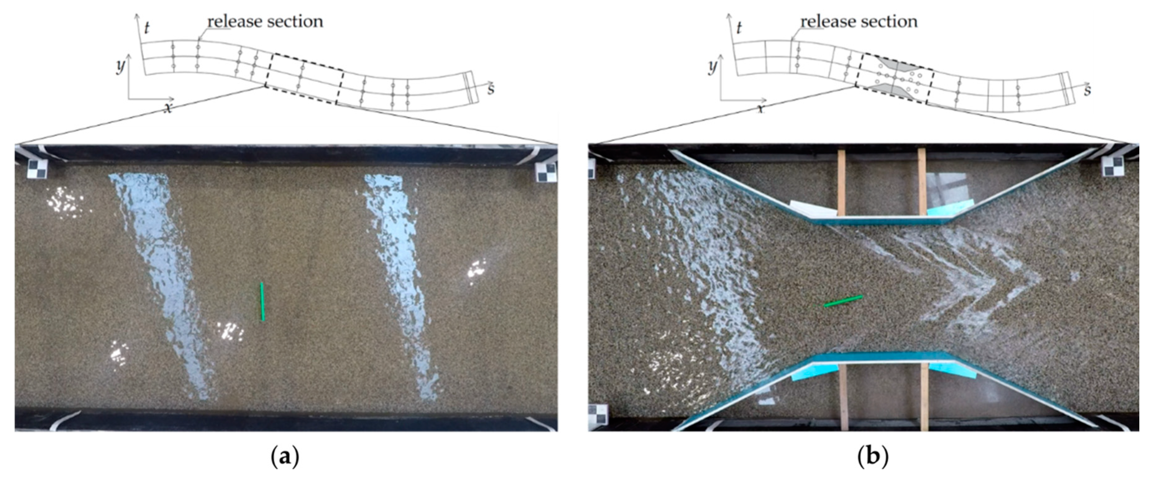
2.2. Experiments Description

The numerical model is tested on a series of flume experiments performed at the University of Trento, described in [30]. Here the main aspects relevant to the comparison with the numerical results are reported.
Two flume configurations were employed: a S-shaped flume and a S-shaped flume with a gradual Venturi narrowing that halves the flume section. In the first case, the bottom slope was also varied. The flumes are 2 m wide, with a reduction to 1 m in the narrowing, and about 22 m long, with rectangular section, vertical side walls (1 m high) and a fixed gravel bed (D50 = 8 mm).
The experiments were performed in steady flow conditions, releasing logs one by one and filming their trajectories with 3 GoPRO Hero 5 cams, located 2.5 m above the flume (30 fps, pixel resolution 1920 × 1080, linear Field Of Vision), able to frame altogether nearly the entire length of the flume. Figure 2 shows the flume planar views and a frame from the central camera.
Through data analysis [30] each log trajectory was estimated, acquiring time, planar positioning, and orientation. Cylindrical logs, smooth and varnished with green impermeable painting, were employed. Lengths and diameters were selected based on a theoretical physical scale (λh = 60 and λh = 40, horizontal and vertical, respectively). The cylinders average density is 790 kg m−3, such as that of green wood broadleaved trees [36].
Table 1 resumes the characteristics of the experiments used as a reference for the numerical model. The main parameters relevant to the experimental analysis and numerical simulation are the flow Froude number F r = v m e a n g h , which remains constant only for the S-shaped flume, the transversal position of release (calculated from the right sidewall) tR, the log length Lw and diameter Dw.
The flow velocity was measured with an Acoustic Doppler Velocimeter for each hydraulic condition, in the points shown in circles in Figure 2.

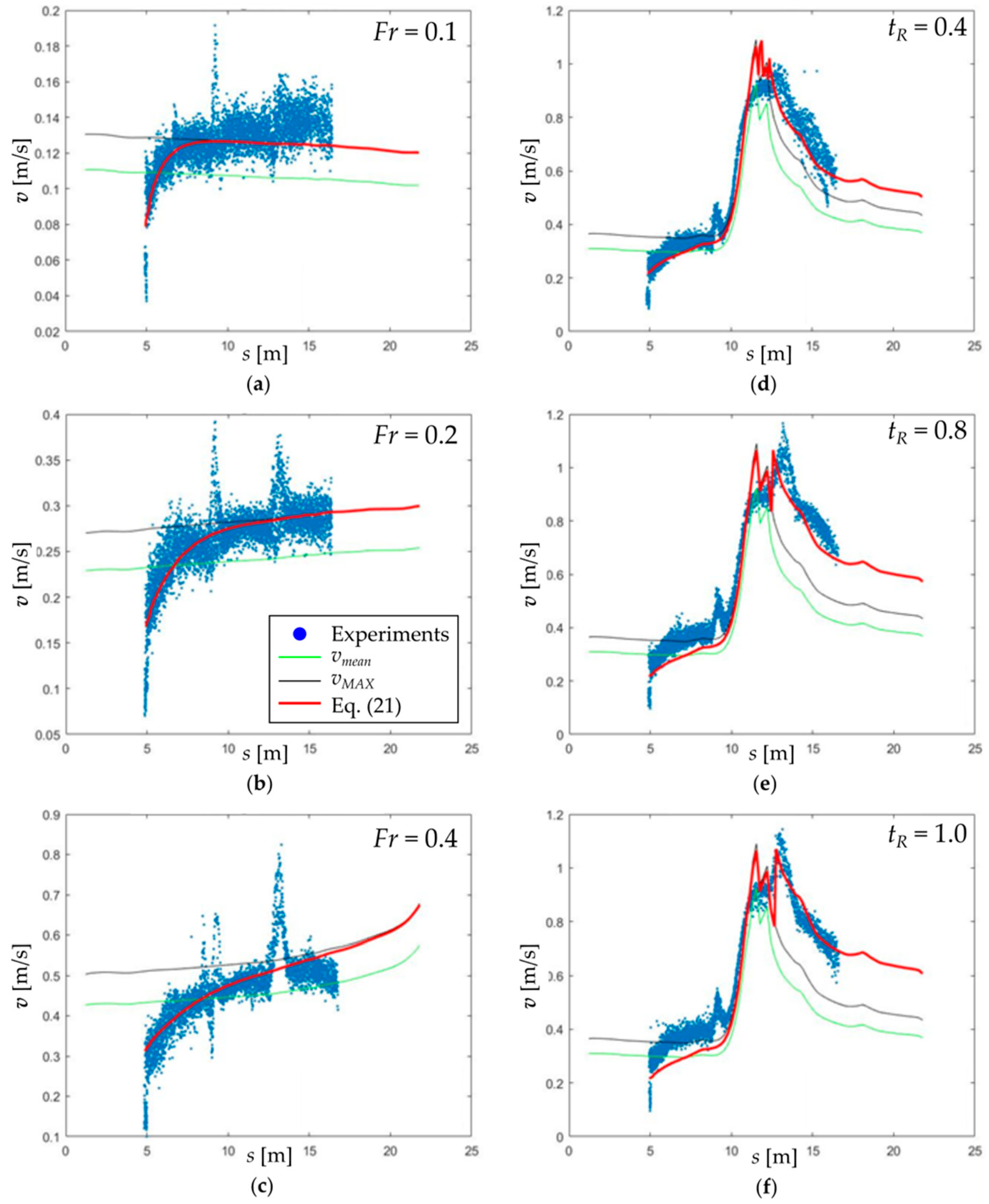
2.3. Modeling the Transport Velocity

In the considered experiments, and in most cases in the natural environment, wood density is lower than the water density [30], so wood logs float on the water surface and are transported by the superficial flow. Under such conditions, the vertical averaged mean velocity, computed by the SWE model, is not representative of the actual transport velocity v of the advection-diffusion model (Equation (4)). This velocity is more likely to be the maximum flow velocity, computed as a function of the mean value assuming, for example, a (1/7)th power velocity distribution:
v M A X   =   1 0.85   v m e a n .
In addition, when a log is entrained in the flow, its initial velocity is lower and tends to adapt to the surface flow velocity. The same behavior was observed in the experiments described in Section 2.2, which presented a velocity near to 0 m s−1 at the beginning due to the permanence in the release device. In [30], an asymptotical formulation is proposed based on the analysis of a single test case (Fr = 0.4, LW = 0.20 m, DW = 0.02 m, tR = 0.80 m). To generalize that formulation, a non-dimensional coefficient cvel is obtained:
c v e l   =   ( 0.3 + 0.19 ( 1 e t c ) ) 1.18 0.49 ,
that can be multiplied by the mean flow velocity of each computation cell containing wood mass concentration to estimate the actual transport velocity (v = cvel vmean). The value c at the exponent denominator is linearly correlated with the Froude number FrR, evaluated at the release point, and its expression is:
c = 4.39 F r R .
Logs velocity estimation in the S-shaped flume with narrowing showed that just downstream of the narrowing, the logs tend to maintain a velocity higher than the theoretical one (computed with the asymptotical formulation). This probably occurs because of the log inertia that delays the adaptation of the log velocity in case of sudden flow deceleration, especially in presence of section variation, energy loss and turbulent flow behavior. An additional coefficient is thus included in the proposed model to increase wood velocity in case of local and abrupt decelerations, i.e., when the maximum wood concentration undergoes a velocity reduction greater than a threshold value based on the experiments. This coefficient is related to the release transversal position tR: if the logs are nearer to the flume sidewalls, they are subject to higher gradients that tend to diminish their velocity, while if they flow nearer to the flume axis, they maintain a higher velocity. The deceleration coefficient kd is thus defined as follows:
k d = 1 + 0.4 t R .
Overall, the transport velocity computed at each time step, for each cell i containing a wood concentration, is:
{ v ( i , t ) = ( 0.3 + 0.19 ( 1 e t c ) ) 1.18 0.49   i f   v f ( i c   m a x , t ) v f ( i c   m a x , t 1 ) > Δ v v ( i , t ) = ( 0.3 + 0.19 ( 1 e t c ) ) 1.18 0.49 k d i f   v f ( i c   m a x , t ) v f ( i c   m a x , t 1 ) Δ v ,
where FrR is the Froude number at the release point, vf is the flow velocity computed by ORSA2D, ic max is the cell where the maximum concentration is found at the considered time instant and Δv is a threshold value (Δv = −0.16 m s−1 based on the experimental tests).
The transport velocity resulting from Equation (22) is shown in Figure 3, compared with the experimental log velocity, with the mean flow velocity computed by ORSA2D and with the maximum theoretical flow velocity obtained by applying Equation (18).

2.4. Details of the Numerical Tests

The experiments described in Section 2.2 are simulated with ORSA2D model modified to simulate wood mass advection-diffusion. Both the S-shaped flume and the S-shaped flume with narrowing are discretized with triangular cells of about 0.05 m side, for a total number of 39,856 elements for the first, and 38,256 for latter (which presents fewer elements since the narrowing is treated as a solid physical boundary, see Figure 4).
The inlet discharge, set as upstream boundary condition, and the bottom slope are shown in Table 1. The roughness is represented with a constant Manning coefficient, n = 0.021 s m−1/3, while the imposed downstream boundary condition is the downstream Froude number, set equal to 0.09, 0.25 and 1 for the three tests in the S-shaped flume, and 0.36 for the flume with narrowing. While the latter was estimated from experimental measures, the first three were calibrated to reduce the differences between the experimental and the numerical flow velocities.
The wood mass is assumed to be released in a single cell, corresponding to the mean initial position of the logs for each test, with a triangular wave function. Equation (23) shows the computation of the input concentration rate:
φ ( x , t ) t = ρ w i = 1 N L L w i D w i 2 4 π A c e l l h c e l l T r e f
where the numerator represents the total mass for the considered experiment (NL being the number of repetitions, or of total logs released, as in Table 1) while the denominator includes the input cell area, Acell, water depth hcell and the estimated release duration Tref. The release duration is set equal to 1.2 s and was evaluated based on the actual release time observed during the experiments performed for the experimental campaign of [32].

3. Results

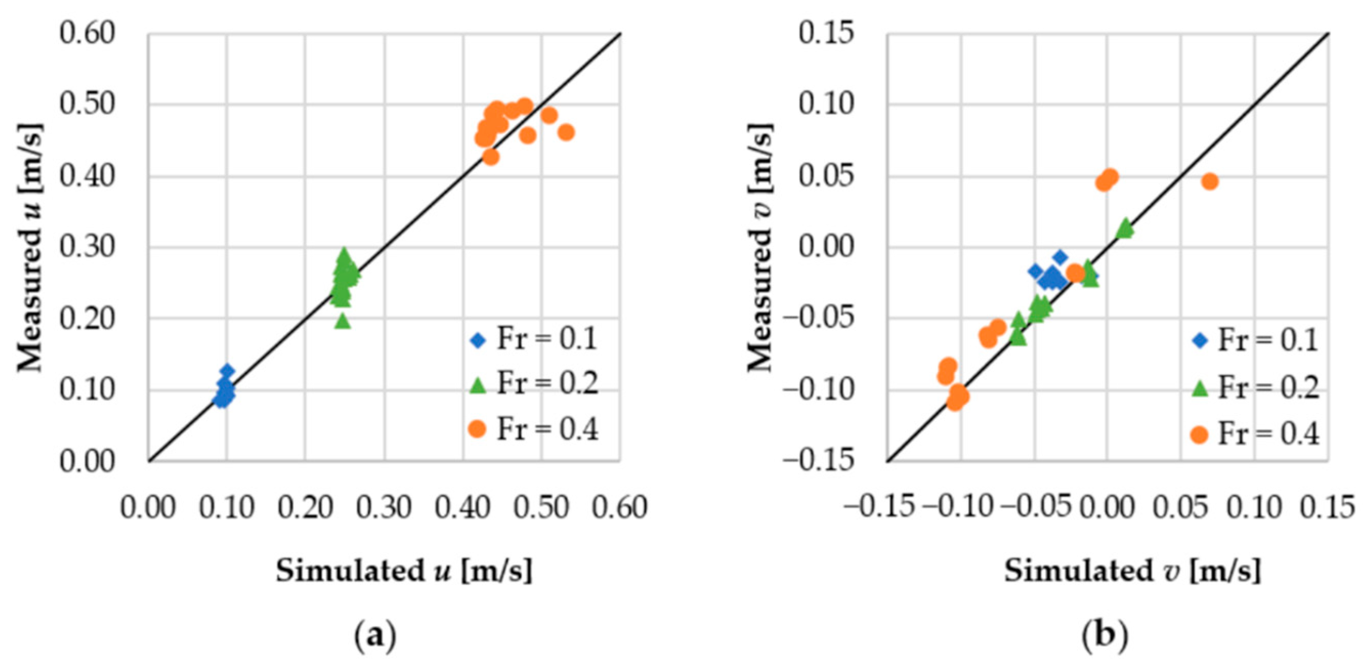
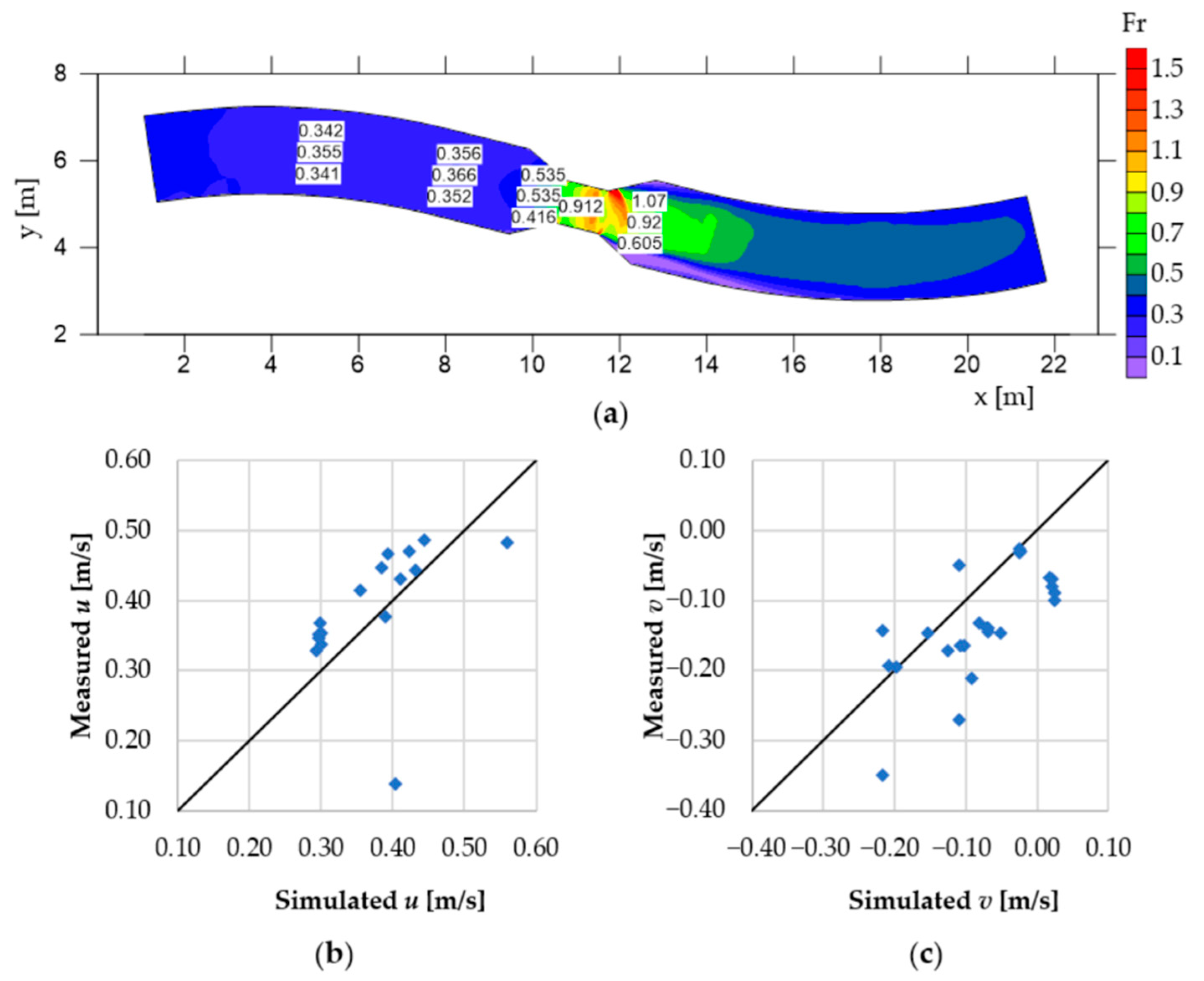
3.1. Hydraulic Simulation

Numerical results are compared with the available measures (velocity measures in the points shown in Figure 2) to provide an evaluation of the simulation accuracy. Water depth was not measured for the S-shaped flume, so the local Fr was not computed.
Regarding the S-shaped flume (Figure 5), a good agreement is observed for the measured and simulated velocities. Better correlation is observed for the v component (Figure 5b, average correlation coefficient R2 = 0.71) than for u component (Figure 5a, average correlation coefficient R2 = 0.20), which is less variable in the simulation than in the experiments (especially for the lower Froude numbers).
Figure 6a shows the computed and measured Froude number along the S-shaped flume with narrowing, while Figure 6b,c show the comparison of the flow velocity. The correlation coefficients are 0.79 for the Froude number, 0.77 for the u component and 0.69 for the v component, confirming the good representation of the flow in this flume. Most likely, the fact that the downstream boundary condition was based on experimental measures affected the higher quality of the numerical simulation, compared with the test in the S-shaped flume.

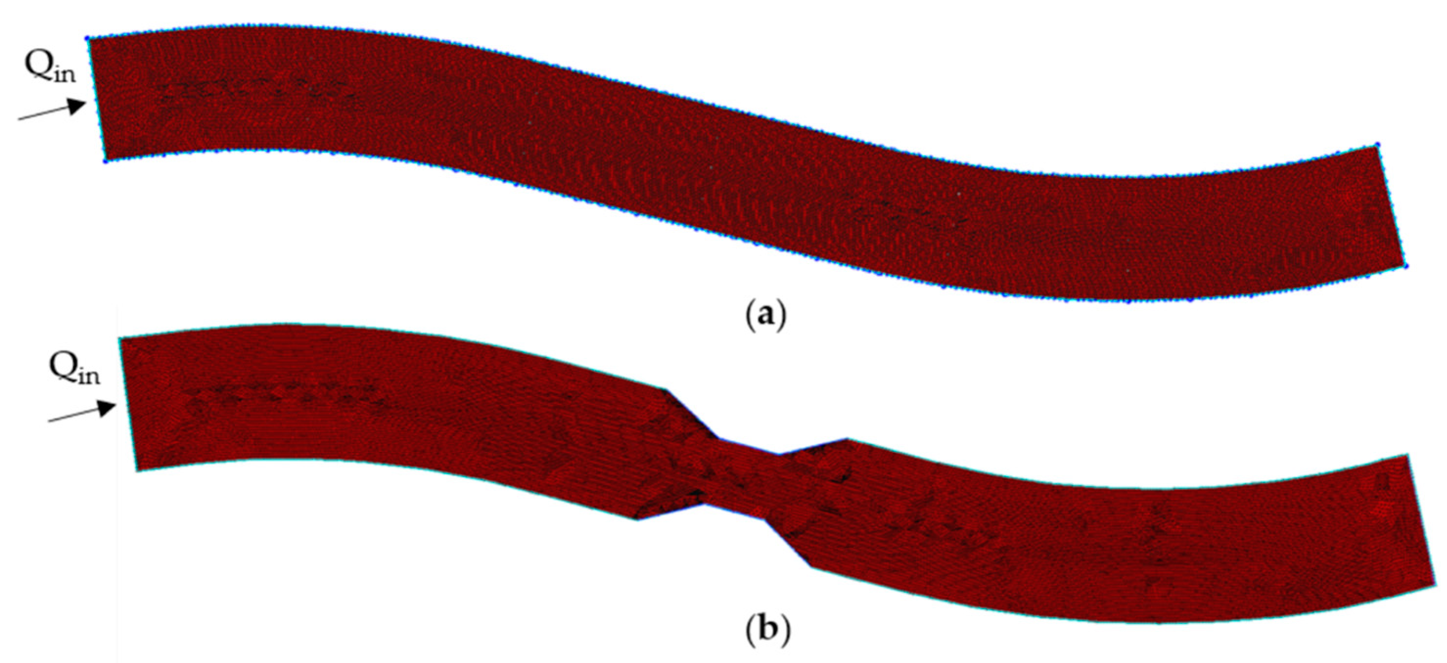
3.2. Wood Transport Simulation

The wood transport simulations are carried out from steady state hydraulic conditions. The wood concentration is released at 50 s, which is then considered to be the initial time for wood transport. As shown in Table 1, several tests were modeled that differ for the main parameters affecting diffusion: flow Froude number, log length Lw, log diameter Dw and release distance tR from the right side of the channel.
For each hydraulic condition examined in the previous section, the results of selected tests are presented, at regular time intervals and at the last available instant, while in the discussion paragraph a synoptic comparison will be shown. Please note that in the experiments each log was separately released, following its own trajectory, and not interacting with the others. Grouped representations have the sole purpose to help the distribution visualization and results discussion.

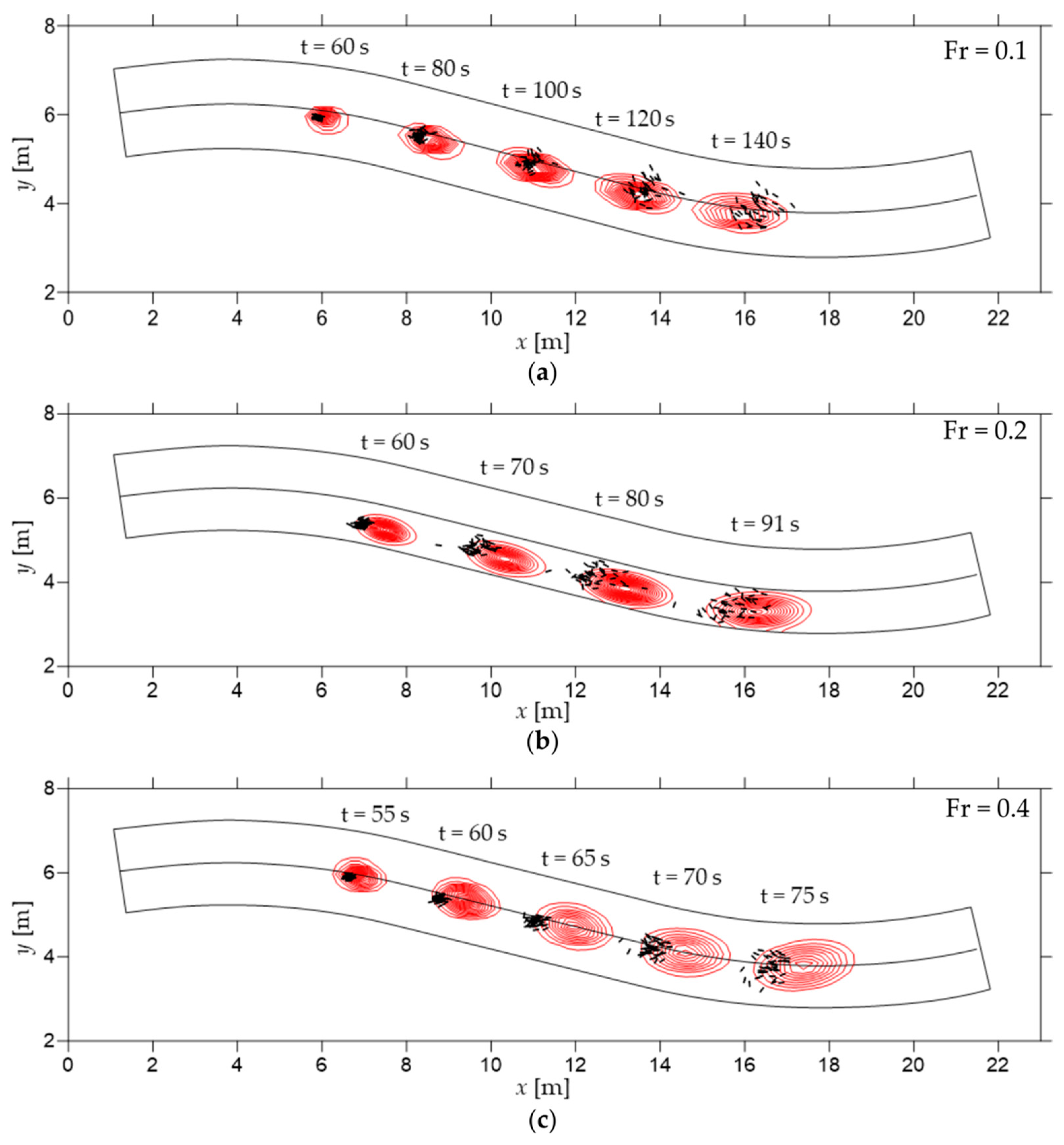
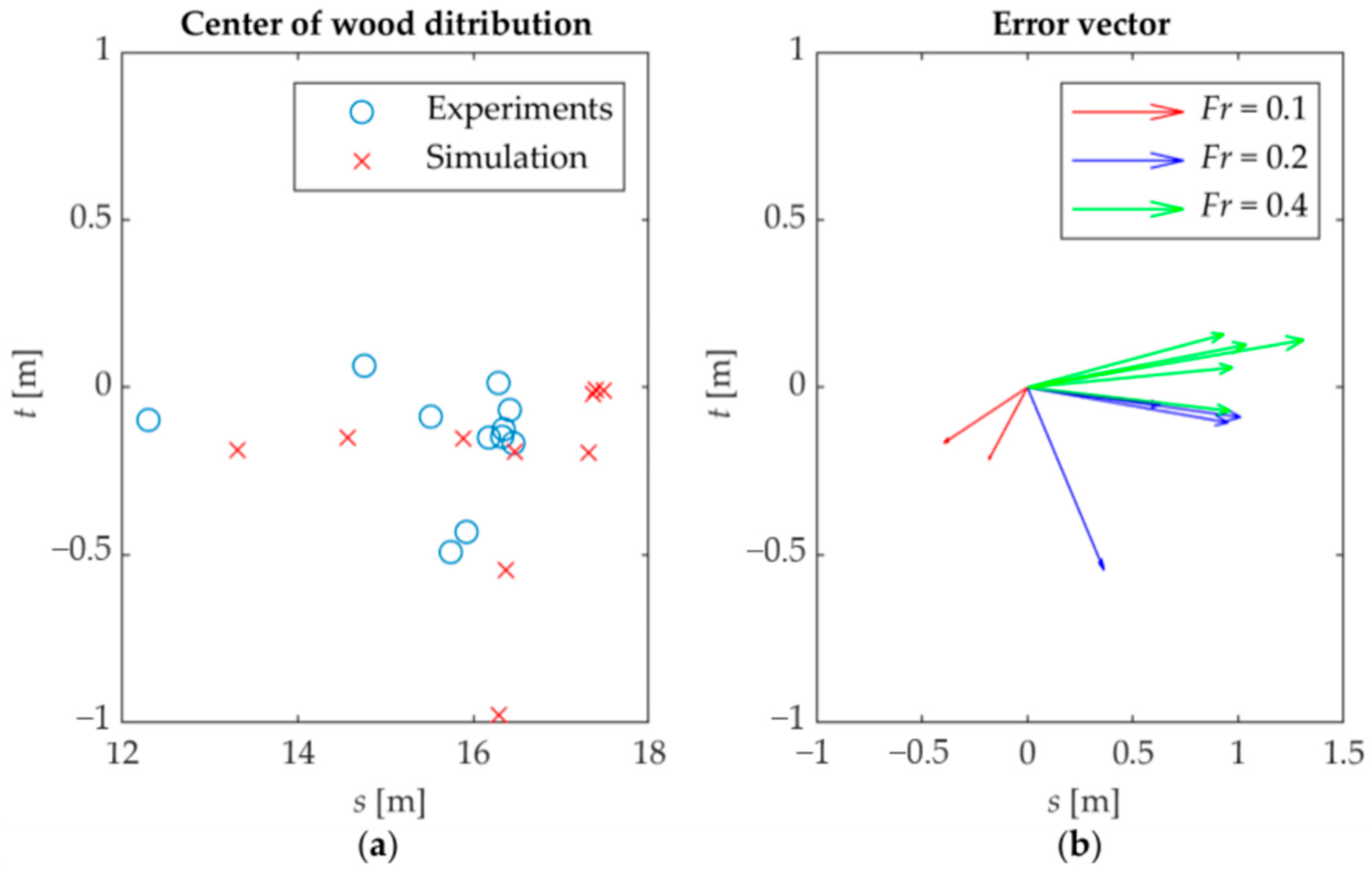
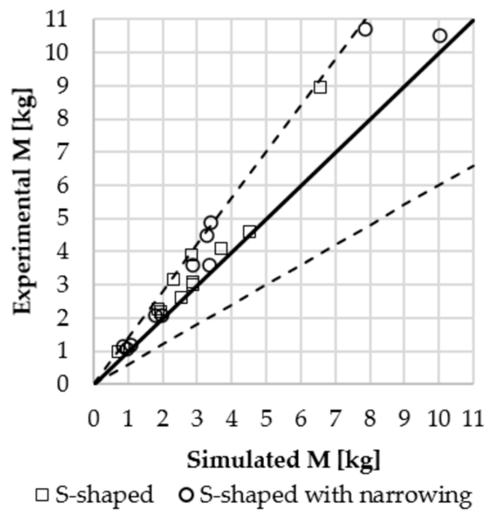
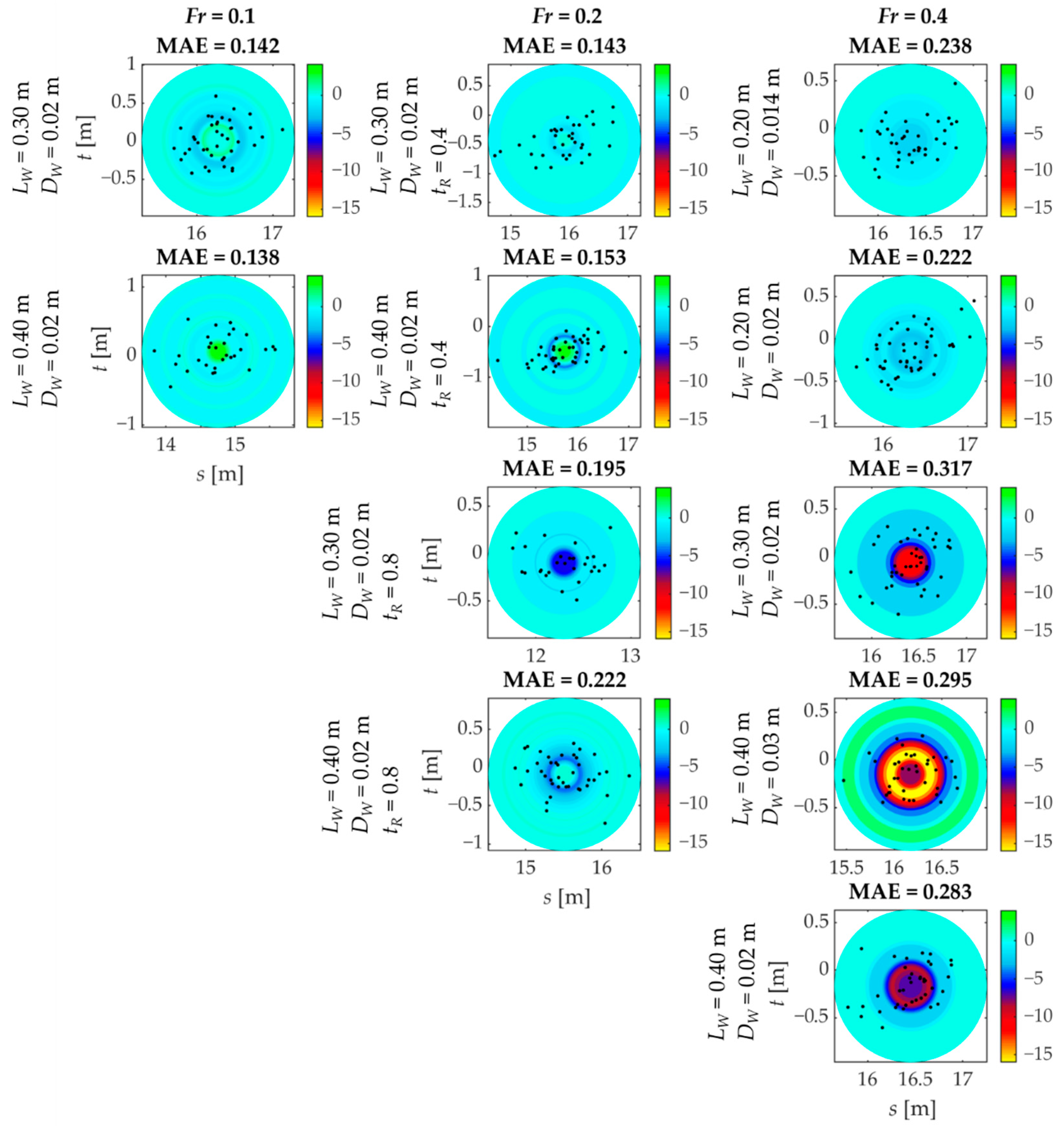
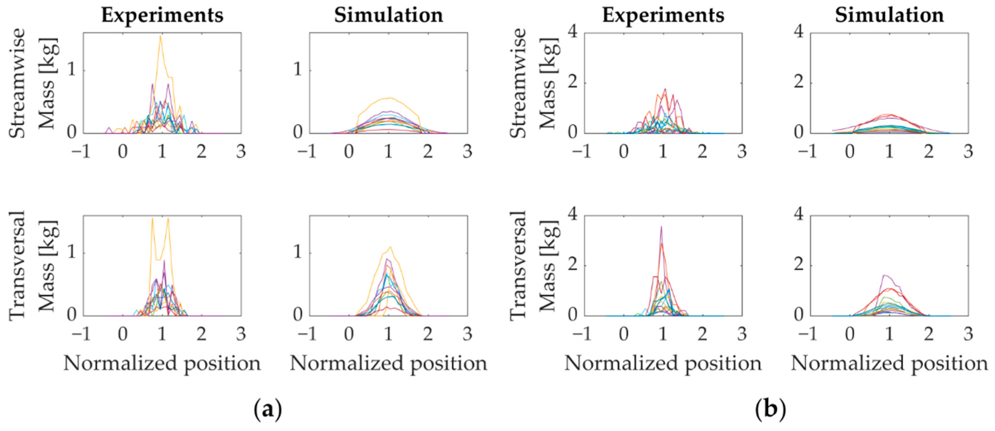
3.2.1. S-Shaped Flume

Graphs in Figure 7 show the comparison of the experimental log position and the computed wood concentration for three tests in the S-shaped flume, with different flow conditions. In each sub-figure, a time sequence is shown, with a time interval of about 20 s, 10 s and 5 s, shorter for the test with higher Froude number. The minimum value of the volume averaged concentration that corresponds to the largest contour line, is 5 kg m−3 and the last time instant varies depending on the considered test (140 s, 91 s and 75 s for the shown graphs).

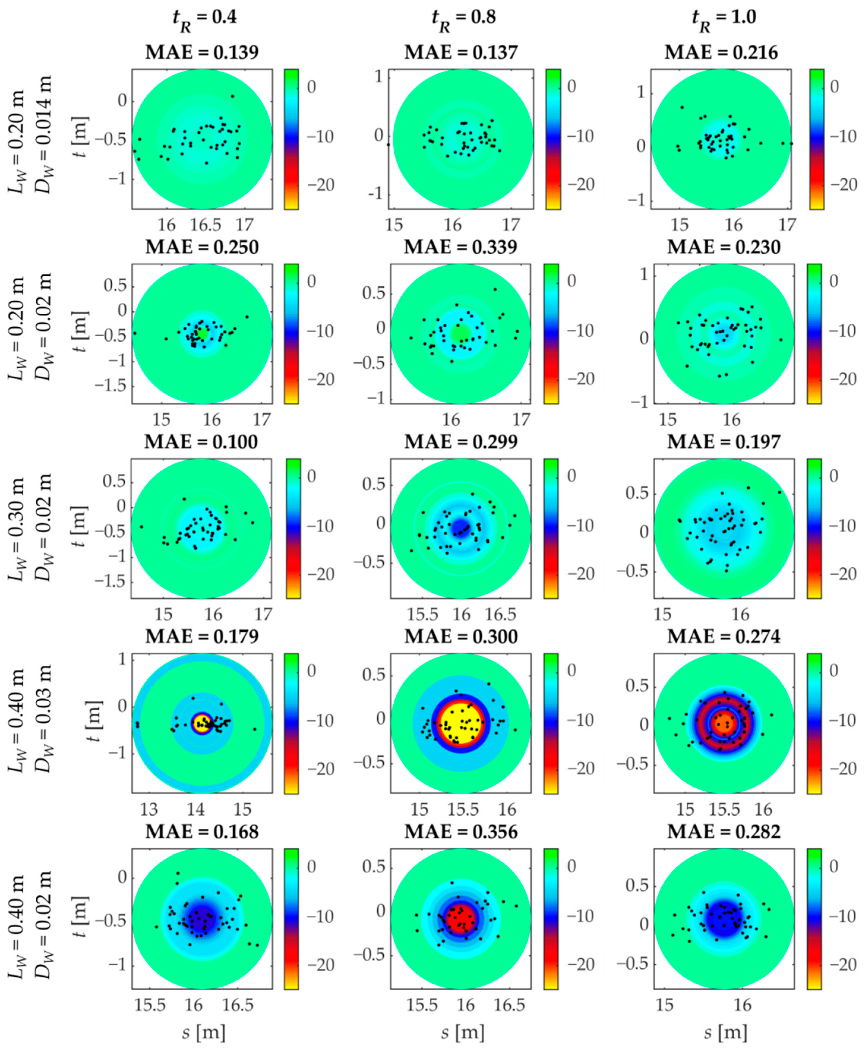
3.2.2. S-Shaped Channel with Venturi Narrowing

Graphs in Figure 8 show the comparison of the experimental log position and the computed wood concentration for three tests with different release distance from the right bank, in the flume with the narrowing. The time sequence has an interval of 5 s and the minimum value of the volume averaged concentration that corresponds to the largest contour line, is 5 kg m−3. The final time, which will be considered to be a reference time for the discussion, varies slightly for each test (71 s, 72 s and 74 s).

4. Discussion

Figure 7 and Figure 8 show how the wood is transported in the experimental tests. It must be highlighted that despite the experiments were performed releasing the logs one by one [30], in these figures they are shown altogether as black segments, to better visualize their distribution. In general, logs are grouped at the initial time, since they are released in the same position, and then spread longitudinally and transversally because of flow advection and surface turbulent diffusion.
Similarly, the numerical results are concentrated at the initial time and tend to expand while flowing downstream. In all the simulations, the planar enlargement of the area of non-zero concentration (red contours in Figure 7 and Figure 8) appears to be wider than the scattering of the experimental logs, although the outer contour line represents a very low volume averaged concentration (5 kg m−3) that for the volume of an average cell, corresponds to a wood mass lower than 1 g.
For the S-shaped flume (Figure 7), the peak of the numerical concentration often moves downstream faster than the experimental logs, as it can be viewed by the center of the contour lines being located downstream of the center of mass of the groups of logs in the experiments. The opposite happens in case of constriction (Figure 8), where at each time step, a better agreement between the area occupied by the logs and by the numerical contour lines is found.
To provide a synoptic evaluation of the model, a comparison between the experimental concentration and the numerical tests at the final time instant is considered. The time is selected as the maximum time at which all the logs released in the flume (NL) are visible in the recording (e.g., the final time shown in the Figure 7 and Figure 8, but it varies for each test).
To analyze the accuracy of the simulation, the location of the mean position of the experimental logs is compared with the location of the cell with the maximum concentration (i.e., the most probable position) in the simulation. Figure 9a and Figure 10a show that the mean planar position for each test is, on average, in the range 14.5–16.5 m in the streamwise direction for the S-shaped flume and 15.5–16.5 m for the flume with narrowing (with one exception for both configurations). Average transversal positions are grouped around the flume axis (+0.2 m, −0.6 m). The numerical maximum, observed at the same time selected for the experiments, is scattered longitudinally for the S-shaped flume (13–17.5 m), while it is well grouped for the flume with narrowing, although in a lower range of streamwise coordinates (14.75–16 m). In both cases, the transversal ranges are like the experimental ones.
The differences found for the two flume configurations are confirmed by Figure 9b and Figure 10b, which show the distance vector between the numerical and experimental average positions, giving a visual representation of the error in estimating the most probable position of the transported logs. For the S-shaped flume (Figure 9b), in most cases these vectors point in the downstream direction, showing that the numerical concentration tends to flow faster than experimental logs. On the contrary, the numerical concentration is slower in the flume with narrowing, with vectors pointing upstream (Figure 10b). Considering both flumes, the global mean absolute percentage error is 4.5% and 16.5% for the streamwise and transversal coordinates, respectively.
Up to now the focus was on the log mean position, or most probable location of the maximum concentration. An additional validation can be performed by checking if the model can distribute the mass as observed in the experiments.
For this purpose, a “target area” is identified, as a series of concentric rings, which are centered on the log mean position for the experiments and on the coordinates of the cell with the maximum concentration for the simulations. The rings are 0.05 m wide and the maximum diameter is set to include the maximum span of the log positioning (which may differ for each test).
For the experiments, the concentration is computed by dividing the total mass in each ring (number of logs inside the ring times log volume times wood density, M = N i n   r i n g L W D W 2 4 ρ W ) by the ring planar area. The value obtained is the planar concentration of wood mass, named “experimental concentration” hereafter. For the numerical simulations, the total concentration in each ring is the sum of the concentration of each domain cell that is included in that concentric ring.
The total mass in the target area is shown in Figure 11. For both the flumes, the simulated mass corresponds to the experimental one within a confidence interval of 40%. In all cases, the total simulated mass is equal or lower than the experimental one. Please note that the total mass at the end of each simulation is equal to the released mass, so the reduction observed in Figure 11 is related to the dimension of the target area, which is too small to comprise the total concentration. The extension of the target area, in fact, is set upon the experimental planar distribution, which is clearly reduced with respect to the numerical one (e.g., see Figure 7 and Figure 8). Independently of the flume configuration, the lowest accuracy is obtained for the experiments with the largest mass involved (i.e., wooden samples with LW = 0.4 m and DW = 0.03 m). On average, the numerical wooden mass included in the target area is about 85% of the experimental one.
Figure 12 and Figure 13 show the difference of the numerical concentration minus the experimental one, in each ring. In most cases the largest differences are in the inner rings, with the numerical values being lower than the experimental ones for both flume configurations. Once again, the simulations diffuse the mass concentration more than expected, with lower values in the central rings and a concentration distributed on an area wider than the target one.
The position of the centers of mass of the logs in the experiments, shown as black dots in all the graphs of Figure 12 and Figure 13, confirms that the logs are not evenly distributed in the circular areas but present, in general, a longitudinal dispersion higher than the transversal one, which is more or less evident depending on the considered test. On the contrary, the numerical results are more gradually distributed. As well as for the total mass estimation, the largest differences are observed for the tests involving the longer logs, so the greater mass.
A quantitative evaluation of the difference of the distributed planar concentration is computed with the Mean Absolute Error (MAE = |exp.conc. − num.conc.|, valuated for each concentric ring), which has a global average value of 0.22 kg m−2.
Finally, the wood mass distribution along the two main diameters of the target area (in streamwise and transversal direction) is shown in Figure 14. All the lines are centered on the position of the maximum mass, in the streamwise or transversal direction, and the slot amplitude to calculate the mass in each spatial interval (either sum of the logs mass or sum of the mass in the cells) is of 0.05 m. The maximum width of the graphs corresponds to the maximum radius of the target area.
Figure 14 confirms that independently of the flume shape, the experimental mass is strongly concentrated around the mean position, in both directions, with a larger dispersion in the streamwise direction. Experimental mass is discontinuously distributed, while the simulated results appear smoother. In this case, the mass is gradually distributed along the two directions and the maximum values are underestimated, especially for the streamwise direction.
This suggests that the model provides an acceptable simulation of the transversal diffusion, while the longitudinal one is overestimated.

5. Conclusions

A Eulerian model for the simulation of congested large wood transport is here proposed. It allows the one-way coupled solution of the Shallow Water Equations for the flow and the advection-diffusion equation for wood mass concentration, including proper modification to consider the floating transport. In fact, the transport velocity is expressed with an asymptotic formulation, able to mimic the inertia of large wood to the flow accelerations and decelerations, and the diffusion model comprise ad hoc diffusion coefficients.
The application of this model to a series of experiments shows a good agreement between numerical and experimental results. The model can predict the evolution of the transported wood mass and the most probable location of wood, with a percentage error of 4.5% and 16% in the streamwise and transversal directions.
Nonetheless, the diffusion appears greater than expected, with an underestimation of the maximum concentration and a consequent wider planar distribution of wood mass. This may depend on some overestimation of the diffusion coefficients or, more probably, on a numerical diffusion that remains high despite the implemented correction. An in-depth analysis of the numerical diffusion tensor, comprising also different discretization methods (like finite element, e.g., [37,38]) may help assessing the actual role of the numerical diffusivity for the proposed scheme.
Overall, the model results are promising, but additional investigation is required to fix issues connected with diffusion. Additionally, since real events may include fine wood among larger wooden elements, the model behavior under such conditions should be also investigated. Finally, it would be advisable to include the effect of Large wood orientation that is a significant parameter for the application to real cases, since it affects the probability of accumulation and the consequent backwater effect.

Author Contributions

Conceptualization, S.S., G.P. and A.A.; methodology, G.P., S.S., A.A. and E.P.; software, G.P., E.P. and R.B.; validation, E.P. and R.B.; data curation, E.P. and R.B.; writing—original draft preparation, E.P. and R.B.; writing—review and editing, E.P., G.P., S.S., R.B., A.A. All authors have read and agreed to the published version of the manuscript.

Funding

This research received no external funding.

Acknowledgments

The authors thank Sabrina Meninno and Elena Nucci for experimental data sharing. Thanks to anonymous reviewers for their comments and suggestions which helped in improving the quality of the paper.

Conflicts of Interest

The authors declare no conflict of interest.

References

  1. Mačiukėnaitė, J.; Povilaitienė, I. The role of the river in the city centre and its identity. J. Sustain. Archit. Civ. Eng. 2013, 4, 33–41. [Google Scholar] [CrossRef] [Green Version]
  2. Costabile, P.; Macchione, F.; Natale, L.; Petaccia, G. Comparison of scenarios with and without bridges and analysis of backwater effect in 1-D and 2-D river flood modeling. Comput. Model. Eng. Sci. 2015, 109, 81–103. [Google Scholar] [CrossRef]
  3. Du, S.; Shi, P.; Van Rompaey, A.; Wen, J. Quantifying the impact of impervious surface location on flood peak discharge in urban areas. Nat. Hazards 2015, 76, 1457–1471. [Google Scholar] [CrossRef]
  4. Blöschl, G.; Hall, J.; Viglione, A.; Perdigão, R.A.; Parajka, J.; Merz, B.; Boháč, M. Changing climate both increases and decreases European river floods. Nature 2019, 573, 108–111. [Google Scholar] [CrossRef]
  5. Xu, H.; Luo, Y. Climate change and its impacts on river discharge in two climate regions in China. Hydrol. Earth Syst. Sci. 2015, 19, 4609. [Google Scholar] [CrossRef] [Green Version]
  6. Llasat, M.C.; Barrera, A.; Altava-Ortiz, V. Floods evolution in a Climate Change framework: A Mediterranean analysis. In Proceedings of the Third International Conference on Climate and Water, Helsinki, Finland, 3–6 September 2007. [Google Scholar] [CrossRef] [Green Version]
  7. Winsemius, H.C.; Van Beek, L.P.H.; Jongman, B.; Ward, P.J.; Bouwman, A. A framework for global river flood risk assessments. Hydrol. Earth Syst. Sci. 2013, 17, 1871–1892. [Google Scholar] [CrossRef] [Green Version]
  8. Macchione, F.; Costabile, P.; Costanzo, C.; De Santis, R. Moving to 3-D flood hazard maps for enhancing risk communication. Environ. Model. Softw. 2019, 111, 510–522. [Google Scholar] [CrossRef]
  9. Hagemeier-Klose, M.; Wagner, K. Evaluation of flood hazard maps in print and web mapping services as information tools in flood risk communication. Nat. Hazards Earth Syst. Sci. 2009, 9. [Google Scholar] [CrossRef]
  10. Nogherotto, R.; Fantini, A.; Raffaele, F.; Di Sante, F.; Dottori, F.; Coppola, E.; Giorgi, F. An integrated hydrological and hydraulic modelling approach for the flood risk assessment over Po river basin. Nat. Hazard Earth Syst. Discuss. 2019, 1–22. [Google Scholar] [CrossRef]
  11. Lucía, A.; Comiti, F.; Borga, M.; Cavalli, M.; Marchi, L. Dynamics of large wood during a flash flood in two mountain catchments. Nat. Hazards Earth Syst. Sci. 2015, 15, 1741. [Google Scholar] [CrossRef] [Green Version]
  12. Comiti, F.; Mao, L.; Preciso, E.; Picco, L.; Marchi, L.; Borg, M. Large wood and flash floods: Evidence from the 2007 event in the Davča basin (Slovenia). WIT Trans. Eng. Sci. 2008, 60, 173–182. [Google Scholar] [CrossRef] [Green Version]
  13. Prima Cremona. Available online: https://primacremona.it/cronaca/crolla-ponte-pedonale-sulladda-a-pizzighettone/ (accessed on 29 September 2020).
  14. Il Dolomiti. Available online: https://www.ildolomiti.it/cronaca/2020/foto-e-video-spaventa-ladige-suona-la-sirena-inizia-levacuazione-a-egna-a-san-michele-preoccupa-il-ponte-ferroviario (accessed on 29 September 2020).
  15. YouTube. Available online: https://www.youtube.com/watch?v=M9SLR6EIN58 (accessed on 29 September 2020).
  16. Braudrick, C.A.; Grant, G.E. When do logs move in rivers? Water Resour. Res. 2000, 36, 571–583. [Google Scholar] [CrossRef] [Green Version]
  17. Alonso, C.V. Transport mechanics of stream-borne logs. In Riparian Vegetation and Fluvial Geomorphology; Bennett, S.J., Simon, A., Eds.; American Geophysical Union: Washington, DC, USA, 2004; Volume 8, pp. 59–69. [Google Scholar] [CrossRef]
  18. Stockstill, R.L.; Daly, S.F.; Hopkins, M.A. Modeling folating objects at river structures. J. Hydraul. Eng. 2009, 135, 403–414. [Google Scholar] [CrossRef]
  19. Persi, E.; Petaccia, G.; Sibilla, S.; Brufau, P.; García-Navarro, P. Calibration of a dynamic Eulerian-Lagrangian model for the computation of wood cylinders transport in shallow water flow. J. Hydroinform. 2019, 21, 164–179. [Google Scholar] [CrossRef]
  20. Kang, T.; Kimura, I.; Shimizu, Y. Numerical simulation of large wood deposition patterns and responses of bed morphology in a braided river using large wood dynamics model. Earth Surf. Proc. Landf. 2020, 45, 962–977. [Google Scholar] [CrossRef]
  21. Gippel, C.J.; O’Neill, I.C.; Finlayson, B.L.; Schnatz, I.N.G.O. Hydraulic guidelines for the re-introduction and management of large woody debris in lowland rivers. Regul. Rivers Res. Manag. 1996, 12, 223–236. [Google Scholar] [CrossRef]
  22. Hygelund, B.; Manga, M. Field measurements of drag coefficients for model large woody debris. Geomorphology 2003, 51, 175–185. [Google Scholar] [CrossRef]
  23. Ruiz-Villanueva, V.; Bladé, E.; Sánchez-Juny, M.; Marti-Cardona, B.; Díez-Herrero, A.; Bodoque, J.M. Two-dimensional numerical modeling of wood transport. J. Hydroinform. 2014, 16, 1077–1096. [Google Scholar] [CrossRef]
  24. Kimura, I.; Kitazono, K. Effects of the driftwood Richardson number and applicability of a 3D–2D model to heavy wood jamming around obstacles. Environ. Fluid Mech. 2020, 20, 503–525. [Google Scholar] [CrossRef]
  25. Persi, E.; Petaccia, G.; Sibilla, S.; Brufau, P.; García-Palacin, J.I. Experimental dataset and numerical simulation of floating bodies transport in open-channel flow. J. Hydroinform. 2020, 22, 1161–1181. [Google Scholar] [CrossRef]
  26. Persi, E.; Petaccia, G.; Sibilla, S.; Lucia, A.; Andreoli, A.; Comiti, F. Numerical modelling of uncongested wood transport in the Rienz river. Environ. Fluid Mech. 2020, 20, 539–558. [Google Scholar] [CrossRef]
  27. Ruiz-Villanueva, V.; Bodoque, J.M.; Díez-Herrero, A.; Eguibar, M.A.; Pardo-Igúzquiza, E. Reconstruction of a flash flood with large wood transport and its influence on hazard patterns in an ungauged mountain basin. Hydrol. Process. 2013, 27, 3424–3437. [Google Scholar] [CrossRef]
  28. Ruiz-Villanueva, V.; Bodoque, J.M.; Díez-Herrero, A.; Bladé, E. Large wood transport as significant influence on flood risk in a mountain village. Nat. Hazards 2014, 74, 967–987. [Google Scholar] [CrossRef] [Green Version]
  29. Braudrick, C.A.; Grant, G.E.; Ishikawa, Y.; Ikeda, H. Dynamics of wood transport in streams: A flume experiment. Earth Surf. Proc. Landf. 1997, 22, 669–683. [Google Scholar] [CrossRef]
  30. Meninno, S.; Persi, E.; Petaccia, G.; Sibilla, S.; Armanini, A. An experimental and theoretical analysis of floating wood diffusion coefficients. Environ. Fluid Mech. 2020, 20, 593–617. [Google Scholar] [CrossRef]
  31. Petaccia, G.; Leporati, F.; Torti, E. OpenMP and CUDA simulations of Sella Zerbino Dam break on unstructured grids. Comput. Geosci. 2016, 20, 1123–1132. [Google Scholar] [CrossRef]
  32. Nucci, E.; Persi, E. Experimental investigation on wood diffusion for a channel with a symmetrical narrowing. Geophys. Res. Abstr. 2019, 21, EGU2019-8602. [Google Scholar]
  33. Murillo, J.; Burguete, J.; Brufau, P.; García-Navarro, P. Coupling between shallow water and solute flow equations: Analysis and management of source terms in 2D. Int. J. Numer. Methods Fluids 2005, 49, 267–299. [Google Scholar] [CrossRef]
  34. Petaccia, G.; Natale, L. 1935 Sella Zerbino Dam-Break Case Revisited: A New Hydrologic and Hydraulic Analysis. J. Hydraul. Eng. 2020, 146, 05020005. [Google Scholar] [CrossRef]
  35. Morales-Hernández, M.; Murillo, J.; García-Navarro, P. Diffusion–dispersion numerical discretization for solute transport in 2D transient shallow flows. Environ. Fluid Mech. 2019, 19, 1217–1234. [Google Scholar] [CrossRef] [Green Version]
  36. Ruiz-Villanueva, V.; Piégay, H.; Gaertner, V.; Perret, F.; Stoffel, M. Wood density and moisture sorption and its influence on large wood mobility in rivers. CATENA 2016, 140, 182–194. [Google Scholar] [CrossRef]
  37. Szymkiewicz, R.; Gąsiorowski, D. Simulation of unsteady flow over floodplain using the diffusive wave equation and the modified finite element method. J. Hydrol. 2012, 464, 165–175. [Google Scholar] [CrossRef]
  38. Fletcher, C.A.J. Computational Techniques for Fluid Dynamics; Springer: Berlin/Heidelberg, Germany, 1991; Volume I. [Google Scholar]
Figure 1. Sketch of a computational cell showing the left (L) and right (R) side of each edge.
Hydrology 08 00021 g001
Figure 2. (a) S-shaped flume planar view and example of recorded frame. (b) S-shaped flume with narrowing and example of recorded frame. Circles in both planar views show the points of measure of the flow velocity.
Hydrology 08 00021 g002
Figure 3. Comparison of the transport velocity (Equation (22)) with the experimental data, mean numerical vmean and maximum velocity vMAX for the S-shaped flume with (a) Fr = 0.1, (b) Fr = 0.2, (c) Fr = 0.4 and for the S-shaped flume with narrowing with (d) tR = 0.4, (e) tR = 0.8 and (f) tR = 1.
Hydrology 08 00021 g003
Figure 4. (a) Numerical discretization of the S-shaped flume. (b) Numerical domain of the S-shaped flume with narrowing.
Hydrology 08 00021 g004
Figure 5. (a) Simulated and measured u velocity component and (b) v velocity component for the S-shaped flume, for the three tested Froude numbers.
Hydrology 08 00021 g005
Figure 6. (a) Contour map of the Froude number compared with observed values, (b) simulated and measured u velocity component and (c) v velocity component for the S-shaped flume with narrowing.
Hydrology 08 00021 g006
Figure 7. S-shaped channel, with experimental wood logs (black segments) and numerical volume averaged concentration (red contours) for different time instants. (a) Fr = 0.1, tR = 0.8 m, Lw = 0.3 m, Dw = 0.02 m. (b) Fr = 0.2, tR = 0.4 m, Lw = 0.4 m, Dw = 0.02 m. (c) Fr = 0.4, tR = 0.8 m, Lw = 0.3 m, Dw = 0.02 m.
Hydrology 08 00021 g007
Figure 8. S-shaped flume with narrowing, with experimental wood logs (black segments) and numerical volume averaged concentration (red contours) for different time instants. (a) tR = 1 m, Lw = 0.3 m, Dw = 0.02 m. (b) tR = 0.8 m, Lw = 0.3 m, Dw = 0.02 m. (c) tR = 0.4 m, Lw = 0.3 m, Dw = 0.02 m.
Hydrology 08 00021 g008
Figure 9. S-shaped flume. (a) Experimental mean coordinates and numerical most probable coordinates. (b) Difference vector between experimental and numerical coordinates.
Hydrology 08 00021 g009
Figure 10. S-shaped flume with narrowing. (a) Experimental mean coordinates and numerical most probable coordinates. (b) Difference vector between experimental and numerical coordinates.
Hydrology 08 00021 g010
Figure 11. Comparison of the experimental and numerical mass included in the target areas for the two flume configurations.
Hydrology 08 00021 g011
Figure 12. Difference of concentration [kg m−2] for the S-shaped flume. Black dots are the centers of mass of the experimental logs. See Table 1 for the order of the experiments.
Hydrology 08 00021 g012
Figure 13. Difference of concentration [kg m−2] for the S-shaped flume with narrowing. Black dots are the centers of mass of the experimental logs. Parameters on the left are the same for each column.
Hydrology 08 00021 g013
Figure 14. (a) Wood mass along the streamwise and transversal axis of the target area for the S-shaped flume. (b) Wood mass along the streamwise and transversal axis of the target area for the S-shaped flume with narrowing.
Hydrology 08 00021 g014
Table 1. Summary of the main parameters of the experiments.
FlumeSlope
i [−]
Discharge
Q [L s−1]
Froude Number
Fr [−]
Release
Distance
tR [m]
Log Length
LW [m]
Log
Diameter
DW [m]
Number of
Repetitions
NL
S-shaped0.0004200.10.80.30.0241
0.430
500.20.40.335
0.446
0.80.329
0.441
0.0016810.40.80.20.01440
0.0246
0.30.0242
0.40.0240
0.0339
S-shaped
with
narrowing
0.001666- 10.40.20.01446
0.0242
0.30.0248
0.40.0247
0.0349
0.80.20.01444
0.0242
0.30.0248
0.40.0248
0.0345
10.20.01448
0.0248
0.30.0254
0.40.0248
0.0349
1 Variable along the flume.
Publisher’s Note: MDPI stays neutral with regard to jurisdictional claims in published maps and institutional affiliations.

