
Reservoir Sizing at Draft Level of 75% of Mean Annual Flow Using Drought Magnitude Based Method on Canadian Rivers


Department of Civil Engineering, Lakehead University, Thunder Bay, ON P7B 5E1, Canada
*
Author to whom correspondence should be addressed.
Hydrology 2021, 8(2), 79; https://0-doi-org.brum.beds.ac.uk/10.3390/hydrology8020079
Submission received: 19 March 2021
/
Revised: 1 May 2021
/
Accepted: 6 May 2021
/
Published: 11 May 2021
Abstract
:On a global basis, there is trend that a majority of reservoirs are sized using a draft of 75% of the mean annual flow (0.75 MAF). The reservoir volumes based on the proposed drought magnitude (DM) method and the sequent peak algorithm (SPA) at 0.75 MAF draft were compared at the annual, monthly and weekly scales using the flow sequences of 25 Canadian rivers. In our assessment, the monthly scale is adequate for such analyses. The DM method, although capable of using flow data at any time scale, has been demonstrated using monthly standardized hydrological index (SHI) sequences. The moving average (MA) smoothing of the monthly SHI sequences formed the basis in the DM method for estimating the reservoir volume through the use of the extreme number theorem, and the hypothesis that drought magnitude is equal to the product of the drought intensity and drought length. The truncation level in the SHI sequences was found as SHIo [ = (0.75 ‒ 1) µo/σo], where µo and σo are the overall mean and standard deviation of the monthly flows. The DM-based estimates for the deficit volumes and the SPA-based reservoir volumes were found comparable within an error margin of ±18%.
1. Introduction
The flows from a river can be analyzed using annual, monthly or weekly scales for estimating the reservoir volume (VR) corresponding to a certain draft level. The draft levels are expressed as the ratio to the mean annual flow (MAF), such as 100% (1 µa), 90% (0.9 µa), 75% (0.75 µa), 60% (0.60 µa), etc., where µa is the mean of the annual flow sequences under consideration. The ratio is denoted as ‘α’ in the ensuing text with the values 1, 0.90, 0.80, 0.75, etc. The mean flow would turn out to be nearly the same at all scales, though the variance and autocorrelation structure would differ significantly from each other at respective scales. For brevity, in the ensuing text, the terms mean, standard deviation, coefficient of variation, and lag-1 autocorrelation are referred to as µ, σ, cv and ρ, respectively, whereas for the specific cases a suffix is attached to these symbols, such as µa and σa for the annual flows; µo and σo for the monthly flows; and other symbols with the meaning explained therein. As one moves from annual to monthly and further to weekly scales, the σ and ρ of the flow sequences will increase warranting a greater storage volume of the reservoir. The sequent peak algorithm (SPA) can be touted as the universal method for sizing a reservoir because of its popularity and wide familiarity. The method first developed by Thomas and Burden [1] is documented in hydrological and water resources books [2,3,4,5,6], and journal papers [7,8,9,10], among others. The river flow data, primarily, at the annual and monthly scales are used at a proposed site of a dam for estimating a design value of the reservoir size.
The hydrological drought analyses have been the subject of considerable investigations from the decade of the 1970s, and the pioneering models are well documented in Yevjevich [11,12]. Two main parameters of the hydrological drought viz., duration (length, L) and magnitude (M, also termed as severity), have been the subject of study. The drought modelling activity has been focused on the drought lengths, with a less noticeable thrust towards the drought magnitude, which, in a true sense, is of greater importance in terms of the management of waters, and consequently for the sizing and operation of reservoirs that are built across rivers. The research work on modeling the drought magnitude was enhanced by notable researchers [13,14,15,16,17,18,19,20,21,22,23,24,25]. In the recent past, Sharma and Panu [24] have suggested a simple model for predicting the drought magnitude by coupling it with the drought length through a third parameter, namely, drought intensity, i.e., magnitude (M) = intensity (Id) × duration (L). They have carried out analyses by standardizing the flow sequences in the respective scales (annual, month and week), which are named SHI (standardized hydrological index) sequences. In brief, the SHI is an entity with µ = 0 and σ = 1, while retaining the probabilistic structure/character of the flow sequence under consideration. The SHI has performed well in the modelling of drought lengths and magnitudes on Canadian river flow sequences at annual, monthly and weekly scales [23,24].
Recently, Sharma and Panu [26] have endeavored to link the deficit volume (DT) using the drought magnitude (DM)-based methodology to the reservoir volume (VR) based on the SPA. They also demonstrated that at annual and monthly scales, the draft equivalent to 0.90 to 1 µa indeed can be construed to be high drafts for the design and operation of reservoirs. For pragmatic reasons, a majority of reservoirs are designed and operated at a 0.75 µa level of the draft [27]; therefore, there is a need to examine/assess the drought magnitude-based analysis at the above draft level. The estimation of the deficit volume based on the DM-based methodology at the annual time scale is fairly straightforward. However, at monthly and weekly scales, the estimation of the deficit volume presents some challenges, which form the main focus of this investigation. The DM-based deficit volumes are being compared with the estimates of the reservoir volume from the conventional SPA. The scope of this paper includes the assessment of the efficacy of the DM-based methods of reservoir sizing to the popular SPA, and to demonstrate that the proposed method is not only comparable but also possesses significant advantages, such as the ability to assign a return period and evaluate the associated risk in the design of reservoirs.
2. Sequent Peak Algorithm (SPA) and Drought Magnitude (DM)-Based Procedures
The sequent peak algorithm (SPA), currently, is the most familiar procedure for the estimation of reservoir volume (VR). The SPA requires historical or synthesized river flow data as inflows, drafts as outflows, and data are analyzed without stationarization. A distinction is made between the terms stationarization and standardization using the monthly flows as an example. The monthly flows are regarded as nonstationary because of the periodicity imbued in them. The flow sequences, when standardized month-by-month are rendered stationary with µ = 0 and σ = 1 in the resultant sequences. Such an operation to stationarize the data is referred to as standardization in the ensuing text. The nonstationary monthly flows can be standardized (not by month-by-month standardization but rather flatly using an overall µ, σ (denoted respectively as µo and σo) of the entire monthly flow sequences). For example, in the Bow River case, the overall µo = 38.96 m3/s and σo = 40.85 m3/s (Table 1) and shall still retain the nonstationary character of flows. Such standardization is referred to as flat standardization in the ensuing text. The flat standardized sequence shall also have µ = 0 and σ = 1. The annual flow sequences are generally perceived to be stationary and their standardization is tantamount to flat standardization.
The computations using SPA are amenable to the nonstationary monthly and weekly flow sequences, the stationary annual flow sequences, and the standardized monthly, weekly and annual flow sequences alike. The calculations are conducted numerically using the mass curve or the residual mass curve methods involving inflows and drafts to assess the reservoir volume (VR). The procedure is fully acquiescent to computerized computations to arrive at the required VR for a given situation. The aforesaid methods for computations of reservoir size using the SPA are well documented in hydrologic textbooks [3,5]. Although the SPA offers the advantage of treating the stationary and non-stationary flow data in a likewise manner, it suffers from the shortcoming that no return period can be attached to the VR estimates. For instance, in a dataset of the annual flows of the Bow River (Table 2) for 106 years (1911–2016), the VR at a 0.75 MAF level of the draft was computed as 4.18 × 10⁷ m3, whereas the estimate based on 53 years of the sample (1911–1963) turned out to be 6.01 × 10⁷ m3. Although, this discrepancy can be attributed to differing estimates of µ, σ, and ρ from these samples, yet attaching a return period (T = 106 or 53) to these estimates is not devoid of uncertainty. Similar to the SPA, the non-stationary flow sequences can be truncated (or chopped) at a constant draft level and the runs of the flow deficiency can be observed. The deficiency in the largest run can be computed numerically. This deficiency is denoted as ‘DT-o in the ensuing text. The reservoir volumes thus have two estimates, one based on the SPA and another by counting the flow deficiency below a truncation level. For example, in the Bow River case (1911–2016), at the monthly scale VR was computed to be 4.01 × 10⁸ m3, whereas ‘DT-o was computed to be 3.99 × 10⁸ m3 (Table 3). These estimates of the volumes may slightly differ from each other, though may turn out to be equal under specific draft conditions.

Table 2.
Summary of statistical properties of annual and monthly flow sequences of the rivers across Canada used for reservoir volume analysis.
Table 2.
Summary of statistical properties of annual and monthly flow sequences of the rivers across Canada used for reservoir volume analysis.
| Name, Location, and the Numeric Identifier of the River in Figure 1 | Years of Data (Period) | Mean (m3/s) | cva, cvav, cvm, cvo, cvow | ρa, ρma1, ρma2 |
|---|---|---|---|---|
| 1. Fraser at Shelley, BC08KB001 | 67 (1951–17) | 808.89 | 0.14, 0.28, 0.65, 0.84, 0.89 | −0.04,0.50, 0.75 |
| (54°00′13″ N, 122°37′29″ W), 32,400 km2 | ||||
| 2. Athabasca River at Athabasca, AB07BE001 | 67 (1952–18) | 426.21 | 0.23, 0.35, 0.80, 0.90, 0.97 | 0.19, 0.60, 0.83 |
| (54°43′20″N, 113°17′10″ W), 74,600 km2 | ||||
| 3. Bow at Banff, AB05BB001 | 106 (1911–16) | 38.96 | 0.13, 0.24, 0.79, 1.05, 1.11 | 0.07, 0.50, 0.76 |
| (51°10′30″ N, 115°34′10″ W), 2210 km2 | ||||
| 4. South Saskatchewan, AB05JA001 | 59 (1960–18) | 167.64 | 0.35, 0.52, 1.85, 1.07, 1.16 | 0.20, 0.64, 0.83 |
| (50°03′00″ N, 110°40′00″ W), 56,369 km2 | ||||
| 5. English River, ON05QA002 | 97 (1922–18) | 58.6 | 0.32, 0.51, 0.95, 0.74, 0.77 | 0.21, 0.76, 0.88 |
| (49°52’ 30”’ N, 91°27’30” W), 6230 km2 | ||||
| 6. Pipestone at Karl Lake, ON04DA001 | 50 (1967–16) | 54.4 | 0.40, 0.56, 1.17, 0.95, 1.05 | 0.32, 0.58, 0.79 |
| (52°34′50″ N, 90°11′12″ W), 5960 km2 | ||||
| 7. Neebing at Thunder Bay, ON02AB008 | 64 (1954–17) | 1.62 | 0.37, 0.81, 2.14, 1.48, 1.87 | 0.24, 0.43, 0.73 |
| (48°23′00″ N, 89°18′23″ W), 187 km2 | ||||
| 8. Pic River near Marathon, ON02BB003 | 50 (1968–17) | 22.2 | 0.20, 0.56, 1.22, 1.02, 1.24 | 0.02, 0.41, 0.71 |
| (48°46′26″ N, 86°17′49″ W), 4270 km2 | ||||
| 9. Pagwachaun at highway#11, ON04JD005 | 51 (1968–18) | 24.6 | 0.22, 0.62, 1.47, 1.17, 1.44 | 0.08, 0.36, 0.69 |
| (49°46′00″ N, 85°14′00″ W), 2020 km2 | ||||
| 10. Nagagami at highway#11, ON04JC002 | 51 (1968–18) | 23.05 | 0.25, 0.48, 1.07, 1.01,1.11 | 0.06, 0.49, 0.74 |
| (49°46′44″ N, 84°31′48″ W), 2410 km2 | ||||
| 11. Batchwana at Batchwana, ON02BF001 | 48 (1971–18) | 50.21 | 0.24, 0.55, 1.35, 1.05, 1.11 | 0.13, 0.28, 0.65 |
| (49°59′36″ N, 84°31′31″ W), 1190 km2 | ||||
| 12. Shekak at highway #11, ON04JC003 | 36 (1951–86) | 35.94 | 0.18, 0.43, 1.22, 1.07, 1.20 | −0.10, 0.45, 0.73 |
| (49°49′47″ N, 84°30′33″ W), 3290 km2 | ||||
| 13. Goulis near Searchmont, ON02BF002 | 50 (1968–17) | 18.16 | 0.22, 0.58, 1.32, 1.05, 1.32 | 0.06, 0.32, 0.66 |
| (46°51′37″ N, 83°38′18″ W), 1160 km2 | ||||
| 14. Whitson at Chelmsford, ON02CF007 | 58 (1961–18) | 2.98 | 0.27, 0.54, 1.58, 1.19, 1.50 | 0.13, 0.39, 0.70 |
| (46°34′56″ N, 81°11′59″ W) 243 km2 | ||||
| 15. North French near Mouth, ON04MF001 | 51 (1967–18) | 95.51 | 0.21, 0.55, 1.30, 1.05, 1.29 | −0.04, 0.34, 0.66 |
| (51°05′00″ N, 80°46′00″ W), 6680 km2 | ||||
| 16. Commanda at Commanda, ON02DD015 | 44 (1975–18) | 1.76 | 0.23, 0.53, 1.02, 0.95, 1.21 | −0.12, 0.34, 0.70 |
| (45°56′55″ N, 79°36′24″ W), 106 km2 | ||||
| 17. North Magnetwan, ON02EA010 | 51(1968–18) | 2.85 | 0.24, 0.54, 0.99, 0.93,1.25 | 0.10, 0.29, 0.69 |
| (45°42′13″ N, 79°18′31″ W), 155 km2 | ||||
| 18. Becancour A Lyster QC02PL001 | 46 (1923–68) | 30.6 | 0.20, 0.62, 1.27, 1.08, 1.32 | 0.03, 0.26, 0.65 |
| (46°22′08″ N, 71°37′21″ W), 1410 km2 | ||||
| 19. Beaurivage Sainte Entiene, QC02PJ007 | 75 (1926–00) | 14.19 | 0.26, 0.62, 1.32, 1.19, 1.47 | 0.19, 0.24, 0.64 |
| (46°39′33″ N, 71°17′19″ W), 709 km2 | ||||
| 20. Lepreau River at Lepreau, NB01AQ001 | 100 (1919–18) | 7.41 | 0.22, 0.59, 0.78, 0.81, 1.08 | 0.10, 0.23, 0.62 |
| (45°10′11″ N, 66°28′05″ W), 239 km2 | ||||
| 21. Carruther at Saint Anthony, PE01CA003 | 56 (1962–17) | 0.97 | 0.21, 0.57, 1.27, 1.05, 1.34 | 0.04, 0.22, 0.62 |
| (46°44′44″ N, 64°10′39″ W), 46.8 km2 | ||||
| 22. Bevearbank at Kinsac, NS01DG003 | 96 (1922–17) | 3.04 | 0.19, 0.60, 0.74, 0.80, 1.10 | −0.20, 0.13, 0.55 |
| (44°51′04″ N, 63°39′50″ W), 97 km2 | ||||
| 23. North Margaree, NS01FB001 | 90 (1929–18) | 17.03 | 0.14, 0.48, 1.00, 0.76, 0.96 | 0.17, 0.17, 0.56 |
| (46°22′08″ N, 60°58′31″ W, 368 km2 | ||||
| 24. Upper Humber, NF02YL001 | 65 (1953–17) | 79.72 | 0.12, 0.44, 0.85, 0.87, 1.07 | 0.16, 0.13, 0.56 |
| (49°14′34″ N, 57°21′36″ W), 2210 km2 | ||||
| 25. Torrent at Bristol pool, NF02YC001 | 59 (1960–18) | 24.81 | 0.15, 0.44, 1.15, 0.88, 1.07 | 0.18, 0.16, 0.59 |
| (50°36′26″ N, 57°09′05″ W), 624 km2 |
Note: ρa (annual), ρma1 (MA1 smoothed monthly SHI sequences) and ρma2 (MA2 smoothed monthly SHI sequences) show lag-1 autocorrelation. The notation cva denotes the values of coefficient of variation at the annual scale, cvav average of 12 monthly values of cv’s, which is computed as the ratio of averaged out (σav) of 12 values to overall mean µo, cvm stands for the maximum value among monthly 12 values of cv computed as the ratio of σmax (maximum value of standard deviation) to µo. cvo stands for coefficient of variation in the non-stationary monthly sequence, i.e., the ratio of overall monthly σo to µo, likewise cvow stands for the ratio of the overall weekly standard deviation to µo.
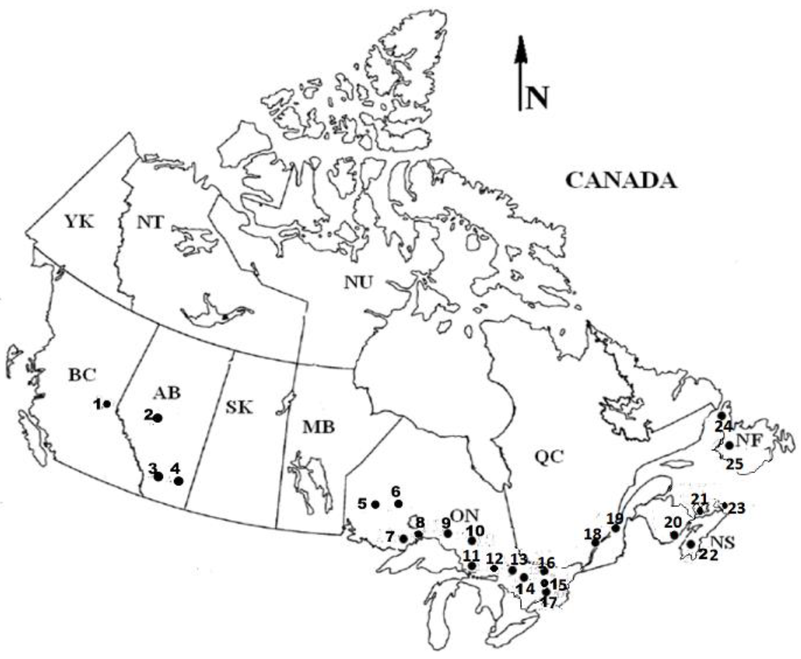
Figure 1.
Map of Canada showing the hydrometric gauging stations (source: Environment Canada).

It is imperative that in the DM-based procedure, the flow sequences must be stationary. Therefore, standardization of the annual, monthly and weekly sequences is achieved and the resultant sequences are known as SHI sequences, which turn out to be weakly stationary (i.e., second-order stationarity). At the annual time scale, the draft is set at the levels 1 µa, 0.9 µa, 0.8 µa, 0.75 µa, etc. The SHI sequences are truncated at these draft levels to carry out analyses in the DM-based procedure. For example, in the Bow River case at the annual time scale (Table 1: µa = 38.96 m3/s and cva = 0.13; the suffix “a” stands for annual) with the draft = 1 µa, the truncation (SHIx) level in the SHI sequence can be determined by the relationship, SHIx = (αµa − µa)/σa = (α − 1)/cva = (1 − 1)/0.134 = 0. At the draft of 0.75 µa (α = 0.75), the truncation level (SHIx) shall turn out to be (0.75−1)/0.134 = −1.87. Because of a single value of SHIx, the analysis is tractable at the annual scale for all the draft levels (i.e., 1µa, 0.90 µa, and 0.75 µa).
At the monthly scale with a draft level of 1 µa (=1 µo), the SHI sequences are truncated at SHIx = 0 to correspond to the variable monthly means. It should also be realized that µa (annual mean) = µo (overall monthly mean) and thus, these terms can be used interchangeably. The SHI sequence obtained has uniform µ = 0 and σ = 1 across the months. The sequence is construed as stationary and is tractable using the known methods of stochastic analysis. However, at 0.75 µo, there shall emerge 12 values of SHIx to truncate the SHI sequence. For example, in the Bow River case at the draft level of 0.75 µo, the 12 values of cv vary from 0.12 to 0.41 with the corresponding SHIx values ranging from −2.11 to −0.62 (Table 1). Thus, the SHI sequence needs to be truncated by variable SHIx values (or a curve rather than a horizontal line), which presents a complex scenario requiring some procedures such that known methods of statistical analysis for the estimation of drought magnitude can be applied. The above description can be extended to weekly flows and corresponding SHI sequences.
2.1. Strategies for Truncating the Non-Stationary (Monthly) Flow Sequences
At draft levels less than 1µo, such as 0.75µo, one way of conducting the DM-based analysis is through selecting varying values of “α” with respect to each month in order to render the SHIX = (α1 − 1)/cv1 = (α2 − 1)/cv2 = (α3 − 1)/cv3 = (α4 − 1)/cv4 --- = (α12 − 1)/cv12 = ‘SHIo’ (say). It is noted that cv1 is defined herein as the ratio of σ1 (standard deviation of month 1) to µ1 (mean of month 1), and likewise for the rest of the months. The value of ‘SHIo’ thus obtained is representative of the flat standardized value of 0.75µo of the monthly flow sequence with the overall µo = 38.96 m3/s and σo = 40.85 m3/s, and consequently cvo = 1.05 (italicized value in the last column (labelled as remarks) shown in Table 1) for the Bow River. There is a difference between the overall σo (=40.85 m3/s) and σav (=9.44 m3/s). The value σav (=9.44 m3/s) is the arithmetic average of 12 values of σ’s corresponding to their respective months. Hence, one value of ‘SHIo’ is obtained by the flat standardization of the 0.75 µo viz., ‘SHIo’ = (0.75 µo − µo)/σo = (0.75 − 1)/cvo = −0.24 with cvo = 1.05 (also indicated earlier). In the case of the monthly SHI sequences for the Bow River, at ‘SHIo’ = −0.24 the values of “α” (say: α1, α2, α3, … α12) are obtained as 0.97 (= –0.24 × cv1 + 1), 0.97, 0.97, 0.93, 0.90, 0.94, 0.94, 0.95, 0.95, 0.95, 0.96 and 0.96. These values of “α” (denoted as α’) are varying from 0.90 to 0.97 with a mean value of 0.95. In other words, at the draft of 0.75 µo, the monthly flows are being truncated at the aforesaid α’ levels of the respective monthly means, which still maintain a horizontal straight line across the months.
Other considerations for obtaining values of the ‘SHIo’ could be as follows: (1) the average of 12 monthly values of SHIx (denoted as SHIav), (2) the maximum of 12 SHIx values (denoted as SHIm), or (3) any other combination of these 12 values. Thus, the quantity “SHIav” is defined to be equal to “(α − 1) × µo/σav”, and likewise the quantity “SHIm” to be equal to “(α − 1) × µo/σmax” (where σmax is the maximum value among 12 monthly values of standard deviations). The above analogy can also be extended to the weekly flows, where there are 52 values of α’. The hypothesis proposed in the paper is that the ‘SHIx’ = ‘SHIo’ (a flat standardized value), and the use of SHIm or SHIav for truncating the SHI sequences provides a reasonable procedure to evaluate the drought magnitude as an estimator for the reservoir volume at the draft of 0.75 µo. The best estimate from the above combinations can be assessed by comparing the DM-based results with the SPA-based outputs.
2.2. Computation of Drought Magnitude (MT-o) by the DM-Based Counting Method
In the DM-based counting method, the SHI sequence is truncated at the level SHIx. The values of the SHI below the truncation level (SHIx level) are referred to as the drought (dubbed as ‘d’); whereas, the values of the SHI above the truncation level are referred to as the wet (dubbed as ‘w’). Initially, at each time scale, the value of SHIx is set = ‘SHIo’. In a historical record of N (=T) years, there could emerge several spells of drought (or dry) and wet conditions, only the length of the longest drought spell (denoted as LT-o) is counted. The absolute values of the drought intensities in the longest drought spell are added to represent the largest drought magnitude (MT-o). The largest deficit volume (DT-o) during a drought spell is computed as DT-o = σ × MT-o for the annual and DT-o = σav × MT-o for the monthly flow sequences. It should be noted that the subscript ‘o’ stands for the observed, that is, DT-o and MT-o, respectively, are the observed entities. Likewise, when these entities are estimated analytically, the subscript ‘e’ is used such as MT-e and DT-e. All the calculations are done in terms of MT-o (MT-e), or drought magnitude, which are converted to DT-o (DT-e), i.e., deficiency volume by the aforesaid linkage relationship.
2.3. Estimation of Drought Magnitude (MT-e) by the DM-Based Analytical Method
For a given return period (T), the longest drought period (LT), and the corresponding drought magnitude (MT), can be estimated using the drought magnitude-based analytical method for which the parameters are derived from the historical flow data (or regional patterns of these parameters). In the DM-based analytical method, the probabilistic relationship for MT can be obtained by applying the extreme number theorem [28] and utilizing the linkage relationship. The following applies: drought magnitude (M) = drought intensity (Id) × characteristic drought length (Lc). The drought intensity (Id) can be assumed to follow a truncated normal probability density function (pdf) and the drought magnitude (M) to obey the normal pdf because this quantity represents the summation of the drought intensity spikes. The mean and variance of “Id” are evaluated using the truncated normal pdf. The longest drought duration (LT) is estimated by the Markov chain (MC)-based relationship, which is shown as Equation (A9) in Appendix A. From the above linkage relationship, the terms MT and LT are related and thus, for design purposes over a time period (T), it is imperative to obtain the longest drought duration (LT) for the estimation of the term MT. On the monthly basis, the MC1 (Markov chain order 1) is a reasonable predictor (or estimator) of LT. In the MC1-based relationship, the four input parameters are conditional probabilities (qq, qp), plotting position factor (F), and return period (T) which is normally assumed to be equal to the sample size. The conditional probabilities qq (i.e., present period is drought given that the past period was also drought) and qp (i.e., present period is drought given that the past period was wet) are estimated based on the analytical relationship due to Cramer and Leadbetter [29]. In the present analysis, the relationship F = 1.33(1 + 0.25/T), developed for Canadian rivers by Adamowski [30], was used. The MC-based value of LT can be reduced to the characteristic drought length (Lc) by using a simple weighing parameter Φ (ranging from 0 to 1), which can also be obtained through an optimization procedure.
Based on the above notions for the estimation of MT, the following probability-based relationship can be deduced (see: Appendix A for detail).
Equation (1) is a discrete version of evaluating the mean from the first principles, and the following applies: [µ = E(x) = ∑x p(x), where x is a value of the random variable with the occurrence probability = p(x)]. The notation P (.) stands for the cumulative probability and p (.) stands for the simple probability. Since MT is a continuous random variable, and thus possesses a continuous pdf such that p (MT = Yj) can be evaluated as P (MT ≤ Y j+1)–P (MT ≤ Yj) with MT = Yj replaced by the mean value It is noted that the upper limit of summation (n1) will vary from the annual to monthly scales. For the annual scale, the maximum value of Y = 30 was found to be sufficient, whereas for the monthly scale, the maximum value of Y = 150 was found to be adequate. For integration purposes, the Y is discretized into small intervals with a step (∆) of 0.05, such that n1 becomes equal to 600 (=30/0.05) at the annual scale, and likewise equal to 3000 for the monthly scale. For purposes of numerical integration, thus, these Yj’s shall take on the values as 0, 0.05, 0.10, 0.15, etc., up to 150 at the monthly scale and up to 30 at the annual scale.
A simplified version for the estimation of E (MT) can be developed based only on the mean of the drought intensity as follows:
It should be borne in mind that Equation (1) involves implicitly both the mean and variance of drought intensity (Id) for the estimation of E (MT). Relevant detail on the derivation of Equations (1) and (2) is provided in Appendix A.
At the monthly and weekly scales, the SHI sequences of Canadian rivers have been reported by Sharma and Panu [23] to follow a gamma pdf vis-à-vis the normal pdf for the annual SHI sequences. In such a situation, firstly the gamma-distributed SHI value at the desired truncation level (denoted as SHIx) is transformed into an equivalent standard normal number z0 using the following Wilson–Hilferty transformation, as documented in Viessman and Lewis [31]:
A corresponding value of the drought probability (q) can be obtained from the following polynomial equation [32]:
where, B = q for z0 < 0; and q = (1 − B) for z0 ≥ 0 and the term |z0| represents the absolute value of z0. The error evaluated by this formula is less than 0.00025 and exactly the same value is obtained from a standard normal probability table for z0 = 0 (i.e., q = B = (1 − 0.5) = 0.5).
As an illustrative example, consider the Bow River, which obeys the gamma pdf with cvav = 0.24 at the monthly scale (Table 1) for a value of SHIx = −0.24. The corresponding z0 = −0.16 was obtained using the Wilson–Hilferty transformation given in Equation (3). Substituting z0 = −0.16 in Equation (4), the value of q would result to be 0.45. It is reported earlier in the text that monthly flow sequences in Canadian rivers tend to follow the gamma pdf, and for this reason, the gamma pdf has been used in this example.
In the DM-based procedure, DT-e (or DT-o) should correspond to VR obtained from the SPA, in turn, such an expectation forms the criterion for perfecting the DM-based estimates. Once the DM-based estimates for an appropriate LT and MT are evaluated (either by the counting or analytical methods), then these quantities are used for the estimation of reservoir volumes. Analytically derived E (MT) is denoted as MT-e and correspondingly, DT-e = σav × MT-e (subscript “e” stands for analytically estimated).
3. Data Set and Computations of Reservoir Volumes by the SPA and DM-Based Methods
Twenty-five rivers from Western to Atlantic Canada (Figure 1, Table 2) were involved in the analysis. The rivers encompassed drainage areas ranging from 46 to 74,600 km2 with the data bank spanning from 36 to 106 years. The monthly and annual flow data for these 25 rivers were extracted from the Canadian hydrological database [33]. The weekly flows were collated using the daily flow data for the above gauging stations. The values of the statistical parameters µ, σ, cv, and ρ for these rivers at annual, monthly and weekly scales were computed and are summarized in Table 2. Since cv = σ/µ, therefore instead of σ, the values of cv are summarized (Table 2) for the sake of brevity and ease of comprehension. In the case of the monthly and weekly flow sequences, there are 12 and 52 values of cv (or σ) that were used in respective standardization. The cvav was computed as the ratio of σav (arithmetic average of 12 monthly values) to µo (overall monthly mean or MAF, µa) and similar calculations also apply to the weekly scale. The first step in the analysis was to compute the statistics viz., µo and σo of the monthly sequences for the flat standardization of these sequences. Likewise, these statistics were computed for the weekly flow sequences. The flat standardized values of cv at monthly and weekly scales are denoted as cvo and cvow. The flat standardized values of ‘SHIo’ were computed at the 0.75µo level of cutoff using the overall µ (=µo) and σ (=σo or σow) of the non-stationary monthly and weekly flow sequences, and are shown in Table 3.
3.1. Inter-Comparison of Reservoir (VR) and Deficit (‘DT-o) Volumes for the Draft of 0.75 µo at Varying Time Scales
The analysis commenced with the computing of VR and ‘DT-o at the annual, monthly and weekly scales and the results for 25 rivers are summarized in Table 3. It is reiterated here that VR (m3, SPA) and ‘DT-o (m3, counted as the deficiency volume) are the entities that were computed from the non-standardized annual, monthly and weekly sequences for the draft equal to 0.75 MAF (=µa). A distinction is made between ‘DT-o and DT-o, in which both the entities stand for the deficit volume, but the former one is counted directly from the non-standardized flow data (without involving standard deviation) and the latter one is computed from the relationship DT-o = σ × MT-o involving the SHI sequences. At the annual scale, ‘DT-o = DT-o because of a single value of σ. On the monthly scale, a discrepancy may erupt between ‘DT-o and DT-o because of a selection of the representative value of σ among the 12 monthly σ’s. The best estimator for this purpose was found as σav, i.e., an arithmetic average of the 12 monthly σ values [24]. However, ‘DT-o is the true estimate of the deficiency volume and that is why it has been used for comparing with VR in the present analysis. The cutoff level is taken = (0.75 − 1) µa/σa for the annual, (0.75 − 1) µo/σo for the monthly and (0.75 − 1) µo/σow for the weekly flow sequences. Since the computational process for ‘DT-o does not require any standardization, there was no need to obtain the SHI sequences. The most striking observation (Table 3) is that at the monthly and weekly scales, the VR values are much larger than those at the annual scale. The VR values at the monthly scale were found to be almost 200% (average = 199% in Table 3) compared to the annual scale, but at the weekly scale the increase was found to be marginal (3.3%) concerning the monthly values.
At each time scale, the values of ‘DT-o were found to be less than VR. However, in general, a parallel trend in the values of ‘DT-o being similar to VR is apparent, although such values tend to increase from the annual to monthly scale. However, an increase in the ‘DT-o values at the weekly scale is not consistent because of random occurrences of a marginal decreases in values, which can be ascribed to sampling variations. At the annual scale, the VR and ‘DT-o values are almost equal, though at times they turned out to be zero, for example, 2 rivers (#23 North Margaree and #24 Upper Humber in Table 2). For these two rivers, there appears to be no need for storage at the draft of 0.75 µa based on the annual flow analysis. This finding seemingly is less convincing as there are long dry periods rendering the presence of low flows in these rivers, requiring compensating flow releases from storage. Therefore, the aforesaid analysis at the annual scale provides fewer functional estimates of the reservoir and the corresponding deficiency volumes at the draft level of 0.75 µa. However, more functional estimates are obtained by analyzing at the monthly and weekly scales. At these scales, to meet the draft of 0.75 µa, storage is required in the form of reservoirs across the above rivers, as evinced by significant storage values (Table 3). Another point to be noted is that the cutoff level ‘SHIo’ at the annual scale shows large variability (range −0.68 to −2.03) compared to the monthly and weekly scale, where variability is contained within a small range (from −0.17 to −0.34).
The aforesaid analysis thus points out that the monthly based VR values are drastically different from those obtained at the annual scale. The weekly based estimates are marginally higher than the monthly based, so monthly analysis seems to be adequate. Further, at the monthly and weekly scales, ‘SHIo’ is varying within a close range and thus, either of the time scales can be considered for further analysis, weighing the choice to the monthly scale because of its affable tractability in terms of statistical analysis. The monthly values are easy to procure and/or synthesize. The monthly SHI (standardized flow) sequences fit well within the MC1 dependence structure, which is better amenable for analysis using stochastic methods. Because of the above observations, the detailed analysis for computing VR, DT-o and DT-e has been done on the monthly flow and SHI sequences, and the methods of analysis are presented below.
3.2. Implementation of the DM-Based Counting and Estimation Methods
In the DM-based methods, the first step was to form the moving average (MA) smoothed sequences from the monthly SHI sequences. In the present paper, the SHI sequence by itself is taken as the MA1 (moving average 1) smoothing with µ = 0 and σ = 1. In the MA2 smoothing, 2 consecutive values of SHI were averaged out, and a running smooth sequence of MA2 was formed with µ = 0 and σ (designated as σm2), which turned out to be smaller (<1) than the case of MA1. Intuitively, a higher degree of smoothing leads to a higher dependence and that is why ρ (denoted as ρm2) for the MA2 case will be greater than that (ρm1) for the MA1 case. The MA2 sequence was again standardized using µ = 0 and a new value of σ (denoted as σm2) for further analysis.
In the counting process, the SHI sequence was truncated at the level of SHIx (i.e., SHIx = SHIo, SHIx = SHIm, and SHIx = SHIav) in both the cases of the MA1 and MA2 sequences. The values of the above three SHIx at the monthly scale are summarized in Table 4. There will be two values of MT-o based on the MA1 and MA2 sequences, which, in turn, will be converted into DT-o values by the relationship DT-o = σav × MT-o. It should be noted that the unit of DT-o is the same as that of σav as MT-o because being a standardized quantity is a dimensionless entity. At each smoothing, the multiplier will be σav with MT-o.
On the other hand, in the analytical procedure, the values of LT-e, MT-e and DT-e were evaluated by involving Equations (1) to (4), and other relevant equations (Appendix A), with the parameters (cvav, σav, ρm1 and ρm2) estimated from the observed flows and SHI sequences. A value of Φ in determining the characteristic length LC was needed, which required a calibration, though the initial values are available from the investigations of Sharma and Panu [26]. Such values have been further affirmed through an evaluation using the Nash–Sutcliffe efficiency (NSE) and the mean error (MER) criterion. To convert MT-e into DT-e, the original value of σav was used as a multiplier similar to the case of the counting method.
4. Results and Discussion
4.1. Comparison of VR’ and MT-o at Monthly Scale with SHIo as Cutoff: By Counting Method
It must be reiterated that the DM-based method is applied to the SHI sequences. For comparative analysis, VR, DT-o (by the counting method), and DT-e (by the analytical estimation) were made non-dimensional, and thus homogeneous, by dividing each of them by the same value of σav for their respective rivers. Thus, the terms VR, DT-o, and DT-e were transformed into VR’, MT-o, and MT-e for all the comparisons and are summarized in Table 4. For brevity, all the rivers are not listed in Table 4, rather included are two typical and representative rivers from each of the three regions. The selection criterion for choosing a river was the persistence characteristics represented by the lag-1 autocorrelation (ρm1). The first set of two rivers (#3 and #5) are located in the Prairies and Western Ontario with ρm1 ≥ 0.5; the second set of rivers (#8 and #11) are from Northern Ontario with 0.25 < ρm1 < 0.5; and the third set of rivers (#20 and #25) are from Atlantic Canada with a modest autocorrelation (i.e., ρm1 < 0.25). However, it should be noted that the performance statistics (NSE and MER) reported in Table 4 and all graphical displays are based on all the 25 rivers, and accordingly, the results are discussed. For comparative analysis of any pair on a 1:1 basis, the performance statistics (NSE and MER) were used. For an acceptable quality of parity in the entities in a pair, one should expect the value of NSE to be greater than 75% along with the value of MER to be within ±5% [23].
Based on the results of the analyses, it was found that MT-o in terms of the MA1 sequences underestimated VR’ (MER ≈ −14%) whereas, it was overestimated (≈15%) in the MA2 sequences with an NSE of less than 60% (Table 4, columns 4 and 5). These values, therefore, suggest that the counting-based procedure for evaluating DT-o to match VR can be interpreted as unsatisfactory. This discrepancy necessitated an alternative method to evolve estimates for deficiency volumes (DT) comparable to SPA-based (VR) values. Therefore, recourse was taken to an analytical method in which the probability-based relationships (Equations (1) and (2)) formed the basis for the evaluation of the needed entities.
4.2. Comparison of VR’ and MT-e (Equation (2)) at the Monthly Scale with SHIo as Cutoff
The simple procedure in the ambit of estimation methods is the use of Equation (2), in which MT-e = . Therefore, the MT-e values for the MA1 and MA2 smoothed sequences were computed by evaluating the terms µd and LT. The comparison of the MA1 sequences based on MT-e resulted in underestimation with MER (≈−32%) and an NSE of 43% (Table 4, columns 6). The MT-e estimates (Table 4, column 7) based on the MA2 sequences seemed better with MER ≈ 0, but the NSE was low (≈46%). Such values appear to be stoic and allude to the modest potential of the simple equation to provide acceptable estimates for the reservoir volumes. Similar behavior of Equation (2) at the draft of 0.95 to 1 MAF has been reported [25], where a substantial underestimation was observed. Because of the foregoing observations, it is imperative to extend to a step higher model (Equation (1)), which involves both the mean and variance of drought intensity for the estimation of MT-e.
4.3. Comparison of VR’ and MT-e (Equation (1)) at Monthly Scale with SHIo as Cutoff
In the analytical method using Equation (1), the crucial parameter is Φ because it controls the value of the characteristic drought length, Lc. The experience of authors on Canadian rivers suggests that two values of Φ, viz. 0 and 0.5, be considered for use in Equation (1). The values of MT-e were estimated based on the MA1 and MA2 smoothed sequences along with Φ = 0 and 0.5, and the results are summarized in Table 4.
The values of MT-e were computed by involving only MA1 sequences along with Φ = 0 and the results are presented in Table 4, column 8. It is apparent that the MT-e values in column 8 are generally larger than VR’ (column 3), thus indicating an overestimation. This fact is also reflected in MER ≈ 27%, though the value of NSE was reasonable (≈76%). Therefore, a value of Φ = 0.5 was attempted on the MA1 sequences, which resulted in the underestimation (MER ≈ −14%) and a low value of NSE ≈ 62% (Table 4, column 9). Since the results based on the MA1 sequences turned out to be less than encouraging, it was considered appropriate to estimate MT-e using the MA2 sequences with values of Φ = 0 and 0.5, and the results thus obtained are exhibited in columns 11 and 12 (Table 4). A striking feature on the MA2-based computations is the significant overestimation (MER ≈ 99% for Φ = 0; and MER ≈ 35% for Φ = 0.5).
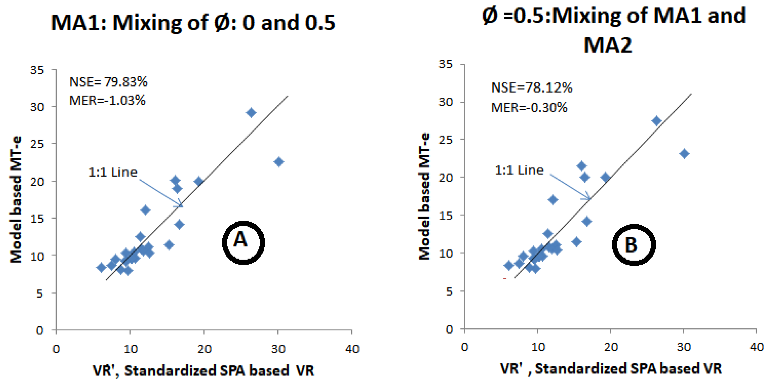
With the use of Φ = 0.5 on the MA1 sequences, major discrepancies were noted in the rivers lying in Prairies and Western Ontario (#1 to #6) in which ρm1 was ≥0.5, whereas the rivers from #6 to #25 tended to show reasonable correspondence. It can, thus, be conjectured that the same value of Φ is not applicable uniformly in all the rivers. Therefore, the following two groups of rivers were formed: group 1 was river #1 to #6 and group 2 was river #6 to #25. The discrepancy in group 1 was ameliorated with the use of Φ = 0, while retaining Φ = 0.5 for the rivers in group 2. Likewise with Φ = 0.5 on the MA2 sequences in the group 1 rivers, but Φ = 0.5 on the MA1 sequences in the group 2 rivers tended to improve the matching. This mooted the idea of mixing Φ’s (0 or 0.5) on the MA1 sequences (named as combination-A) or mixing the MA1 and MA2 sequences with Φ = 0.5 (named as combination-B). Based on the use of differential values of Φ on the MA1 sequences in combination-A, the resultant MT-e values are arranged in column 10 (Table 4). The combination-A-based values of MT-e compared satisfactorily with VR’ as shown in Figure 2A (MER ≈ −1% and NSE ≈ 80%). Likewise, in combination-B the MT-e values with differential MA (MA1 or MA2 sequences) with a uniform value of Φ = 0.5 are arranged in column 13 (Table 4). The combination-B resulted in NSE = 78% with negligible overestimation of 1.5% (Figure 2B).
Although, the estimated values of MT-e under both combinations (i.e., A and B) do not appear significantly different but one would be inclined to use combination-A with the use of differential values of Φ on the MA1 sequences for estimation purposes of MT-e. This is because working on the MA1 (which is the SHI itself) sequences is easier and convenient as the Φ values can be easily plugged in the desired equations. A worthy point to note is that the combination-B involves the MA2 sequences, thus warrants making another sequence (extra effort) based on the SHI sequences and also evolving a new set of parameters, viz. ρm2 (lag-1 autocorrelation of MA2 sequences) and σm2 (standard deviation of MA2 sequences), which is not devoid of uncertainty and errors.
4.4. Comparison of VR’ and MT-e (Equation (1)) at Monthly Scale with SHIm and SHIav as Cutoff
Although SHIo seemed reasonably satisfactory as a cutoff for the MA1 sequences, there is still a noticeable divergence in the higher range of values of these entities (Figure 2A,B) between VR’ and MT-e. Should this divergence be mitigated, the NSE would improve, alluding to a better fit. Since VR’ is already a fixed entity, the divergence can be reduced by improving the values of MT-e. Therefore, two versions of SHIx were contemplated, namely, SHIm and SHIav. SHIm is computed as = (0.75 − 1)/cvm and SHIav = (0.75 − 1)/cvav, where cvm = σmax/µo, cvav = σav/µo, and σmax is the maximum value among 12 monthly σ’s, whereas σav is the arithmetic average of these 12 monthly values. The new values of SHIx as SHIm and SHIav are shown in Table 4 (in the mid and lower portion of column 2) for the rivers under consideration. These cutoff levels were applied on the MA1 and MA2 sequences in the same manner as was conducted with cutoff = SHIo while using Φ = 0 and 0.5. The results based on the new values of SHIx (=SHIm) for MT-e are shown in Table 4 (columns 8 to 13). With the SHIm as the cutoff, the fit has improved yielding the NSE value ≈ 85% (combination-A, mixing of Φ values) and ≈ 86% (combination-B, mixing MA1 and MA2). The MER also remained within 3% suggesting an acceptable overestimation.
The new values of MT-e against VR’ are shown in Figure 3A,B, where the points fall closer to the 1:1 line vis- à-vis Figure 2A,B, where they lie farther from the 1:1 line. At a first glance, the plots further suggest that SHIm can be construed to be a better cutoff level compared to the SHIo, though only marginally. A further attempt was made to engage SHIav, and the new estimates of NSE and MER were evaluated (the lower portion in Table 4, columns 10 and 13). The response with SHIav as the cutoff was less than promising as MER indicated underestimation in the range of nearly 26% (combination-A) and 22% (combination-B). It can be perceived from Table 4 (column 2) that the values of SHIav appear significantly different from SHIo and SHIm, thus yielding low values of MT-e in comparison with VR’. Consequently, no further analysis was pursued using SHIav as a candidate choice. Prima-facie, SHIm appears to be a better cutoff followed by SHIo and further investigations were needed to discriminate between these two cutoffs to evolve the better one. The relative difference between VR and DT-e was considered a better measure for the discriminant analysis and was conducted as follows.
4.5. Relative Difference between Deficit Volume (DT-e) and Reservoir Volume (VR)
The performance statistics NSE and MER essentially help to discern the quality of a fit between MT-e and VR’ about the 1:1 line because both are respectively standardized values of DT-e and VR. Also, the large variations within DT-e and VR are not accurately accounted for by NSE and MER statistics. The relative difference in percent (designated as a relative error, RE), i.e., RE (=100 × (DT-e − VR)/VR) can be used as a robust measure to express the adequacy of the estimated values of DT-e as a competing estimate of VR. Preferably, RE should be close to zero for an ideal estimate of DT-e, and conversely, a higher value indicates a poor estimation. Thus, based on the DT-e and VR values of 25 rivers, the RE values were evaluated for the two cutoff conditions, viz. SHIx = SHIo and SHIx = SHIm involving both combination-A and combination-B. The mean (designated as µre) and standard deviation (designated as σre) of these 25 RE values were computed and are presented in Table 5. The cutoff equal to SHIo with combination-A yielded the least µre = 0.77% (σre ≈ 17%) followed by µre = 1.52% (σre ≈ 18%) with combination-B. The cutoff equal to SHIm outputted µre close to 4% (σre ≈ 17%) in both combination-A and combination-B. Given these statistics, one can interpret that SHIo is a better cutoff than SHIm, which contradicts the earlier finding (based on NSE and MER) that had placed SHIm ahead of SHIo.
It is worthy to note that µre and σre (not tabulated in Table 5) were also evaluated for the cutoff equal to SHIav, which resulted in µre ≈ −24% (σre ≈ 14%) for combination-A and likewise, µre ≈ −22% (σre ≈ 14%) for combination-B. These values (specifically the µre values), being far from the desired value of 0, further support the earlier argument of rejecting SHIav as a viable and competing cutoff level.
At this point, there is a need to discriminate between SHIo and SHIm, and to suggest a consistent cutoff level for estimating the deficit volumes (=reservoir volumes), as the statistics MER and RE have not rendered unanimous results. This anomaly was solved by enlarging the sample size from 25 (each river is a sample) to 37. The rivers with a long record (#3, #5, #19, #20, #22 and #23 in Table 2) were split into two samples, each of nearly equal size, and VR and DT-e values were computed for 37 (25 + 12) samples. Based on the 37 samples, the MER (using MT-e and VR’) and RE (using DT-e and VR) were evaluated and the results are shown in Table 5 at the cutoff levels of SHIo and SHIm for combination-A and combination-B. For the cutoff level (SHIm), the new µre values were found to range between 3 to 4% (σre > 18%) but the NSE values dropped significantly from 85% to 73%. This is undesirable behavior, and thus the reliability of the cutoff (SHIm) lands in a doubtful regime. In contrast, the behavior of the cutoff (SHIo) is more consistent because the NSE values remained closer to each other in both samples of the original 25 flow datasets and the latter 37 flow datasets. Further, the µre values were found to be closer to 0 (ranging from 0.77 to 3.91%). Based on these numbers, it can be easily conjectured that the cutoff (SHIo) is better compared to the cutoff (SHIm). Needless to mention, it is easy to derive SHIo values by computing µo and σo (or cvo) from the non-stationary monthly flow sequences. Likewise, the ρm1 and σav can also be rapidly computed from the monthly flow and SHI sequences.
To objectively illustrate the DM-based methodology, an example is presented using the monthly data of the following two rivers: the English River (#5 in Table 2, with a high value of ρm1 = 0.76) and the Neebing River (#7 in Table 2, with a modest value of ρm1 = 0.43). The relevant specificities and computations for these rivers are as follows.
English River: T = 92 years (1164 months), µo = 58.61, cvo = 0.74, cvav = 0.51, ρm1 = 0.76, and ρm2 = 0.88. Since ρm1 = 0.76 (>0.50), so Φ = 0. Plugging the above parameters in the relevant equations, DT-e was computed as 2.26 × 10⁹ m3. The SPA-based value of VR was computed as 2.04 × 10⁹ m3. The relative difference is therefore +11% (indicating an overestimation compared to the SPA-based value), which is reasonably acceptable. The above estimate can be attached to a return period of 100 years (sample size 92 years ≈ 100 years). The other merit of the DM-based method is the estimation of DT-e with any other return period, say 50 years (600 months). Plugging T = 600 into the relevant equations, DT-e = 1.92 × 10⁹ m3, which is less than the 100-year value (=2.04 × 10⁹ m3).
Neebing River: T = 66 years (792 months), µo = 1.62 m3/s, cvo = 1.48, cvav = 0.81, ρm1 = 0.43, and ρm2 = 0.73. Since ρm1 = 0.43 (<0.50), so Φ = 0.5. Plugging the above parametric values into the relevant equations, DT-e was computed as 4.83 × 10⁷ m3. The SPA-based value of VR was computed as 5.69 × 10⁷ m3. The relative difference is therefore about −15% (an underestimation compared to the SPA-based value), which is again within an acceptable range of error. The above estimate can be attached to a return period of 66 years. The DT-e value with the return of T = 50 years or 600 months was computed as 4.58 × 10⁷ m3 and also for T = 100 years or 1200 months as 5.20 × 10⁷ m3. These DT-e estimates are closer to the SPA estimate of 5.69 × 10⁷ m3, with a slight underestimation. For design application, the VR can be taken as the average of 5.69 × 10⁷ and 4.83 × 107 = 5.26 × 10⁷ m3 for T = 66 years.
In a nutshell, the proposed analytical method yields satisfactory estimates of DT-e, which are comparable to the SPA-based estimates of reservoir volume, with a margin of error of ±18%. The combination with the length scaling parameter Φ = 0 and Φ = 0.5, respectively, for the rivers with high persistence and low persistence on the SHI (MA1) sequences proved adequate for estimation purposes.
Although in this analysis, the comparison has been made between SPA- and DM-based methods using the Canadian river flow data, it was considered appropriate to test the efficacy of the DM method using the data of the Mitta Mitta River (Australia) reported by McMahon and Mein (1978), and compare the estimates of the reservoir volumes by various other methods as shown in Table 6 (draft level of 0.75µ at the monthly scale). The estimate of the reservoir volume based on the DM method is also listed in the last row of this table.
It is evident from the above table that the estimate of reservoir volume by the DM (#9) lies between the SPA (#3), Gould Gamma (#6) and Behavioral analysis (#8). It has been reported (McMahon and Mein, 1978) that the Gould Gamma and Behavior analysis methods yield better results in terms of the least bias and standard error. In view of the foregoing observation, the DM-based estimate is relatively closer (i.e., within +14% error) to the above two estimates. While comparing with the SPA-based estimate, the DM-based estimate is slightly less (i.e., within −10.6%). Succinctly, the DM-based method offers an approach for the design of reservoir capacity, which opens a platform for comparison with techniques such as Extended deficiency analysis, Behavioral analysis, Hardison generalized method, Phien method, Vogel and Stedinger method, Gould’s probability method, etc., which have been discussed by McMahon et al. (2007). Such investigations of the aforesaid methods on Canadian rivers are underway by the authors under a separate study.
5. Conclusions
The DM-based methodology for reservoir sizing has been developed and applied at a 0.75 mean annual flow (MAF) level of the draft at the monthly scale in 25 rivers across Canada. The analysis, involving the annual, monthly and weekly flows at the aforesaid draft level, suggested that the monthly scale is the most optimal for the estimation of reservoir volumes at the draft of 0.75 MAF. The annual time scale was found inadequate. The weekly scale was adequate but only offered marginal benefits over the monthly based estimates of reservoir volumes.
In the DM-based methodology, the monthly standardized hydrological index (SHI) sequences were used to evolve the values of standardized drought magnitudes, MT-e, which were compared with the SPA-based standardized reservoir volumes, VR’. The DM-based analysis involved the MA1 (moving average 1) and MA2 sequences, which were formed from the SHI sequences. The SHI sequences themselves are denoted as MA1, while the averaged consecutive two SHI values formed the MA2 sequences. The cutoff level for truncating the MA1 and MA2 sequences was determined as SHIo = (0.75 − 1) µo/σo, where µo and σo are the overall mean and standard deviation of monthly flow sequences. Another competitive cutoff level was found as SHIm = (0.75 − 1) µo/σmax, in which σmax is the maximum value of standard deviation among 12 monthly values. In the DM-based methodology, one crucial parameter is the characteristic drought length, which is controlled (or optimized) through the length scaling parameter Φ. At the monthly scale, the value of Φ = 0 was found adequate for rivers with a lag-1 autocorrelation (ρm1) ≥ 0.5, and the Φ = 0.5 for rivers with ρm1 < 0.5. Two combinations of MA sequences were attempted to estimate MT-e, as follows: in combination-A, differential values of Φ (Φ = 0 for rivers with ρm1 > 0.5 and Φ = 0.5 for rivers with ρm1 < 0.5) were applied on the MA1 sequences; and in combination-B, a single value of Φ = 0.5 was applied on the differential MA sequences, i.e., MA1 sequences of rivers with ρm1 < 0.5 and MA2 sequences of rivers with ρm1 ≥ 0.5. Combination-A emerged to be better in terms of ease and convenience of computations while yielding MT-e values that are compatible with VR’. The DM-based estimates of deficit volumes (DT-e) were found to be closer to the SPA-based reservoir volumes (VR) within an error margin of ±18%. An important feature of the DM-based method is its ability to explicitly involve the return period in the estimation process, unlike the SPA, which yields estimates of reservoir volumes that are devoid of return periods.
Author Contributions
T.C.S. and U.S.P. collaboratively accomplished various tasks related to this manuscript, draft preparation and finalization of the manuscript for journal publication such as conceptualization and development of the methodology, data collection and data analysis. All authors have read and agreed to the published version of the manuscript.
Funding
This research was partially funded by the Natural Sciences and Engineering Research Council of Canada.
Institutional Review Board Statement
Not applicable.
Informed Consent Statement
Not applicable.
Data Availability Statement
Not applicable.
Acknowledgments
The partial financial support of the Natural Sciences and Engineering Research Council of Canada for this paper is gratefully acknowledged.
Conflicts of Interest
The authors declare no conflict of interest.
Appendix A
The following probability-based relationship from the first principles can be used to estimate the expected value of the largest drought-magnitude, E (MT):
The notation P (.) stands for the cumulative probability and p (.) stands for the simple probability. Since MT is a continuous random variable, therefore MT has a continuous pdf so p (MT = Yj) can be evaluated as P (MT ≤ Y j+1)–P (MT ≤ Yj) with MT = Yj replaced by the mean value Equation (A1) can therefore be expressed as the following:
The upper limit of integration, ∞ in Equation (A1), is replaced by some finite number n1. The general equation for evaluating P (MT ≤ Yj) based on the extreme number theorem [13] can be expressed as the following:
In which M takes on non-integer values represented by Yj. Since Y’s (such as Y1, Y2, Y3, Y4, etc.) correspond to values of M, thus the largest of them will correspond to MT. It is to be noted that M is the sum of several drought-deficit spikes encountered in a drought spell. Each spike has a negative sign because they are derived by truncating SHI sequences and they lay on the downside (negative side) of the cutoff level. The deficit spikes can be construed to obey a truncated normal distribution because a normal pdf encompasses values of a random variable from −∞ to +∞. Thus, the standard normal pdf is truncated at various levels of z0 (standard normal number) corresponding to counterpart values of the probability q. For example, a standard normal pdf can be truncated at z0 = −0.52 with the corresponding probability of 0.3, which can be obtained from the standard normal probability table or a polynomial equation documented in Chow et al. [32] and reiterated in the main text as Equation (4).
The truncated normal pdf version will have a mean and variance, respectively, different from 0 and 1. Applying the basic axioms for the evaluation of moments, expressions for the mean (denoted by μd) and variance (denoted by ) of the truncated normal pdf version can be deduced [15,16] as follows.
Because drought episodes lay below the desired truncation level, an absolute value of the term μd is an estimator of the mean value of drought intensity (Id), as it represents the mean of the several deficit spikes. Likewise, the term is an estimator of the variance of drought intensity, whose value is unaffected by the sign. For example, at the cutoff level of z0 = −0.52, q = 0.3; and the substitution of these values in Equations (A4) and (A5) yields μd equal to −0.64 and equal to 0.25. As explained earlier, the absolute value of μd will be taken as the mean value of the drought intensity (Id), i.e., = 0.64. Likewise, at the cutoff level, z0 = −0.10, q = 0.16; μd and will work out as −0.51 and 0.23.
Given the central limit theorem and since M is the sum of the deficit spikes, its probability structure can be approximated by a normal pdf with mean μM and variance [23]. Such a consideration reduces the expression for the term P (M ≤ Yj) in Equation (A3) as follows:
It was noted that the parameters μM and are related to the extreme drought length LT, and the mean drought length LM [24]. Such a representative drought length is named herein as a characteristic drought length LC, which can be expressed as follows:
LC = Φ LM + (1 − Φ) LT.
The parameter Φ can be designated as a weighing parameter as it weighs the mean drought length LM and the longest drought length LT. The value of Φ varies from 0 to 1 and is determined through optimization or a trial and error procedure. For first-order dependence or a Markov Chain order 1 (MC1) situation, the mean length LM can be expressed as follows [13]:
The expression for the expected value of LT in the MC1 situation in drought periods can be obtained as follows [24]:
where F is the factor to account for the plotting position in the empirical estimation of the exceedance probability. That is, in the Hazen plotting position formula, the exceedance probability = 0.5/T (T = sample size), so the return period is equal to T/0.5 = 2T or F = 2. Likewise, in the Weibull plotting position formula F = 1. In this analysis, the plotting position formula [30] as developed for Canadian rivers has been used. The formula evaluates the exceedance probability = 0.75/(T + 0.25), so F = 1.33 (1 + 0.25/T) ≈ 1.33 as T is generally large. The term qq stands for the conditional probability of the present period being drought given the previous period was also a drought, and likewise, qp stands for the present period being drought given the previous period was wet.
The conditional probabilities qq and qp can be computed from the following relationship due to Cramer and Leadbetter (29):
where is a dummy variable of integration while other terms are as defined earlier. The integral in Equation (A10) can be evaluated by a numerical procedure, and the values of qq for a given ρ and z0 can be computed. For the monthly SHI sequences ρ = ρm1. Equation (A10) can also be used to estimate pp (probability present time being wet given the past period was also wet) by replacing qq by pp and q by p (=1 − q). Therefore, an estimate of qp can be found as qp (=1 − pp), which can be used in Equation (A9) for the estimation of the longest drought lengths LT, involving the MC1 situation. Note for the MC0 situation, such as for the annual SHI sequences, qq = qp = q.
Once a proper value of LC has been determined, Equation (A6) is integrated numerically to evaluate P (M ≤ Yj) and then the value of the integrand is inserted in Equation (A3) to yield an estimate of P (MT ≤ Yj). Letting these values of Yj as Y0 (j = 0) = 0, Y1 (j = 1) = 0.05, Y2 (j = 2) = 0.10, Y3 (j = 3) = 0.15, Yn1 = 150 (for the monthly scale) with an increment, ∆ = 0.05, E (MT) can be computed using Equation (A3).
A particular version for the estimation of E (MT) can be developed based on the mean of the drought intensity, involving Equations (A4) and (A9) as follows:
Note, Equation (A2) involves both the mean and variance of drought intensity (Id) for the estimation of E (MT), and therefore is more comprehensive.
References
- Thomas, H.A.; Burden, R.P. Operation Research in Water Quality Management; Division of Engineering and Applied Physics, Harvard University: Cambridge, MA, USA, 1963. [Google Scholar]
- McMahon, T.A.; Mein, R.G. Reservoir Capacity and Yield; Development in Water Science #9, Elsevier: Amsterdam, The Netherlands, 1978; p. 78. [Google Scholar]
- Loucks, D.P.; Stedinger, J.R.; Haith, D.A. Water Resources Systems Planning and Analysis; Prentice-Hall: Englewood Cliffs, NJ, USA, 1981. [Google Scholar]
- McMahon, T.A.; Mein, R.G. River and Reservoir Yield; Water Resources Publications: Littleton, CO, USA, 1986. [Google Scholar]
- Linsley, R.K.; Franzini, J.B.; Freyburg, D.L.; Tchobanoglous, G. Water Resources Engineering, 4th ed.; Irwin McGraw-Hill: New York, NY, USA, 1992; p. 192. [Google Scholar]
- McMahon, T.A.; Adeloye, A.J. Water Resources Yield; Water Resources Publications: Littleton, CO, USA, 2005. [Google Scholar]
- Parks, Y.P.; Gustard, A. A reservoir storage yield analysis for arid and semiarid climate. IAHS Optim. Alloc. Water Resour. 1982, 135, 49–57. [Google Scholar]
- Lele, S.M. Improved algorithms for reservoir capacity calculation incorporating storage-dependent and reliability norms. Water Resour. Res. 1987, 23, 1819–1823. [Google Scholar] [CrossRef] [Green Version]
- Phien, H.N. Reservoir storage capacity with gamma inflows. J. Hydrol. 1993, 146, 383–389. [Google Scholar] [CrossRef]
- Adeloye, A.J.; Lallemand, F.; McMahon, T.A. Regression models for within-year capacity adjustment in reservoir planning. Hydrol. Sci. J. 2003, 48, 539–552. [Google Scholar] [CrossRef]
- Yevjevich, V. Stochastic Processes in Hydrology; Water Resources Publications: Littleton, CO, USA, 1972; pp. 179–211. [Google Scholar]
- Yevjevich, V. Methods for determining statistical properties of droughts. In Coping with Droughts; Yevjevich, V., da Cunha, L., Vlachos, E., Eds.; Water Resources Publications: Littleton, CO, USA, 1983; pp. 22–43. [Google Scholar]
- Sen, Z. Statistical analysis of hydrological critical droughts. ASCE J. Hydraul. Eng. 1980, 106, 99–115. [Google Scholar]
- Sen, Z. Applied Drought Modelling, Prediction and Mitigation; Elsevier Inc.: Amsterdam, The Netherlands, 2015. [Google Scholar]
- Guven, O. A simplified semi-empirical approach to probabilities of extreme hydrological droughts. Water Resour. Res. 1983, 19, 441–453. [Google Scholar] [CrossRef]
- Sharma, T.C. Estimation of drought severity on independent and dependent hydrologic series. Water Resour. Manag. 1997, 11, 35–49. [Google Scholar] [CrossRef]
- Tallaksen, L.M.; Madsen, H.; Clausen, B. On the definition and modeling of streamflow drought duration and deficit volume. Hydrol. Sci. J. 1997, 42, 15–33. [Google Scholar] [CrossRef]
- Salas, J.; Fu, C.; Cancelliere, A.; Dustin, D.; Bode, D.; Pineda, A.; Vincent, E. Characterizing the severity and risk of droughts of the Poudre River, Colorado. ASCE J. Water Resour. Plan. Manag. 2005, 131, 383–393. [Google Scholar] [CrossRef]
- Vicente-Serrano, S.M. Differences in spatial patterns of drought on different time scales: An analysis of the Iberian Peninsula. Water Resour. Manag. 2006, 20, 37–60. [Google Scholar] [CrossRef]
- Fleig, A.K.; Tallaksen, L.M.; Hisdal, H.; Demuth, S. A global evaluation of streamflow drought characteristics. Hydrol. Earth Syst. Sci. 2006, 10, 535–552. [Google Scholar] [CrossRef] [Green Version]
- Nalbantis, I.; Tsakiris, G. Assessment of hydrological drought revisited. Water Resour. Manag. 2009, 23, 881–897. [Google Scholar] [CrossRef]
- Lopez-Moreno, J.I.; Vicente-Serrano, S.M.; Beguria, S.; Garcia-Ruiz, J.M.; Portela, M.M.; Almeida, A.B. Dam effect on drought magnitude and duration in a transboundary basin: The lower River Tagus, Spain and Portugal. Water Resour. Res. 2009, 45, W02405. [Google Scholar] [CrossRef] [Green Version]
- Sharma, T.C.; Panu, U.S. Analytical procedures for weekly hydrological droughts: A case of Canadian rivers. Hydrol. Sci. J. 2010, 55, 79–92. [Google Scholar] [CrossRef]
- Sharma, T.C.; Panu, U.S. A simplified model for predicting drought magnitudes: A case of streamflow droughts in Canadian prairies. Water Resour. Manag. 2014, 28, 1597–1611. [Google Scholar] [CrossRef]
- Akyuz, D.E.; Bayazit, M.; Onoz, B. Markov chain models for hydrological drought characteristics. J. Hydrometeorol. 2012, 13, 298–309. [Google Scholar] [CrossRef]
- Sharma, T.C.; Panu, U.S. A drought magnitude-based method for reservoir sizing: A case of annual and monthly flows from Canadian rivers. J. Hydrol. Reg. Stud. 2021. in print. [Google Scholar]
- McMahon, T.A.; Pegram, G.G.S.; Vogel, R.M.; Peel, M.C. Revisiting reservoir storage–yield relationships using a global streamflow database. Adv. Water Resour. 2007, 30, 1858–1872. [Google Scholar] [CrossRef]
- Todorovic, P.; Woolhiser, D.A. A stochastic model of n day precipitation. J. Appl. Meteorol. 1975, 14, 125–127. [Google Scholar] [CrossRef] [Green Version]
- Cramer, H.; Leadbetter, M.R. Stationary and Related Stochastic Processes; John Wiley and Sons Inc.: New York, NY, USA, 1967. [Google Scholar]
- Adamowski, K. Plotting formula for flood frequency. Water Resour. Assoc. 1981, 17, 197–202. [Google Scholar] [CrossRef]
- Viessman, W.; Lewis, G.L. Introduction to Hydrology., 5th ed.; Prentice-Hall: Englewood Cliffs, NJ, USA, 2003; p. 59. [Google Scholar]
- Chow, V.T.; Maidment, D.R.; Mays, L.W. Applied Hydrology; McGraw-Hill: New York, NY, USA, 1988; p. 367. [Google Scholar]
- Environment Canada. HYDAT CD-ROM Version 96-1.04 and HYDAT CD-ROM User’s Manual. In Surface Water and Sediment Data Water Survey of Canada; Government of Canada: Ottawa, ON, Canada, 2018. [Google Scholar]
- Kotz, S.; Neumann, J. On the distribution of precipitation amounts for periods of increasing length. J. Geophys. Res. 1963, 68, 3635–3640. [Google Scholar] [CrossRef]
Figure 2.
Comparison of MT-e to SPA-based standardized reservoir volume with cutoff = SHIo: (A,B) respectively, represent Combination-A and Combination-B.
Figure 2.
Comparison of MT-e to SPA-based standardized reservoir volume with cutoff = SHIo: (A,B) respectively, represent Combination-A and Combination-B.

Figure 3.
Comparison of MT-e with SPA-based standardized reservoir volume with cutoff = SHIm: (A,B) respectively, represent Combination-A and Combination-B.
Figure 3.
Comparison of MT-e with SPA-based standardized reservoir volume with cutoff = SHIm: (A,B) respectively, represent Combination-A and Combination-B.

Table 1.
Summary of statistical parameters of annual and monthly flow sequences of the Bow River.
| Parameter | Months | Remarks | |||||||||||
|---|---|---|---|---|---|---|---|---|---|---|---|---|---|
| 1 | 2 | 3 | 4 | 5 | 6 | 7 | 8 | 9 | 10 | 11 | 12 | ||
| µ | 9.05 | 8.21 | 7.77 | 10.54 | 50.10 | 124.68 | 104.74 | 64.69 | 38.83 | 23.82 | 14.52 | 10.59 | Overall µ = µo = 38.96 † |
| σ | 1.22 | 1.15 | 0.92 | 3.15 | 20.35 | 30.71 | 26.28 | 13.15 | 7.44 | 4.72 | 2.61 | 1.55 | σav = 9.44, σo = 40.85 † σmax = 30.71 |
| cv | 0.14 | 0.14 | 0.12 | 0.30 | 0.41 | 0.25 | 0.25 | 0.20 | 0.19 | 0.20 | 0.18 | 0.15 | cvo = 1.05 |
| SHIx | −1.85 | −1.78 | −2.11 | −0.84 | −0.62 | −1.11 | 1.00 | −1.23 | −1.30 | −1.26 | −1.39 | −1.39 | |
| α’ | 0.97 | 0.97 | 0.97 | 0.93 | 0.90 | 0.94 | 0.94 | 0.95 | 0.95 | 0.95 | 0.96 | 0.97 | Mean of α’ = 0.95 |
Notation (†) stands for the values based on the nonstationary monthly flows. Annual statistics: µa = 38.96 m3/s; σa = 5.22 m3/s; cva = 0.134; ‘SHIo’ = −1.87 at 0.75µa, i.e., α = 0.75. At the monthly scale µo = 38.96 m3/s; σav = 9.44; SHIav = (0.75 − 1) × 38.96/9.44 = −1.03; and likewise, SHIm = (0.75 − 1) × 38.96/30.71 = −0.32. These numbers in bold and italic have been referred in the text.
Table 3.
Comparison of VR and DT-o at the draft level of 0.75µo: annual, monthly and weekly scales.
| River No. | Time Scale of the Analysis | Increase in VR (%) | ||||||||||
|---|---|---|---|---|---|---|---|---|---|---|---|---|
| Annual | Monthly | Weekly | ||||||||||
| SHIo | VR (m3) | ‘DT-o(m3) | SHIo | VR(m3) | ‘DT-o(m3) | SHIo | VR (m3) | ‘DT-o(m3) | ||||
| 1 | 2 | 3 | 4 | 5 | 6 | 7 | 8 | 9 | 10 | Month (%) | Week (%) | |
| 1. | −1.87 | 1.33 × 10⁹ | 1.33 × 10⁹ | −0.30 | 7.21 × 10⁹ | 7.21 × 10⁹ | −0.28 | 7.75 × 10⁹ | 7.34 × 10⁹ | 483 * | 7.5 ** | |
| 2. | −1.10 | 2.59 × 10⁹ | 2.59 × 10⁹ | −0.28 | 6.15 × 10⁹ | 4.17 × 10⁹ | −0.26 | 6.27 × 10⁹ | 4.41 × 10⁹ | 137 | 1.9 | |
| 3. | −1.87 | 4.18 × 10⁷ | 4.18 × 10⁷ | −0.24 | 4.01 × 10⁸ | 3.99 × 10⁸ | −0.23 | 4.25 × 10⁸ | 4.25 × 10⁸ | 854 | 6.0 | |
| 4. | −0.70 | 5.89 × 10⁹ | 4.06 × 10⁹ | −0.24 | 6.75 × 10⁹ | 4.45 × 10⁹ | −0.22 | 6.88 × 10⁹ | 2.48 × 10⁹ | 15 | 1.9 | |
| 5. | −0.77 | 1.54 × 10⁹ | 1.54 × 10⁹ | −0.34 | 2.04 × 10⁹ | 1.36 × 10⁹ | −0.32 | 2.07 × 10⁹ | 1.39 × 10⁹ | 33 | 1.5 | |
| 6. | −0.79 | 1.25 × 10⁹ | 1.25 × 10⁹ | −0.26 | 1.61 × 10⁹ | 0.71 × 10⁹ | −0.24 | 1.68 × 10⁹ | 0.73 × 10⁹ | 29 | 4.3 | |
| 7. | −0.68 | 3.61 × 10⁷ | 3.61 × 10⁷ | −0.17 | 5.69 × 10⁷ | 3.57 × 10⁷ | −0.13 | 5.81 × 10⁷ | 3.70 × 10⁷ | 58 | 2.1 | |
| 8. | −1.05 | 5.39 × 10⁸ | 5.39 × 10⁸ | −0.25 | 8.39 × 10⁸ | 7.38 × 10⁸ | −0.20 | 8.71 × 10⁸ | 7.60 × 10⁸ | 56 | 3.8 | |
| 9. | −1.00 | 2.23 × 10⁸ | 2.23 × 10⁸ | −0.21 | 4.63 × 10⁸ | 3.65 × 10⁸ | −0.17 | 4.92 × 10⁸ | 3.70 × 10⁸ | 107 | 6.3 | |
| 10. | −1.14 | 2.44 × 10⁸ | 2.44 × 10⁸ | −0.25 | 3.44 × 10⁸ | 3.40 × 10⁸ | −0.19 | 3.65 × 10⁸ | 3.40 × 10⁸ | 41 | 6.1 | |
| 11. | −1.25 | 0.74 × 10⁸ | 0.74 × 10⁸ | −0.24 | 3.37 × 10⁸ | 2.92 × 10⁸ | −0.21 | 3.44 × 10⁹ | 3.04 × 10⁹ | 355 | 2.1 | |
| 12. | −1.41 | 1.22 × 10⁸ | 1.22 × 10⁸ | −0.24 | 4.78 × 10⁸ | 3.75 × 10⁸ | −0.20 | 4.95 × 10⁸ | 4.95 × 10⁸ | 292 | 3.6 | |
| 13. | −1.17 | 1.31 × 10⁸ | 1.31 × 10⁸ | −0.24 | 2.61 × 10⁸ | 2.61 × 10⁸ | −0.19 | 2.70 × 10⁸ | 2.70 × 10⁸ | 161 | 3.5 | |
| 14. | −1.07 | 2.96 × 10⁷ | 2.96 × 10⁷ | −0.21 | 6.57 × 10⁷ | 3.53 × 10⁷ | −0.17 | 6.70 × 10⁷ | 4.31 × 10⁷ | 122 | 2.1 | |
| 15. | −1.21 | 1.09 × 10⁹ | 1.09 × 10⁹ | −0.24 | 1.72 × 10⁹ | 1.17 × 10⁹ | −0.23 | 1.79 × 10⁹ | 0.88 × 10⁹ | 58 | 4.1 | |
| 16. | −1.10 | 0.58 × 10⁷ | 0.58 × 10⁷ | −0.26 | 2.45 × 10⁷ | 2.21 × 10⁷ | −0.19 | 2.51 × 10⁷ | 2.01 × 10⁷ | 287 | 2.5 | |
| 17. | −1.06 | 1.37 × 10⁷ | 1.37 × 10⁷ | −0.27 | 3.76 × 10⁷ | 3.31 × 10⁷ | −0.23 | 3.80 × 10⁷ | 3.55 × 10⁷ | 174 | 1.1 | |
| 18. | −1.22 | 0.80 × 10⁸ | 0.80 × 10⁸ | −0.23 | 3.95 × 10⁸ | 3.95 × 10⁸ | −0.26 | 4.10 × 10⁸ | 3.01 × 10⁸ | 393 | 1.0 | |
| 19. | −0.98 | 1.17 × 10⁸ | 1.17 × 10⁸ | −0.21 | 2.42 × 10⁸ | 1.90 × 10⁸ | −0.24 | 2.41 × 10⁸ | 1.88 × 10⁸ | 107 | 0.0 | |
| 20. | −1.12 | 0.58 × 10⁸ | 0.58 × 10⁸ | −0.31 | 1.16 × 10⁸ | 0.77 × 10⁸ | −0.23 | 1.21 × 10⁸ | 0.79 × 10⁸ | 100 | 4.3 | |
| 21. | −1.20 | 0.75 × 10⁷ | 0.75 × 10⁷ | −0.24 | 1.38 × 10⁷ | 1.15 × 10⁷ | −0.19 | 1.44 × 10⁷ | 1.21 × 10⁷ | 84 | 4.3 | |
| 22. | −1.34 | 1.92 × 10⁷ | 1.92 × 10⁷ | −0.31 | 3.52 × 10⁷ | 3.09 × 10⁷ | −0.23 | 3.66 × 10⁷ | 3.38 × 10⁷ | 83 | 4.0 | |
| 23. | −1.74 | 0 storage | 0 volume | −0.33 | 1.28 × 10⁸ | 1.28 × 10⁸ | −0.26 | 1.33 × 10⁸ | 1.05 × 10⁸ | -- | 3.9 | |
| 24. | −2.03 | 0 storage | 0 volume | −0.29 | 8.74 × 10⁸ | 8.74 × 10⁸ | −0.23 | 9.28 × 10⁸ | 5.38 × 10⁸ | -- | 6.2 | |
| 25. | −1.70 | 0.38 × 10⁸ | 3.80 × 10⁷ | −0.29 | 2.49 × 10⁸ | 2.49 × 10⁸ | −0.23 | 2.56 × 10⁸ | 2.09 × 10⁸ | 555 | 2.8 | |
| Mean | 199% | 3.3% | ||||||||||
Asterisk (*) denotes the percentage increase in monthly value compared to the annual value. Asterisk (**) denotes the percentage increase in the weekly value of VR compared to the monthly value, and -- means no values were evaluated for the VR and DT-o because both were zero at the annual scale. These Bold numbers in the coulumns 3, 6, and 9 are SPA based numbers for comaparative purposes.
Table 4.
Comparison of MT-o and MT-e with VR’ at the draft level of 0.75 µa using varying cutoff levels in the SHI sequences: monthly analysis.
Table 4.
Comparison of MT-o and MT-e with VR’ at the draft level of 0.75 µa using varying cutoff levels in the SHI sequences: monthly analysis.
| River | SHIx | VR’, ρm1 | Counting Method | Analytical Method | ||||||||
|---|---|---|---|---|---|---|---|---|---|---|---|---|
| MT-o MA1 | MT-o MA2 | MT-e MA1 Equation (2) | MT-e MA2 Equation (2) | MT-e MA1 Φ = 0 | MT-e MA1 Φ = 0.5 | MT-e MA1 (mix Φ = 0, 0.5) | MT-e MA2 Φ = 0 | MT-e MA2 Φ = 0.5 | MT-e Φ = 0.5 (mix MA1, MA2) | |||
| 1 | 2 | 3 | 4 | 5 | 6 | 7 | 8 | 9 | 10 | 11 | 12 | 13 |
| Cutoff (SHIx) = SHIo | ||||||||||||
| 3. | −0.24 | 16.39, 0.50 | 17.22 | 20.25 | 9.58 | 13.95 | 19.05 | 12.85 | 19.05 | 29.94 | 19.99 | 19.99 |
| 5. | −0.32 | 26.36, 0.76 | 35.13 | 38.20 | 13.53 | 18.37 | 29.21 | 19.52 | 29.21 | 41.65 | 27.55 | 27.55 |
| 8. | −0.25 | 11.42, 0.41 | 10.85 | 13.61 | 8.58 | 12.38 | 15.95 | 10.90 | 10.90 | 24.86 | 16.87 | 16.87 |
| 11. | −0.24 | 10.65, 0.28 | 11.04 | 17.09 | 7.82 | 11.53 | 14.18 | 9.69 | 9.69 | 22.78 | 15.46 | 9.69 |
| 20. | −0.31 | 10.26, 0.23 | 5.69 | 8.35 | 7.65 | 11.51 | 14.22 | 9.65 | 9.65 | 23.45 | 15.76 | 9.65 |
| 25. | −0.29 | 8.84, 0.16 | 9.53 | 12.15 | 6.47 | 9.81 | 11.76 | 8.08 | 8.08 | 19.56 | 13.28 | 8.08 |
| NSE (%) | 59.44 | 53.83 | 42.95 | 45.77 | 76.11 | 61.72 | 79.82 | 71.79 | 79.42 | 78.12 | ||
| MER (%) | −1.41 | 15.18 | −32.09 | −0.19 | 26.87 | −13.69 | −1.03 | 99.23 | 34.61 | −0.30 | ||
| Mean of the relative difference between MT-e and VR’ (%) | 0.77% | mean | 1.52% | |||||||||
| Standard error of the relative difference between MT-e and VR’ (%) | 17.11% | standard error | 18.36% | |||||||||
| Cutoff (SHIx) = SHIm | ||||||||||||
| 3. | −0.32 | 16.39, 0.50 | 16.03 | 19.04 | 8.65 | 12.73 | 17.51 | 11.84 | 17.51 | 27.73 | 18.52 | 18.52 |
| 5. | −0.27 | 26.36, 0.50 | 35.74 | 40.69 | 14.79 | 19.94 | 31.46 | 21.02 | 31.46 | 44.68 | 29.57 | 29.57 |
| 8. | −0.21 | 11.42, 0.41 | 11.41 | 14.13 | 9.10 | 13.09 | 26.02 | 16.73 | 16.73 | 26.02 | 17.65 | 16.73 |
| 11. | −0.24 | 10.65, 0.28 | 11.56 | 17.97 | 8.46 | 12.42 | 15.11 | 10.30 | 10.30 | 24.18 | 16.40 | 10.30 |
| 20. | −0.32 | 10.26, 0.23 | 5.59 | 8.25 | 7.51 | 11.32 | 14.00 | 9.51 | 9.51 | 23.13 | 15.55 | 9.51 |
| 25. | −0.22 | 8.84, 0.16 | 10.27 | 12.82 | 7.15 | 10.75 | 12.77 | 8.73 | 8.73 | 21.08 | 14.03 | 8.73 |
| NSE (%) | 51.92 | 45.72 | 50.32 | 58.81 | 80.95 | 67.77 | 85.44 | 81.10 | 78.29 | 85.89 | ||
| MER (%) | −7.62 | 20.52 | −29.84 | 2.17 | 12.86 | −4.48 | 2.26 | 106.15 | 89.05 | 2.84 | ||
| Mean of the relative difference between MT-e and VR’ (%) | 3.75% | mean | 4.36% | |||||||||
| Standard error of the relative difference between MT-e and VR’ (%) | 16.49% | standard error | 17.00% | |||||||||
| Cutoff (SHIx) = SHIav | ||||||||||||
| 3. | −1.03 | 16.39, 0.50 | 6.46 | 8.94 | 4.15 | 8.35 | 9.15 | 6.33 | 9.15 | 17.74 | 12.20 | 12.20 |
| 5. | −0.49 | 26.36, 0.76 | 29.84 | 32.83 | 11.32 | 19.89 | 25.03 | 16.74 | 25.03 | 24.05 | 15.80 | 15.80 |
| 8. | −0.44 | 11.42, 0.41 | 8.40 | 11.04 | 6.41 | 9.50 | 12.53 | 8.63 | 8.63 | 19.89 | 13.52 | 8.63 |
| 11. | −0.45 | 10.65, 0.28 | 8.88 | 10.90 | 5.64 | 8.60 | 10.83 | 7.49 | 7.49 | 17.81 | 12.13 | 7.49 |
| 20. | −0.43 | 10.26, 0.23 | 4.74 | 7.20 | 6.36 | 9.77 | 12.23 | 8.36 | 8.36 | 20.48 | 13.79 | 8.36 |
| 25. | −0.57 | 8.84, 0.16 | 6.41 | 9.31 | 4.24 | 6.85 | 8.28 | 5.80 | 5.80 | 14.38 | 9.83 | 5.80 |
| NSE (%) | 55.70 | 38.89 | 32.24 | 41.70 | 58.70 | 47.80 | 76.39 | 62.96 | 58.01 | 79.74 | ||
| MER (%) | −41.81 | −17.32 | −51.97 | −26.62 | −4.52 | −34.38 | −25.49 | 55.25 | 5.24 | −23.28 | ||
| Mean of the relative difference between MT-e and VR’ (%) | −23.78% | mean | −21.90% | |||||||||
| Standard error of the relative difference between MT-e and VR’ (%) | 14.25% | standard error | 13.99% | |||||||||
Note: These numbers in Bold have been referred in the text.
Table 5.
Summary of performance statistics for the cutoff level at SHIo and SHIm with a varying sample size.
Table 5.
Summary of performance statistics for the cutoff level at SHIo and SHIm with a varying sample size.
| Number of Samples | Combination-A, Cutoff = SHIo | Combination-B, Cutoff = SHIo | ||||||
| NSE (%) | MER (%) | µre (%) | σre (%) | NSE (%) | MER (%) | µre (%) | σre (%) | |
| 25 | 79.82 | −1.03 | 0.77 | 17.11 | 79.12 | −0.30 | 1.52 | 18.36 |
| 37 | 83.34 | 3.36 | 3.91 | 18.40 | 76.70 | 1.70 | 3.10 | 19.31 |
| Number of Samples | Combination-A, Cutoff = SHIm | Combination-B, Cutoff = SHIm | ||||||
| 25 | 85.43 | 2.26 | 3.75 | 16.49 | 85.89 | 2.84 | 4.36 | 17.00 |
| 37 | 72.61 | −0.24 | 3.95 | 21.05 | 70.00 | −1.28 | 3.39 | 21.38 |
Table 6.
Comparison of reservoir capacity by different methods at the monthly scale.
| Reservoir Capacity Estimation Method | Reservoir Capacity at 0.75 µ (MAF) |
|---|---|
| 1. Rippl method | 1100 × 106 m3 |
| 2. Residual mass curve method | 1100 × 106 m3 |
| 3. Sequent peak algorithm (SPA) | 1100 × 106 m3 |
| 4. Alexander method (cited in McMahon and Mein,1978) | 1200 × 106 m3 |
| 5. Dincer method (cited in McMahon and Mein,1978) | 1200 × 106 m3 |
| 6. Gould Gamma Method (cited in McMahon and Mein,1978) | 866 × 106 m3 |
| 7. Behaviour analysis method (finite reservoir, at 5% probability of failure) | 825 × 106 m3 |
| 8. Behaviour analysis method (infinite reservoir, at 5% probability of failure) | 900 × 106 m3 |
| 9. Drought Magnitude (DM) method (this article) | 984 × 106 m3 |
Publisher’s Note: MDPI stays neutral with regard to jurisdictional claims in published maps and institutional affiliations. |
© 2021 by the authors. Licensee MDPI, Basel, Switzerland. This article is an open access article distributed under the terms and conditions of the Creative Commons Attribution (CC BY) license (https://creativecommons.org/licenses/by/4.0/).
Share and Cite
MDPI and ACS Style
Sharma, T.C.; Panu, U.S. Reservoir Sizing at Draft Level of 75% of Mean Annual Flow Using Drought Magnitude Based Method on Canadian Rivers. Hydrology 2021, 8, 79. https://0-doi-org.brum.beds.ac.uk/10.3390/hydrology8020079
AMA Style
Sharma TC, Panu US. Reservoir Sizing at Draft Level of 75% of Mean Annual Flow Using Drought Magnitude Based Method on Canadian Rivers. Hydrology. 2021; 8(2):79. https://0-doi-org.brum.beds.ac.uk/10.3390/hydrology8020079
Chicago/Turabian StyleSharma, Tribeni C., and Umed S. Panu. 2021. "Reservoir Sizing at Draft Level of 75% of Mean Annual Flow Using Drought Magnitude Based Method on Canadian Rivers" Hydrology 8, no. 2: 79. https://0-doi-org.brum.beds.ac.uk/10.3390/hydrology8020079
Note that from the first issue of 2016, this journal uses article numbers instead of page numbers. See further details here.