
Simulation of Dam Breaks on Dry Bed Using Finite Volume Roe-TVD Method


1
Khavaran Institute of Higher Education, Mashhad 9184168619, Iran
2
Department of Civil Engineering, University North, 42000 Varaždin, Croatia
*
Author to whom correspondence should be addressed.
Hydrology 2021, 8(2), 88; https://0-doi-org.brum.beds.ac.uk/10.3390/hydrology8020088
Submission received: 19 April 2021
/
Revised: 28 May 2021
/
Accepted: 29 May 2021
/
Published: 3 June 2021
(This article belongs to the Special Issue Advances in Flow Modeling for Water Resources and Hydrological Engineering)
Abstract
:Dams are one of the most important hydraulic structures. In view of unrecoverable damages occurring after a dam failure, analyzing a dams’ break is necessary. In this study, a dam located in Iran is considered. According to adjacent tourist and entertainment zones, the breaking of the dam could lead to severe problems for the area and bridges downstream of the river. To investigate the issue, a numerical FORTRAN code based on the 2D finite volume Roe-TVD method on a fixed bed is provided to assess the effects of the dam break. Turbulence terms and dry bed conditions were considered in the code. A numerical wave tank (NWT) with a triangular barrier in the bed was numerically modeled and compared with analytical models to verify the capability of the code. Comparing numerical, experimental and analytical results showed that estimated water level and mass conservation in the numerical model is in good agreement with the experimental data and analytical solutions. The 2D approach used has reduced the cost of computing compared to a 3D approach while obtaining accurate results. The code is finally applied to a full-scale dam-break flood. Six KM of the natural river downstream of the dam, including two bridges, B1 and B2, is considered. Flood flow hydrographs and water level variations at bridges B1 and B2 are presented. The results denoted that bridges B1 and B2 will be flooded after 12 and 21 min, respectively, and are at risk of the potential break. Thus, it is necessary to announce and possibly evacuate the resort area alongside the dam in order to decrease losses.
1. Introduction
In recent years, the statistics of the dam break phenomenon have been collected to improve the knowledge for the construction dams. The primary goals of the studies are considering and implementing the new findings in designs to have safe dams adjacent to urban areas and keeping the projects time and cost-efficient. On the other hand, the consequences of a dam break need to be considered in the designing stage in order to prevent probable damage to nearby infrastructure and resort areas.
Modeling and analyzing dam breaks have been carried out by several researchers. In some one-dimensional models, the non-conservative form of the shallow water equations has been solved [1,2]. Zoppou et al., in 2000 [3], described a two-dimensional numerical model for dam-break problems. The model was able to consider shocks, complex geometries, including steep bed slopes, and was capable of simulating the wetting and drying process. In this research, the performance of 20 numerical schemes used to solve the SWE for simulating the dam-break problem was examined, and some form of flux or slope limiter was used to eliminate oscillations.
Bradford et al., in 2002, developed a model based on the finite-volume method for 2D unsteady, shallow-water flow over arbitrary topography with moving lateral boundaries. They also introduced a new technique to prevent numerical truncation errors caused by the pressure and bed slope [4]. In the same year, Valiani et al. validated their code with the Malpasset dam-break [5]. In 2003 also, Ying et al. [6] developed a numerical model to simulate flood inundation due to a dam break. Sanders et al., in 2008, by applying Reynolds transport theorem to a finite control volume, derived shallow-water equations appropriate for urban flood modeling [7]. Ni et al., in 2018, presented an approximate solution to dam breaks [8]. The proposed method only worked on uniform slope channels and cannot be applied to real dam-break problems.
Fent et al. [9] investigated the vertical velocity distribution of a dam-break wave using experimental equipment. Using the OpenFOAM, a new code for modeling the two-phase flow in the dam break problem that was created by Park et al. [10], the accuracy of the new method was confirmed by comparing the results with laboratory data. The solution domain was wet in the proposed model. The effect of an obstacle in the river on the hydraulic characteristics of the dam-break flow was investigated by Issakhov et al. [11].
Different forms of obstacles were investigated numerically and experimentally. Different numerical methods for dam-break flow modeling were reviewed by Yang et al. in 2017 [12]. This study showed that Navier–Stokes equations with turbulence modeling have good accuracy. The finite volume method has been applied to a wide range of numerical methods [13]. In this method, volume integrals in a partial differential equation are converted into surface integrals, using the divergence theorem. In this regard, determining the passing flux through the surface is the primary goal of this method. However, estimation of the flux on the dry surface is more complicated. Haltas et al., for the failure problem, reviewed the calculation of the flux at the dry boundary [14]. An individual system is conducted to specify the dry, semi-dry and wet elements in any models. The wet cells remain in the simulation, and dry cells remove from the calculated boundary. The wet-dry method was applied in a three-dimensional finite-difference model by Medeiros and Hagen in 2013 [15]. In their model, different conditions have been used to ensure that the cell is wet and remains in the computational interval during each time step. The drought control was performed based on a length scale, defining the bed roughness. The points that must be removed from the calculated domain are specified after estimating the water depth in each cell side and cell center. In order to reconsider the cells into the calculated domain, the length scale is used, and it is compared with the water depth of the surrounding points. If it guarantees the conditions of the flow, then the cell returns to the next calculations time step. Casulli and Walters combined a three-dimensional difference-finite volume model with a dry-wet method [16]. In their method, the water depth was estimated, and the distance of vertical points was also updated based on each time step. By measuring the water depth as zero, the surface velocity and height were set to zero. Hou et al., in 2013 [17], experimentally investigated dam-break flow on a dry bed. The effect of topography was investigated in this study. Ji et al. used the Environmental Fluid Dynamics Code (EFDC) [18] and applied the dry-wet method presented by Hamrick and William to analyze flood and drought behaviors [19]. In this method, determining dry cells are the key, and if the cells are specified as dry, then the transmitted flux would be zero. In Brufau’s finite volume model, the dry side is similar to the boundary, and water flow is controlled by the depth [20,21]. In this light, to preserve the conservation of mass, bed elevation deference is redefined locally. The finite volume Roe-TVD scheme was applied to the 2D shallow water equation by Cea [22]. He considers three depth average turbulence models by considering the behavior of wet-dry fronts for river flow. Song et al. used the Godunov-type finite volume model in order to simulate two-dimensional dam-break floods over complex topography with wetting and drying [23]. Vichiantong et al., in 2019, used a well-balanced finite volume method for flood simulation [24]. In their work, a well-balanced scheme with bottom slope approximation was developed. The accurate simulation of dam-break problems was investigated numerically by Antunes et al. in 2019 [25]. They presented an efficient technique for switching from Serre [26] to Saint-Venant in the breaking zone. The majority of these models are only applicable to dam-break flows over fixed beds [27]. Spinewine and Zech [28] used two-layer models to simulate dam-break flows over mobile beds. These models were applied to the morphological changes caused predominately by the non-equilibrium transporting of bedload. The impact of a dam-break wave on an erodible embankment with a steep slope was studied by Di Cristo et al. [29]. The simulation was carried out using a two-phase depth-integrated model. Recently, smoothed particle hydrodynamics (SPH) modeling represents a valuable numerical method of CFD particularly suitable for the simulation of dam-break floods [30]. The internal boundary condition was used to apply the bridge piers boundary condition of 2D shallow water equations by Dazzi et al. [31]. They confirmed the capability of this boundary condition in different flow regimes. Different methods of considering the bridge piers on 2D shallow water equations were investigated by Ratia et al. [32]. They applied the headloss method (HL) and solid wall boundary (MD) to consider the effects of the bridge piers, and it was concluded that the MD approach achieves results close to reality even when regimes other than free surface flow are involved.
When a dam breaks, it can cause casualties. These casualties are dependent on the extent of the inundation area, the population in the flood zone and the amount of alert time available. An investigation of the history of dam failures in the world shows that a large number of dams have broken and caused great financial and human losses. For example, the failure of dams Vajont (1963) in Italy, Johnstown (1889) in the USA and Macho (1979) in India caused 2600, 2200 and 2000 deaths, respectively [33]. According to Coasta [34], the death toll when a dam breaks without a flood warning or weak warning is 19 times higher than if there is a proper flood warning system in the area. Due to the critical situation at the time of dam failure, field data of the flood flow characteristics, such as flow depth, flow velocity, etc., are very limited. Therefore, the use of numerical modeling can be useful to determine the flood zone or the duration of response to the flood wave due to dam failure [33]. In this regard, a dam located in East Asia is considered to investigate the consequences after breaching. Breaking of the dam can initiate a detrimental risk to downstream structures, highways, and infrastructure and flow could cause the failure of two bridges, B1 and B2, and also an important highway. In this paper, the 2D finite volume method (Roe-TVD) is used on a fixed bed in order to model the dam break and assess its potential risks. Therefore, a numerical code is developed to model the dry bed. The maximum time that is necessary to apply precautionary behaviors to prevent potential risks is also presented. Due to the limited availability of real-scale flood data caused by dam break, code validation has only been performed with laboratory-scale data [35].
2. Shallow Water Equations
Shallow water equations are used when the length of the flume is much longer than depth, i.e., rivers. These equations can be obtained by integrating the 3D Navier–Stokes equations over the flow depth, considering the incompressibility of fluid and the hydrostatic pressure distribution. The equations are applied to study a wide range of physical phenomena such as dam break, flow in an open channel, flood waves, forces on offshore and nearshore structures [36,37] and pollution transfer. The two-dimensional form is [22]:
where
where W is the vector of the conserved variables, including the water depth h, and the unit discharges in each direction are qx and qy as well as the vectors Fx and Fy account for the convective fluxes in the x and y directions, and g is the acceleration due to gravity, respectively. The vector Gk is a source term composed of the bed slope G1, bed friction G2, and turbulence terms G3:
where Zb is the bed elevation, τb,x and τb,y are the bed shear stresses due to the friction in the x and y directions, ρ is the fluid density and is Reynolds stress.
3. Numerical Solution for Equations by Finite Volume Method
Different methods have been used for generating a mesh in finite volume methods. In the unstructured method, triangular cells are used, and the center of the triangular cell is the basis of numerical computation. Bermudez et al., in 1998, introduced unstructured quadrilateral cells [38]. In this method, first, the domain is divided into some triangles (Figure 1a). Then the middle of each side of the triangle is considered as the center of a quadrilateral cell. The two corners of this latter cell are the start and the end of the triangular cell side, and the other two corners are the triangular cell centers around the line (Figure 1b).
A numerical code in the FORTRAN by using the finite volume Roe-TVD method is written to solve shallow water equations. A second-order method is applied by discretizing equations in time and using a semi-step. A multi-dimensional slope limiter is proposed to achieve second-order accuracy. Two depth-averaged turbulence models, including the model and algebraic stress model (ASM), are used to calculate turbulence terms (G3). The flowchart of the code is presented in Figure 2.
By time discretization of the system (1) and simplification, the following equations are obtained with a second-order of accuracy in time, [39]:
where is the vector of conserved variables at time tn, and Δt is the time step. For spatial discretization, an upwind model may be implemented. In the upwind method, the numerical flux is defined as:
The averaged values in the first-order scheme of Roe at each cell are defined as:
where Ux,i and Uy,i are the velocities of the flow in cell i in the x- and y- directions, respectively, is the numerical flux at the cell face ij, hi is the water depth in cell i, Li is the boundary of the cell i, and is the unit vector normal to the cell face, Figure 1a. To achieve a second order accuracy in the method of Roe, the conserved variables at the triangular cell faces are reconstructed using a spatial limiting technique [38], Figure 3b:
in which is the value of Wi at the boundary with cell j, r is the distance vector between the cell area center i and the middle of , and is the limited gradient of variables at cell i, defined by:
where , and are weighting factors, and , and are unlimited gradients of the three surrounding cells a, b and c. The unlimited gradient for cell i is computed using the area-weighted average gradients at the three faces:
where is the area of quadrilateral (Figure 3a), and is the gradient of the variable W at the face m of cell i. This gradient may be computed from the divergence theorem and an area-weighted average of two triangles around each face. For example, for face 1 in Figure 1a, it can be written:
in which Γ is the integral path along the circumference of each sub-triangle (e.g., 1a2). The weighting functions , and are defined as:
where is a small value (on the order of 10−4 and less), and , and are the functions of the gradients of variables in the cells surrounding cell i (i.e., cells a, b and c in Figure 1a) defined by:
In Equation (12), is the second norm of the unlimited gradient of a specified variable. By definition, the norm L2 of a vector is the sum of the squares of its elements. Using the above equations, the limited gradient of a variable may be determined, and the data may be reconstructed at the cell boundaries.
The slope and friction source terms, G1 and G2, in Equation (3) may be defined as, [39]:
where S0x and S0y are the bed slopes in the x- and y- directions, respectively, cf is the bed coefficient of friction, and n is the Manning roughness. During the numerical computations, G1 and G2 are calculated based on the data obtained for the cell centers.
The Boussinesq assumption is the basis of all of the turbulence eddy viscosity models. It relates the Reynolds stresses to the mean velocity gradients via the eddy viscosity. Using this assumption in the averaged Reynolds stress models, the effects of the Reynolds stress in the shallow flows (G3 in Equation (3)) may be written as:
where is the turbulence eddy viscosity. To discretize this term, a semi-implicit method may be applied. When the viscosity is large, it is required to discretize the diffusive term implicitly. This term can be divided in two parts:
where is the orthogonal viscosity, and is the non-orthogonal viscosity. For the momentum component in the x-direction, the two components of viscosity may be calculated from [39]:
in which is the orthogonal diffusion, is the unit discharge at a cell i in the x-direction, and are the averages of the depth and turbulent eddy viscosity in cells i and j, and are velocities in the x-direction at points B and V in Figure 4, is a unit vector perpendicular to the line that connects the centers of the cells i and j, and is the projection of the distance between the two cell centers i and j over a line perpendicular to the common face of the two cells. All of the variables in Equation (16) are evaluated at time tn except the unit discharge , which is calculated at tn+1. Therefore, no additional system of equations must be solved to increase the computational cost. The turbulence terms in the y-direction may be calculated similarly.
In the above equations, the eddy viscosity term may be computed using any of the turbulence modeling theories. The details of methods are presented by Alamatian and Jafarzadeh [39].
4. Modeling of Dry Bed
Dam break simulation is possible in both dry and wet bed conditions. In 2012, Alamatian and Jafarzadeh [39] considered the initial computational domain as wet. In the dry bed simulation domain, the riverbed of the dam is initially considered as dry. In the wet bed modeling, by approaching the water depth as zero in every single cell (), the flux increases sharply and creates instability in numerical modeling. It is possible to consider a minimum initial water depth in computational domain cells to avoid a dry bed condition; however, the accuracy of this method for dam-break simulation is limited. Various methods for modeling dry and wet bed conditions have been introduced in different studies [22]. In some methods, the computational domain cells can consider both the dry and wet domain of the solution [6].
In this paper, the active method is used for wet-dry behavior [22]. This method of work is based on activating and deactivating each computational cell for wet and dry bed conditions, respectively. These zones may be added or removed from the computational domain, and computational cells would be directly considered as active (wet) and inactive (dry) in the solution matrix. In this paper, the cell is assumed dry when its water depth is less than 1.0 mm. When the cell is inactive (dry bed), the computational flux in the boundary of that cell is ignored. In this method, the bed elevation is updating for obtaining an exact balance at the wet-dry front between the bed slope and the hydrostatic pressure term for hydrostatic conditions. If the wet-dry front occurs between the cells Ci and Cj, the modified bed elevation at the front is defined as [22]:
This method is time-efficient since the computational domain decreases by drying the bed. When the computational domain contains shocks, this method is more accurate [15].
4.1. Numerical Model Verification
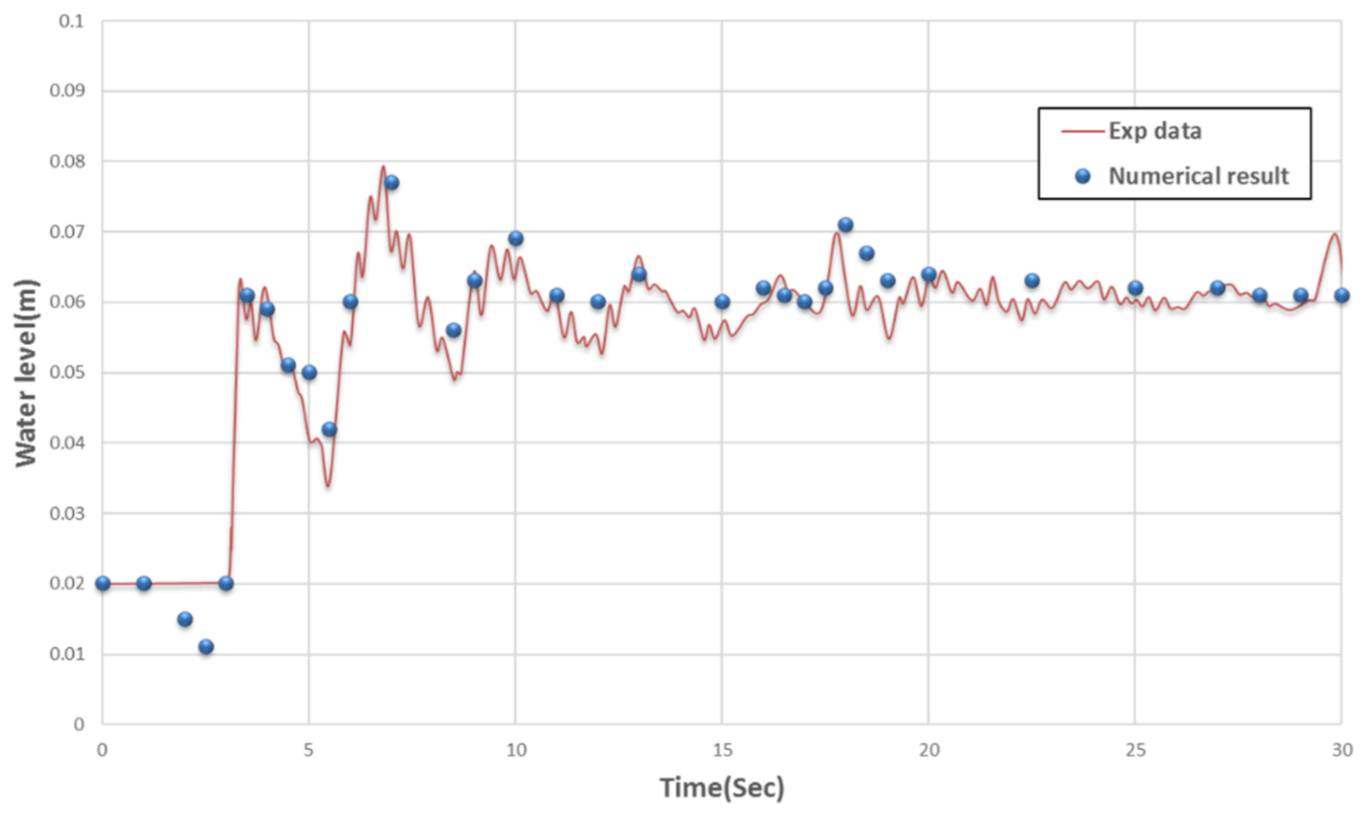
The numerical model results are compared with experimental data to verify the performance of the code. The experiments were carried out by Soares-Frazao in 2007 [40]. The length and width of the considered flume are 5.6 and 0.5 m, respectively. A sluice gate is placed at x = 2.39 with a reservoir depth of 0.111 m upstream. A symmetrical triangular barrier with 0.065 m height and ±0.14 slope on each side, at x = 4.45, is considered. The water depth of 0.02 m at the downstream side of the barrier is considered, and the other parts are assumed as dry (Figure 5).
By immediately opening the sluice gate, which simulates the breaking of the dam, three probes start measuring the water depth in different locations. In the numerical simulation, the no-slip condition is applied for all wall boundaries [22]. A total of 14,618 unstructured triangular cells are considered with a Manning roughness coefficient and Courant–Friedrichs–Lewy (CFL) number of 0.011 and 0.9, respectively. The water level fluctuation of G1 and G2 during the 10 and 30 s after the dam break is investigated to verify the numerical simulation. The results of the numerical modeling and the experimental results are shown in Figure 6 and Figure 7.
Conservation of Mass Verification
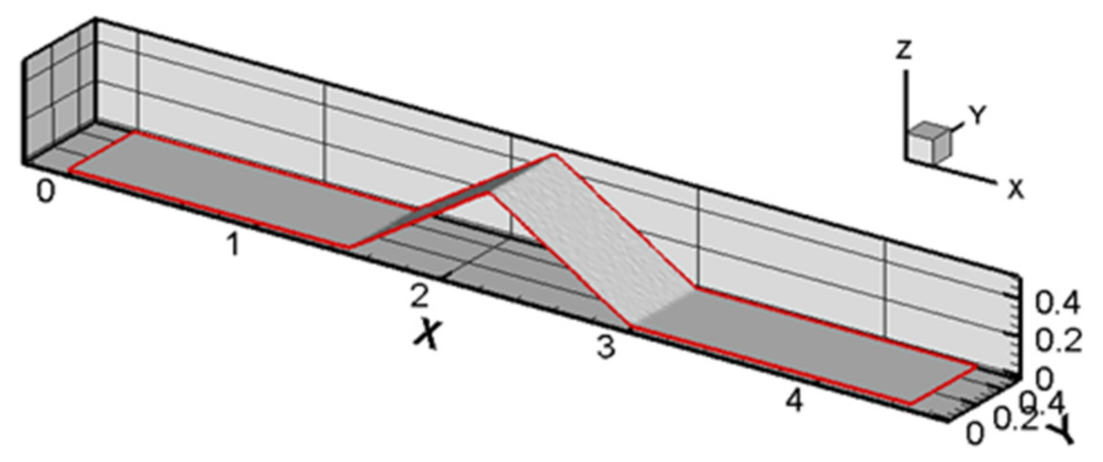
One of the crucial issues in every CFD numerical code is to check the continuity or conservation of mass. To verify the ability of the code to conserve the mass in a dry canal, a numerical wave tank (NWT) with a barrier is considered. The NWT is defined with a length and width of 4.5 and 0.5 m, respectively. A triangular barrier is modeled in the center of the canal with a base of 1.5 m, a height of 0.5 m and 0.5 m in width (Figure 8).
The computational domain is considered as 12120 unstructured triangular cells. The no-slip condition is applied for all wall boundaries [22]. The initial conditions are composed of a water column with a height of 2 m and a length of 1 m in which its width is equal to the canal’s width. The acceptable error of 10−8 is considered for the numerical code. Figure 9 shows the initial conditions of the test.
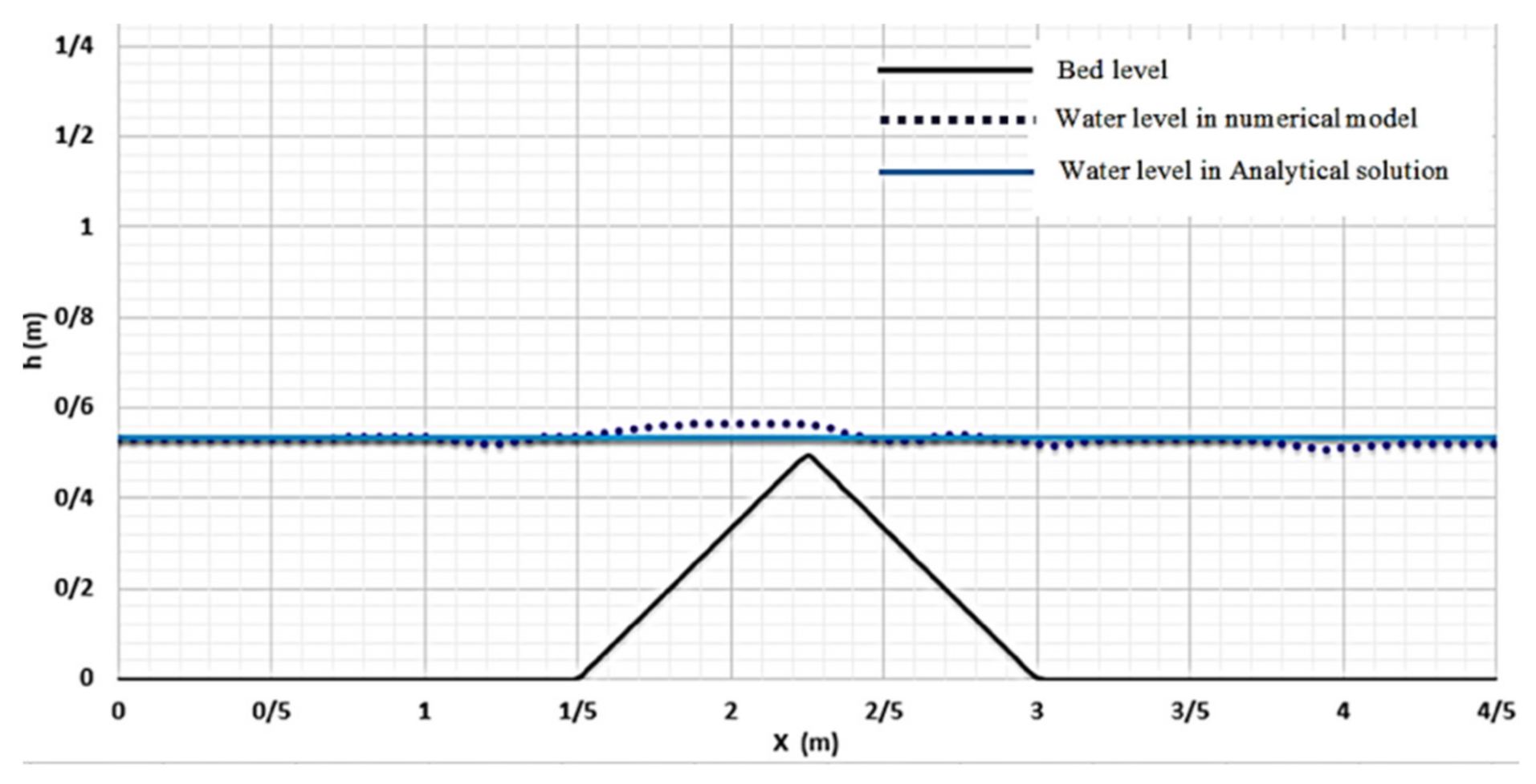
Figure 10 shows the flow passing through the barrier and the stability of water above the barrier at different time steps. The numerical test result is compared with the analytical method. In this regard, the volume of water and barrier volume are added together, and by dividing this volume with the solution domain, the water level after stability can be obtained. Table 1 presents the analytical solution and water level after stability.
Accordingly, the water level will be equal to 0.53 m along the canal after reaching the stable stage. Figure 11 shows numerical and analytical solution results in comparison. It is observed that numerical and analytical solution results are in good agreement, and the conservation of mass is preserved favorably.
5. Modeling of the Dam Break
The Golestan dam has been constructed on a river in the north of Iran. It has a length of 30.6 m at the bottom with a crest length of 130 m, it is 20 m in height, and its reservoir volume is 2.7 million cubic meters. The area of the watershed dam is 1,010,000 hectares. The Golestan dam is a historic barrier dating back 150 years that was built using traditional materials. This dam has been exposed to various earthquakes. The changing of the land use upstream of the dam has caused increasing water to enter it and increased the likelihood of failure. In this paper, the length of 5400 m of the river downstream of the dam has been modeled. The topography of the area, dam reservoir and pathway plan have been obtained. Figure 12 shows the river plan and land risks.
Two bridges, B1 and B2, are located at distances of 3900 m and 5320 m downstream of the dam, respectively. These two bridges are critical for the area, and the dam break could cause a serious problem for these bridges. Their properties are presented in Table 2.
Only bridge piers have been applied in the modeling, and due to the size of the computational domain, a slip condition has been used at the wall boundaries of the bridge piers [22]. At the downstream end, the dependent variables (h, qx and qy) were interpolated from the solution domain, which is reasonable due to the supercritical nature of the flow [39]. The Courant–Friedrichs–Lewy (CFL) number is considered as 0.8. Figure 13 shows a change of maximum flow depth with different numbers of computational cells at B1 and B2 bridges. According to this figure, 35,628 unstructured triangular cells were chosen.
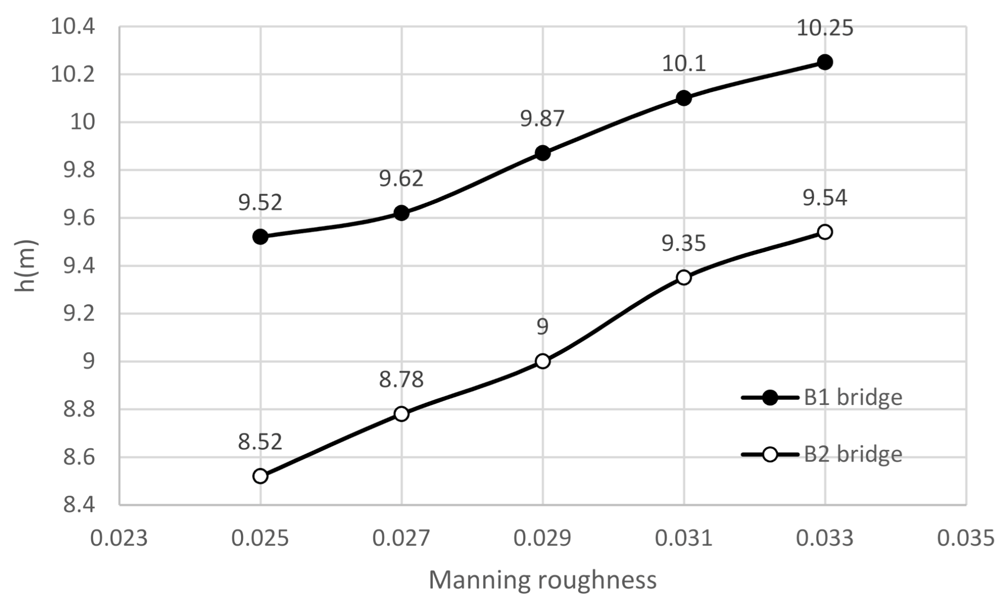
Due to the sand-bed river without vegetation downstream of the dam, the value of the Manning roughness coefficient varies between 0.025 and 0.033 [41]. The maximum depths of flood flow versus Manning roughness are shown in Figure 14 for the points attached to bridge B1 and B2. It is observed that with increasing Manning roughness from 0.025 to 0.033, the maximum depth of the flood wave increases by about 11%. For reliability, Manning roughness is considered as 0.033.
6. Results and Discussion
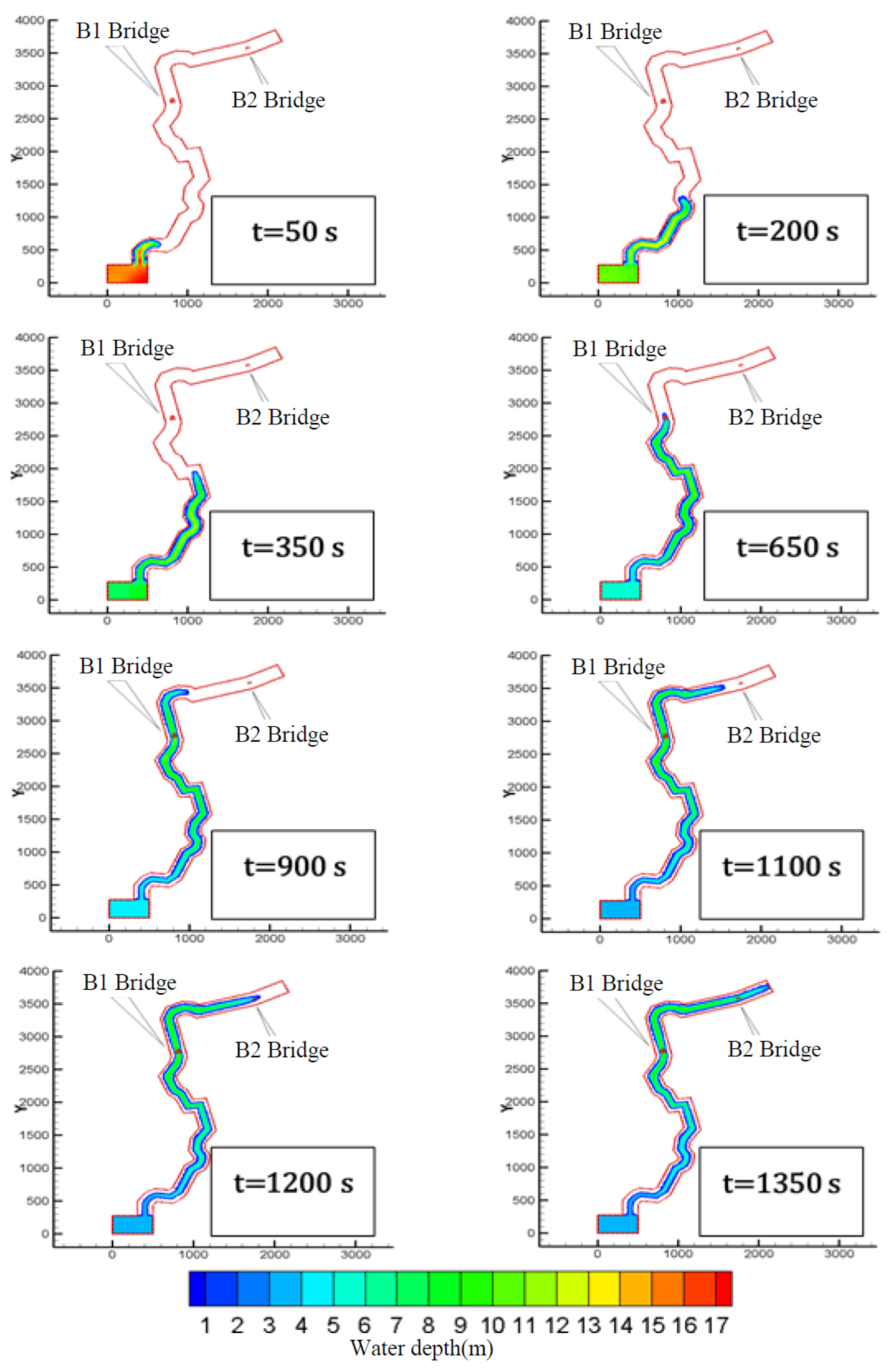
The dam break is simulated using the above information. The analysis continued up to the point where water level approaches the elevation of the bridge. The travel time duration of the first wave that hits the bridges is calculated. Figure 15 shows flood zoning in different periods. In this figure, the river border and computational domain are distinguished by red lines. Flood zoning indicates that water depth decreases gradually in the reservoir after the dam breaks, and it takes 22 min and 30 s.
Figure 14 and Figure 15 show a closer look at the flood wave when it arrives at the B1 bridge at a time of 620 and 660 s, respectively. The flow depth distribution across the river and the bridge’s piers are seen in Figure 16 and Figure 17.
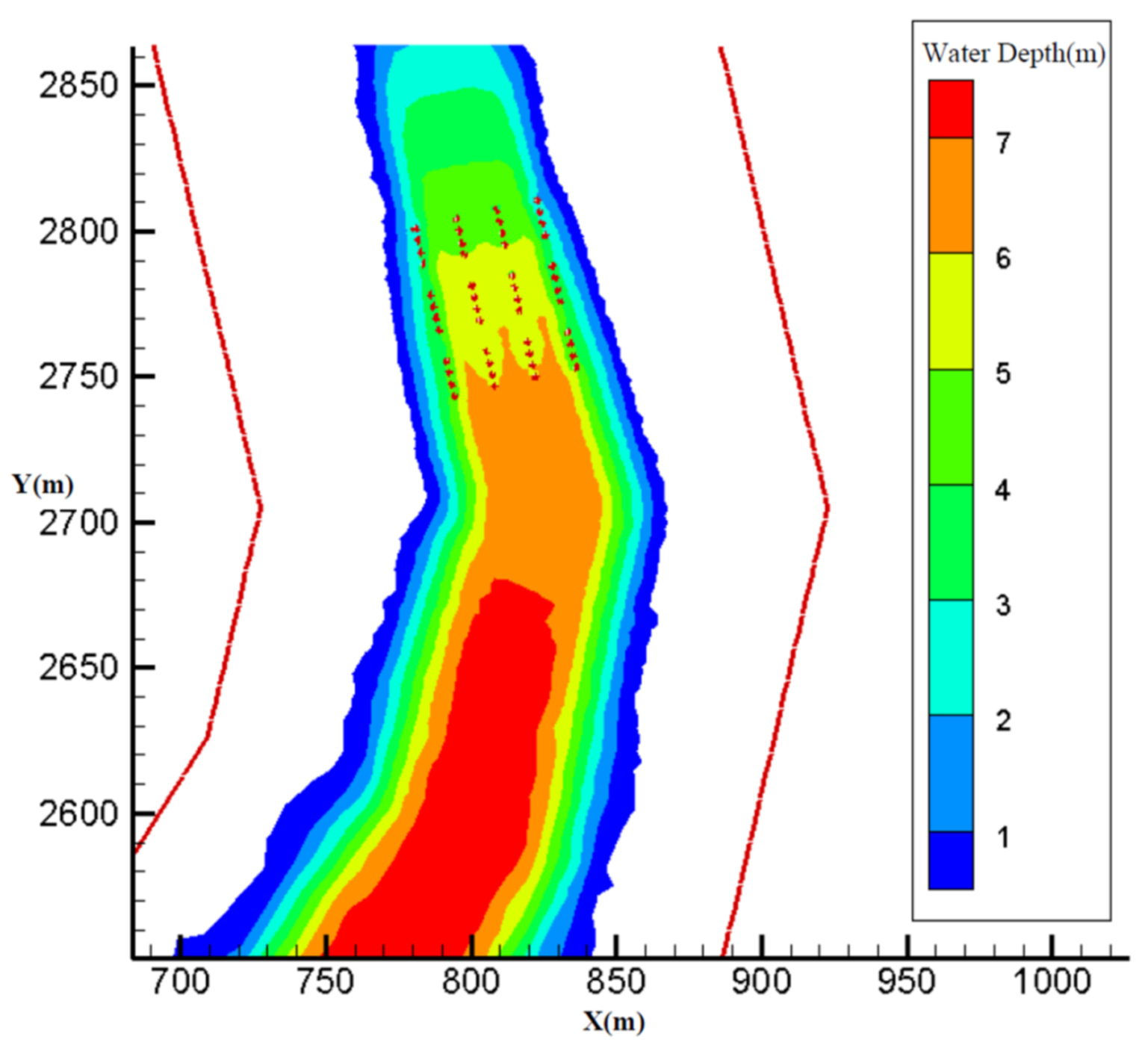
The velocity vectors and the contours of streamlines at the B1 bridge at time 1100 s are shown in Figure 18. According to this figure, the proper performance of the wall boundary condition is confirmed.
Flood flow hydrographs at bridges B1 and B2 are presented in Figure 19. It can be seen that the maximum flood discharge at the locations of bridges B1 and B2 is 120 (at time 16.5 min) and 110.2 (at time 28.5 min), respectively.
Figure 20 and Figure 21 present the water level at B1, B2 pier locations. The B1 deck bridge would suffer from flooding at 11 to 40 min after the break and encounter dangerous waves with greater heights than the deck bridge elevation. It is observed that the height of the waves reaches up to 4 m above deck bridge level, which could cause a disaster. According to Figure 20, it is observed that 11 min after the dam break, the height of the flood wave reaches the level of the bridge deck. Consequently, for this bridge, there are only 11 min after the breaking of the dam to apply necessary proceedings and evacuate the adjacent roads. Precautionary measures should be taken during the safe periods.
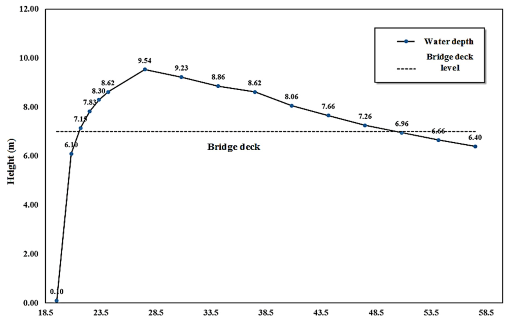
The results based on Figure 21 showed that the B2 bridge would be flooded from 21 to 50 min. The maximum wave height of 9.54 m will occur about 27 min after the breaking of the dam, which is 2.5 m greater than the bridge elevation. Therefore, for bridge B2, there is only 21 min available before the bridge is completely flooded, and road evacuation should be considered to prevent future risks.
7. Conclusions
Real-scale dam-break modeling using 3D numerical models has a high computational cost. It is very useful to use 2D models that can reduce the cost of calculations while being accurate. In this paper, a real-scale dam-break wave was simulated using the 2D finite volume Roe-TVD method. For this purpose, a numerical code was developed to solve the 2D depth average, shallow water equations on unstructured triangular cells considering turbulence terms and a dry bed front. In order to validate the code, at first, available experimental data were considered, the water level in the flume has been predicted and compared with the experimental data. Furthermore, a numerical tank was simulated to study the capability of the model in passing the flow over a barrier in the dry canal, conserving mass and to reach a steady flow case above the barrier level. Comparing the analytical and numerical solutions indicated that the conservation of mass is satisfied. After verifying the model, the real-scale dam break has been simulated, and the flow behavior from encountering the two bridges was analyzed along the pathway. The flood wave arrival time to the bridges, flooded area and the duration of flooding of the bridges were studied. The results of the dam break simulation showed that B1 and B2 bridges are at risk of flooding in the case of a dam break. Long waves affect the structures and can cause severe damage. Vehicle traffic should be banned at the moment of dam break. Furthermore, it is necessary to evacuate any vulnerable objects from these areas. The maximum required time for the evacuation of the two bridges is 12 and 21 min, respectively.
Author Contributions
Conceptualization, E.A.; methodology, E.A.; software, E.A.; validation, E.A., B.Đ. and S.D.; formal analysis, E.A., S.D. and B.Đ.; investigation, S.D. and E.A.; writing—original draft preparation, E.A.; visualization, E.A.; project administration, E.A. and B.Đ. All authors have read and agreed to the published version of the manuscript.
Funding
This research received no external funding.
Institutional Review Board Statement
Not applicable.
Informed Consent Statement
Not applicable.
Data Availability Statement
Data are available upon reasonable and unprofitable request.
Conflicts of Interest
The authors declare no conflict of interest.
References
- Wang, Z.; Shen, H.T. Lagrangian Simulation of One-Dimensional Dam-Break Flow. J. Hydraul. Eng. 1999, 125, 1217–1220. [Google Scholar] [CrossRef]
- Daneshfaraz, R.; Ghahramanzadeh, A.; Ghaderi, A.; Joudi, A.R.; Abraham, J. Investigation of the Effect of Edge Shape on Characteristics of Flow Under Vertical Gates. J. Am. Water Work. Assoc. 2016, 108, E425–E432. [Google Scholar] [CrossRef]
- Zoppou, C.; Roberts, S. Numerical solution of the two-dimensional unsteady dam break. Appl. Math. Model. 2000, 24, 457–475. [Google Scholar] [CrossRef]
- Bradford, S.F.; Sanders, B.F. Finite-volume model for shallow-water flooding of arbitrary topography. Appl. Math. Model. 2002, 128, 289–298. [Google Scholar]
- Valiani, A.; Caleffi, V.; Zanni, A. Case Study: Malpasset Dam-Break Simulation using a Two-Dimensional Finite Volume Method. J. Hydraul. Eng. 2002, 128, 460–472. [Google Scholar] [CrossRef]
- Ying, X.; Wang, S.S.Y.; Khan, A.A. Numerical Simulation of Flood Inundation due to Dam and Levee Breach. World Water Environ. Resour. Congr. 2003, 2003, 1–9. [Google Scholar] [CrossRef]
- Sanders, B.F.; Schubert, J.E.; Gallegos, H.A. Integral formulation of shallow-water equations with anisotropic porosity for urban flood modeling. J. Hydrol. 2008, 362, 19–38. [Google Scholar] [CrossRef]
- Ni, Y.; Cao, Z.; Borthwick, A.; Liu, Q. Approximate Solutions for Ideal Dam-Break Sediment-Laden Flows on Uniform Slopes. Water Resour. Res. 2018, 54, 2731–2748. [Google Scholar] [CrossRef]
- Fent, I.; Zech, Y.; Soares-Frazão, S. Dam-break flow experiments over mobile bed: Velocity profile. J. Hydraul. Res. 2018, 57, 131–138. [Google Scholar] [CrossRef]
- Park, K.M.; Yoon, H.S.; Kim, M.I. CFD-DEM based numerical simulation of liquid-gas-particle mixture flow in dam break. Commun. Nonlinear Sci. Numer. Simul. 2018, 59, 105–121. [Google Scholar] [CrossRef]
- Issakhov, A.; Zhandaulet, Y.; Nogaeva, A. Numerical simulation of dam break flow for various forms of the obstacle by VOF method. Int. J. Multiph. Flow 2018, 109, 191–206. [Google Scholar] [CrossRef]
- Yang, S.; Yang, W.; Qin, S.; Li, Q. Comparative study on calculation methods of dam-break wave. J. Hydraul. Res. 2018, 57, 702–714. [Google Scholar] [CrossRef]
- Shadloo, M.; Oger, G.; Le Touzé, D. Smoothed particle hydrodynamics method for fluid flows, towards industrial applications: Motivations, current state, and challenges. Comput. Fluids 2016, 136, 11–34. [Google Scholar] [CrossRef]
- Haltas, I.; Tayfur, G.; Elci, S. Two-dimensional numerical modeling of flood wave propagation in an urban area due to Ürkmez dam-break, İzmir, Turkey. Nat. Hazards 2016, 81, 2103–2119. [Google Scholar] [CrossRef] [Green Version]
- Medeiros, S.C.; Hagen, S.C. Review of wetting and drying algorithms for numerical tidal flow models. Int. J. Numer. Methods Fluids 2012, 71, 473–487. [Google Scholar] [CrossRef]
- Casulli, V.; Walters, R.A. An unstructured grid, three-dimensional model based on the shallow water equations. Int. J. Numer. Methods Fluids 2000, 32, 331–348. [Google Scholar] [CrossRef]
- Hou, J.; Simons, F.; Mahgoub, M.; Hinkelmann, R. A robust well-balanced model on unstructured grids for shallow water flows with wetting and drying over complex topography. Comput. Methods Appl. Mech. Eng. 2013, 257, 126–149. [Google Scholar] [CrossRef]
- Ji, Z.-G.; Morton, M.; Hamrick, J. Wetting and Drying Simulation of Estuarine Processes. Estuar. Coast. Shelf Sci. 2001, 53, 683–700. [Google Scholar] [CrossRef]
- Hamrick, J.M.; Mills, W.B. Analysis of water temperatures in Conowingo Pond as influenced by the Peach Bottom atomic power plant thermal discharge. Environ. Sci. Policy 2000, 3, 197–209. [Google Scholar] [CrossRef]
- Brufau, P.; Vázquez-Cendón, M.E.; García-Navarro, P. A numerical model for the flooding and drying of irregular domains. Int. J. Numer. Methods Fluids 2002, 39, 247–275. [Google Scholar] [CrossRef]
- Brufau, P.; Garcia-Navarro, P. Two-dimensional dam break flow simulation. Int. J. Numer. Methods Fluids 2000, 33, 35–57. [Google Scholar] [CrossRef]
- Cea, L.; Puertas, J.; Vázquez-Cendón, M.-E. Depth Averaged Modelling of Turbulent Shallow Water Flow with Wet-Dry Fronts. Arch. Comput. Methods Eng. 2007, 14, 303–341. [Google Scholar] [CrossRef]
- Song, L.; Zhou, J.; Li, Q.; Yang, X.; Zhang, Y. An unstructured finite volume model for dam-break floods with wet/dry fronts over complex topography. Int. J. Numer. Methods Fluids 2010, 67, 960–980. [Google Scholar] [CrossRef]
- Vichiantong, S.; Pongsanguansin, T.; Maleewong, M. Flood Simulation by a Well-Balanced Finite Volume Method in Tapi River Basin, Thailand, 2017. Model. Simul. Eng. 2019, 2019, 1–13. [Google Scholar] [CrossRef]
- do Carmo, J.S.A.; Ferreira, J.A.; Pinto, L. On the accurate simulation of nearshore and dam break problems involving dispersive breaking waves. Wave Motion 2019, 85, 125–143. [Google Scholar] [CrossRef]
- Do Carmo, J.A.; Ferreira, J.A.; Pinto, L.; Romanazzi, G. An improved Serre model: Efficient simulation and comparative evaluation. Appl. Math. Model. 2018, 56, 404–423. [Google Scholar] [CrossRef]
- Gallegos, H.A.; Schubert, J.E.; Sanders, B.F. Two-dimensional, high-resolution modeling of urban dam-break flooding: A case study of Baldwin Hills, California. Adv. Water Resour. 2009, 32, 1323–1335. [Google Scholar] [CrossRef]
- Spinewine, B.; Zech, Y. Small-scale laboratory dam-break waves on movable beds. J. Hydraul. Res. 2007, 45, 73–86. [Google Scholar] [CrossRef]
- Di Cristo, C.; Evangelista, S.; Greco, M.; Iervolino, M.; Leopardi, A.; Vacca, A. Dam-break waves over an erodible embankment: Experiments and simulations. J. Hydraul. Res. 2018, 56, 196–210. [Google Scholar] [CrossRef]
- Amicarelli, A.; Manenti, S.; Paggi, M. SPH Modelling of Dam-break Floods, with Damage Assessment to Electrical Substations. Int. J. Comput. Fluid Dyn. 2020, 1–19. [Google Scholar] [CrossRef]
- Dazzi, S.; Vacondio, R.; Mignosa, P. Internal boundary conditions for a GPU-accelerated 2D shallow water model: Implementation and applications. Adv. Water Resour. 2020, 137, 103525. [Google Scholar] [CrossRef]
- Ratia, H.; Murillo, J.; García-Navarro, P. Numerical modelling of bridges in 2D shallow water flow simulations. Int. J. Numer. Methods Fluids 2014, 75, 250–272. [Google Scholar] [CrossRef]
- USBR. Prediction of Embankment Dam Breach Parameters; Dam Safety Office: Denver, CO, USA, 1998.
- Costa, J. Floods from Dam Failures; US Geological Survey: Reston, VA, USA, 1985.
- Aliparast, M. Two-dimensional finite volume method for dam-break flow simulation. Int. J. Sediment Res. 2009, 24, 99–107. [Google Scholar] [CrossRef]
- Torabi, M.A.; Shafieefar, M. An experimental investigation on the stability of foundation of composite vertical breakwaters. J. Mar. Sci. Appl. 2015, 14, 175–182. [Google Scholar] [CrossRef]
- Shadloo, M.S. Numerical simulation of long wave runup for breaking and nonbreaking waves. Int. J. Offshore Polar Eng. 2015, 25, 1–7. [Google Scholar]
- Bermúdez, A.; Dervieux, A.; Desideri, J.-A.; Vázquez, M. Upwind schemes for the two-dimensional shallow water equations with variable depth using unstructured meshes. Comput. Methods Appl. Mech. Eng. 1998, 155, 49–72. [Google Scholar] [CrossRef] [Green Version]
- Alamatian, E.; Jaefarzadeh, M.R. Evaluation of turbulence models in simulation of oblique standing shock waves in supercritical channel flows. Sharif 2012, 28, 1–13. [Google Scholar] [CrossRef] [Green Version]
- Frazao, S.S. Experiments of dam-break wave over a triangular bottom sill. J. Hydraul. Res. 2007, 45, 19–26. [Google Scholar] [CrossRef]
- Ghani, A.A.; Zakaria, N.A.; Kiat, C.C.; Ariffin, J.; Hasan, Z.A.; Ghaffar, A.B. Revised equations for Manning’s coefficient for Sand-Bed Rivers. Int. J. River Basin Manag. 2007, 5, 329–346. [Google Scholar] [CrossRef] [Green Version]
Figure 1.
Finite volume cells [22]: (a) Initial triangle cell; (b) control volume.
Figure 1.
Finite volume cells [22]: (a) Initial triangle cell; (b) control volume.

Figure 2.
Flowchart of the written code.

Figure 3.
(a) A typical initial control volume cell. (b) Reconstruction of the conservative variables from the cell centers to the cell faces.
Figure 3.
(a) A typical initial control volume cell. (b) Reconstruction of the conservative variables from the cell centers to the cell faces.

Figure 4.
Discretization of the turbulent diffusion term.

Figure 5.
Geometrical properties of experimental model [40].
Figure 5.
Geometrical properties of experimental model [40].

Figure 6.
Water level variations at the station of G1 during the 30 s after dam break.

Figure 7.
Water level variations at the station of G2 during the 30 s after dam break.

Figure 8.
The geometry of the NWT in the test of flow passing barrier and stability above the barrier level.
Figure 8.
The geometry of the NWT in the test of flow passing barrier and stability above the barrier level.

Figure 9.
Initial conditions in the test of flow passing barrier and stability above the barrier level.
Figure 9.
Initial conditions in the test of flow passing barrier and stability above the barrier level.

Figure 10.
Progress of a wave in the test of flow passing the barrier and stability above the barrier level.
Figure 10.
Progress of a wave in the test of flow passing the barrier and stability above the barrier level.

Figure 11.
Numerical and analytical results in the test of flow passing barrier and stability above barrier level.
Figure 11.
Numerical and analytical results in the test of flow passing barrier and stability above barrier level.

Figure 12.
River plan and land risks.

Figure 13.
Maximum flow depth versus different numbers of computational cells.

Figure 14.
Maximum depths of flood flow versus Manning roughness.

Figure 15.
Flooded zoning due to the dam break.

Figure 16.
Water level at B1 bridge at time 620 s.

Figure 17.
Water level at B1 bridge at time 660 s.

Figure 18.
The velocity vectors and the contours of streamlines at the B1 bridge (t = 1100 s).

Figure 19.
Flood flow hydrographs at bridges B1 and B2.

Figure 20.
Water level variations at the B1 bridge.

Figure 21.
Water level variations at the B2 bridge.


Table 1.
Analytical solution and water level after stability.
| Properties | Water Volume (m3) | Barrier Volume (m3) | Total Volume of Barrier and Water (m3) | Domain Area (m2) | Water Level after Stability (m) |
|---|---|---|---|---|---|
| Values | 2 × 1 × 0.5 = 1 | [(0.5 × 1.5)/2] × 0.5 = 0.188 | 1 + 0.188 = 1.188 | 4.5 × 0.5 | 1.188/(4.5 × 0.5) = 0.53 |
Table 2.
Bridges Properties.
| Bridge Details | B1 Bridge | B2 Bridge |
|---|---|---|
| Pier radius | 0.6 m | 0.6 m |
| Number of piers | 48 | 16 |
| Bridge height | 6 m | 7 m |
Publisher’s Note: MDPI stays neutral with regard to jurisdictional claims in published maps and institutional affiliations. |
© 2021 by the authors. Licensee MDPI, Basel, Switzerland. This article is an open access article distributed under the terms and conditions of the Creative Commons Attribution (CC BY) license (https://creativecommons.org/licenses/by/4.0/).
Share and Cite
MDPI and ACS Style
Alamatian, E.; Dadar, S.; Đurin, B. Simulation of Dam Breaks on Dry Bed Using Finite Volume Roe-TVD Method. Hydrology 2021, 8, 88. https://0-doi-org.brum.beds.ac.uk/10.3390/hydrology8020088
AMA Style
Alamatian E, Dadar S, Đurin B. Simulation of Dam Breaks on Dry Bed Using Finite Volume Roe-TVD Method. Hydrology. 2021; 8(2):88. https://0-doi-org.brum.beds.ac.uk/10.3390/hydrology8020088
Chicago/Turabian StyleAlamatian, Ebrahim, Sara Dadar, and Bojan Đurin. 2021. "Simulation of Dam Breaks on Dry Bed Using Finite Volume Roe-TVD Method" Hydrology 8, no. 2: 88. https://0-doi-org.brum.beds.ac.uk/10.3390/hydrology8020088
Note that from the first issue of 2016, this journal uses article numbers instead of page numbers. See further details here.