
Numerical and Experimental Approaches to Estimate Discharge Coefficients and Energy Loss Coefficients in Pressurized Grated Inlets


Abstract
:1. Introduction
2. Materials and Methods
2.1. Experimental Set-Up
2.2. Data Collection
2.3. Numerical Simulation
2.3.1. Numerical Model
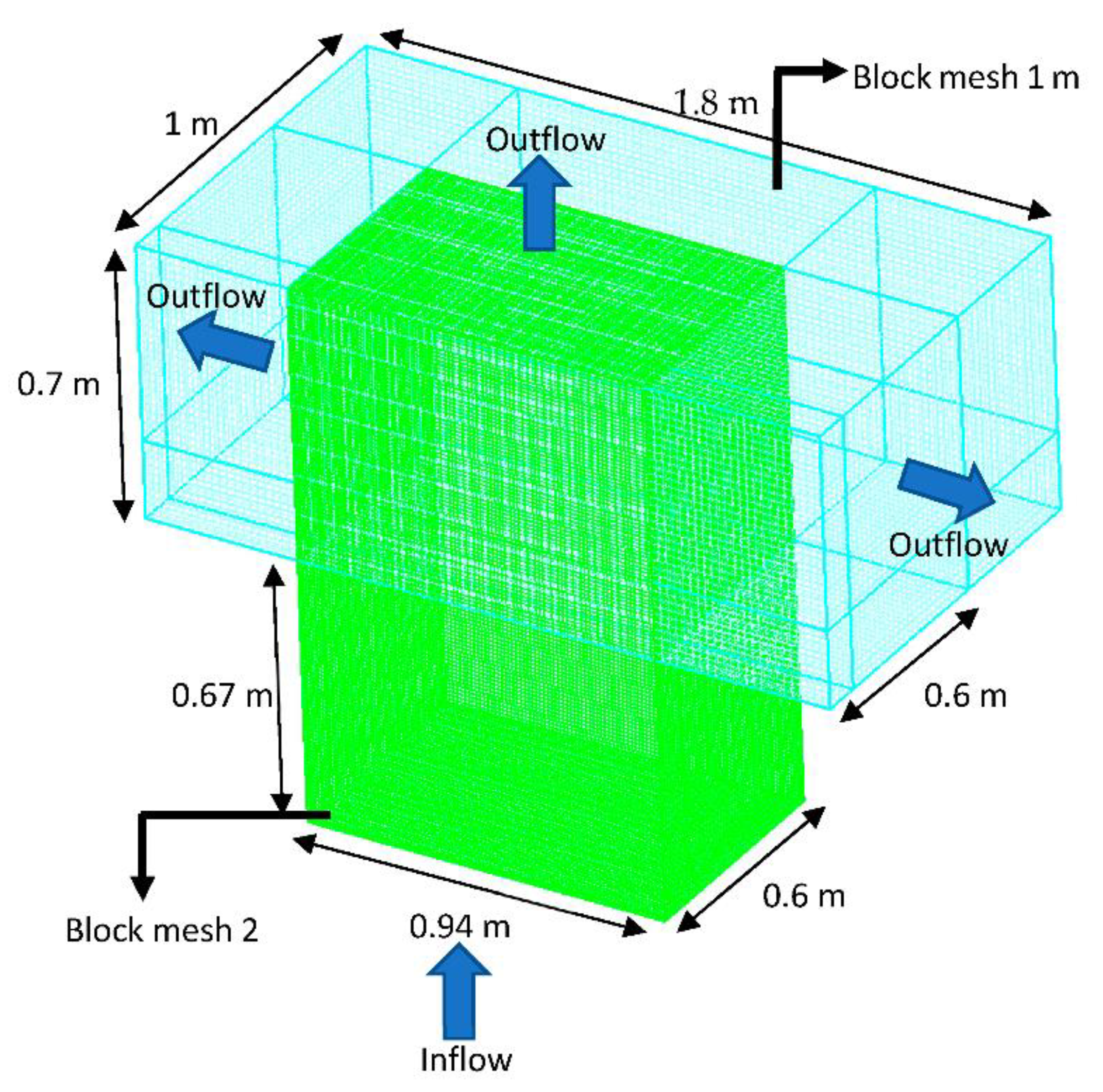
2.3.2. Pre-Processing
2.3.3. Post-Processing
3. Results
4. Conclusions
Author Contributions
Funding
Institutional Review Board Statement
Informed Consent Statement
Data Availability Statement
Conflicts of Interest
References
- Ashley, M.R.; Balmfort, D.J.; Saul, A.J.; Blanksy, D.J. Flooding in the future- predicting climate change, risks and responses in urban areas. Water Sci. Technol. 2005, 52, 265–273. [Google Scholar]
- Un.org. World’s Population Increasingly Urban with More than Half Living in Urban Areas | UN DESA | United Nations Department of Economic and Social Affairs. 2014. Available online: http://www.un.org/en/development/desa/news/population/world-urbanization-prospects-2014.html (accessed on 2 January 2019).
- Ortiz, A.; Velasco, M.J.; Esbri, O.; Medina, V.; Russo, B. The economic impact of climate change on urban drainage master planning in Barcelona. Sustainability 2021, 13, 71. [Google Scholar] [CrossRef]
- Russo, B.; Velasco, M.; Locatelli, L.; Sunyer, D.; Yubero, D.; Monjo, R.; Martínez-Gomariz, E.; Forero-Ortiz, E.; Sánchez-Muñoz, D.; Evans, B.; et al. Assessment of urban flood resilience in Barcelona for current and future scenarios. The RESCCUE Project. Sustainability 2020, 12, 5638. [Google Scholar] [CrossRef]
- Russo, B.; Velasco, M.; Monjo, R.; Martínez-Gomariz, E.; Domínguez, J.L.; Sánchez, D.; Gabàs, A.; Gonzalez, A. Assessment of the resilience of Barcelona urban services in case of flooding. The RESCCUE project. Ingeniería del Agua 2020, 24, 101–118. [Google Scholar] [CrossRef]
- Brown, R.R. Impediments to integrated urban stormwater management: The need for institutional reform. Environ. Manag. 2005, 36, 455–468. [Google Scholar]
- Martins, R.; Leandro, J.; Djordjevic, S. Influence of sewer network models on urban flood damage assessment based on coupled 1D/2D models. J. Flood Risk Manag. 2016, 11, S717–S728. [Google Scholar] [CrossRef]
- De St Venant, B. Théorie du mouvement non permanent des eaux, avec application aux crues des rivières et a l’introduction de marées dans leurs lits. Comptes Rendus L’académie Sci. 1981, 73, 148–154. [Google Scholar]
- Russo, B.; Sunyer, D.; Velasco, M.; Djordjević, S. Analysis of extreme flooding events through a calibrated 1D/2D coupled model: The case of Barcelona (Spain). J. Hydroinform. 2015, 17, 473–491. [Google Scholar] [CrossRef]
- Valentin, M.G.; Macchione, F.; Russo, B. Comportamiento hidráulico de las calles durante lluvias extremas en zonas urbanas. Ing. Hidráulica México 2009, 24, 51–62. [Google Scholar]
- Martínez-Gomariz, E.; Gómez, M.; Russo, B.; Sánchez, P.; Montes, J.A. Damage assessment methodology for vehicles exposed to flooding in urban areas. Ingeniería del Agua 2017, 21, 247–262. [Google Scholar] [CrossRef] [Green Version]
- Rubinato, M.; Martins, R.; Shucksmith, J.D. Quantification of energy losses at a surcharging manhole. Urban Water J. 2018, 15, 234–241. [Google Scholar] [CrossRef] [Green Version]
- Cosco, C.; Gómez, M.; Russo, B.; Tellez-Alvarez, J.; Macchione, F.; Costabile, P.; Costanzo, C. Discharge coefficients for specific grated inlets. Influence of the Froude number. Urban Water J. 2020, 17, 656–668. [Google Scholar] [CrossRef]
- Tellez-Alvarez, J.; Gómez, M.; Russo, B. Quantification of energy loss in two grated inlets under pressure. Water 2020, 12, 1601. [Google Scholar] [CrossRef]
- Gómez, M.; Russo, B.; Tellez-Alvarez, J. Experimental investigation to estimate the discharge coefficient of a grate inlet under surcharge conditions. Urban Water J. 2019, 16, 85–91. [Google Scholar] [CrossRef]
- Gómez, M.; Russo, B. Methodology to estimate hydraulic efficiency of drain inlets. Water Manag. 2011, 164, 81–90. [Google Scholar] [CrossRef]
- Saul, A.; Djordjevic, S.; Maksimovic, C.; Blanksby, J. Flood Risk Science and Management; Wiley-Blackwell: Hoboken, NJ, USA, 2011; pp. 258–291. [Google Scholar]
- Djordjević, S.; Prodanović, D.; Maksimović, Č.; Ivetić, M.; Savić, D. SIPSON—Simulation of interaction between pipe flow and surface overland flow in networks. Water Sci. Technol. 2005, 52, 275–283. [Google Scholar] [PubMed]
- Glenis, V.; McGough, A.S.; Kutija, V.; Kilsby, C.; Woodman, S. Flood modelling for cities using Cloud computing. J. Cloud Comput. Adv. Syst. Appl. 2013, 2, 7. [Google Scholar] [CrossRef] [Green Version]
- Bertsch, R.; Glenis, V.; Kilsby, C. Urban flood simulation using synthetic storm drain networks. Water 2017, 9, 925. [Google Scholar] [CrossRef] [Green Version]
- Nones, M.; Caviedes-Voullième, D. Computational advances and innovations in flood risk mapping. J. Flood Risk Manag. 2020, 13, e12666. [Google Scholar] [CrossRef]
- Sampson, C.C.; Fewtrell, T.J.; Duncan, A.; Shaad, K.; Horritt, M.S.; Bates, P.D. Use of terrestrial laser scanning data to drive decimetric resolution urban inundation models. Adv. Water Resour. 2012, 41, 1–17. [Google Scholar] [CrossRef]
- Bach, P.M.; Rauch, W.; Mikkelsen, P.S.; McCarthy, D.; Deletic, A. A critical review of integrated urban water modelling—Urban drainage and beyond. Environ. Model. Softw. 2014, 54, 88–107. [Google Scholar] [CrossRef]
- Rubinato, M.; Lee, S.; Martins, R.; Shucksmith, J.D. Surface to sewer flow exchange through circular inlets during urban flood conditions. J. Hydroinform. 2018, 20, 564–576. [Google Scholar] [CrossRef] [Green Version]
- Rubinato, M.; Martins, R.; Kesserwani, G.; Leandro, J.; Djordjević, S.; Shucksmith, J. Experimental calibration and validation of sewer/surface flow exchange equations in steady and unsteady flow conditions. J. Hydrol. 2017, 552, 421–432. [Google Scholar] [CrossRef]
- Kidd, C.H.R.; Helliwell, P.R. Simulation of the inlet hydrograph for urban catchments. J. Hydrol. 1977, 35, 159–172. [Google Scholar] [CrossRef]
- Djordjević, S.; Prodanović, D.; Maksimović, Č. An approach to simulation of dual drainage. Water Sci. Technol. 1999, 39, 95–103. [Google Scholar] [CrossRef]
- Obermayer, A.; Guenthert, F.W.; Angermair, G.; Tandler, R.; Braunschmidt, S.; Milojevic, N. Different approaches for modelling of sewer caused urban flooding. Water Sci. Technol. 2010, 62, 2175–2182. [Google Scholar] [CrossRef] [PubMed]
- Schmitt, T.G.; Thomas, M.; Ettrich, N. Analysis and modeling of flooding in urban drainage systems. J. Hydrol. 2004, 299, 300–311. [Google Scholar] [CrossRef]
- Dai, S.; Jin, S.; Qian, C.; Yang, N.; Ma, Y.; Liang, C. Interception efficiency of grate inlets for sustainable urban drainage systems design under different road slopes and approaching discharges. Urban Water J. 2021, 18, 650–661. [Google Scholar] [CrossRef]
- Ettrich, N.; Steiner, K.; Thomas, M.; Rothe, R. Surface models for coupled modelling of runoff and sewer flow in urban areas. Water Sci. Technol. 2005, 52, 25–33. [Google Scholar] [CrossRef]
- Mark, O.; Weesakul, S.; Apirumanekul, C.; Aroonnet, S.B.; Djordjević, S. Potential and limitations of 1D modelling of urban flooding. J. Hydrol. 2004, 299, 284–299. [Google Scholar] [CrossRef]
- Nasello, C.; Tucciarelli, T. Dual multilevel urban drainage model. J. Hydraul. Eng. 2005, 131, 748–754. [Google Scholar] [CrossRef]
- Hunter, N.M.; Bates, P.D.; Neelz, S.; Pender, G.; Villanueva, I.; Wright, N.G.; Liang, D.; Falconer, R.A.; Lin, B.; Wallwe, S.; et al. Benchmarking 2D hydraulic models for urban flooding. Water Manag. 2008, 161, 13–30. [Google Scholar]
- Vojinovic, Z.; Seyoum, S.D.; Mwalwaka, J.M.; Price, R.K. Effects of model schematisation, geometry and parameter values on urban flood modelling. Water Sci. Technol. 2011, 63, 462–467. [Google Scholar] [CrossRef]
- Mason, D.C.; Horritt, M.S.; Hunter, N.M.; Bates, P.D. Use of fused airborne scanning laser altimetry and digital map data for urban flood modelling. Hydrol. Process. 2007, 21, 1436–1447. [Google Scholar] [CrossRef]
- Gibson, M.J.; Savic, D.A.; Djordjevic, S.; Chen, A.S.; Fraser, S.; Watson, T. Accuracy and computational efficiency of 2D urban surface flood modelling based on cellular automata. Procedia Eng. 2016, 154, 801–810. [Google Scholar] [CrossRef] [Green Version]
- Chen, Y.; Han, D. On big data and hydroinformatics. Procedia Eng. 2016, 154, 184–191. [Google Scholar] [CrossRef] [Green Version]
- Russo, B.; Gomez, M.; Martinez, P.; Sanchez, H. Methodology to study the surface runoff in urban streets and the design inlets systems. Application in a real case study. In Proceedings of the 10th International Conference on Urban Drainage, Copenhagen, Denmark, 21–26 August 2005. [Google Scholar]
- Pandit, S.K.; Oka, Y.; Shigeta, N.; Watanabe, M. Comparative efficiencies study of slot model and mouse model in pressurised pipe flow. J. Urban Environ. Eng. 2014, 8, 83–88. [Google Scholar] [CrossRef]
- Preissmann, A. Propagation des intumescences dans les canaux et rivières. In Proceedings of the First Congress of the French Association for Computation, Grenoble, France, September 1961. [Google Scholar]
- Djordjević, S.; Saul, A.J.; Tabor, G.; Blanksby, J.; Galambos, I.; Sabtu, N.; Sailor, G. Experimental and numerical investigation of interactions between above and below ground drainage systems. Water Sci. Technol. 2013, 67, 535–542. [Google Scholar] [CrossRef]
- Bazin, P.-H.; Nakagawa, H.; Kawaike, K.; Paquier, A.; Mignot, E. Modeling flow exchanges between a street and an underground drainage pipe during urban floods. J. Hydraul. Eng. 2014, 140, 04014051. [Google Scholar] [CrossRef]
- Butler, D.; Davies, J.W. Urban Drainage; Spon Press: London, UK; New York, NY, USA, 2011. [Google Scholar]
- Neenah Foundry Company (NFCO). Inlet Spacing Calculators, Website Applications; Neenah Foundry Company (NFCO): Neenah, WI, USA, 2021. [Google Scholar]
- Russo, B.; Gómez, M.; Macchione, F. Pedestrian hazard criteria for flooded urban areas. Nat. Hazards 2013, 69, 251–265. [Google Scholar] [CrossRef]
- Martínez-Gomariz, E.; Gómez, M.; Russo, B. Experimental study of the stability of pedestrians exposed to urban pluvial flooding. Nat. Hazards 2016, 82, 1259–1278. [Google Scholar] [CrossRef] [Green Version]
- Martínez-Gomariz, E.; Gómez, M.; Russo, B.; Djordjević, S. A new experiments-based methodology to define the stability threshold for any vehicle exposed to flooding. Urban Water J. 2017, 14, 930–939. [Google Scholar] [CrossRef]
- Martínez-Gomariz, E.; Gómez, M.; Russo, B.; Djordjević, S. Stability criteria for flooded vehicles: A state-of-the-art review. J. Flood Risk Manag. 2016, 11, S817–S826. [Google Scholar] [CrossRef]
- Russo, B.; Gómez, M.; Tellez, J.; Tellez-Alvarez, J. Methodology to estimate the hydraulic efficiency of nontested continuous transverse grates. J. Irrig. Drain. Eng. 2013, 139, 864–871. [Google Scholar] [CrossRef]
- Tellez-Alvarez, J. Image Processing and Experimental Techniques to Characterize the Hydraulic Performance of Grate Inlet. Ph.D. Thesis, Technical University of Catalonia, Barcelona, Spain, 2019. [Google Scholar]
- Gómez, M.; Sánchez, H.; Malgrat, P.; Castillo, F. Inlet spacing considering the risk associated to runoff: Application to streets and critical points of the City of Barcelona. In Proceedings of the 9th International Conference on Urban Drainage, (ICUD), Barcelona, Spain, 8–13 September 2002. [Google Scholar]
- Amezaga-Kutija, M. Assessment of the Discharge Coefficient for a Surcharging Inlet: Numerical and Experimental Comparison. Master’s Thesis, Civil Engineering Degree, University of Sheffield, Sheffield, UK, 2019. [Google Scholar]
- Flow 3D Version 12.0 Users Manual, Flow 3D (Computer Software); Flow Science, Inc.: Santa Fe, NM, USA, 2019.
- Gómez, M.; Recasens, J.; Russo, B.; Martínez-Gomariz, E. Assessment of inlet efficiency through a 3D simulation: Numerical and experimental comparison. Water Sci. Technol. 2016, 74, 1926–1935. [Google Scholar] [CrossRef] [Green Version]
- Russo, B.; Valentín, M.; Tellez-Álvarez, J. The relevance of grated inlets within surface drainage systems in the field of urban flood resilience. A review of several experimental and numerical simulation approaches. Sustainability 2021, 13, 7189. [Google Scholar] [CrossRef]
- Tellez-Alvarez, J.D.; Gómez, M.; Russo, B. Modelling of surcharge flow through grated inlet. In Advances in Hydroinformatics; Springer: Berlin/Heidelberg, Germany, 2020; pp. 839–847. [Google Scholar] [CrossRef]
- Bayon, A.; Valero, D.; García-Bartual, R.; Vallés-Morán, F.; López-Jiménez, P.A. Performance assessment of OpenFOAM and FLOW-3D in the numerical modeling of a low Reynolds number hydraulic jump. Environ. Model. Softw. 2016, 80, 322–335. [Google Scholar] [CrossRef]
- Morovati, K.; Eghbalzadeh, A. Study of inception point, void fraction and pressure over pooled stepped spillways using Flow-3D. Int. J. Numer. Methods Heat Fluid Flow 2018, 28, 982–998. [Google Scholar] [CrossRef]


| Cell Size (cm) | Time (mins) | Total Number of Cells (Unit) |
|---|---|---|
| 0.5 | 920 | 25,292,512 |
| 0.75 | 139 | 772,701 |
| 1 | 25 | 324,064 |
| 1.25 | 11 | 164,240 |
| 1.5 | 5 | 94,875 |
| 2 | 2 | 40,508 |
| 3 | 0.8 | 12,285 |
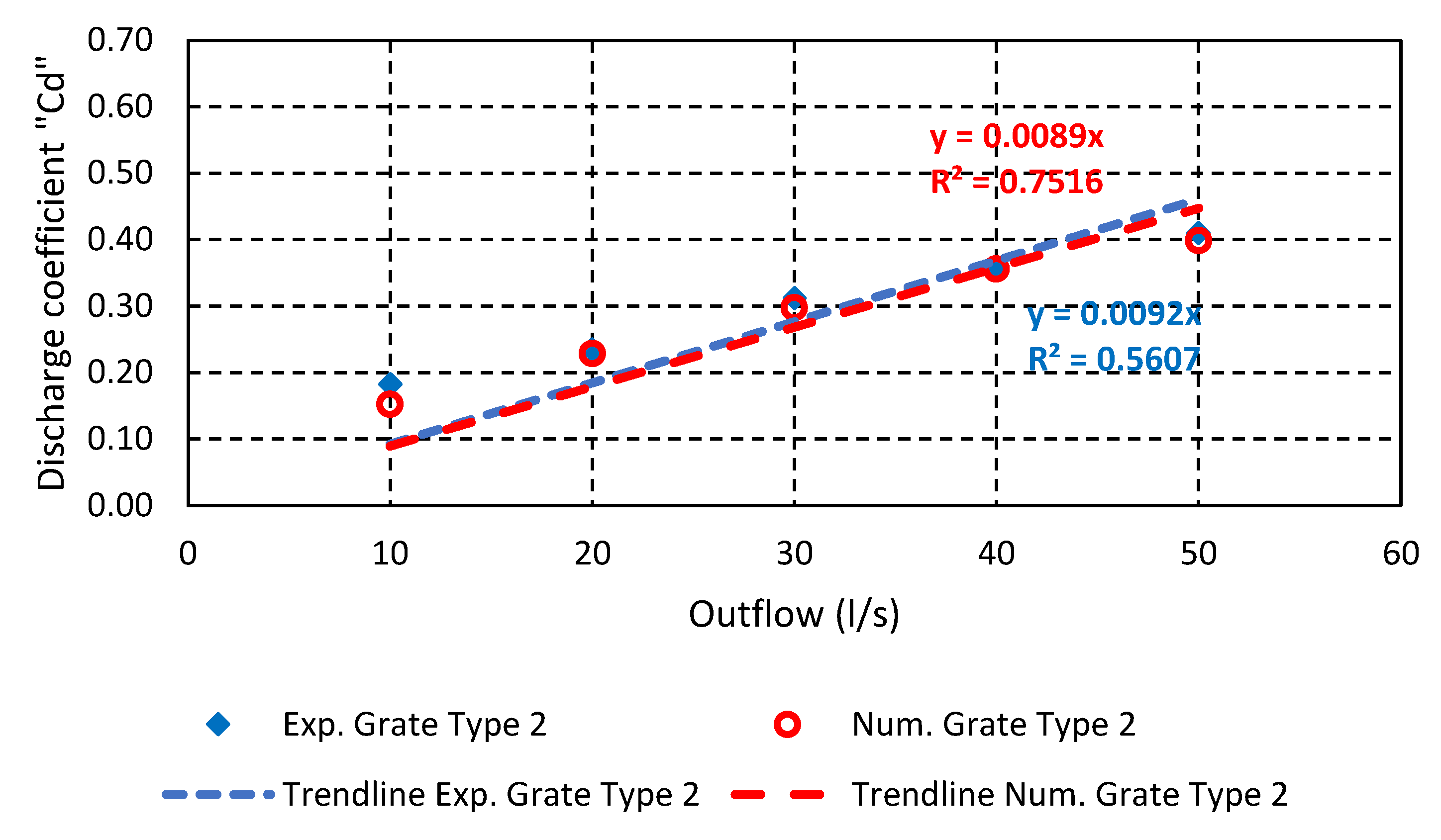
| Flowrate (l/s) | Grate Type 1 Exp. Cd | Grate Type 1 Num. Cd | Grate Type 2 Exp. Cd | Grate Type 2 Num. Cd | Grate Type 3 Num. Cd |
|---|---|---|---|---|---|
| 10 | 0.14 | 0.15 | 0.18 | 0.15 | 0.18 |
| 20 | 0.22 | 0.22 | 0.23 | 0.23 | 0.26 |
| 30 | 0.29 | 0.29 | 0.31 | 0.30 | 0.34 |
| 40 | 0.36 | 0.36 | 0.36 | 0.36 | 0.42 |
| 50 | 0.41 | 0.40 | 0.41 | 0.40 | 0.46 |
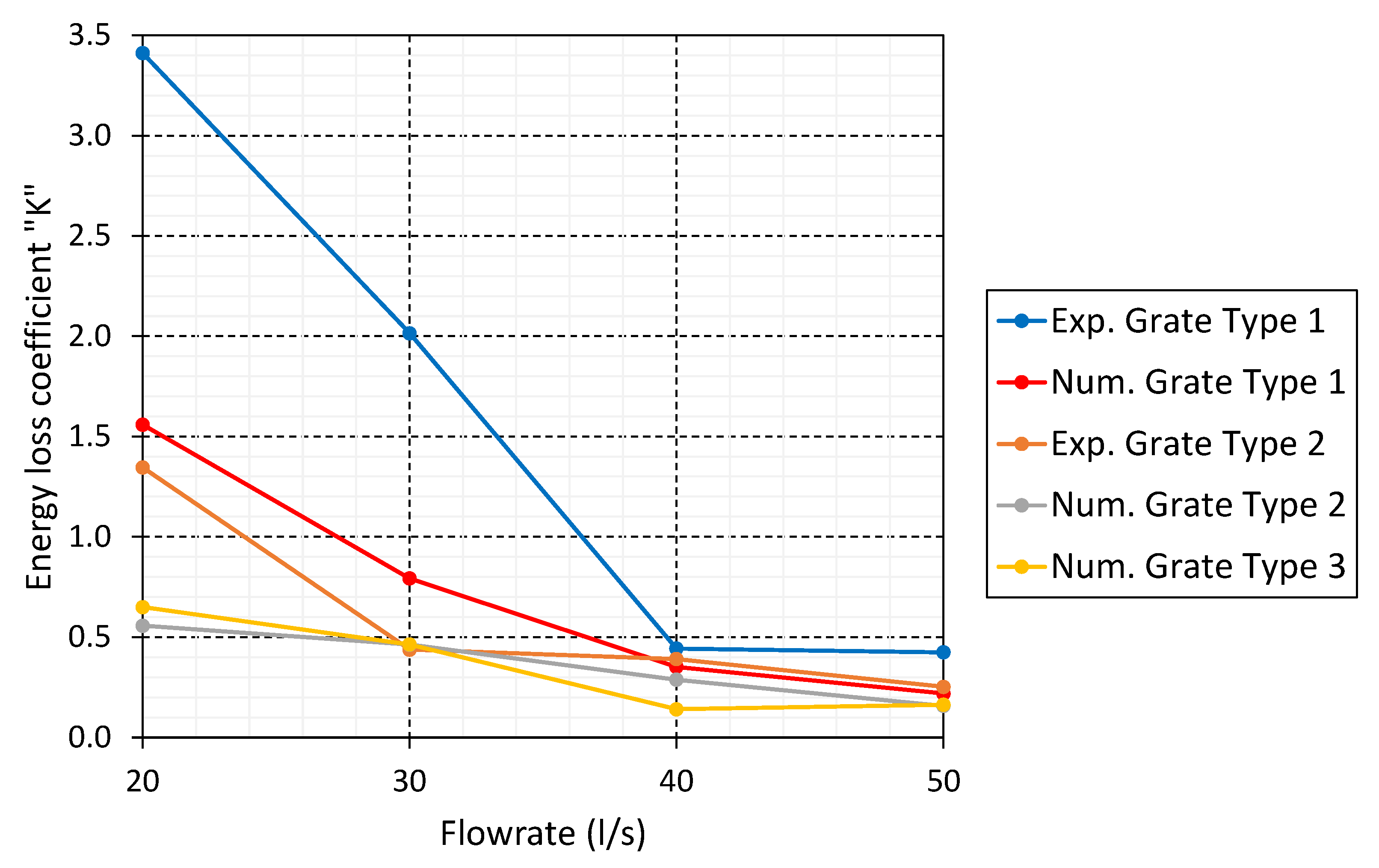
| Flowrate (l/s) | Grate Type 1 Exp. k | Grate Type 1 Num. k | Grate Type 2 Exp. k | Grate Type 2 Num. k | Grate Type 3 Num. k |
|---|---|---|---|---|---|
| 20 | 3.41 | 1.56 | 1.35 | 0.56 | 0.65 |
| 30 | 2.02 | 0.79 | 0.44 | 0.49 | 0.46 |
| 40 | 0.44 | 0.35 | 0.39 | 0.29 | 0.14 |
| 50 | 0.42 | 0.22 | 0.25 | 0.15 | 0.16 |
Publisher’s Note: MDPI stays neutral with regard to jurisdictional claims in published maps and institutional affiliations. |
© 2021 by the authors. Licensee MDPI, Basel, Switzerland. This article is an open access article distributed under the terms and conditions of the Creative Commons Attribution (CC BY) license (https://creativecommons.org/licenses/by/4.0/).
Share and Cite
Tellez-Alvarez, J.; Gómez, M.; Russo, B.; Amezaga-Kutija, M. Numerical and Experimental Approaches to Estimate Discharge Coefficients and Energy Loss Coefficients in Pressurized Grated Inlets. Hydrology 2021, 8, 162. https://0-doi-org.brum.beds.ac.uk/10.3390/hydrology8040162
Tellez-Alvarez J, Gómez M, Russo B, Amezaga-Kutija M. Numerical and Experimental Approaches to Estimate Discharge Coefficients and Energy Loss Coefficients in Pressurized Grated Inlets. Hydrology. 2021; 8(4):162. https://0-doi-org.brum.beds.ac.uk/10.3390/hydrology8040162
Chicago/Turabian StyleTellez-Alvarez, Jackson, Manuel Gómez, Beniamino Russo, and Marko Amezaga-Kutija. 2021. "Numerical and Experimental Approaches to Estimate Discharge Coefficients and Energy Loss Coefficients in Pressurized Grated Inlets" Hydrology 8, no. 4: 162. https://0-doi-org.brum.beds.ac.uk/10.3390/hydrology8040162