
Quantifying Groundwater Resources for Municipal Water Use in a Data-Scarce Region


Department of Engineering, University of Messina, Villaggio S. Agata, 98166 Messina, Italy
*
Author to whom correspondence should be addressed.
Hydrology 2021, 8(4), 184; https://0-doi-org.brum.beds.ac.uk/10.3390/hydrology8040184
Submission received: 24 November 2021
/
Revised: 13 December 2021
/
Accepted: 14 December 2021
/
Published: 16 December 2021
(This article belongs to the Special Issue Soil Water Balance)
Abstract
:Groundwater is a major source of drinking water worldwide, often considered more reliable than surface water and more accessible. Nowadays, there is wide recognition by the scientific community that groundwater resources are under threat from overexploitation and pollution. Furthermore, frequent and prolonged drought periods due to climate change can seriously affect groundwater recharge. For an appropriate and sustainable management of water systems supplied by springs and/or groundwater withdrawn from aquifers through drilling wells or drainage galleries, the need arises to properly quantify groundwater resources availability, mainly at the monthly scale, as groundwater recharge is influenced by seasonality, especially in the Mediterranean areas. Such evaluation is particularly important for ungauged groundwater bodies. This is the case of the aquifer supplying the Santissima Aqueduct, the oldest water supply infrastructure of the city of Messina in Sicily (Southern Italy), whose groundwater flows are measured only occasionally through spring water sampling at the water abstraction plants. Moreover, these plants are barely maintained because they are difficult to reach. In this study, groundwater recharge assessment for the Santissima Aqueduct is carried out through a GIS-based inverse hydrogeological balance methodology. Although this approach was originally designed to assess aquifer recharge at the annual scale, wherever a model conceptualization of the groundwater system was hindered by the lack of data, in the present study some changes are proposed to adjust the model to the monthly scale. In particular, the procedure for evapotranspiration assessment is based on the Global Aridity Index within the Budyko framework. The application of the proposed methodology shows satisfactory results, suggesting that it can be successfully applied for groundwater resources estimation in a context where monthly information is relevant for water resources planning and management.
1. Introduction
Groundwater-fed pipe systems for drinking water supply are widely used infrastructures. These systems rely on aquifers, whose recharge is mainly driven by precipitation, complemented by natural infiltration by surface water or by artificial recharge.
Modifications in the precipitation and temperature regimes due to climate change, as well as additional influences, such as land-use changes and groundwater abstractions, can alter groundwater level, storage, or discharge [1].
On the one hand, increased precipitation intensity may decrease groundwater recharge owing to the exceedance of the infiltration capacity (typically in humid areas) or may increase it because of faster percolation through the root zone and thus reduced evapotranspiration (typically in semiarid areas) [2,3]. On the other hand, growing urbanization and irrigation can play a significant role by respectively decreasing and increasing groundwater recharge [4,5].
To this end, a systematic quantification of the aquifers’ recharge is a relevant factor for water resources planning and management in such systems.
The direct quantification of aquifer recharge is a difficult task largely because recharge rates vary greatly in space and time, and thus direct measurements can only be obtained at the plot scale, for instance, from lysimeters [6,7,8]. For groundwater recharge estimation, many different methods and techniques have been developed over the years and intensively discussed in the literature [9,10,11,12] The different approaches mainly depend on the availability of data and the required level of accuracy [13], as well as on the sources and mechanisms of recharge [11].
At the regional scale, numerical modeling approaches are usually applied to assess recharge and the relationships between climate, land-use changes, and recharge [14] and references therein. The level of complexity of these models can vary from very simplified to very detailed physically-based models.
An example of the first type is represented by the model IHACRES (Identification of unit Hydrographs And Component flows from Rainfall, Evaporation and Streamflow data) [15] and further modifications to explicitly take into account the groundwater component [16,17,18]. Among complex numerical models, MODFLOW (MODular three-dimensional finite-difference groundwater FLOW), sometimes integrated with surface water models such as SWAT (Soil and Water Assessment Tool) [19], represents a reliable and commonly used one [20]. It is considered an international standard for simulating and predicting groundwater conditions and groundwater/surface water interactions, but it needs several parameters to be calibrated to run properly [21].
However, the reliability of these approaches and related recharge estimates should be evaluated in terms of the uncertainties in the conceptual model formulation, parameters, and calibration approach [7,11,22,23,24,25,26].
In general, the complexity of the processes involved (i.e., natural inflows and outflows, water exchanges between surface and groundwater, artificial recharge and withdrawals), as well as the amount of data required for an accurate estimation of recharge, limit the applicability of complex numerical modeling approaches to data-scarce regions [9,27].
Whenever, for a given groundwater system, it is not possible to properly quantify all the elements which contribute to the inflows and outflows defining the hydrogeological water balance, as an alternative, inverse evaluation techniques can be adopted [9]. These techniques allow for a suitably reliable estimation of the average annual water resources of a given hydrogeological structure.
The objective of this study is to quantify the potential recharge of the aquifer supplying the Santissima Aqueduct, the oldest water supply infrastructure of the city of Messina in Sicily (Southern Italy). Groundwater assessment is carried out through a simple inverse evaluation technique based on a simple hydrogeological balance that can be implemented in a Geographical Information System (GIS) environment [28,29,30], once a digital elevation model (DEM) for the investigated area is available.
In the inverse or residual approach, all of the variables in the water-budget equation, except recharge, are measured or estimated, and recharge is set as equal to the residual. An advantage of this approach is flexibility since it is not hindered by any hypothesis about the mechanisms that control the individual components [10]. Hence, it can be applied over a wide range of space and time scales. On the other hand, these approaches may lead to high uncertainties because errors in all terms accumulate in the recharge rates [11].
In this study, the choice of a simple parsimonious hydrogeological balance model is justified by the fact that, unfortunately, existing data in the region do not suffice to develop a detailed infiltration model. Moreover, recent studies comparing parsimonious and complex models indicate that the former can facilitate insight and comprehension, improve accuracy and predictive capacity, and increase efficiency [31].
Concerning the original methodology proposed by Civita [29,31], a few but relevant changes have been made to better meet the purpose of the study. The first modification regards the evapotranspiration (ET) assessment method; in particular, actual ET has been calculated by using the Budyko–Schreiber formulation [32] rather than the empirical Turc formula [33].
The partitioning of precipitation (P) into evapotranspiration (ET), runoff (R), and changes in water storage are controlled by climate conditions and catchment characteristics such as soil, topography, and vegetation [34]. Budyko postulated that the first-order control on the partition of P is the balance between the available water (represented by P) and energy (represented by potential evapotranspiration ETp). The proposed empirical relationship, widely known as Budyko’s curve, has shown remarkable agreement with the long-term water balance data in many watersheds globally [32].
Furthermore, the proposed methodology has been applied at the monthly scale to consider seasonal differences in the fraction of precipitation that recharges aquifers, which is important for predicting groundwater rates under changing seasonal precipitation and evapotranspiration regimes in a warming climate.
2. Materials and Methods
2.1. Case Study
The case-study aquifer is part of the Eastern Peloritani water body (northeastern Sicily), corresponding to the Peloritani mountains’ ridge between Monte Cavallo to the southwest and Capo Rasocolmo to the northeast (Figure 1), whose areal extent is about 360 km2 [30].
The hydro-structure is transversely crossed by wide and deep valleys of streams that flow into the Tyrrhenian Sea or the Ionian Sea. The streams have approximately straight and orthogonal courses to the coastline, limited lengths, and deep and narrow riverbeds between high rocky walls in the mountain sections, becoming wide and over-flooded close to the mouth. The corresponding basins usually have small extents and are wider in the upstream and narrower in the downstream.
The climate is strongly influenced by the proximity to the sea and varies from dry-subhumid to subhumid-humid, with a typically Mediterranean rainfall regime, showing the highest values between fall and winter and minimum values in summer. Temperature varies considerably with altitude and distance from the sea, with the lowest average values typically recorded between January and February, and the highest ones between July and August. The rainfall and temperature monthly distributions in the investigated case-study area are depicted in Figure 2.
In addition, Figure 3 illustrates the interannual variability of annual precipitation and mean annual temperature as boxplots. The figure shows the effect of elevation on the annual precipitation and the mean annual temperature: roughly, higher elevations correspond to higher precipitation and lower mean temperature values, while lower elevations correspond to lower precipitation and higher mean temperature values.
Figure 4 illustrates the main hydrogeological formations in the case-study area. Paragneisses, which are the main lithotype, have a considerable outcropping, with thicknesses up to 500 m, changing laterally to mica schists. Water circulation in the metamorphic rock mass has a discontinuous and fragmentary character, developing almost exclusively in shallow fractured crystalline rocks. This determines the existence of many springs, whose flow is highly variable over a short period and is strictly linked to precipitation. The rapid decrease in flow rates is due to the limited volume of natural reservoirs and the rapid circulation within them. Infiltrated water is then returned to the surface runoff after a short time, thus contributing to the feeding of the alluvial aquifers of the valley floor [35,36].
Several springs emerging along the watershed between the Ionian and the Tyrrhenian sides feed the Santissima aqueduct which supplies the city of Messina. These springs fall within the Niceto, Fiumedinisi, and minor basins at the south of the city of Messina.
The works for the realization of the Santissima aqueduct date back exactly to 1905 with the construction of the structures that brought 10,000 cubic meters of water per day to Messina from the Niceto area. On 28 December 1908, Messina city was destroyed by a large earthquake. The total refurbishment of the works damaged by the earthquake occurred during the Fascist period, with the return to full functional capacity and the realization of the Bertuccio gallery drainage accomplished in 1929.
The total flow rate of the Santissima aqueduct ranges between a minimum of 124.64 L/s and a maximum of 253.41 L/s.
Table 1 provides spring flow rate measurements collected by the water utility managing the aqueduct, namely AMAM S.p.A., during two surveys carried out in mid-July 2018 and mid-February 2019 for each spring group supplying the Santissima Aqueduct. In the absence of automatic sensors for the continuous measurement of spring discharges, these measurements have been considered as representative of the typical spring response, showing maximum and minimum flow rates during winter and summer, respectively.
Recent inspections have revealed that some springs are no longer connected to the Santissima Aqueduct. In addition, the Carbonara Gallery recently collapsed due to a landslide event that interrupted the connection with the downstream reservoir. Nonetheless, the average flow rates of disconnected springs and drainage galleries have been included in the water balance.
2.2. Methodology
In general, the procedure to estimate the different terms of the water balance first requires collecting historical databases over an appropriate period of observation, including continuous spring flow data (at a daily, weekly, or monthly scale) relating to at least 10 years, isochronous weather-climatic data, isochronous surface water runoff data measured at cross-sections in the main waterways, data relating to the annual amount of any water withdrawals and volumes not returned within the hydrogeological system, and data relating to the extent of water volumes from artificial refills.
In the study area, no data are available on the surface runoff and spring outflows, nor piezometers or well measurements to evaluate the groundwater level in the aquifer. The only available flow data are monthly water flows conveyed to the Santissima aqueduct measured from 2011 to 2019, which do not account for the leakage flows from springs not connected to the aqueduct due to temporary service interruption. Finally, artificial water recharges are negligible in the area.
Given the above, the inverse hydrogeological balance was considered as the most suitable methodological approach for estimating the annual average potential recharge of the system. The results achieved with the application of this methodology are reported below. The method proposed for the assessment of groundwater recharge is a simple parsimonious methodology based on the topography of the territory and the water balance equation [29,30,38,39]. In particular, the mean annual potential recharge, or effective infiltration, I of small and medium groundwater systems can be calculated, through the inverse hydrogeological balance technique, from the effective rainfall Pe (i.e., gross rainfall P minus evapotranspiration ET) and the hydrogeological conditions. The latter are incorporated into the infiltration index (X), determined based on the shallow lithological characteristics, in the case of surface rocks or bare soil, or on the hydraulic characteristics of the soil. The original method involves a series of steps in which the values of effective rainfall Pe, corrected temperatures Tc, actual evapotranspiration ET (estimated with Turc’s formulation [33]), surface runoff R, and effective infiltration I are calculated cell by cell in the grid. Then, a computation is carried out at the river basin scale by adding up the contributions relative to the various cells multiplied by their corresponding area.
In what follows the empirical Turc formula for assessing actual ET at the annual scale has been replaced by the Budyko–Schreiber formulation [32,38]. The methodology for ET estimation based on Budyko curves describes the theoretical energy and water limits to the basin water balance. Evapotranspiration is a complex process affected by rainfall, net radiation, leaf area, and plant available water. In the Budyko approach, it is assumed that evapotranspiration from land surfaces is controlled by water availability and atmospheric demand. The water availability can be approximated by rainfall, whereas the atmospheric demand represents the maximum possible evapotranspiration, and it is often considered as potential evapotranspiration. Under very dry conditions, potential evapotranspiration exceeds rainfall, and actual evapotranspiration equals rainfall. Under very wet conditions, water availability exceeds potential evapotranspiration, and actual evapotranspiration will asymptotically approach the potential evapotranspiration. According to the Budyko framework, actual evapotranspiration can be assessed as a function of rainfall and the Aridity Index [40], defined as the ratio of potential evapotranspiration to precipitation.
Moreover, the monthly time scale has been considered as the reference time interval for an appropriate estimation of water resources that can be withdrawn from the groundwater body to supply the city of Messina City through the Santissima Aqueduct.
The main steps of the modified methodology are represented in Figure 5.
It includes (1) the selection of rainfall stations within or nearby the area of interest; (2) the reconstruction and homogenization of historical data series for isochronous and long enough periods (e.g., 10 ÷ 20 years); (3) the calculation of monthly and annual mean values of rainfall
for i = 1, 2, … 12, collected at each station and estimation of the monthly linear regression between rainfall and elevation H; (4) the calculation of the monthly Aridity Index value in each grid cell; (5) the assessment of monthly mean rainfall and evapotranspiration data in each grid cell; (6) the calculation of monthly mean effective rainfall in each grid cell; (7) the identification of the potential infiltration coefficient (X) based on the lithology of the territory; (8) the calculation of monthly potential recharge I and runoff R in each grid cell; and finally (9) the calculation of the monthly recharge I and the runoff R for the entire area of interest.
Regarding steps 3 and 5, it is known that in an equal rainfall and thermometric regime, a very important factor is represented by elevation, as the temperature decreases with increasing elevation, while rainfall tends to increase. The study of the relationships between elevation and climatic variations, carried out in numerous hydrological basins of the Mediterranean basin, suggests adopting relationships based on linear regressions between climatic variables and elevation. Once these relationships are known, rainfall values can be evaluated in each cell of the grid, based on the mean elevation of the cell itself provided by the available DEM.
Then, the actual evapotranspiration must be assessed. In the present study, as already mentioned, the Budyko–Schreiber formula [32] is preferred, which allows for an estimate of the actual evapotranspiration on a monthly scale. In the context analyzed, this formula is preferable to alternative approaches, such as the one proposed by Thornthwaite [41] that introduces some simplifications that can lead to inaccurate estimates.
The actual evapotranspiration for month i of each cell with the Budyko–Schreiber formula [32] is calculated as
where is the mean monthly rainfall (mm) and is the Aridity Index at month i, calculated as
where the monthly potential evapotranspiration values can be retrieved from the Global Aridity Index and Potential Evapotranspiration (ET0) Climate Database v2 (https://figshare.com/articles/Global_Aridity_Index_and_Potential_Evapotranspiration_ET0_Climate_Database_v2/7504448/3), access date: 13 December 2021. This database provides high-resolution (30 arc-seconds, i.e., ~1 km at the equator) spatial resolution global raster climate data related to evapotranspiration processes and rainfall deficit for potential vegetative growth, based upon the implementation of a Penman–Monteith evapotranspiration equation [42,43].
The Aridity Index range of values for this area is between 0.825 and 0.900. Once the mean monthly rainfall and the actual monthly evapotranspiration of each cell are known, the effective monthly rainfall can be determined as
The potential infiltration coefficient X (that ranges between 0 and 1) is estimated based on the surface lithology of the hydrogeological complex, the steepness of the topographical surface, the fracture index, the karst index, the presence or absence of soil, and other corrective parameters that depend on the subjection, the use of the soil, etc. For the potential infiltration coefficients, XP, for bare rocks or with soil cover less than 1 m and the infiltration coefficients, XS, for thick soils, we refer here to the classified values of hydrogeological complexes and soil textures’ potential infiltration coefficients available in other studies [44,45]. Once the corresponding potential infiltration coefficient is assigned to each cell, based on the information derived by the hydrogeological map of the area in question, the mean effective infiltration (potential recharge) is calculated at each cell as follows:
in the case of bare rock, or
in the case of soil.
The specific monthly runoff, R, can be finally calculated by the difference between effective rainfall and infiltration, namely,
Finally, the calculation of the annual mean potential recharge and the runoff of the entire area of interest is obtained by summing the above parameters relating to each cell.
As a general rule of this methodology, to achieve the closure of the water balance, it is verified that the difference between the calculated annual average recharge and the total water outflows from the hydrogeological domain, represented by both natural effluxes and withdrawals, is less than 10% of the calculated average annual recharge [38,39,45].
3. Results
3.1. Groundwater Recharge Assessment
First, a rainfall data analysis was carried out to determine the spatial distribution of the average monthly rainfall observed in stations representative of the area under examination. Figure 1 shows the location of the selected weather stations, whose data have been used to estimate the climatic parameters to be applied as input to the inverse hydrogeological balance model. Also, the station of Antillo, located a few kilometers south of Monte Cavallo, was included in the analysis. Table 2 shows the mean monthly and annual rainfall data corresponding to the weather stations for the period 2003–2019.
For each month, linear regressions of mean monthly precipitation values versus the elevation of the selected stations were derived and used to extend the information over the case study area. The values of the correlation coefficient in Figure 6, showing the estimated monthly linear regressions, are always higher than 0.50, except for May and June, which are usually irrelevant for groundwater recharge.
Hence, precipitation data were estimated for each grid cell in which the study domain was discretized, based on the average elevation of each cell. In this regard, the examined territory was divided into square cells of 20 m × 20 m by using a DEM of equal resolution.
Effective precipitation, namely, the amount of water available for the aquifer recharge, was therefore obtained Equation (3), with ET calculated through Equation (1). The value of effective infiltration Iei was obtained through the potential infiltration coefficients, XR. Based on the values reported in the literature and knowledge gained directly in the area, a potential infiltration coefficient XR equal to 0.25 was assigned to both the metamorphic and the sedimentary aquifer systems, while a value of 0.85 was assigned to alluvial deposits [38,39]. Then, the monthly average effective infiltration rate expressed in mm for each grid cell of the study area was determined by Equation (5).
The summation of the contributions related to the different cells corresponding to the hydro structure provided the total values of the water balance components, as shown in Table 3.
3.2. Comparison with the Flow Rates of the Santissima Aqueduct
For the Santissima aqueduct, monthly data are available for the period 2011–2019. From the available data, the monthly average flow rates were calculated and compared with the effective infiltration calculated in the previous paragraph to get an overall idea of the reliability of the water balance over the hydrological year (from October to September), concerning the flows conveyed in the aqueduct.
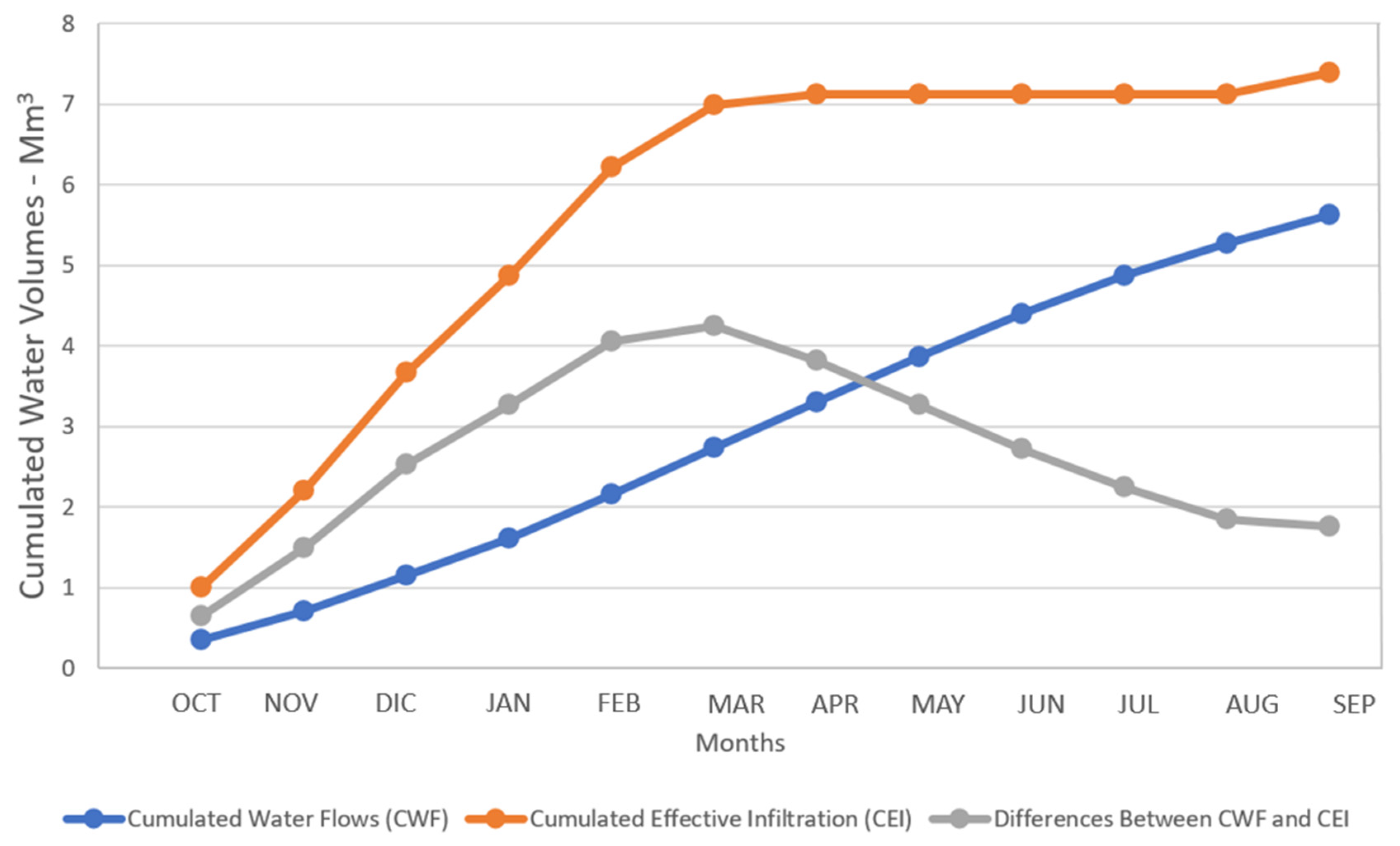
Table 4 and Figure 7 show the values of the monthly average flow rates of (1) the Santissima aqueduct, (2) the effective infiltration (i.e., groundwater recharge), (3) the rainfall, (4) the cumulative conveyed volumes, (5) effective infiltration volumes, (6) and the differences between the last two. Figure 8 shows the values of cumulative rainfall and cumulative conveyed water flows and their monthly differences.
The results reveal that the annual average potential recharge, or effective infiltration, is about 7.384 Mm3, corresponding to 234.15 L/s potentially available to supply the Santissima aqueduct. As expected, the average recharge decreases significantly from May to August, due to the scarce rain and the considerable evapotranspiration in summer, nonetheless, the rainy season from September to March/April ensures the replenishment of the aquifer over the hydrological year. In volumetric terms (see Figure 8), the total balance at the end of the hydrological year, corresponding to the difference between the average annual recharge and the water conveyed in the aqueduct, is about 1.750 Mm3, about 23.7% of the calculated average annual recharge. It should be stressed that the water balance only considers the flows conveyed in the aqueduct, thus disregarding discharges of disconnected springs, such as the ones drained in the Carbonara Gallery, whose average flow rate of 22.72 L/s (see Table 1) corresponds to 0.716 Mm3/year. Including this further volume in the water balance would lead to a closure error of about 14%, very close to the theoretical threshold of 10%, usually considered when the inverse hydrogeological balance technique is applied [45].
4. Discussion
In this paper, an inverse GIS-based hydrogeological balance technique was applied to assess the monthly average potential recharge of the groundwater system also supplying the Santissima aqueduct.
Approaches based on the water balance computation for regional recharge assessment have been widely applied in literature due to their flexibility and the low data requirement for model calibration.
The major limitation of these approaches is that the accuracy of the recharge estimate depends on the accuracy of the measurements or estimates of the other components in the water balance equation. This limitation is critical when the magnitude of the recharge rate is small relative to that of the other variables (e.g., ET), such that small inaccuracies in values of those variables commonly result in large uncertainties in the recharge rate. For this reason, this kind of approach is not suitable for ungauged basins in arid environments, where the water balance is almost negative throughout the year [9,10,46,47]. However, calculation of the water balance on a daily time step can help to solve this issue, as P sometimes greatly exceeds ET on a single day, even in arid regions [13,48,49].
In temperate and humid zones, as is the case considered in the present study, inaccuracies in the water-balance determination are normally sufficiently small, in comparison with the magnitude of the recharge component, to allow for a reasonable estimate. Therefore, averaging over longer periods (e.g., months) is not an issue, since recharge processes are not related to extreme precipitation events only.
The embedding of the methodology within a geographical information system for data acquisition and processing allows for a regional analysis of recharge and could be used to evaluate the effects of land cover changes on recharge, thus contributing to improving groundwater protection and sustainable use.
As highlighted by many authors [50,51,52], hydrogeological modeling using GIS has become a standard for environmental studies and allows for the integration of different spatial variable physiographic datasets (i.e., land cover, geological, morphologic, climatic), largely available in digital format.
On the other hand, some limitations can derive from the low resolution of some physiographic layers. For instance, in our case study, the resolution of the hydrogeological map is too coarse to provide a detailed delineation of the sub-hydro-structures and a proper geological characterization, which could help in reducing the area of investigation and to better select the potential infiltration coefficient for each hydrogeological unit.
Conversely, from the original method, in this study we used the Budyko formulation to estimate ET at the monthly scale, retrieving monthly potential evapotranspiration values from the Global Aridity Index and Potential Evapotranspiration Climate Database v2.
These days, potential evapotranspiration formulas exist in abundance, reflecting the difficulty of conceptualizing this process into a simple expression [53]. This issue has also been investigated concerning uncertainty in hydrological modeling [54].
The diversity of mathematical formulations for evapotranspiration assessment, the data information needed, and the level of required expertise make it difficult to select the most appropriate formula for a given situation. Consequently, different approaches are often analyzed and compared for specific areas, as illustrated by [55,56,57,58,59,60,61].
The Budyko model has long been considered a useful tool to investigate the catchment-scale interactions between hydroclimatic variables and catchment characteristics [62,63,64]. Numerous efforts were directed to extend the applicability of the Budyko model from the originally designed long-term mean-annual perspective to the shorter temporal scales such as annual [65,66,67,68], seasonal [69], and monthly time scales [36,70].
At the annual and monthly scales, the performance of the Budyko framework to assess the catchment scale water balance has been generally proven to be more accurate in arid climates than in humid climates [71], likely due to more complex interactions between the climate factors and catchment properties, such as vegetation and topography.
Under arid climates, the partitioning of precipitation P into evapotranspiration ET, infiltration I, and runoff R, is mainly controlled by P [36,72]; however, water storage changes can also have a significant or even predominant impacts on the intra-annual and interannual variability of ET [71].
Recently, the authors of [73] investigated the role of climatic factors and catchment responses in the errors of the Budyko framework annual and monthly predicted evaporation, E, through a decomposition framework of the error variance and covariance terms of precipitation, potential evapotranspiration, runoff, and water storage change. By applying this methodology to 14 major river basins in China with different climatic conditions, they found that these terms play a comparable role in the errors of the predicted evaporation under humid conditions, whereas the water storage change plays a dominant role in the prediction errors in arid climates. This finding suggests that incorporating catchment properties in the Budyko framework is not relevant in improving the ET predictions in humid regions, unlike arid ones.
For the considered case-study area, the application of the Budyko formulation for evapotranspiration assessment has given satisfactory results, in agreement with a previous study applied to a case study area with similar climate conditions and complex topography [38]. Despite the non-closure error in the water balance, likely resulting from a partial knowledge of spring discharges, the application of the Budyko framework allows for the strong effect of seasonal variability to be considered in the water balance at the intra-annual scale. In particular, it can contribute to reducing the uncertainty in recharge estimates during the dry seasons, when the climate of the area turns to semiarid even at the highest elevations.
5. Conclusions
A modified GIS-based inverse hydrogeological balance technique has been applied to assess the monthly and annual average potential recharge of a sub hydro structure of the eastern Peloritani water body (northeastern Sicily). The Budyko formulation has been applied to assess the evapotranspiration component in the water balance equation.
The proposed simple approach provides a preliminary, although reasonable, estimation of the potential aquifer recharge, roughly representing the amount of available water for water supply, in an ungauged hydrogeological basin.
The methodology represents a valid alternative when the lack of direct measurements of the surface and groundwater flow rates prevents the use of complex numerical modeling.
The application of the methodology to a humid region allows for the use of the monthly scale instead of the daily time scale, commonly used in water balance computations in arid and semiarid regions to reduce uncertainties in the estimates. The estimates of aquifer recharge on a monthly scale can be used to support rational and sustainable water resources management.
Current estimates of potential recharge can be used in the future for several hydrogeological applications, such as validating the conceptual model of groundwater flow and groundwater recharge area delineation and supporting the assessment of groundwater vulnerability to pollution.
Further improvements of the methodology can be obtained by a more detailed geological and hydrogeological knowledge of the area, which is needed to better delineate the hydrogeological basins. To this end, it is worth emphasizing that the estimation of groundwater recharge is an iterative process, involving progressive aquifer-response data collection to realistically determine recharge processes. The combination of field measurements, remote sensing, and GIS technology could lead to a better understanding and quantification of recharge over large areas.
Further studies are ongoing to evaluate the mean monthly regional water balance by using a long-term monthly global dataset, combining multiple data sources, and making a comparison with the results achieved in the current study. Also, other measurement campaigns are planned to acquire further knowledge on the case study area.
Author Contributions
Conceptualization and methodology, I.B. and B.B.; data curation, formal analysis, and validation, I.B.; writing—original draft preparation, I.B.; writing—review and editing, B.B.; visualization, I.B.; supervision, B.B. All authors have read and agreed to the published version of the manuscript.
Funding
This research was funded by AMAM S.p.A. within the research agreement with the Department of Engineering of the University of Messina “Attività di studio e ricerca per la redazione di studi idrologici a supporto dell’istanza di rinnovo della concessione delle derivazioni di acque dal sistema di pozzi e gallerie Bufardo-Torrerossa e della domanda per l’utilizzo delle acque sorgentizie che alimentano l’acquedotto della Santissima del Comune di Messina”. Agreement No. 45357, 19 June 2017 (in Italian).
Institutional Review Board Statement
Not applicable.
Informed Consent Statement
Not applicable.
Data Availability Statement
Rainfall data were taken from the Basin Authority of the Hydrographic District of Sicily website (https://www.regione.sicilia.it/istituzioni/regione/strutture-regionali/presidenza-regione/autorita-bacino-distretto-idrografico-sicilia/annali-idrologici, access date: 13 December 2021); aridity index values were taken from the Global Aridity Index and Potential Evapotranspiration Climate Database v2 (https://figshare.com/articles/Global_Aridity_Index_and_Potential_Evapotranspiration_ET0_Climate_Database_v2/7504448/3, access date: 13 December 2021); the flow rate information in Table 1 was provided by AMAM S.p.A. through personal communication.
Acknowledgments
The authors would like to acknowledge Alfredo Natoli for his fundamental help in the identification of the groundwater body and Giuseppe Tito Aronica for his valuable comments on the model development.
Conflicts of Interest
The authors declare no conflict of interest.
References
- Stoll, S.; Franssen, H.J.H.; Barthel, R.; Kinzelbach, W. What can we learn from long-term groundwater data to improve climate change impact studies? Hydrol. Earth Syst. Sci. 2011, 15, 3861–3875. [Google Scholar] [CrossRef] [Green Version]
- Liu, H. Impact of climate change on groundwater recharge in dry areas: An ecohydrology approach. J. Hydrol. 2011, 407, 175–183. [Google Scholar] [CrossRef]
- Taylor, R.G.; Scanlon, B.; Döll, P.; Rodell, M.; van Beek, R.; Wada, Y.; Longuevergne, L.; Leblanc, M.; Famiglietti, J.S.; Edmunds, M.; et al. Ground water and climate change. Nat. Clim. Chang. 2013, 3, 322–329. [Google Scholar] [CrossRef] [Green Version]
- Döll, P. Vulnerability to the impact of climate change on renewable groundwater resources: A global-scale assessment. Environ. Res. Lett. 2009, 4, 035006. [Google Scholar] [CrossRef]
- Taylor, R.G.; Todd, M.C.; Kongola, L.; Maurice, L.; Nahozya, E.; Sanga, H.; MacDonald, A.M. Evidence of the dependence of groundwater resources on extreme rainfall in East Africa. Nat. Clim. Chang. 2013, 3, 374–378. [Google Scholar] [CrossRef] [Green Version]
- Healy, R.W.; Cook, P.G. Using groundwater levels to estimate recharge. Hydrogeol. J. 2002, 10, 91–109. [Google Scholar] [CrossRef]
- Moeck, C.; von Freyberg, J.; Schirmer, M. Groundwater recharge predictions in contrasted climate: The effect of model complexity and calibration period on recharge rates. Environ. Model. Softw. 2018, 103, 74–89. [Google Scholar] [CrossRef]
- Von Freyberg, J.; Moeck, C.; Schirmer, M. Estimation of groundwater recharge and drought severity with varying model complexity. J. Hydrol. 2015, 527, 844–857. [Google Scholar] [CrossRef]
- Lerner, D.N.; Issar, A.S.; Simmers, I. Groundwater Recharge. A Guide to Understanding and Estimating Natural Recharge; IAH International Contributions to Hydrogeology: Hannover, Germany, 1990; p. 345. [Google Scholar]
- De Vries, J.J.; Simmers, I. Groundwater recharge: An overview of processes and challenges. Hydrogeol. J. 2002, 10, 5–17. [Google Scholar] [CrossRef]
- Scanlon, B.R.; Healy, R.W.; Cook, P. Choosing Appropriate Techniques for Quantifying Groundwater Recharge. Hydrogeol. J. 2002, 10, 18–39. [Google Scholar] [CrossRef]
- Smerdon, B.D.; Drewes, J.E. Groundwater recharge: The intersection between humanity and hydrogeology. J. Hydrol. 2017, 555, 909–911. [Google Scholar] [CrossRef]
- Carletti, A.; Canu, S.; Motroni, A.; Ghiglieri, G. A combined methodology for estimating the potential natural aquifer recharge in an arid environment. Hydrol. Sci. J. 2019, 64, 1727–1745. [Google Scholar] [CrossRef]
- Moeck, C.; Grech-Cumbo, N.; Podgorski, J.; Bretzler, A.; Gurdak, J.J.; Berg, M.; Schirmer, M. A global-scale dataset of direct natural groundwater recharge rates: A review of variables, processes and relationships. Sci. Total. Environ. 2020, 717, 137042, ISSN 0048-9697. [Google Scholar] [CrossRef]
- Jakeman, A.J.; Post, D.A.; Beck, M.B. From data and theory to environmental model: The case of rainfall-runoff. Environmetrics 1994, 5, 297–314. [Google Scholar] [CrossRef]
- Ivkovic, K.M.; Letcher, R.A.; Croke, B.F.W. Use of a simple surface-groundwater interaction model to inform water management. Aust. J. Earth Sci. 2009, 56, 61–70. [Google Scholar] [CrossRef]
- Croke, B.F.W.; Smith, A.B.; Jakeman, A.J. A One-Parameter Groundwater Discharge Model Linked to the IHACRES Rainfall-Runo_ Model. In Proceedings of the 1st International Congress on Environmental Modelling and Software, Lugano, Switzerland, 24–27 June 2002. [Google Scholar]
- Borzì, I.; Bonaccorso, B.; Fiori, A. A Modified IHACRES Rainfall-Runoff Model for Predicting the Hydrologic Response of a River Basin Connected with a Deep Groundwater Aquifer. Water 2019, 11, 2031. [Google Scholar] [CrossRef] [Green Version]
- Sophocleous, M.; Perkins, S.P. Methodology and application of combined watershed and ground-water models in Kansas. J. Hydrol. 2000, 236, 185–201. [Google Scholar] [CrossRef]
- Harbaugh, A.W. MODFLOW-2005, the U.S. Geological Survey Modular Ground-Water Model—The Ground-Water Flow Process: U.S. Geological Survey Techniques and Methods 6-A16; U.S. Department of the Interior: Washington, DC, USA; U.S. Geological Survey: Reston, VA, USA, 2005. [Google Scholar]
- Mohammadi, K. Groundwater Table Estimation Using MODFLOW and Artificial Neural Networks. In Practical Hydroinformatics: Water Science and Technology Library; Abrahart, R.J., See, L.M., Solomatine, D.P., Eds.; Springer: Berlin/Heidelberg, Germany, 2009; Volume 68. [Google Scholar] [CrossRef]
- Brunner, P.; Doherty, J.; Simmons, C.T. Uncertainty assessment and implications for data acquisition in support of integrated hydrologic models. Water Resour. Res. 2012, 48, W07513. [Google Scholar] [CrossRef] [Green Version]
- Friedel, M.J. Coupled inverse modeling of vadose zone water, heat, and solute transport: Calibration constraints, parameter nonuniqueness, and predictive uncertainty. J. Hydrol. 2005, 312, 148–175. [Google Scholar] [CrossRef]
- Hartmann, A.; Gleeson, T.; Wada, Y.; Wagener, T. Enhanced groundwater recharge rates and altered recharge sensitivity to climate variability through subsurface heterogeneity. Proc. Natl. Acad. Sci. USA 2017, 114, 2842–2847. [Google Scholar] [CrossRef] [PubMed] [Green Version]
- Ines, A.V.; Droogers, P. Inverse modelling in estimating soil hydraulic functions: A genetic algorithm approach. Hydrol. Earth Syst. Sci. Discuss. 2002, 6, 49–66. [Google Scholar] [CrossRef] [Green Version]
- Moeck, C.; Brunner, P.; Hunkeler, D. The influence ofmodel structure on groundwater recharge rates in climate-change impact studies. Hydrogeol. J. 2016, 24, 1171–1184. [Google Scholar] [CrossRef] [Green Version]
- Shoeller, H. Les Eaux Souterraines; Masson: Paris, France, 1962. (In French) [Google Scholar]
- Civita MCivita, M.; Manzone, L.; Olivero, G.; Vigna, B. Le sorgenti del Maira. Studio di una risorsa idrica di importanza strategica [The Maira Springs. Study of a strategic water resource]. In Atti 2 Conv. Naz. “Protezione e Gestione delle Acque Sotterranee: Metodologie, Tecnologie e Obiettivi”; Nonatola: Modena, Italy, 1995; Volume 1, pp. 231–238. [Google Scholar]
- Civita, M.; De Maio, M. SINTACS Un sistema parametrico per la valutazione e la cartografia della vulnerabilità degli acquiferi all’inquinamento. In Metodologia e Automazione; Pitagora Editrice: Bologna, Italy, 1997; p. 191. (In Italian) [Google Scholar]
- Civita, M.; De Maio, M. Average groundwater recharge in carbonate aquifers: A GIS processed numerical model. In Proceedings of the 7th Conference on Limestone Hydrology and Fissured Media, Besançon, France, 20–23 September 2001; pp. 93–100. [Google Scholar]
- Koutsoyiannis, D. Seeking Parsimony in Hydrology and Water Resources Technology, European Geosciences Union General Assembly 2009, Geophysical Research Abstracts; European Geosciences Union: Munich, Germany, 2009; Volume 11. [Google Scholar] [CrossRef]
- Budyko, M.I. Climate and Life; Academic: San Diego, CA, USA, 1974; p. 508. [Google Scholar]
- Turc, L. Calcul du bilan de l’eau: Evaluation en function des precipitation et des temperatures. IAHS Publ. 1954, 37, 88–200. (In French) [Google Scholar]
- Zhang, L.; Potter, N.; Hickel, K.; Zhang, Y.; Shao, Q. Water balance modeling over variable time scales based on the Budyko framework—Model development and testing. J. Hydrol. 2008, 360, 117–131. [Google Scholar] [CrossRef]
- Ferrara, V. The optimal management of groundwater resources in the Peloritani Mountains area (North-East-Sicily). In Proceedings of the International Conference on Water Resources in Mountain Regions, Lausanne, Switzerland, 27 August–1 September 1990. [Google Scholar]
- Ferrara, V. Vulnerabilità All’inquinamento degli Acquiferi dell’Area Peloritani Sicilia Nord-Orientale. Quaderni di Tecniche di Protezione Ambientale, 66; Pitagora Editrice: Bologna, Italy, 1990. (In Italian) [Google Scholar]
- Regione Siciliana. Piano di Gestione del Distretto Idrografioco della Sicilia; PGDI: Regione Sicilia, Italy, 2016. (In Italian) [Google Scholar]
- Borzì, I.; Bonaccorso, B.; Aronica, G.T. The Role of DEM Resolution and Evapotranspiration Assessment in Modeling Groundwater Resources Estimation: A Case Study in Sicily. Water 2020, 12, 2980. [Google Scholar] [CrossRef]
- Civita, M. Idrogeologia Applicata e Ambientale; CEA Editore: Roma, Italy, 2005; ISBN 978-8808087416. (In Italian) [Google Scholar]
- Blöschl, G.; Sivapalan, M.; Wagener, T.; Viglione, A.; Savenije, H. Runoff Prediction in Ungauged Basins: Synthesis across Processes, Places and Scales; Cambridge University Press: Cambridge, UK, 2013. [Google Scholar]
- Thornthwaite, C.W. An approach toward a rational classification of climate. Geogr. Rev. 1948, 38, 55–94. [Google Scholar] [CrossRef]
- Penman, H.L. 1948 Natural evaporation from open water, bare soil and grass. Proc. R. Soc. A Math. Phys. Eng. Sci. 1948, 193, 120–145. [Google Scholar] [CrossRef] [Green Version]
- Trabucco, A.; Zomer, R.J. Global Aridity Index and Potential Evapo-Transpiration (ET0) Climate Database v2. CGIAR Consortium for Spatial Information (CGIAR-CSI). Published online, available from the CGIAR-CSI GeoPortal. 2018. Available online: https://cgiarcsi.community (accessed on 13 December 2021).
- Doherty, J.E.; Hunt, R.J. Approaches to Highly Parameterized Inversion: A Guide to Using PEST for Groundwater-Model Calibration; US Geological Survey: Reston, VA, USA; US Department of the Interior: Washington, DC, USA, 2010. [Google Scholar]
- Condon, L.E.; Maxwell, R.M. Simulating the sensitivity of evapotranspiration and streamflow to large-scale groundwater depletion. Sci. Adv. 2019, 5, eaav4574. [Google Scholar] [CrossRef] [PubMed] [Green Version]
- Gee, G.W.; Hillel, D. Groundwater recharge in arid regions: Review and critique of estimation methods. Hydrol. Process 1988, 2, 255–266. [Google Scholar] [CrossRef]
- Hendrickx, J.M.H.; Walker, G.R. Recharge from precipitation. In Recharge of Phreatic Aquifers in (Semi-)Arid Areas; Simmers, I., Ed.; IAH International Contributions to Hydrogeoleology 19; A.A. Balkema: Rotterdam, The Netherlands, 1997; pp. 19–111. [Google Scholar]
- Carrera-Hernández, J.J.; Gaskin, S.J. Spatio temporal analysis of daily precipitation and temperature in the Basin of Mexico. J. Hydrol. 2007, 336, 231–249. [Google Scholar] [CrossRef]
- Ghiglieri, G.; Carletti, A.; Pittalis, D. Runoff coefficient and average yearly natural aquifer recharge assessment by physiography-based indirect methods for the island of Sardinia (Italy) and its NW area (Nurra). J. Hydrol. 2014, 519, 1779–1791. [Google Scholar] [CrossRef]
- Shaban, A.; Khawlie, M.; Abdallah, C. Use of remote sensing and GIS to determine recharge potential zones: The case of Occidental Lebanon. Hydrogeol. J. 2006, 14, 433–443. [Google Scholar] [CrossRef]
- Storck, P.; Bowling, L.; Wetherbee, P.; Lettenmaier, D. Application of a GISbased distributed hydrology model for prediction of forest harvest effects on peak stream flow in the Pacific Northwest. Hydrol. Process. 1998, 12, 889–904. [Google Scholar] [CrossRef]
- Vijay, R.; Panchbhai, N.; Gupta, A. Spatio-temporal analysis of groundwater recharge and mound dynamics in an unconfined aquifer: A GIS-based approach. Hydrol. Process. 2007, 21, 2760–2764. [Google Scholar] [CrossRef]
- Seiller, G.; Anctil, F.J. How do potential evapotranspiration formulas influence hydrological projections? Hydrol. Sci. J. 2016, 61, 2249–2266. [Google Scholar] [CrossRef] [Green Version]
- Hulme, M.; Carter, T.R.; Viner, D. Representing Uncertainty in Climate Change Scenarios and Impact Studies: ECLAT-2 Workshop Report no. 1; Climatic Research Unit: Norwich, UK, 1999. [Google Scholar]
- Verstraeten, W.W.; Veroustraete, F.; Feyen, J. Assessment of evapotranspiration and soil moisture content across different scales of observation. Sensors 2008, 8, 70–117. [Google Scholar] [CrossRef] [Green Version]
- Brutsaert, W. Evaporation into the Atmosphere: Theory, History and Applications; Springer: Dordrecht, The Netherlands, 1982. [Google Scholar]
- Singh, V.P. Hydrologic Systems: Watershed Modeling; Prentice Hall: Englewood Cliffs, NJ, USA, 1989; Volume 2. [Google Scholar]
- Jensen, M.E.; Burman, R.D.; Allen, R.G. Evapotranspiration and Irrigation Water Requirements; American Society of Civil Engineers: Reston, VA, USA, 1990. [Google Scholar]
- Morton, F.I. Evaporation research—A critical review and its lessons for the environmental sciences. Crit. Rev. Environ. Sci. Technol. 1994, 24, 237–280. [Google Scholar] [CrossRef]
- Singh, V.P.; Xu, C.-Y. Evaluation and generalization of 13 mass transfer equations for determining free water evaporation. Hydrol. Process. 1997, 11, 311–323. [Google Scholar] [CrossRef]
- Donohue, R.J.; McVicar, T.R.; Roderick, M.L. Assessing the ability of potential evaporation formulations to capture the dynamics in evaporative demand within a changing climate. J. Hydrol. 2010, 386, 186–197. [Google Scholar] [CrossRef]
- Donohue, R.J.; Roderick, M.L.; McVicar, T.R. On the importance of including vegetation dynamics in Budyko’s hydrological model. Hydrol. Earth Syst. Sci. 2007, 11, 983–995. [Google Scholar] [CrossRef] [Green Version]
- Donohue, R.J.; Roderick, M.L.; McVicar, T.R. Can dynamic vegetation information improve the accuracy of Budyko’s hydrological model? J. Hydrol. 2010, 390, 23–34. [Google Scholar] [CrossRef]
- Donohue, R.J.; Roderick, M.L.; McVicar, T.R. Assessing the differences in sensitivities of runoff to changes in climatic conditions across a large basin. J. Hydrol. 2011, 406, 234–244. [Google Scholar] [CrossRef]
- Koster, R.D.; Suarez, M.J. A simple framework for examining the interannual variability of land surface moisture fluxes. J. Climate 1999, 12, 1911–1917. [Google Scholar] [CrossRef]
- Sankarasubramanian, A.; Vogel, R.M. Annual hydroclimatology of the United States. Water Resour. Res. 2002, 38, 1083. [Google Scholar] [CrossRef]
- Potter, N.J.; Zhang, L. Interannual variability of catchment water balance in Australia. J. Hydrol. 2009, 369, 120–129. [Google Scholar] [CrossRef]
- Wang, T.; Sun, F.; Lim, W.H.; Wang, H.; Liu, W.; Liu, C. The Predictability of annual evapotranspiration and runoff in humid and nonhumid catchments over China: Comparison and quantification. J. Hydrometeor. 2018, 19, 533–545. [Google Scholar] [CrossRef]
- Chen, X.; Alimohammadi, N.; Wang, D. Modeling interannual variability of seasonal evaporation and storage change based on the extended Budyko framework. Water Resour. Res. 2013, 49, 6067–6078. [Google Scholar] [CrossRef] [Green Version]
- Tekleab, S.; Uhlenbrook, S.; Mohamed, Y.; Savenije, H.H.G.; Temesgen, M.; Wenninger, J. Water balance modeling of Upper Blue Nile catchments using a top-down approach. Hydrol. Earth Syst. Sci. 2011, 15, 2179–2193. [Google Scholar] [CrossRef] [Green Version]
- Wu, C.H.; Yeh, P.J.-F.; Wu, H.C.; Hu, B.X.; Huang, G.R. Global analysis of the role of terrestrial water storage in the evapotranspiration estimated from the Budyko framework at the annual-to-monthly timescales. J. Hydrometeorol. 2019, 20, 2003–2021. [Google Scholar] [CrossRef]
- Zhang, L.; Hickel, K.; Dawes, W.R.; Chiew, F.H.S.; Western, A.W.; Briggs, P.R. A rational function approach for estimating mean annual evaporation. Water Resour. Res. 2004, 40, W02502. [Google Scholar] [CrossRef]
- Wu, C.H.; Yeh, P.J.-F.; Hu, B.X.; Huang, G.R. Controlling factors of errors in the predicted annual and monthly evaporation from the Budyko framework. Adv. Water Resour. 2018, 121, 432–445. [Google Scholar] [CrossRef]
Figure 1.
On the left-hand side, the eastern Peloritani study area with its topography, the corresponding river basins, the location of the springs feeding the Santissima aqueduct, and the weather stations. On the right-hand side, the geographical location of the case study area at the national scale (projected coordinate system: UTM WGS 1984; Zone 33N).

Figure 2.
Mean monthly temperature in the case study area.

Figure 3.
Interannual variability of annual precipitation and mean annual temperature.

Figure 4.
Main hydrogeological formations of the case study area (excerpted from the regional map of groundwater bodies included in the Management Plan of the hydrographic district of Sicily, Tav. B1 [37]; (projected coordinate system: UTM WGS 1984; Zone 33N).
Figure 4.
Main hydrogeological formations of the case study area (excerpted from the regional map of groundwater bodies included in the Management Plan of the hydrographic district of Sicily, Tav. B1 [37]; (projected coordinate system: UTM WGS 1984; Zone 33N).

Figure 5.
Flowchart of the methodology.

Figure 6.
Linear regression of mean monthly precipitation values versus station elevations.

Figure 7.
Main components of the hydrogeological water balance of the groundwater body supplying the Santissima aqueduct along the hydrological year.
Figure 7.
Main components of the hydrogeological water balance of the groundwater body supplying the Santissima aqueduct along the hydrological year.

Figure 8.
Cumulative effective infiltration volumes, cumulative conveyed water volumes, and corresponding deviation between the two volumes.
Figure 8.
Cumulative effective infiltration volumes, cumulative conveyed water volumes, and corresponding deviation between the two volumes.


Table 1.
Measured and average flow rates (L/s) for each spring group connected with the aqueduct.
| Spring Group | Flow Rate in Mid-July 2018 (L/s) | Flow Rate in Mid-February 2019 (L/s) | Average Flow Rate (L/s) |
|---|---|---|---|
| Bocche d’Acqua | 34.00 | 69.06 | 51.53 |
| Bottino | 5.80 | 11.76 | 8.78 |
| Cianciana | 6.70 | 13.58 | 10.14 |
| Sciara Cambria | 2.74 | 5.55 | 4.14 |
| Faraone-Larioti | 2.80 | 5.64 | 4.22 |
| Femminamorta | 2.20 | 4.45 | 3.32 |
| Scacciafica | 0.97 | 1.96 | 1.46 |
| Cammarone | 0.16 | 0.32 | 0.24 |
| Ula Pernice | 0.41 | 0.84 | 0.62 |
| Ilici Lunga–Cannizzola | 6.34 | 12.86 | 9.60 |
| Pomara–Bertuccio | 2.56 | 5.20 | 3.88 |
| Porta | 2.96 | 6.14 | 4.55 |
| Santissima | 36.1 | 73.25 | 54.67 |
| Corvo Nociara | 1.98 | 4.03 | 3.01 |
| Griole-Iaddizzi | 1.39 | 3.20 | 2.29 |
| Grillo | 2.53 | 5.12 | 3.82 |
| Carbonara Gallery (out of order) | 15.00 | 30.45 | 22.72 |
Table 2.
Mean monthly and annual rainfall values (in mm) in each station for the period 2003–2019.
| Station Code | Elevation (m a.s.l.) | Jan. | Feb. | Mar. | Apr. | May. | Jun. | Jul. | Aug. | Sep. | Oct. | Nov. | Dec. | Mean |
|---|---|---|---|---|---|---|---|---|---|---|---|---|---|---|
| Fiumedinisi (248) | 440.00 | 130.33 | 122.00 | 121.04 | 71.95 | 28.55 | 23.29 | 12.56 | 26.59 | 126.27 | 164.39 | 157.22 | 160.81 | 95.42 |
| Messina (251) | 420.00 | 123.08 | 108.37 | 110.75 | 55.62 | 38.73 | 37.98 | 14.27 | 27.62 | 88.20 | 114.64 | 140.90 | 141.18 | 83.44 |
| S Pier Niceto (249) | 460.00 | 98.17 | 94.32 | 83.46 | 56.28 | 29.69 | 27.01 | 10.56 | 30.86 | 84.43 | 94.00 | 118.40 | 116.88 | 70.34 |
| Torregrotta (261) | 26.00 | 120.65 | 116.05 | 93.08 | 62.75 | 29.92 | 23.19 | 7.35 | 35.52 | 73.58 | 95.64 | 102.46 | 131.40 | 74.30 |
| Antillo (313) | 796.00 | 185.37 | 202.58 | 161.59 | 66.44 | 28.19 | 22.44 | 12.03 | 22.63 | 121.16 | 209.54 | 233.39 | 183.66 | 120.75 |
Table 3.
Mean monthly values (Mm3/month) of the components of the hydrogeological balance.
| Variable | Jan. | Feb. | Mar. | Apr. | May. | Jun. | Jul. | Aug. | Sep. | Oct. | Nov. | Dec. |
|---|---|---|---|---|---|---|---|---|---|---|---|---|
| Rainfall | 2.010 | 2.184 | 1.640 | 0.778 | 0.317 | 0.226 | 0.100 | 0.338 | 1.161 | 2.003 | 2.198 | 2.197 |
| Evapotranspiration | 0.551 | 0.600 | 0.714 | 0.618 | 0.316 | 0.226 | 0.100 | 0.337 | 0.852 | 0.819 | 0.644 | 0.460 |
| Effective rainfall | 1.459 | 1.584 | 0.926 | 0.160 | 0.002 | 0.000 | 0.000 | 0.001 | 0.309 | 1.184 | 1.554 | 1.737 |
| Infiltration rate | 1.240 | 1.347 | 0.787 | 0.136 | 0.001 | 0.000 | 0.000 | 0.000 | 0.263 | 1.006 | 1.321 | 1.476 |
Table 4.
Mean monthly values of the main components of the Santissima system for the hydrological year.
Table 4.
Mean monthly values of the main components of the Santissima system for the hydrological year.
| Month | Conveyed Flows (L/s) (1) | Effective Infiltration (EI) (L/s) (2) | Rainfall (L/s) (3) | Cumulative Conveyed Volumes (Mm3) (4) | Cumulative EI Volumes (Mm3) (5) | Differences between (5) and (4) (Mm3) (6) |
|---|---|---|---|---|---|---|
| October | 132.356 | 375.621 | 747.785 | 0.355 | 1.006 | 0.652 |
| November | 147.438 | 493.236 | 820.559 | 0.711 | 2.199 | 1.488 |
| December | 161.544 | 551.165 | 820.114 | 1.144 | 3.676 | 2.532 |
| January | 177.186 | 462.877 | 750.312 | 1.603 | 4.875 | 3.272 |
| February | 207.863 | 502.741 | 815.555 | 2.160 | 6.222 | 4.062 |
| March | 221.922 | 293.933 | 612.230 | 2.735 | 6.984 | 4.249 |
| April | 209.500 | 50.684 | 290.352 | 3.296 | 7.119 | 3.823 |
| May | 209.533 | 0.498 | 118.412 | 3.857 | 7.121 | 3.263 |
| June | 208.711 | 0.023 | 84.475 | 4.398 | 7.121 | 2.722 |
| July | 178.444 | 0.000 | 37.462 | 4.876 | 7.121 | 2.245 |
| August | 151.467 | 0.173 | 126.063 | 5.269 | 7.121 | 1.852 |
| September | 136.267 | 98.183 | 433.651 | 5.634 | 7.384 | 1.750 |
Publisher’s Note: MDPI stays neutral with regard to jurisdictional claims in published maps and institutional affiliations. |
© 2021 by the authors. Licensee MDPI, Basel, Switzerland. This article is an open access article distributed under the terms and conditions of the Creative Commons Attribution (CC BY) license (https://creativecommons.org/licenses/by/4.0/).
Share and Cite
MDPI and ACS Style
Borzì, I.; Bonaccorso, B. Quantifying Groundwater Resources for Municipal Water Use in a Data-Scarce Region. Hydrology 2021, 8, 184. https://0-doi-org.brum.beds.ac.uk/10.3390/hydrology8040184
AMA Style
Borzì I, Bonaccorso B. Quantifying Groundwater Resources for Municipal Water Use in a Data-Scarce Region. Hydrology. 2021; 8(4):184. https://0-doi-org.brum.beds.ac.uk/10.3390/hydrology8040184
Chicago/Turabian StyleBorzì, Iolanda, and Brunella Bonaccorso. 2021. "Quantifying Groundwater Resources for Municipal Water Use in a Data-Scarce Region" Hydrology 8, no. 4: 184. https://0-doi-org.brum.beds.ac.uk/10.3390/hydrology8040184
Note that from the first issue of 2016, this journal uses article numbers instead of page numbers. See further details here.