Perspective Impact on Water Environment and Hydrological Regime Owing to Climate Change: A Review

Abstract

This study summarizes reviews on climate change’s impact on the water environment and hydrological regime. The results indicate a strong relationship between the climatological parameters and hydrological patterns. This relationship can be determined in two steps: (1) define the variations in climatological factors, particularly temperature and precipitation, and (2) measure the variations in runoff and inflows to streams and river systems using different statistical and global climate modeling approaches. It is evident that the increasing global temperatures have significant positive effects on runoff variations and evapotranspiration. Similarly, the increase in temperature has speeded up the melting of glaciers and ice on hilly terrains. This is causing frequent flash floods and a gradual rise in the sea level. These factors have altered the timing of stream flow into rivers. Furthermore, the accumulation of greenhouse gases, variations in precipitation and runoff, and sea-level rise have significantly affected freshwater quality. These effects are likely to continue if timely mitigation and adaptation measures are not adopted.

1. Introduction

To make water reserves more sustainable, it is necessary to determine how water quantity and quality would vary. Simulated data from regional models are a standard tool for predicting future water resources. Uncertainty and variability across models typically hinder the downscaling of large-scale water supply system predictions to small watersheds for water resource management decisions [1,2]. There is certain unanimity in stream behavior in different regions [3,4,5]. However, this is not the case for watershed effects. According to Fatichi et al. [6], natural climate variation may be more critical for variations in stream flow than systematic variability. Land use and anthropogenic variables also play a role in sustainable water resource management [5,7,8,9,10]. The determination of the impact of climate on stream flows has been a challenge in previous regional research [11,12,13].

Climate change affects the hydrological cycle by affecting precipitation, evapotranspiration, and soil moisture. A World Metrological Organization (WMO) report (2021) indicated that the average global temperature has increased by 0.8 °C since 1880 (https://library.wmo.int/doc_num.php?explnum_id=11178; Accessed on 5 November 2022). In 2021, the average global temperature was around 1.11 ± 0.13 °C above the level of 1850–1900 but less warm than some recent years. However, additional precipitation is dispersed irregularly across the planet. Certain parts of the globe may experience significant reductions in precipitation or significant seasonal variations. Thus, research on the impacts of climate change on diverse hydrological components is vital [14,15,16]. Meko and Woodhouse (2005) observed the Sacramento and upper Colorado river basins [17]. They discovered that the seasonal flow from melting snow in the spring has decreased over time. Different studies confirmed this result by employing complicated statistical approaches and analyzing other basins [18,19,20].

Climate change alters the overall discharge regime of river basins and modifies the stream and base flow in channel systems. Establishing a multi-model set by considering multiple simulations through a series of global climate models (GCMs) has become a common approach for understanding climate disorders [21,22]. Arnell (1999) determined that climate change significantly impacts flood risk [23]. Previous studies have examined the flooding frequency over climate change using different projected climate scenarios [24,25]. However, the impact of climate change on hydrological regimes and river flows at the catchment scale is different from that at the regional scale [26,27,28].

Droughts and floods are observed to be a consequence of extraordinary spatial and temporal climate changes in Central America. This has been considered as a variability of climate “hot spots” [16,29,30]. It is critical to understand how climate change affects hydrological cycles and water resources. In this respect, four important drivers (Section 2) forcing climate change and the consequences on water resources have been discussed. This state-of-the-art review incorporates climate change’s impact on water resources and on hydrologic regimes (rainfall–runoff, river-flow system). In addition to the development of hydrological and climate models, downscaling strategies have been proposed to achieve geographical and temporal coverage for regional investigations of hydroclimatic change [30,31,32]. Fonseca and Santos [33] illustrated that to consider the uncertainties of future scenarios, it has become common practice to use climatic datasets produced by a multi-model group of regional climate models (RCMs) and forced by GCMs as inputs to run hydrological models (HMs). From the global scale to the local or basin scale, the chain “GCM–RCM–HM” is convenient for scenario-based information obtained by dynamic downscaling.

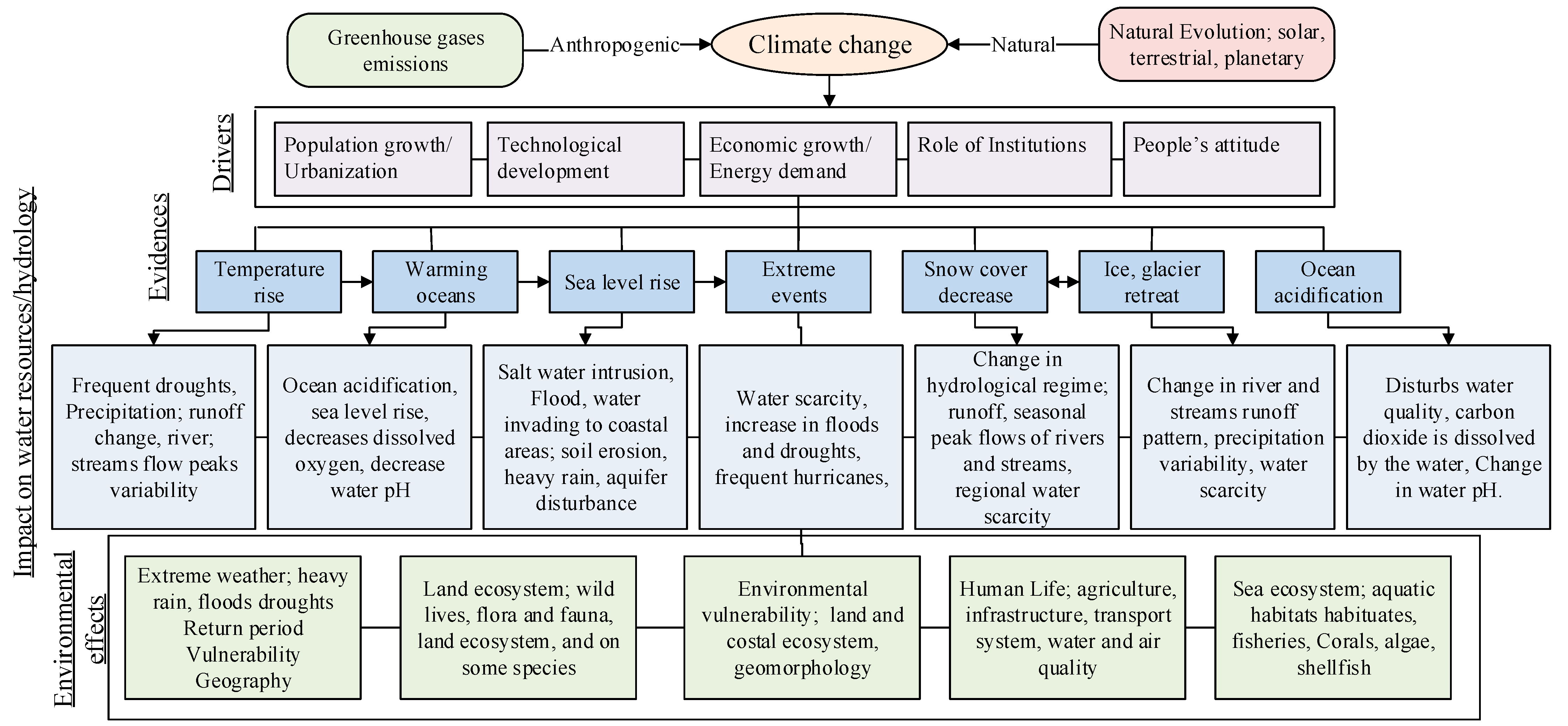
The objectives of this study are (1) to highlight the main driving forces behind climate change at a regional and global scale, (2) to describe the state-of-the-art methods to evaluate climate change and its impact on water and hydrologic regime, and (3) to describe the subsequent effects on water resources and the hydrological regime. A schematic design of the research is shown in Figure 1.

2. Driving Forces behind Climate Change

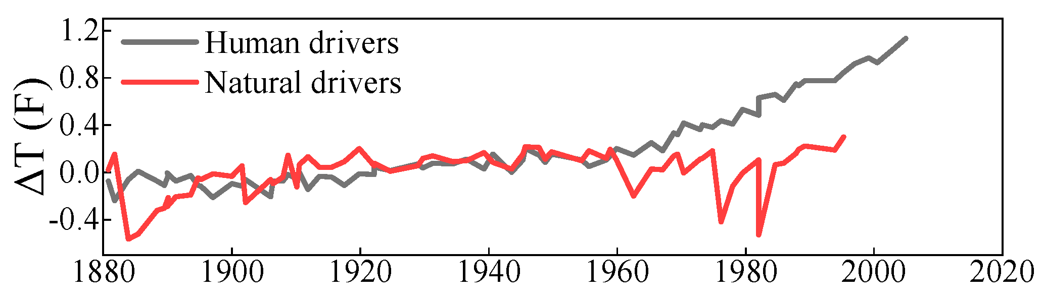
Climate change occurs through a complex set of interactive driving forces. According to the Intergovernmental Panel on Climate Change sixth assessment report (AR6; https://wg1.ipcc.ch/index.php/ar6/sixth-assessment-report-ar6; Accessed on 5 November 2022), human activity is the main driving force of climate change, whereas others contend that natural factors are also main causes. This ambiguity is due to inadequate data and methods to understand the phenomenon [34]. Both natural and human forces influence the Earth’s temperature, but the long-term trend observed over the last century can only be explained by the impact of human activities on the climate (Figure 2). Natural phenomena such as fluctuations in solar radiation and volcanic eruptions also have an impact on the Earth’s temperature. Similarly, Milankovitch cycles and El Niño Southern Oscillation (ENSO) are two other natural phenomena that are likely to change the Earth’s temperature. Milankovitch cycles occur as the Earth orbits the Sun, and its route and axis tilt might alter slightly. El Niño Southern Oscillation (ENSO) is a pattern of shifting Pacific Ocean water temperatures (https://www.metoffice.gov.uk/weather/climate-change/causes-of-climate-change; Accessed on 26 October 2022). However, they do not describe the warming we have experienced over the previous century. In this regard, the following four important human drivers are discussed in detail. These are also summarized in Table 1.

2.1. Population Growth

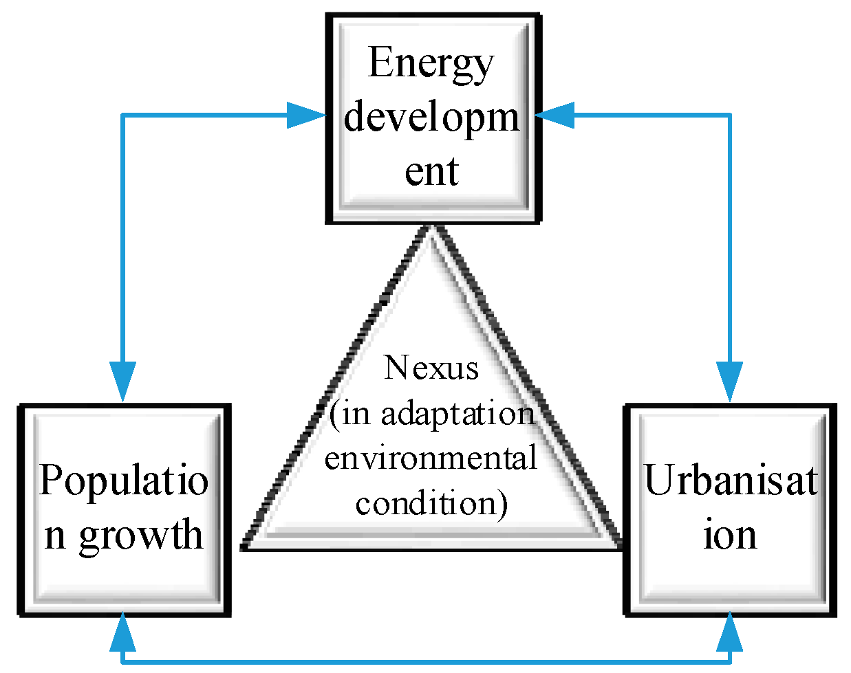
The human population increased from 1 billion to 7 billion in less than two centuries. Population growth has a direct relationship with the urbanization rate, and the growth of the urbanization rate in the past few decades is unprecedented. The two continents (Europe and Africa) are projected to be 56% and 64% urbanized, respectively, by the middle of this century [35,36]. In adaptation to environmental conditions, the nexus is shown in Figure 3.

2.2. Technological Development

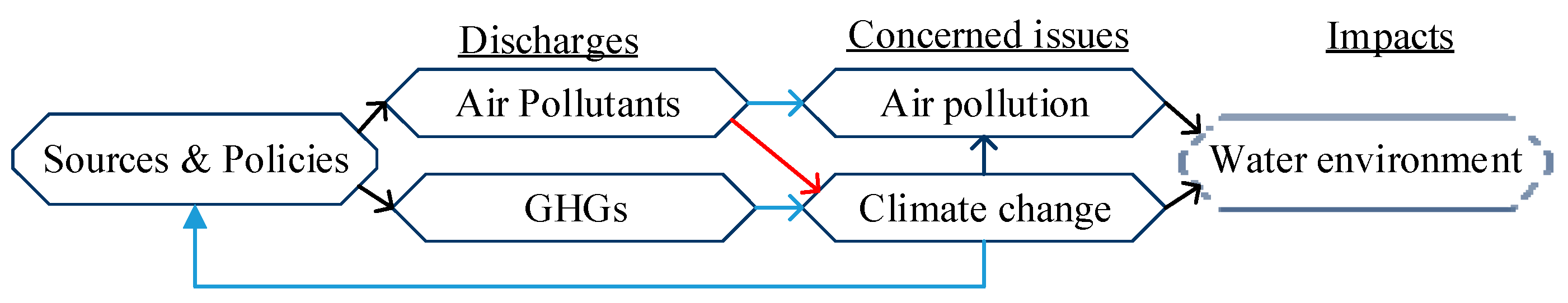
The evolution of technology has increased the use of fossil fuels, which is a major cause of the increase in the concentrations of CO₂ and other greenhouse gases (GHGs). Understanding the environmental impacts of technological changes is essential for sustainable economic growth. Popp et al. [37] indicated that technology transition has largely affected the environment. They conjectured that advanced technology would escalate air pollution. Technological advancement is the most important part in projecting future impact on global environmental challenges, such as climate vulnerability [37]. Climate change is directly linked to air pollutants. Certain pollutants, such as black carbon and ozone, contribute to global warming by trapping heat in the atmosphere (Figure 4).

2.3. Economic Growth

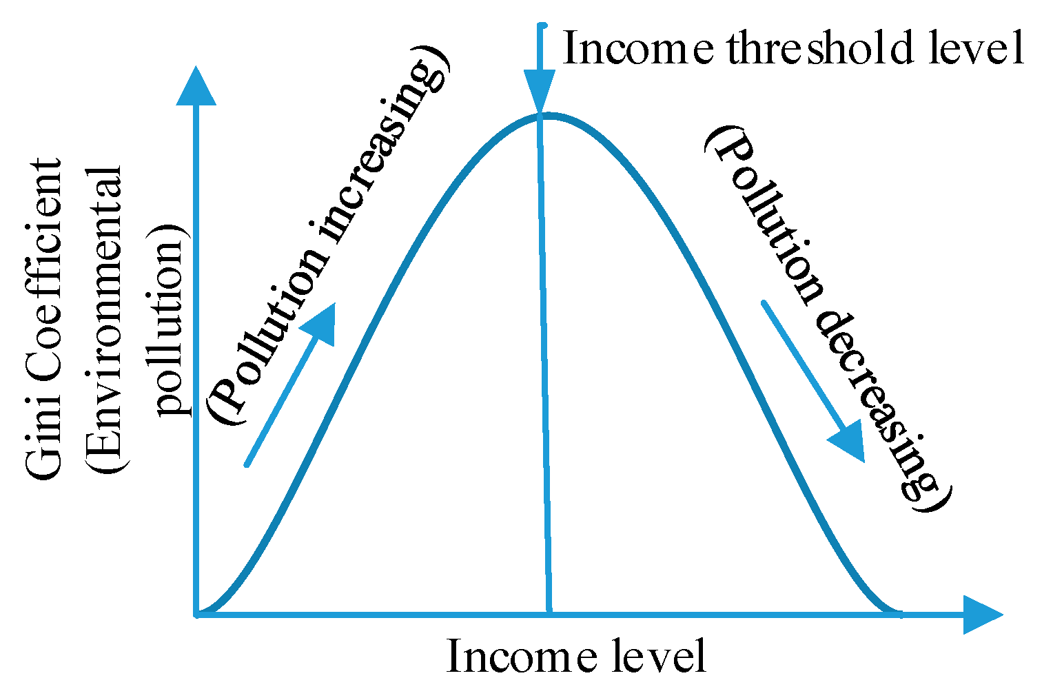
The nexus between economic development (GDP) and environmental sustainability has been long discussed. In particular, environmental objectives such as limiting global warming below a threshold (2 °C or 1.5 °C) have been challenging owing to continuous economic growth [38]. Industrial growth has recently negatively impacted the environment and increased GHG concentrations, toxic pollutants, and chemical spills [39]. Wu et al. [40] hypothesized that income inequality and per capita income have an inverted U-shaped relationship. This indicates that the degree of environmental pollution increases as economic growth approaches the threshold income level and then declines at the same rate (Figure 5).

2.4. Role of Institutions

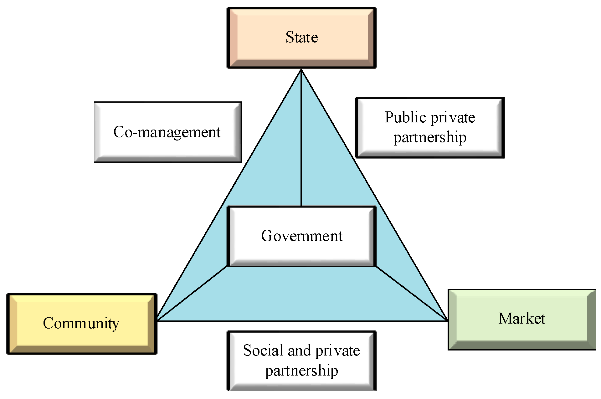
It is vital to effectively address the role of institutions (particularly local ones) in preparation for adaptation to climate variations if this adaptation is to help the most susceptible social groups. Previous research indicates that the success of adaptation normally depends on the type of existing institutions [41]. Conversely, previous research also highlights the factors that resist adaptation and indicates institutional hurdles as a main cause of ineffective adaptation to climate variation [42,43,44,45]. The failure of institutions to adapt to climate change has aggravated their climate vulnerability (Figure 6).

Table 1. Summary of recent studies on major climate variability-forcing drivers.

Driver	Major Findings	Methodologies/Techniques	References
Population growth/Urbanization	Role of urbanization growth on pollutants emissions and energy intensity development Effects of urbanization and energy growth on China’s environment Population increase and urbanization implications for climate change Greatly rising water needs, greenhouse warming	Panel data techniques, Mean group estimation Theoretical modeling approaches Statistical approaches Numerical analyses, climate models	[35] [46] [47] [48] [49]
Technologic development	Carbon dioxide emissions in relation with technology change Possible environmental risks by large-scale seawater desalination plants Environmental change in response to technology evolution Impact of technological advancement on photosynthesis phenomenon	Empirical analyses, dual effects model Conceptual models, statistical approaches Theoretical and numerical models Agrometeorological model	[50] [51] [37] [52]
Economic growth	Proposed relation between urbanization, economic development and environmental vulnerability Public perception against economic growth and environmental pollution. Developed a relation between CO2 emissions and economic growth in EU-5 U-shaped relation between environmental deterioration indicators and per capita income.	Theoretical and simulation equation models, Empirical simulation Statistical analyses Empirical methods Linear model	[53] [54] [55] [56]
Institutions	Institutional challenges against climate change to improve agricultural productivity Efficiency of formal institutions to mitigate climate change impact Facilitating in local level adaptation by the public/private institutional arrangements Effectiveness of local institutions in adaptation to climate variation	Qualitative methods Conceptual models Qualitative approaches Qualitative and quantitative analyses	[57] [58] [59] [60,61]

Table 1. Summary of recent studies on major climate variability-forcing drivers.

Driver	Major Findings	Methodologies/Techniques	References
Population growth/Urbanization	Role of urbanization growth on pollutants emissions and energy intensity development Effects of urbanization and energy growth on China’s environment Population increase and urbanization implications for climate change Greatly rising water needs, greenhouse warming	Panel data techniques, Mean group estimation Theoretical modeling approaches Statistical approaches Numerical analyses, climate models	[35] [46] [47] [48] [49]
Technologic development	Carbon dioxide emissions in relation with technology change Possible environmental risks by large-scale seawater desalination plants Environmental change in response to technology evolution Impact of technological advancement on photosynthesis phenomenon	Empirical analyses, dual effects model Conceptual models, statistical approaches Theoretical and numerical models Agrometeorological model	[50] [51] [37] [52]
Economic growth	Proposed relation between urbanization, economic development and environmental vulnerability Public perception against economic growth and environmental pollution. Developed a relation between CO2 emissions and economic growth in EU-5 U-shaped relation between environmental deterioration indicators and per capita income.	Theoretical and simulation equation models, Empirical simulation Statistical analyses Empirical methods Linear model	[53] [54] [55] [56]
Institutions	Institutional challenges against climate change to improve agricultural productivity Efficiency of formal institutions to mitigate climate change impact Facilitating in local level adaptation by the public/private institutional arrangements Effectiveness of local institutions in adaptation to climate variation	Qualitative methods Conceptual models Qualitative approaches Qualitative and quantitative analyses	[57] [58] [59] [60,61]

3. State-of-the-Art Methodology

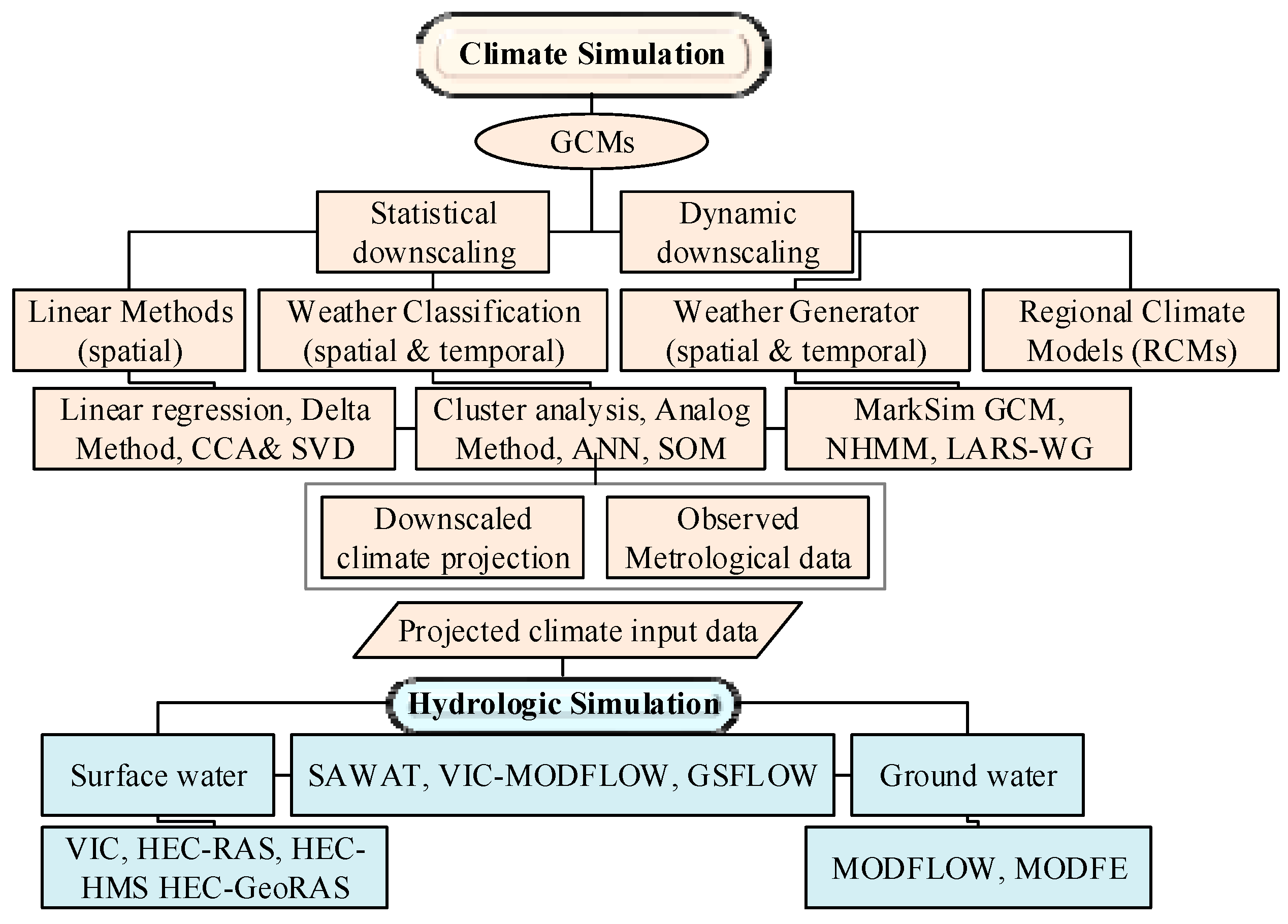
To assess the impact of climate on water resources and hydrology, it is necessary to first compute rainfall–runoff, analyze temperature variations, compute population increases within the basin, and then statistically evaluate the results [62,63]. Progressive downscaling approaches that can be used on the temporal and spatial aspects of climate have been used for projected climate scenarios. Statistical downscaling models are relatively computationally effective and have been applied on a large scale to determine the impacts of regional climate change, particularly in hydrological response evaluations [64]. Trzaska and Schnarr [65] categorized statistical approaches as linear methods (canonical correlation analysis), weather classifications (artificial neural network), and weather generators (non-homogeneous hidden Markov model (NHMM)). A conceptual methodological framework is shown in Figure 7.

3.1. Determination of Variations in Climatological Parameters

Only cortical rain gauges have been used to collect the daily rainfall data [15,62,66]. Then, annual and seasonal rainfall was aggregated. However, there are two methods to identify the temperature and precipitation variations linked to climate change. Let us consider the hypothetical temperature and precipitation variations. Alternatively, data from the general circulation model (GCM) can be utilized [7,9,67]. Temperature is a crucial factor in regional meteorological variation.

GCMs depict connected atmosphere–ocean–ice–land systems. These models show how the atmosphere reacts to varying greenhouse gas concentrations [68,69,70,71]. Furthermore, a review of previous studies can help identify the most trustworthy and accurate GCM [72,73,74]. However, the geographical and temporal resolution of the GCM output data does not fulfill the hydrological model resolution criteria. The spatial resolution (approximately 100–300 km) is insufficient for handling complex hilly terrain and sub-framework scale events such as convective precipitation.

Table 2. State-of-the-art methods used to simulate climatological variables.

Climatological Parameters	References	Methods Used	Major Findings
Precipitation	[75] [76] [77] [78]	Empirical modeling, theoretical approaches Intensity duration frequency (IDF) curves Simulation modeling approaches Integrated hydrological modeling; HydroGeoSphere (HGS)	Determined the rainfall intensity and average volume diameter Evaluated properties of hourly rainfall Estimated rainfall variation under climate change in different regions of UK Evaluated hydrological system in glacial regions
Temperature variation	[79] [80] [81]	RS and GIS; Landsat-8 GCMs through representative concentration pathways ANOVA, and Mann–Kendall trend test	Measurement of temperature and land surface process Evaluated temperature and precipitation variation Pattern of temperature change and rainfall behavior
Air humidity	[82] [32] [32]	Hygrometer, psychrometers, dew-point meter, evaporimeter and atmometer Three-dimensional computational fluid dynamics (CFD) modeling Humidity meter	Air humidity measurements Numerical prediction of air humidity Measured relative air humidity
Wind speed/wind direction	[83] [84] [85]	Linear multivariable model Time series models; mathematical model Time series method; empirical Bernstein copulas	Proposed idea of wind speed estimation Determined mean wind speed per hour Wind direction/wind speed simulation
Solar/terrestrial radiation	[86] [87] [88]	Commercial pyranometers Pyrheliometer, different modeling approaches Plastic scintillation counter High-purity germanium (HPGe) detector	Determined solar irradiance Solar and infrared radiation measurements Determined Terrestrial γ radiation Figured out environmental radioactivity

summarizes the current climate simulation research.

3.2. Hydrologic Simulation

The climatological data of the first step (namely, temperature and precipitation) are then utilized to construct a hydrological model that forecasts fluctuations in hydrological parameters (i.e., infiltration, runoff, and evapotranspiration). Statistical hydrological models can be used to forecast future runoff values based on the characteristics of historical data. Models that characterize the relationship between streamflow runoff and climate factors (through regression or observational analysis) are examples of statistical models used to estimate the impact of climate change [89].

Table 3. State-of-the-art methods used for rainfall runoff simulation since 2018.

References	Methods	Key Objectives	Major Findings/Contribution
1. [32] 2. [17] 3. [90] 4. [7] 5. [91] 6. [92]	Fourier–Stieltjes representation approach Neuro-fuzzy setup for R-R modeling A method based on the integration of an adaptive neuro-fuzzy inference system (ANFIS) with principal component analysis (PCA) SWAT model Neuro-fuzzy setup for R-R modeling Stochastic modeling by using Fourier–Stieltjes representation technique	To evaluate changes in runoff discharge Rainfall–runoff modeling Runoff flow estimation Rainfall–runoff simulation in karst topography, curve number (CN) performance validity Time-based rainfall–runoff relationship Runoff modeling for small watersheds	Found that runoff discharge changes with the characteristic catchment size and rainfall time scale. Rainfall–runoff (R-R) model was calibrated in three various catchments kinds and sizes, and the results were compared with physical models. Emphasized flow routing aspects by challenging the GIS use based on the handling of rainfall input data. Predicted peak flow in Lijiang river basin. Performed streamflow simulations in different land use water basins. Concluded that: Runoff variability increases with rainfall time-scale characteristics variability; Constant mean travel time reduces the runoff discharge variability.

summarizes the current rainfall–runoff simulation research.

4. Consequences for Water Resources

Global warming is detrimental to the global freshwater supply. It has altered the overall hydrological cycle and, thereby, altered the quality, quantity, distribution, and timing of the available freshwater [93]. Water shortages are increasing constantly as a result of climate change, river discharge magnitudes and shifts, and population growth dynamics [49,94,95].

Deng et al. [75] illustrated that data from meteorological stations play a vital role in the study on climate variation vulnerability by providing better future climate projections and wet–dry conditions. Zhang et al. [32] examined data from the past 50 years collected from an arid region of the northwest. It was observed that most of the observation stations are established in lower elevation regions, and their number is small in hilly terrains. It is important to understand the hydrology of mountainous regions for long-term watershed management and sustainable water availability. In terms of water resource availability, downstream catchments are intimately linked to variations in precipitation and temperature at the upstream catchments [89,96]. Recent studies on the effects of climate change on water resources are summarized in

Table 4. State-of-the-art research on climate variability and subsequent effects on water resource.

Response	References	Key Objectives	Impacts on Water Resources and Hydrology	Methods Used	Remarks
Global temperature change	[97] [98] [99] [100]	1. To account for non-climatic influences in assessments of variations in global surface air temperature. 2. Global and hemispheric surface trend analysis, as well as annual temperature anomalies. 3. Prediction of global surface air temperature equilibrium changes. 4. To examine the effects of rising CO2 levels in the atmosphere on world hydrology.	In 2000, the global temperature is moderately high in the Pacific Ocean. Between 1861 and 2000, the global surface temperature increased by 0.61 0.16 °C. The subsequent reaction of precipitation to global surface–air–temperature change is 2–3 percent K-1. In the 2CO2 experiment, the global and annual mean near-surface temperatures increased by 2.42 K.	GIS Analysis Optimal average technique Atmospheric model based on Hadley Centre’s GEM climate model Model of the overall circulation of the atmosphere Community Climate Model (CCM3)	The global land surface, ocean, and air temperature have significantly increased over the last two centuries.
Warming oceans	[101] [102] [103] [3]	1. To intensify the shifts in poleward warming due to an increase in greenhouse gases. 2. Ocean acidification’s effects on marine organisms in conjunction with global warming. 3. The role of non-genetic and genetic inheritance in determining organisms’ adaptive capability in a warming ocean scenario. 4. The link between ENSO Modoki and conventional ENSO and the frequency of tropical cyclones (TCs) in the western North Pacific.	Accelerated warming in the Southern Ocean or a strong poleward spread of warmth as emissions increase. Reductions in survival, calcification, development, and abundance of marine creatures as a result of ocean acidification. Transgenerational effects could be extremely effective at mitigating the effects of ocean warming if temperature increases gradually. The effect of ENSO Modoki on TC activity should be considered when predicting TC activity in the context of global warming or when the region’s WNP negative heating anomaly is removed.	The Hadley Centre’s Sea Ice and Sea Surface Temperature datasets are examples of observed SST datasets. Meta-analysis Transgenerational plasticity (TGP) and quantitative genetics Simple baroclinic model	Warming oceans lead to sea-level rise; moreover, hot oceans carry more CO2, which causes seawater to become more acidic.
Shrinkage ice and glacier retreat	[104] [105] [106] [105]	1. Mass balance study of four Kangri Karpo glaciers. 2. Acceleration of glacier retreat in non-polar areas over the twentieth century. Affected South Asian Rivers by Himalayan Glacier Melt 3. Earth sciences and water resources include studying the hydrological cycle and snow and ice.	The study discovered a significant loss of ice mass and rapid glacier retreat since the 1980s. There has been widespread observation of broad glacier retreat that has been significantly more rapid since the mid-1970s. Due to increase in monsoonal precipitation and rise in temperature, the flow along the Himalayas arc increases by enhanced glacier ice melt. Overall statement of prevalent glacier retreat is significantly quicker since the mid-1970s.	Observation of glacier mass combined with detailed study Physical processes (melting and sublimation) Rating curve method, bulk hydrograph, cross-sectional measurements are being used. Modeling studies, field measurements	A significant ice and glacier retreat have been seen since the 1970s.
Sea-level rise	[107] [108] [109] [110]	1. Relationship between global sea level variation and global mean temperature. 2. The economic costs of climate change and benefits of adaptation at the city scale. 3. The impact of rising sea levels on predicted storm surge water levels and frequency. 4. Estimating SLR to estimate coastal recession.	Sea level is rising from (75–190) cm for period 1990–2100. Rising sea levels would exacerbate flood hazards. It is based on an empirically determined link between temperature changes and sea-level rise. The only climate change impact that is considered is sea-level rise.	Climate Model, R07 Rising sea levels increase flood risk. An empirical link between temperature and sea-level rise underpins it. Simple, deterministic method (Bruun rule), PCR model, probabilistic model, Dune erosion model	A substantial nexus between temperature change and sea-level rise has been seen. From the late 19th century, the sea level rises significantly, which is likely to exacerbate hydro-hazards.
Extreme events	[111] [112] [113] [114]	1. Impacts of changing extreme weather and climate events. 2. In the absence of major anthropogenic warming, the best technique to analyze possible climate change impacts on disaster losses. 3. Weather and climate extremes changes (frequency and temperature distribution). 4. Changes in climatic extremes owing to anthropogenic CO2 and aerosol emissions.	Extreme occurrences will become more often, and societal infrastructure will become increasingly vulnerable to weather and climatic extremes. It has been determined that anthropogenic climate change has had a major impact on economic losses caused by various weather-related natural disasters around the world. It will have an impact on society and the ecosystem. A rise in heatwave episodes across terrestrial areas is likely.	Climate model studies Systematic analysis or studies Climate model, statistical characteristics Dynamical or statistical downscaling coupled with atmosphere–ocean general circulation models.	In extreme weather events, hydro-hazards (i.e., floods and droughts) are more likely to occur now and in the future.
Ocean acidification	[115] [102] [107] [116]	1. Additional strategies to mitigate the potentially harmful effects of climate change in coastal marine systems are being developed. 2. Occurrence of changes in marine ecosystems are caused by global warming and acidification. 3. Global changes in parameters such as temperature, currents, and sea level fluctuation on coral reefs due to ocean acidification have unknown effects. 4. Productivity and the relationship between corals and their symbiotic dinoflagellates. Reduced calcification rate of framework builders is a major threat to coral reefs. Examining the effects of bleaching state on organic productivity, which is expected to be influenced, and comparing the patterns of organic responses with effects on calcification rates.	It has been observed that climate shifts may result in large-scale community alterations. Why ocean acidification may reduce biodiversity and profoundly alter ecosystems; therefore, understanding how it affects creature fitness, sustenance, and success is crucial with this research approach. It causes bleaching (pigmentation loss) in two important types of reef-building animals, as well as decreased productivity in coral reef builders.	Physiological, morphological, and behavioral effects and transport processes Conceptual model, physiological principles Intertidal and subtidal SCUBA surveys, short-term laboratory experiments Effects of experimental ocean acidification	Changes in pH due to ocean acidification are altering water ecosystems and functions.
Decrease in snow cover	[117] [118] [119] [120]	1. In the Swiss Alps, the duration of snow cover is rapidly decreasing, as is the maximum HS and the frequency of DSP. 2. Multi-dataset calibration using a quantile mapped ensemble of climatic states to generate watershed discharge scenarios. Multiple datasets were used to calibrate the hydrological model. 3. The impact of four statistically determined coming climate events on water resources toward the end of the twenty-first century. 4. Spatial and temporal variability of snow cover and snow water equivalent over Eurasia.	The snowpack reduction is most likely associated with the elevation increase in temperatures. The uncertainty in the glacial runoff was considerably reduced by linking the multi-dataset calibration. Due to the rising temperatures brought on by a changing climate, annual peak runoff occurs sooner. Temperature trends that vary from year to year or season to season	A bootstrap method Use of daily/annual HS data, filtering procedure HBV-light model, digital elevation models (DEMs), analysis of variance (ANOVA) GCM downscaling, future snowpack estimation, and runoff simulation NSIDC EASE-grid weekly SCE and monthly SWE data reliability and possible uncertainties	Snow melting has altered peak runoff timing, and the uncertainty in the glacial runoff is significantly reduced.

.

As global temperatures rise, more water evaporates, increasing atmospheric water vapor and more frequent, heavy, and severe storms in the coming years [97,98,99,100]. Hotter oceans can hold more CO₂, causing seawater to become more acidic [101,102,103]. Rising temperatures cause alpine glaciers to melt, changing water availability to cause flooding [104,105,106]. Initially, when the glacier melts, more water flows downhill away from it. However, as the glacier melts, the water supply will be reduced, and farms, villages, and towns may lose an essential water source [107,108,109,110]. Moreover, extreme weather events can also have an impact on water security. Problems can emerge from too much water, such as flooding, or too little water, such as droughts. Water resources will therefore decline as the seasonal snowpack declines and glaciers disappear. Furthermore, rapid snow melt in the spring can cause flooding, whereas delayed melting of snow and ice allows water to penetrate the ground [111,112,113,114].

4.1. Impact on Hydrological Regime

Regional hydrological regimes have been altered or would be transformed because of climate change. Previous research has shown the influence of climate change on surface and groundwater, both at present and in the future [121,122]. Understanding river flow patterns is critical to watershed management and long-term sustainability. Pumo et al. [123] observed that the hydrological regime influences the form and behavior of river basins. However, meteorological factors (such as precipitation frequency and intensity) as well as seasonality influence streamflow regimes. Climate change influences precipitation intensity, magnitude, timing, and frequency [115]. According to NASA’s latest assessment, storm-affected areas would experience more precipitation, whilst locations further from storm tracks are likely to see less precipitation and an increased risk of drought. In the future, climate change would have a significant impact on streamflow systems worldwide.

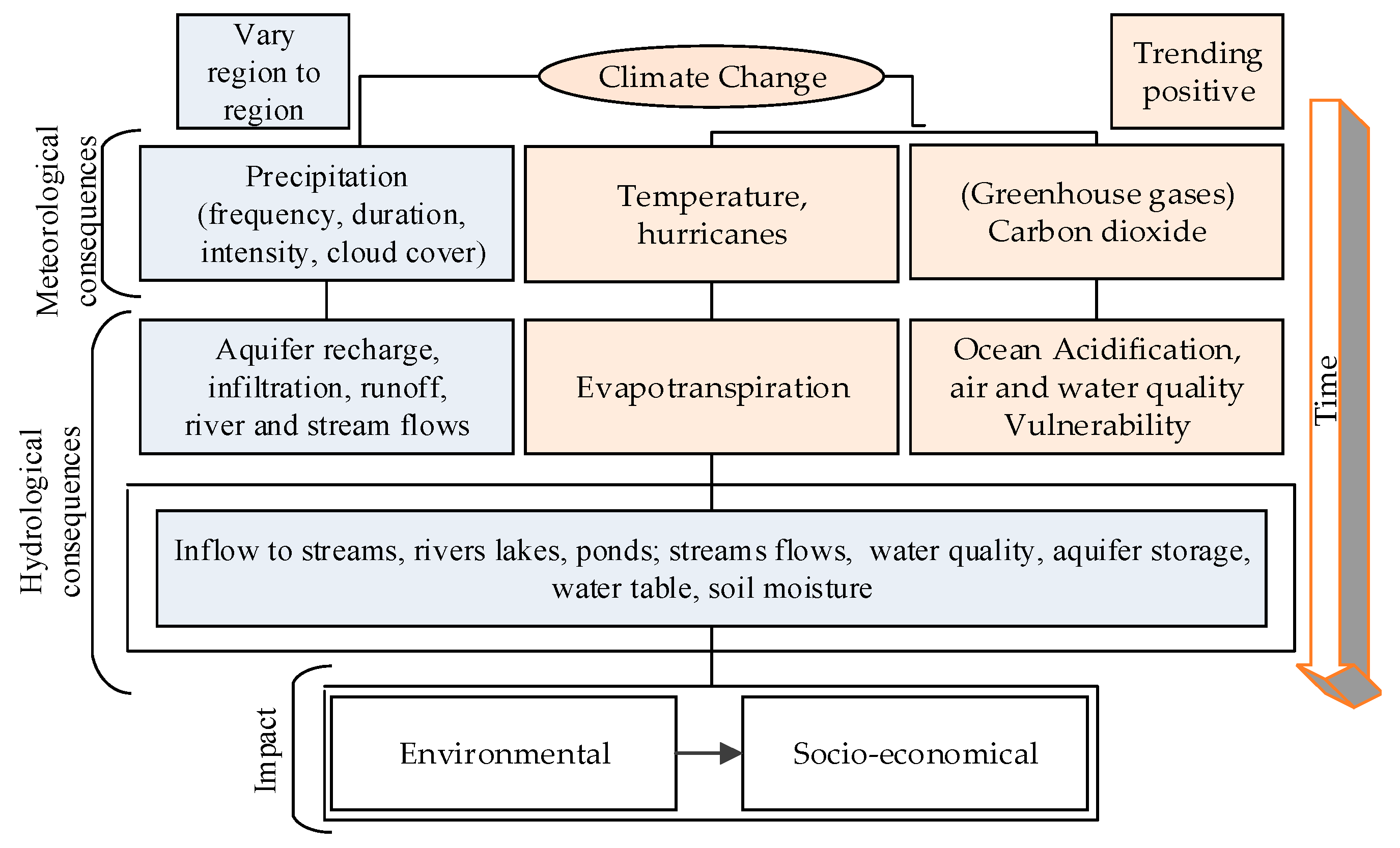
Generally, the critical global projections from the prior discussions are: (i) by 2100, average global temperatures are anticipated to rise by 0.5 °F to 8.6 °F, with a significant increase of at least 2.7 °F across all scenarios except the areas where greenhouse gas emission mitigation strategies are most active; (ii) precipitation patterns and storm occurrences, including rain and snowfall, are also likely to shift. Some of these changes, however, are less clear than those linked with temperature. According to projections, future precipitation and storm changes are expected to differ by season and region: (iii) future projections of sea-level rise vary from region to region. Still, the worldwide sea level is expected to increase faster in the next century than in the previous 50 years; (iv) glaciers are predicted to continue shrinking in size. The degree of melting is likely to accelerate further, contributing to sea-level rise; (v) the pH of the oceans is likely to fall even further by the end of the century as CO₂ concentrations rise in the near future; and (vi) the occurrence, magnitude, and duration of extreme events (i.e., floods and droughts) will increase in the future. Figure 8 shows the trends of the hydro-climatic variables.

4.2. Impact on River-Flow System

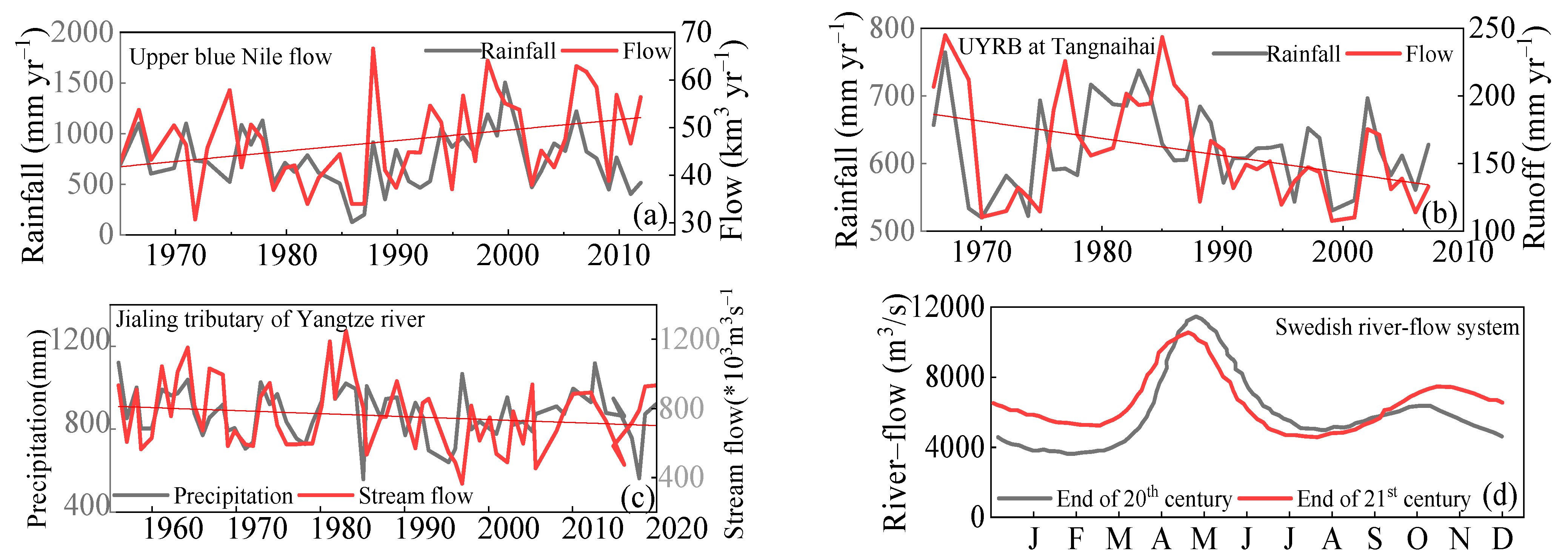
The impact of climate change on river-flow systems varies from region to region. The upper Blue Nile shows positive trends in the 30-year moving averages of the mean and standard deviation of annual river flow and annual rainfall (Figure 9a) [124]. Conversely, the Tangnaihai tributary of the upper Yellow River basin (UYRB) shows a significant decrease in a runoff with the rate of −11.6 mm/decade (Figure 9b) [125], and Jialing tributary of the Yangtze River basin shows a negative trend in average annual streamflow with a change rate of 1572.3 (m³/s)/a (Figure 9c) [126]. Similarly, the flow peak (mean annual maximum flow) was found to be lowered by 15% across Sweden, and the annual redistribution of overall river flow to the sea accounts for 19% on average. Surprisingly, the same changing pattern is shown for the projected climate of the same region (Figure 9d) [127].

5. Worldwide Examples Showing Hydrological Impacts Caused by Climate Change

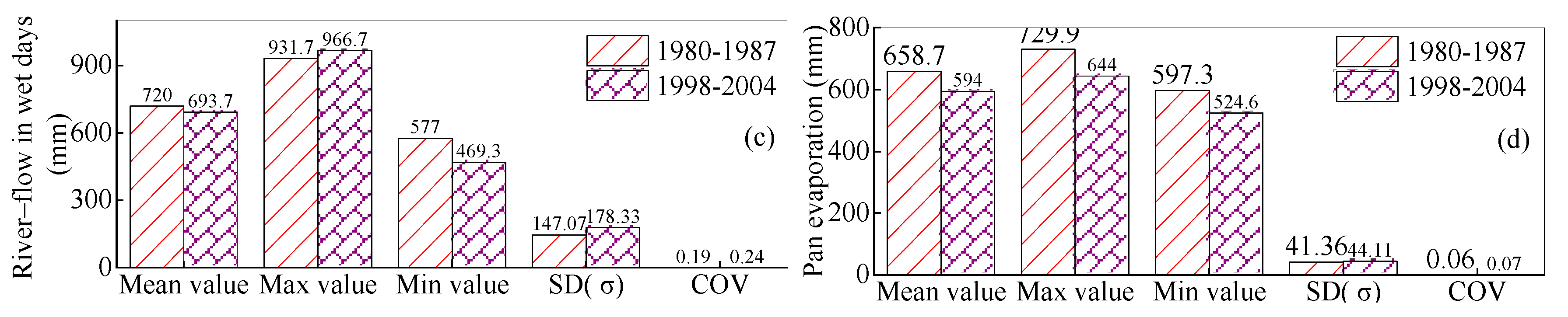
Example 1: Qingyi River watershed, China. The Qingyi River watershed is a pronounced hilly region upstream of the Yangtze River in China [128]. Climate change influences the hydrology of watersheds, particularly surface runoff variability. The water levels reduced dramatically from 1980 to 2004 [129,130,131]. Annual precipitation decreased significantly. Considering climate change, Liu et al. [132] concluded that increased precipitation on the western side of the watershed increases annual surface runoff, base flow, and evapotranspiration by 13%, 8.7%, and 1.1%, respectively. Furthermore, in the central region, evapotranspiration and surface runoff decreased significantly in the southeast. However, the increase in base flow was less, owing to variations in temperature and precipitation.

Evapotranspiration increased by 0.2% in the central region, owing to the substantial decrease in precipitation. The high temperature increased evapotranspiration. Moreover, evapotranspiration decreased by 3.1%, notwithstanding increased temperatures and precipitation to the northwest of the watershed. The variations in temperature, streamflow, and evapotranspiration are shown in Figure 10.

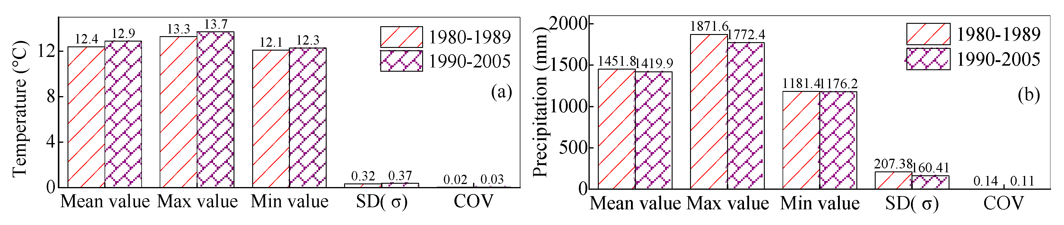
Example 2: US Mid-Atlantic region. The Mid-Atlantic is likely to show an increase in both temperature (T) and precipitation (P). However, the magnitude and direction of the increase varies between GCMs [131,132]. Precipitation (P) varied negligibly across the watersheds of the region, with a 1% coefficient of variation (COV) annually and seasonally [133]. The annual precipitation depth did not vary. However, the annual humidity and fall transition duration varied, and the non-growing and growing seasons were drier [134]. The watersheds exhibited similar variations in all the scenarios. Thus, evapotranspiration was affected more by temperature, humidity, cloud cover, and wind speed. The statistical tests showed a positive variation of 8% in temperature.

The water yield decreased in all the watersheds during the non-growing season. The parameter that varied the most was runoff, with COVs of 7%, 23%, and 26% in spring, growing season, and fall transition, respectively. The average annual runoff in the ten Mid-Atlantic watersheds was 1.05 mm/day, with a COV of over 9%. The statistics for the Cub and Cedar watersheds are shown in

Table 5. Statics for seasonal variability of precipitation (P), runoff (R), evapotranspiration plus change in storage (ETDS), and water yield (WY) for Cub watershed (Data source; [133]).

Time Periods	Statistic	P (mm)	R (mm)	ETDS (mm)	Cub Run WY (mm)	Cedar Run WY (mm)
Annual	Mean	3.05	1.11	1.98	0.35	0.32
	Median	2.99	1.11	2.02	0.33	0.29
	SD	0.35	0.47	0.24	0.10	0.12
	COV (%)	17.3	42.4	12.2	27.9	38.9
Non-growing season	Mean	2.53	1.44	1.11	0.55	0.57
	Median	2.38	1.37	1.09	0.57	0.58
	SD	0.68	0.65	0.41	0.17	0.23
	COV (%)	26.8	45.1	37.1	29.8	40.7
Spring transition	Mean	3.02	1.61	1.45	0.51	0.48
	Median	2.95	1.39	1.52	0.46	0.46
	SD	0.99	0.85	0.49	0.16	0.21
	COV (%)	32.7	52.6	33.5	31.5	43.0
Growing season	Mean	3.34	0.75	2.62	0.21	0.15
	Median	3.27	0.61	2.58	0.18	0.13
	SD	1.19	0.54	0.62	0.11	0.11
	COV (%)	35.5	71.7	23.8	54.1	73.3
Fall transition	Mean	3.19	0.92	2.26	0.25	0.17
	Median	3.39	0.86	2.18	0.22	0.13
	SD	1.09	0.79	0.64	0.15	0.17
	COV (%)	34.2	85.9	28.1	60.3	95.1

.

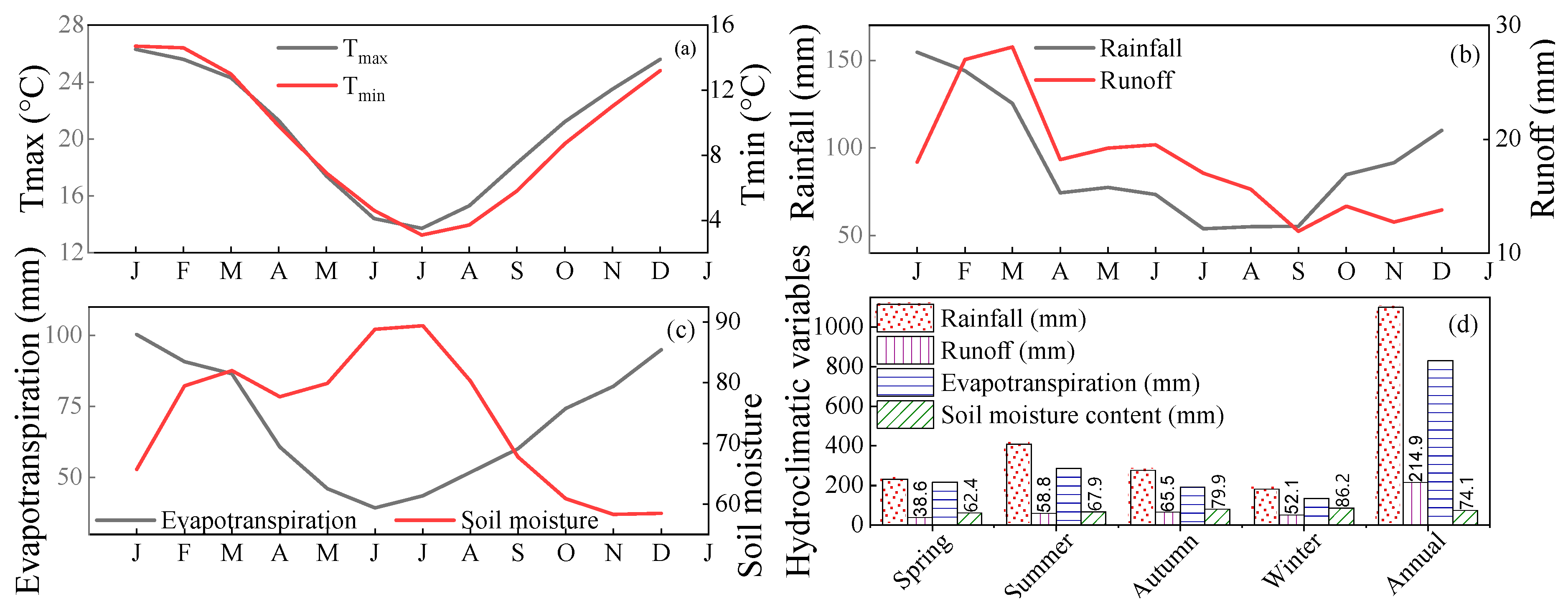
Example 3: Manning River basin, Australia. Australia is referred to as the continent with the most variable climate [81]. This has had a significant impact on the country’s water resources and ecosystem health. The Manning River basin is located on the central north coast of New South Wales and has a catchment area of 6630 km². Zhang and Huang [135] determined that the mean annual temperature and mean evaporation of Manning River basin for 1977–2016 were 14.9 °C and 1305 mm, respectively. The basin receives an average rainfall of 1052 mm and has a runoff coefficient of 0.2.

Zhang et al. [32] determined that temperatures would be higher in the 2080s than in the 2040s on seasonal and monthly timescales. The largest median would increase by 1.6 °C by November 2040 and 3.8 °C by September 2080 for maximum monthly temperatures. In contrast, the lowest median temperature increase would be 1.1 °C by March 2040 and 2.5 °C by February 2080. On a seasonal scale, temperatures are likely to increase (a median increase of 1.5 °C by 2040 and 3.4 °C by 2080) in spring for both periods. Meanwhile, these are likely to decrease in the autumn of 2040 (1.3 °C) and summer of 2080 (2.9 °C). In addition, the projected largest runoff (monthly) is likely to shift from March to February compared with the baseline. The projected maximum monthly increase in runoff would be 6.9% in November 2040 and 31.1% in February 2080. Meanwhile, the maximum monthly decrease would be −16.7% in June 2040 and −205% in July 2080. Figure 11 illustrates the variability of hydrological and climatological variables in the Manning River basin.

6. Evaluation and Management of Water Resources

According to the aforementioned analysis, effective management of water resources is urgently required [30,136,137] against the stress of climate change, unequal temporal and spatial distributions, pollution, and overexploitation of water reserves [21,135,136,137,138,139,140,141,142]. Based on environmental risk assessments [20,104,143,144,145,146,147,148,149], resource evaluation management methods [7,150,151,152] should be applied to ensure the efficient utilization of water resources [153,154,155]. To save time and energy, it is necessary to switch from traditional to modern ways. In practice, the heat flow method or the thermal storage volume approach based on a shallow geothermal survey is frequently used to estimate the quantity of water resources. [156,157,158,159]. Shallow geothermal surveys including geological and geothermal field surveys partially follow conventional geothermal survey methods such as field investigations [160,161,162], drilling surveys, and laboratory or field tests [163,164]. Certain new innovative evaluation systems need to be proposed to replace the conventional approaches adopted in water resource management. This is because the water resource investigation’s objective and task, considering climatic change, differ from the conventional ones.

Water resource monitoring and prediction are two significant aspects of risk evaluation [165,166,167]. Geographical information systems (GISs) and artificial intelligence (AI) are two remarkable technologies presently available in the field of resource evaluation and management. Assessments of water resource potential are based predominantly on GIS data. Many AI technologies can be used for resource evaluation and management, including the analytic hierarchy process (AHP) approach [145,168], deep learning neural networks, and long short-term memory (LSTM) [150,151,152]. Prior investigation is necessary to ensure the suitability of a specific AI method for the problem at hand. Therefore, it is important to consider the special characteristics of related problems [169]. The application of AI methods to water resource evaluation will become an important research area in the future [170,171,172].

7. Conclusions

This study summarized the impacts of climate change on water resources, hydrological patterns, and the key drivers of climate change. The review results indicate that climate change affects water resources more adversely than other deteriorating factors. The climate change scenarios affect evapotranspiration, precipitation, base flow, inflow to streams and rivers, and streamflow. Based on the above reviews, the main conclusions of this study are as follows:

(1)

The fast-growing population has increased the rate of urbanization, economic growth, and technological development. This is causing a significant increase in the concentration of GHGs in Earth’s troposphere because of inadequate mitigation and adaptation measures. The temperature of the planet has increased owing to the increase in CO₂ and other GHGs. Climate variability is a key consequence of abrupt increases in temperature and GHG emissions. It affects water reserves and the overall environment. However, a lack of mitigating institutions and people’s lack of environmentally friendly attitudes have increased climate vulnerability.

(2)

The variation in hydrological patterns and the water crisis are measured in two steps: (1) assess regional and local variations in climatological variables (i.e., temperature, precipitation, air humidity, and wind speed), and (2) evaluate the resulting pressure on hydrological parameters (i.e., runoff, inflow to streams and rivers, streamflow, base flow, and soil moisture) and water resources.

(3)

The literature review revealed that the temperature of Earth has been increasing regularly. The average global temperature has increased by 0.8 °C (1.4 °F) since 1880. This increase has adversely affected Earth’s overall climate by causing frequent and abrupt extreme events (such as droughts, floods, hurricanes, tornadoes, and acid rain). However, the precipitation rate (particularly rainfall) has decreased in certain local and regional scenarios. This may cause freshwater scarcity in the future.

(4)

There is a strong relationship between the climatic variables and hydrological patterns. Increases in temperature and decreases in precipitation reduce surface runoff. This would result in low inflows to streams and rivers. In addition, soil moisture and infiltration rates would decrease. This implies that groundwater aquifers are not being recharged and that aquifer water budgets have been disturbed, thereby lowering the groundwater table. However, the increase in temperature has enhanced the melting rate of snow, ice, and glaciers at high altitudes. This has resulted in an average annual increase in sea level by 1.2–1.7 mm since 1900 and by 3.2 mm since 2000.

(5)

Climate variability has also caused deterioration in surface and ground water quality. Saltwater from the seas intrudes into fresh aquifers in coastal areas, owing to the decrease in groundwater level and increase in sea level. Saltwater intrusion affects the quality of groundwater. Similarly, in certain scenarios, freshwater quality has also been disturbed by acid rain caused by the high concentration of CO₂ in the atmosphere.

References

- Milly, P.C.D.; Dunne, K.A.; Vecchia, A.V. Global pattern of trends in streamflow and water availability in a changing climate. Nature 2005, 43, 347–3508. [Google Scholar] [CrossRef] [PubMed]
- Moglen, G.E.; Rios Vidal, G.E. Climate change and storm water infrastructure in the mid-Atlantic region: Design mismatch coming? J. Hydrol. Eng. 2014, 19, 4014026. [Google Scholar] [CrossRef]
- Chen, H.; Xu, C.-Y.; Guo, S. Comparison and evaluation of multiple GCMs, statistical downscaling and hydrological models in the study of climate change impacts on runoff. J. Hydrol. 2012, 434, 36–45. [Google Scholar] [CrossRef]
- Chai, J.C.; Shen, S.L.; Geng, X. Effect of initial water content and pore water chemistry on intrinsic compression behavior. Mar. Georesour. Geotechnol. 2019, 37, 417–423. [Google Scholar] [CrossRef] [Green Version]
- Lin, S.S.; Shen, S.L.; Lyu, H.M.; Zhou, A. Assessment and management of lake eutrophication: A case study in Lake Erhai, China. Sci. Total Environ. 2021, 751, 141618. [Google Scholar] [CrossRef]
- Fatichi, S.; Rimkus, S.; Burlando, P.; Bordoy, R. Does internal climate variability overwhelm climate change signals in streamflow? The upper Po and Rhone basin case studies. Sci. Total Environ. 2014, 493, 1171–1182. [Google Scholar] [CrossRef]
- Lyu, H.M.; Shen, S.L.; Zhou, A.; Zhou, W.H. Flood risk assessment of metro systems in a subsiding environment using the interval FAHP–FCA approach. Sustain. Cities Soc. 2019, 50, 101682. [Google Scholar] [CrossRef]
- Wu, M.; Hu, Y.; Wu, P.; He, P.; He, N.; Zhang, B.; Zhang, S.; Fang, S. Does soil pore water salinity or elevation influence vegetation spatial patterns along coasts? A case study of restored coastal wetlands in Nanhui, Shanghai. Wetlands 2020, 40, 2691–2700. [Google Scholar] [CrossRef]
- Zhang, X.; Dong, Q.; Costa, V.; Wang, X. A hierarchical Bayesian model for decomposing the impacts of human activities and climate change on water resources in China. Sci. Total Environ. 2019, 665, 836–847. [Google Scholar] [CrossRef]
- Lin, S.S.; Shen, S.L.; Zou, A.; Zhang, N. Ensemble model for risk status evaluation of excavation system. Autom. Constr. 2021, 132, 103943. [Google Scholar] [CrossRef]
- Labat, D.; Godderis, Y.; Probst, J.L.; Guyot, J.L. Reply to comment of Legates et al. Adv. Water Resour. 2005, 28, 1316–1319. [Google Scholar] [CrossRef]
- Labat, D.; Goddéris, Y.; Probst, J.L.; Guyot, J.L. Evidence for global runoff increase related to climate warming. Adv. Water Resour. 2004, 27, 631–642. [Google Scholar] [CrossRef]
- Wu, H.N.; Shen, S.L.; Chen, R.P.; Zhou, A. Three-dimensional numerical modelling on localized leakage in segmental lining of shield tunnels. Comput. Geotech. 2020. 122, 103549. [CrossRef]
- Ranjan, S.P.; Kazama, S.; Sawamoto, M. Effects of climate and land use changes on groundwater resources in coastal aquifers. J. Environ. Manag. 2006, 80, 25–35. [Google Scholar] [CrossRef] [PubMed] [Green Version]
- Zheng, Q.; Shen, S.L.; Zhou, A.; Lyu, H.M. Inundation risk assessment based on G-DEMATEL-AHP and its application to Zhengzhou flooding disaster. Sustain. Cities Soc. 2022, 86, 104138. [Google Scholar] [CrossRef]
- Westerberg, I.K.; Gong, L.; Beven, K.J.; Seibert, J.; Semedo, A.; Xu, C.Y.; Halldin, S. Regional water balance modelling using flow-duration curves with observational uncertainties. Hydrol. Earth Syst. Sci. 2014, 18, 2993–3013. [Google Scholar] [CrossRef] [Green Version]
- Mmeko, M.; Woodhouse, A. Tree-ring footprint of joint hydrologic drought in Sacramento and Upper Colorado river basins, western USA. J. Hydrol. 2005, 308, 196–213. [Google Scholar] [CrossRef]
- Fox, J.P.; Mongan, T.R.; Miller, W.J. Trends in freshwater inflow to san francisco bay from tue sacramento-san joaquin delta. JAWRA J. Am. Water Resour. Assoc. 1990, 26, 101–116. [Google Scholar] [CrossRef]
- Shelton, M.L. Seasonal hydroclimate change in the sacramento river basin, California. Phys. Geogr. 1998, 19, 110–118. [Google Scholar] [CrossRef]
- Shen, S.L.; Atangana Njock, P.G.; Zhou, A.; Lyu, H.M. Dynamic prediction of jet grouted column diameter in soft soil using Bi-LSTM deep learning. Acta Geotech. 2021, 16, 303–315. [Google Scholar] [CrossRef]
- Xu, Y.; Gao, X.; Giorgi, F. Upgrades to the reliability ensemble averaging method for producing probabilistic climate-change projections. Clim. Res. 2010, 41, 61–81. [Google Scholar] [CrossRef] [Green Version]
- Christierson, B.v.; Vidal, J.P.; Wade, S.D. Using UKCP09 probabilistic climate information for UK water resource planning. J. Hydrol. 2012, 424–425, 424–425. [Google Scholar] [CrossRef] [Green Version]
- Arnell, N.W. The effect of climate change on hydrological regimes in Europe: A continental perspective. Glob. Environ. Chang. 1999, 9, 5–23. [Google Scholar] [CrossRef]
- Karlsson, I.B.; Sonnenborg, T.O.; Refsgaard, J.C.; Trolle, D.; Børgesen, C.D.; Olesen, J.E.; Jeppesen, E.; Jensen, K.H. Combined effects of climate models, hydrological model structures and land use scenarios on hydrological impacts of climate change. J. Hydrol. 2016, 78, 535. [Google Scholar] [CrossRef]
- Lyu, H.M.; Shen, S.L.; Zou, A.; Yang, J. Perspectives for flood risk assessment and management for mega-city metro system. Tunn. Undergr. Space Technol. 2019, 84, 31–44. [Google Scholar] [CrossRef]
- Meng, W.L.; Shen, S.L.; Zhou, A. Investigation on fatal accidents in Chinese construction industry between 2004 and 2016. Nat. Hazards 2018, 94, 655–670. [Google Scholar] [CrossRef]
- Liu, J.; Curry, J.A. Accelerated warming of the Southern Ocean and its impacts on the hydrological cycle and sea ice. Proc. Natl. Acad. Sci. USA 2010, 107, 14987–14992. [Google Scholar] [CrossRef] [Green Version]
- Liu, X.X.; Shen, S.L.; Zhou, A.; Xu, Y.S. Evaluation of foam conditioning effect on groundwater inflow at tunnel cutting face. Int. J. Numer. Anal. Methods Geomech. 2019, 43, 463–481. [Google Scholar] [CrossRef]
- Soncini, A.; Bocchiola, D.; Rosso, R.; Meucci, S.; Pala, F.; Valé, G. Water and Sanitation in Multan, Pakistan. In Sustainable Social, Economic and Environmental Revitalization in Multan City; Springer: Berlin/Heidelberg, Germany, 2014; Volume 78, pp. 149–162. [Google Scholar] [CrossRef]
- Chen, Y.L.; Shen, S.L.; Zhou, A. Assessment of red tide risk by integrating CRITIC weight method, TOPSIS-ASSETS method, and Monte Carlo simulation. Environ. Pollut. 2022, 310, 120254. [Google Scholar] [CrossRef]
- Hidalgo, H.G.; Amador, J.A.; Alfaro, E.J.; Quesada, B. Hydrological climate change projections for Central America. J. Hydrol. 2013, 495, 94–112. [Google Scholar] [CrossRef]
- Zhang, H.; Wang, B.; Li L., D.; Zhang, M.; Feng, P.; Cheng, L.; Yu, Q.; Eamus, D. Impacts of future climate change on water resource availability of eastern Australia: A case study of the Manning River basin. J. Hydrol. 2019, 573, 49–59. [Google Scholar] [CrossRef]
- Fonseca, A.R.; Santos, J.A. Predicting hydrologic flows under climate change: The Tâmega Basin as an analog for the Mediterranean region. Sci. Total Environ. 2019, 668, 1013–1024. [Google Scholar] [CrossRef] [PubMed]
- Wang, G.; Yang, P.; Zhou, X. Identification of the driving forces of climate change using the longest instrumental temperature record. Sci. Rep. 2017, 7, 46091. [Google Scholar] [CrossRef] [PubMed] [Green Version]
- Salim, R.; Rafiq, S.; Shafiei, S.; Yao, Y. Does urbanization increase pollutant emission and energy intensity? Evidence from some Asian developing economies. Appl. Econ. 2019, 51, 4008–4024. [Google Scholar] [CrossRef]
- Avtar, R.; Tripathi, S.; Aggarwal, A.K. Assessment of energy-population-urbanization nexus with changing energy industry scenario in India. Land 2019, 8, 124. [Google Scholar] [CrossRef] [Green Version]
- Popp, D.; Newell, R.G.; Jaffe, A.B. Energy, the environment, and technological change. Handb. Econ. Innov. 2010, 2, 873–937. [Google Scholar] [CrossRef]
- Antal, M.; Van Den Bergh, J.C.J.M. Green growth and climate change: Conceptual and empirical considerations. Clim. Policy 2016, 16, 165–177. [Google Scholar] [CrossRef]
- Peng, Y.S.; Lin, S.S. Local responsiveness pressure, subsidiary resources, green management adoption and subsidiary’s performance: Evidence from taiwanese manufactures. J. Bus. Ethics 2008, 79, 199–212. [Google Scholar] [CrossRef]
- Wu, X.; Shen, Z.; Liu, R.; Ding, X. Land use/cover dynamics in response to changes in environmental and socio-political forces in the upper reaches of the Yangtze river, China. Sensors 2008, 8, 8104–8122. [Google Scholar] [CrossRef]
- Agrawal, A. Local institutions and adaptation to climate change. In Social Dimensions of Climate Change: Equity and Vulnerability in a Warming World; World Bank: Washington, DC, USA, 2010; Volume 2, pp. 173–178. [Google Scholar] [CrossRef]
- Mandryk, M.; Reidsma, P.; Kartikasari, K.; van Ittersum, M.; Arts, B. Institutional constraints for adaptive capacity to climate change in Flevoland’s agriculture. Environ. Sci. Policy 2015, 48, 147–162. [Google Scholar] [CrossRef]
- Lemos, M.C.; Rood, R.B. Climate projections and their impact on policy and practice. Wiley Interdiscip. Rev. Clim. Chang. 2010, 1, 670–682. [Google Scholar] [CrossRef] [Green Version]
- Heath, Y.; Gifford, R. Free-market ideology and environmental degradation: The case of belief in global climate change. Environ. Behav. 2006, 38, 48–71. [Google Scholar] [CrossRef]
- Happer, C.; Philo, G. The role of the media in the construction of public belief and social change. J. Soc. Political Psychol. 2013, 1, 321–336. [Google Scholar] [CrossRef]
- Tjernström, E.; Tietenberg, T. Do differences in attitudes explain differences in national climate change policies? Ecol. Econ. 2008, 65, 315–324. [Google Scholar] [CrossRef]
- Cui, L.; Shi, J. Urbanization and its environmental effects in Shanghai, China. Urban Clim. 2012, 2, 1–15. [Google Scholar] [CrossRef] [Green Version]
- Satterthwaite, D. The implications of population growth and urbanization for climate change. Environ. Urban. 2009, 21, 545–567. [Google Scholar] [CrossRef] [Green Version]
- Vörösmarty, C.J.; Green, P.; Salisbury, J.; Lammers, R.B. Global water resources: Vulnerability from climate change and population growth. Science 2000, 289, 284–288. [Google Scholar] [CrossRef] [Green Version]
- Li, M.; Wang, Q. Will technology advances alleviate climate change? Dual effects of technology change on aggregate carbon dioxide emissions. Energy Sustain. Dev. 2017, 41, 61–68. [Google Scholar] [CrossRef]
- Elimelech, M.; Phillip, W.A. The future of seawater desalination: Energy, technology, and the environment. Science 2011, 333, 712–717. [Google Scholar] [CrossRef] [PubMed]
- Gouvêa, J.R.F.; Sentelhas, P.C.; Gazzola, S.T.; Santos, M.C. Climate changes and technological advances: Impacts on sugarcane productivity in tropical southern Brazil. Sci. Agric. 2009, 66, 593–605. [Google Scholar] [CrossRef] [Green Version]
- Liang, W.; Yang, M. Urbanization, economic growth and environmental pollution: Evidence from China. Sustain. Comput. Inform. Syst. 2019, 21, 1–9. [Google Scholar] [CrossRef]
- Drews, S.; Antal, M.; van den Bergh, J.C.J.M. Challenges in assessing public opinion on economic growth versus environment: Considering European and US data. Ecol. Econ. 2018, 146, 265–272. [Google Scholar] [CrossRef]
- Balsalobre-Lorente, D.; Shahbaz, M.; Roubaud, D.; Farhani, S. How economic growth, renewable electricity and natural resources contribute to CO2 emissions? Energy Policy 2018, 113, 356–367. [Google Scholar] [CrossRef] [Green Version]
- Andrée, B.P.J.; Chamorro, A.; Spencer, P.; Koomen, E.; Dogo, H. Revisiting the relation between economic growth and the environment; a global assessment of deforestation, pollution and carbon emission. Renew. Sustain. Energy Rev. 2019, 114, 109221. [Google Scholar] [CrossRef]
- Naab, F.Z.; Abubakari, Z.; Ahmed, A. The role of climate services in agricultural productivity in Ghana: The perspectives of farmers and institutions. Clim. Serv. 2019, 13, 24–32. [Google Scholar] [CrossRef]
- Islam, M.T.; Nursey-Bray, M. Adaptation to climate change in agriculture in Bangladesh: The role of formal institutions. J. Environ. Manag. 2017, 200, 347–358. [Google Scholar] [CrossRef] [PubMed]
- Mubaya, C.P.; Mafongoya, P. The role of institutions in managing local level climate change adaptation in semi-arid Zimbabwe. Clim. Risk Manag. 2017, 16, 93–105. [Google Scholar] [CrossRef]
- Agrawal, A. The Role of Local Institutions in Adaptation to Climate Change; World Bank: Washington, DC, USA, 2008; Volume 17, p. 28274. [Google Scholar] [CrossRef]
- Cooper, M.D.; Phillips, R.A. Exploratory analysis of the safety climate and safety behavior relationship. J. Saf. Res. 2004, 35, 497–512. [Google Scholar] [CrossRef]
- Tsuang, B.J.; Dracup, J.A. Effect of global warming on Sierra Nevada mountain snow storage. In Proceedings of the Western Snow Conference, Juneau, AK, USA, 12–15 April 1991. [Google Scholar] [CrossRef]
- Hallegatte, S.; Ranger, N.; Mestre, O.; Dumas, P.; Corfee-Morlot, J.; Herweijer, C.; Wood, R.M. Assessing climate change impacts, sea level rise and storm surge risk in port cities: A case study on Copenhagen. Clim. Chang. 2011, 104, 113–137. [Google Scholar] [CrossRef] [Green Version]
- Hay, L.E.; Clark, M.P. Use of statistically and dynamically downscaled atmospheric model output for hydrologic simulations in three mountainous basins in the western United States. J. Hydrol. 2003, 282, 56–75. [Google Scholar] [CrossRef]
- Trzaska, S.; Schnarr, E. A Review of Downscaling Methods for Climate Change Projections; United States Agency for International Development by Tetra Tech ARD: Washington, DC, USA, 2014; Volume 14, pp. 1891–1906. [CrossRef]
- Cuo, L.; Lettenmaier, D.P.; Mattheussen, B.V.; Storck, P.; Wiley, M. Hydrologic prediction for urban watersheds with the Distributed Hydrology–Soil–Vegetation Model. Hydrol. Process. 2008, 22, 4205–4213. [Google Scholar] [CrossRef]
- Dracup, J.A.; Vicuna, S. An overview of hydrology and water resources studies on climate change: The California experience. In Proceedings of the 2005 World Water and Environmental Resources Congress, Anchorage, AL, USA, 15–19 May 2005. [Google Scholar] [CrossRef]
- Kim, J.; Kim, T.K.; Arritt, R.W.; Miller, N.L. Impacts of increased atmospheric CO2 on the hydroclimate of the western United States. J. Clim. 2002, 15, 1926–1942. [Google Scholar] [CrossRef]
- Hayhoe, K.; Cayan, D.; Field, C.B.; Frumhoff, P.C.; Maurer, E.P.; Miller, N.L.; Moser, S.C.; Schneider, S.H.; Cahill, K.N.; Cleland, E.E.; et al. Emissions pathways, climate change, and impacts on California. Proc. Natl. Acad. Sci. USA 2004, 101, 12422–12427. [Google Scholar] [CrossRef] [Green Version]
- Maurer, E.P.; Duffy, P.B. Uncertainty in projections of streamflow changes due to climate change in California. Geophys. Res. Lett. 2005, 32. [Google Scholar] [CrossRef]
- Leung, L.R.; Qian, Y.; Bian, X.; Washington, W.M.; Han, J.; Roads, J.O. Mid-century ensemble regional climate change scenarios for the western United States. Clim. Chang. 2004, 62, 75–113. [Google Scholar] [CrossRef]
- Knowles, N.; Cayan, D.R. Elevational dependence of projected hydrologic changes in the San Francisco Estuary and watershed. Clim. Chang. 2004, 62, 319–336. [Google Scholar] [CrossRef] [Green Version]
- Stewart, I.T.; Cayan, D.R.; Dettinger, M.D. Changes in snowmelt runoff timing in western North America under a "business as usual" climate change scenario. Clim. Chang. 2004, 62, 217–232. [Google Scholar] [CrossRef]
- Dettinger, M.D.; Cayan, D.R.; Meyer, M.K.; Jeton, A. Simulated hydrologic responses to climate variations and change in the Merced, Carson, and American River basins, Sierra Nevada, California, 1900–2099. Clim. Chang. 2004, 62, 283–317. [Google Scholar] [CrossRef]
- Deng, H.; Chen, Y.; Wang, H.; Zhang, S. Climate change with elevation and its potential impact on water resources in the Tianshan Mountains, Central Asia. Glob. Planet. Change 2015, 135, 28–37. [Google Scholar] [CrossRef]
- Lyu, H.M.; Wang, G.F.; Cheng, W.C. Tornado hazards on June 23rd in Jiangsu Province, China: Preliminary investigation and analysis. Nat. Hazards 2017, 85, 597–604. [Google Scholar] [CrossRef]
- Serio, M.A.; Carollo, F.G.; Ferro, V. A method for evaluating rainfall kinetic power by a characteristic drop diameter. J. Hydrol. 2019, 577, 123996. [Google Scholar] [CrossRef]
- García-Marín, A.P.; Morbidelli, R.; Saltalippi, C.; Cifrodelli, M.; Estévez, J.; Flammini, A. On the choice of the optimal frequency analysis of annual extreme rainfall by multifractal approach. J. Hydrol. 2019, 575, 1267–1279. [Google Scholar] [CrossRef]
- Thompson, V.; Dunstone, N.J.; Scaife, A.A.; Smith, D.M.; Slingo, J.M.; Brown, S.; Belcher, S.E. High risk of unprecedented UK rainfall in the current climate. Nat. Commun. 2017, 8, 107. [Google Scholar] [CrossRef] [Green Version]
- Cochand, F.; Therrien, R.; Lemieux, J. Integrated hydrological modeling of climate change impacts in a snow-influenced catchment. Groundwater 2019, 57, 3–20. [Google Scholar] [CrossRef]
- Yan, T.; Shen, S.L.; Zou, A. Indices and models of surface water quality assessment: Review and perspectives. Environ. Pollut. 2022, 308, 119611. [Google Scholar] [CrossRef]
- Sharma, A.; Goyal, M.K. Assessment of the changes in precipitation and temperature in Teesta River basin in Indian Himalayan Region under climate change. Atmos. Res. 2020, 231, 104670. [Google Scholar] [CrossRef]
- Lyu, H.M.; Zhou, W.H.; Shen, S.L.; Zhou, A. Inundation risk assessment of metro system using AHP and TFN-AHP in Shenzhen. Sustain. Cities Soc. 2020, 56, 102103. [Google Scholar] [CrossRef]
- Wilkes, A.; Williams, D. Measurement of humidity. Anaesth. Intensive Care Med. 2018, 19, 198–201. [Google Scholar] [CrossRef]
- Babazadeh, M.; Karimi, K. Development of an Arduino101-LoRa based wind speed estimator. Measurement 2019, 146, 241–253. [Google Scholar] [CrossRef]
- Ferreira, M.; Santos, A.; Lucio, P. Short-term forecast of wind speed through mathematical models. Energy Rep. 2019, 5, 1172–1184. [Google Scholar] [CrossRef]
- Sarmiento, C.; Valencia, C.; Akhavan-Tabatabaei, R. Copula autoregressive methodology for the simulation of wind speed and direction time series. J. Wind. Eng. Ind. Aerodyn. 2018, 174, 188–199. [Google Scholar] [CrossRef]
- López-Lapeña, O.; Pallas-Areny, R. Solar energy radiation measurement with a low–power solar energy harvester. Comput. Electron. Agric. 2018, 151, 150–155. [Google Scholar] [CrossRef] [Green Version]
- Vignola, F.; Michalsky, J.; Stoffel, T. Solar and Infrared Radiation Measurements; CRC Press: Boca Raton, FL, USA, 2019. [Google Scholar] [CrossRef]
- Tufail, M.; Akhtar, N.; Waqas, M. Measurement of terrestrial radiation for assessment of gamma dose from cultivated and barren saline soils of Faisalabad in Pakistan. Radiat. Meas. 2006, 41, 443–451. [Google Scholar] [CrossRef]
- Lutz, A.F.; Immerzeel, W.W.; Shrestha, A.B.; Bierkens, M.F.P. Consistent increase in High Asia’s runoff due to increasing glacier melt and precipitation. Nat. Clim. Chang. 2014, 4, 587–592. [Google Scholar] [CrossRef] [Green Version]
- Bartoletti, N.; Casagli, F.; Marsili-Libelli, S.; Nardi, A.; Palandri, L. Data-driven rainfall/runoff modelling based on a neuro-fuzzy inference system. Environ. Model. Softw. 2018, 106, 35–47. [Google Scholar] [CrossRef]
- Tasdighi, A.; Arabi, M.; Harmel, D. A probabilistic appraisal of rainfall–runoff modeling approaches within SWAT in mixed land use watersheds. J. Hydrol. 2018, 564, 476–489. [Google Scholar] [CrossRef]
- Rangari, V.A.; Sridhar, V.; Umamahesh, N.V.; Patel, A.K. Rainfall Runoff Modelling of Urban Area Using HEC-HMS: A Case Study of Hyderabad City. In Advances in Water Resources Engineering and Management; Springer: Singapore, 2020; pp. 113–125. [Google Scholar] [CrossRef]
- Kandiah, V.K.; Berglund, E.Z.; Binder, A.R. Cellular automata modeling framework for urban water reuse planning and management. J. Water Resour. Plan. Manag. 2016, 142, 4016054. [Google Scholar] [CrossRef]
- Sagarika, S.; Kalra, A.; Ahmad, S. Evaluating the effect of persistence on long-term trends and analyzing step changes in streamflows of the continental United States. J. Hydrol. 2014, 517, 36–53. [Google Scholar] [CrossRef]
- Scherer, L.; Venkatesh, A.; Karuppiah, R.; Pfister, S. Large-scale hydrological modeling for calculating water stress indices: Implications of improved spatiotemporal resolution, surface-groundwater differentiation, and uncertainty characterization. Environ. Sci. Technol. 2015, 49, 4971–4979. [Google Scholar] [CrossRef]
- Minder, J.R.; Mote, P.W.; Lundquist, J.D. Surface temperature lapse rates over complex terrain: Lessons from the Cascade Mountains. J. Geophys. Res. Atmos. 2010, 115, 220–236. [Google Scholar] [CrossRef] [Green Version]
- Hansen, J.; Ruedy, R.; Sato, M.; Imhoff, M.; Lawrence, W.; Easterling, D.; Peterson, T.; Karl, T. A closer look at United States and global surface temperature change. J. Geophys. Res. Atmos. 2001, 106, 23947–23963. [Google Scholar] [CrossRef] [Green Version]
- Folland, C.K.; Rayner, N.A.; Brown, S.J.; Smith, T.M.; Shen, S.S.P.; Parker, D.E.; Macadam, I.; Jones, P.D.; Jones, R.N.; Nicholls, N.; et al. Global temperature change and its uncertainties since 1861. Geophys. Res. Lett. 2001, 28, 2621–2624. [Google Scholar] [CrossRef]
- Andrews, T.; Forster, P.M.; Boucher, O.; Bellouin, N.; Jones, A. Precipitation, radiative forcing and global temperature change. Geophys. Res. Lett. 2010, 37. [Google Scholar] [CrossRef] [Green Version]
- Yang, W.; Yao, T.; Xu, B.; Wu, G.; Ma, L.; Xin, X. Quick ice mass loss and abrupt retreat of the maritime glaciers in the Kangri Karpo Mountains, southeast Tibetan Plateau. Chin. Sci. Bull. 2008, 53, 2547–2551. [Google Scholar] [CrossRef] [Green Version]
- Gebremeskel, S.; Liu, Y.B.; De Smedt, F.; Hoffmann, L.; Pfister, L. Analyzing the effect of climate changes on streamflow using statistically downscaled GCM scenarios. Int. J. River Basin Manag. 2004, 2, 271–280. [Google Scholar] [CrossRef]
- Kroeker, K.J.; Kordas, R.L.; Crim, R.; Hendriks, I.E.; Ramajo, L.; Singh, G.S.; Duarte, C.M.; Gattuso, J. Impacts of ocean acidification on marine organisms: Quantifying sensitivities and interaction with warming. Glob. Change Biol. 2013, 19, 1884–1896. [Google Scholar] [CrossRef] [Green Version]
- Shama, L.N.S.; Strobel, A.; Mark, F.C.; Wegner, K.M. Transgenerational plasticity in marine sticklebacks: Maternal effects mediate impacts of a warming ocean. Funct. Ecol. 2014, 28, 1482–1493. [Google Scholar] [CrossRef] [Green Version]
- Lyu, H.M.; Xu, Y.S.; Cheng, W.C.; Arulrajah, A. Flooding hazards across Southern China and prospective sustainability measures. Sustainability 2018, 10, 1682. [Google Scholar] [CrossRef] [Green Version]
- Coudrain, A.; Francou, B.; Kundzewicz, Z.W. Glacier shrinkage in the Andes and consequences for water resources—Editorial. Hydrol. Sci. J. 2005, 50, 576. [Google Scholar] [CrossRef]
- Hussain, A.; Yeats, R.S. Geological setting of the 8 October 2005 Kashmir earthquake. J. Seismol. 2009, 13, 315–325. [Google Scholar] [CrossRef]
- Hall-Spencer, J.M.; Rodolfo-Metalpa, R.; Martin, S.; Ransome, E.; Fine, M.; Turner, S.M.; Rowley, S.J.; Tedesco, D.; Buia, M.C. Volcanic carbon dioxide vents show ecosystem effects of ocean acidification. Nature 2008, 454, 96–99. [Google Scholar] [CrossRef] [PubMed] [Green Version]
- Lyu, H.M.; Sun, W.J.; Shen, S.L.; Arulrajah, A. Flood risk assessment in metro systems of mega-cities using a GIS-based modeling approach. Sci. Total Environ. 2018, 626, 1012–1025. [Google Scholar] [CrossRef] [PubMed]
- Tebaldi, C.; Strauss, B.H.; Zervas, C.E. Modelling sea level rise impacts on storm surges along US coasts. Environ. Res. Lett. 2012, 7, 014032. [Google Scholar] [CrossRef]
- Ranasinghe, R.; Callaghan, D.; Stive, M.J.F. Estimating coastal recession due to sea level rise: Beyond the Bruun rule. Clim. Chang. 2012, 110, 561–574. [Google Scholar] [CrossRef] [Green Version]
- Easterling, D.R.; Meehl, G.A.; Parmesan, C.; Changnon, S.A.; Karl, T.R.; Mearns, L.O. Climate extremes: Observations, modeling, and impacts. Science 2000, 289, 2068–2074. [Google Scholar] [CrossRef] [Green Version]
- Bouwer, L.M. Have disaster losses increased due to anthropogenic climate change? Bull. Am. Meteorol. Soc. 2011, 92, 39–46. [Google Scholar] [CrossRef] [Green Version]
- Meehl, G.A.; Karl, T.; Easterling, D.R.; Changnon, S.; Pielke, R.; Changnon, D.; Evans, J.; Groisman, P.Y.; Knutson, T.R.; Kunkel, K.E.; et al. An Introduction to Trends in Extreme Weather and Climate Events: Observations, Socioeconomic Impacts, Terrestrial Ecological Impacts, and Model Projections. Bull. Am. Meteorol. Soc. 2000, 81, 413–416. [Google Scholar] [CrossRef]
- Planton, S.; Déqué, M.; Chauvin, F.; Terray, L. Expected impacts of climate change on extreme climate events. C. R.-Geosci. 2008, 340, 564–574. [Google Scholar] [CrossRef]
- Harley, C.D.G.; Hughes, A.R.; Hultgren, K.M.; Miner, B.G.; Sorte, C.J.B.; Thornber, C.S.; Rodriguez, L.F.; Tomanek, L.; Williams, S.L. The impacts of climate change in coastal marine systems. Ecol. Lett. 2006, 9, 228–241. [Google Scholar] [CrossRef] [Green Version]
- Anthony, K.R.N.; Kline, D.I.; Diaz-Pulido, G.; Dove, S.; Hoegh-Guldberg, O. Ocean acidification causes bleaching and productivity loss in coral reef builders. Proc. Natl. Acad. Sci. USA 2008, 105, 17442–17446. [Google Scholar] [CrossRef] [PubMed] [Green Version]
- Klein, G.; Vitasse, Y.; Rixen, C.; Marty, C.; Rebetez, M. Shorter snow cover duration since 1970 in the Swiss Alps due to earlier snowmelt more than to later snow onset. Clim. Chang. 2016, 139, 637–649. [Google Scholar] [CrossRef]
- Etter, S.; Addor, N.; Huss, M.; Finger, D. Climate change impacts on future snow, ice and rain runoff in a Swiss mountain catchment using multi-dataset calibration. J. Hydrol. Reg. Stud. 2017, 13, 222–239. [Google Scholar] [CrossRef]
- Elias, E.H.; Rango, A.; Steele, C.M.; Mejia, J.F.; Smith, R. Assessing climate change impacts on water availability of snowmelt-dominated basins of the Upper Rio Grande basin. J. Hydrol. Reg. Stud. 2015, 3, 525–546. [Google Scholar] [CrossRef]
- Zhang, Y.; Ma, N. Spatiotemporal variability of snow cover and snow water equivalent in the last three decades over Eurasia. J. Hydrol. 2018, 559, 238–251. [Google Scholar] [CrossRef]
- Bala, G.; Duffy, P.B.; Taylor, K.E. Impact of geoengineering schemes on the global hydrological cycle. Proc. Natl. Acad. Sci. USA 2008, 105, 7664–7669. [Google Scholar] [CrossRef] [Green Version]
- Levison, J.; Larocque, M.; Ouellet, M.A. Modeling low-flow bedrock springs providing ecological habitats with climate change scenarios. J. Hydrol. 2014, 515, 16–28. [Google Scholar] [CrossRef] [Green Version]
- Pumo, D.; Caracciolo, D.; Viola, F.; Noto, L.V. Climate change effects on the hydrological regime of small non-perennial river basins. Sci. Total Environ. 2016, 542, 76–92. [Google Scholar] [CrossRef]
- Siam, M.S.; Eltahir, E.A.B. Climate change enhances interannual variability of the Nile river flow. Nat. Clim. Chang. 2017, 7, 350–354. [Google Scholar] [CrossRef]
- Yu, X.; Xie, X.; Meng, S. Modeling the Responses of Water and Sediment Discharge to Climate Change in the Upper Yellow River Basin, China. J. Hydrol. Eng. 2017, 22, 05017026. [Google Scholar] [CrossRef]
- Guo, W.; Jiao, X.; Zhou, H.; Zhu, Y.; Wang, H. Hydrologic regime alteration and influence factors in the Jialing River of theYangtze River, China. Sci. Rep. 2022, 12, 11166. [Google Scholar] [CrossRef] [PubMed]
- Arheimer, B.; Donnelly, C.; Lindström, G. Regulation of snow-fed rivers affects flow regimes more than climate change. Nat. Commun. 2017, 8, 62. [Google Scholar] [CrossRef] [PubMed] [Green Version]
- Huang, J.; Du, X.; Zhao, M.; Zhao, X. Impact of incident angles of earthquake shear (S) waves on 3-D non-linear seismic responses of long lined tunnels. Eng. Geol. 2017, 222, 168–185. [Google Scholar] [CrossRef]
- Zhou, Q.; Chen, L.; Singh, V.P.; Zhou, J.; Chen, X.; Xiong, L. Rainfall–runoff simulation in karst dominated areas based on a coupled conceptual hydrological model. J. Hydrol. 2019, 573, 524–533. [Google Scholar] [CrossRef]
- Liu, M.; Wang, L.; Shi, Z.; Zhang, Z.; Zhang, K.; Shen, S.L. Mental health problems among children one-year after Sichuan earthquake in China: A follow-up study. PLoS ONE 2011, 6, e14706. [Google Scholar] [CrossRef]
- Ruosteenoja, K.; Carter, T.R.; Tuomenvirta, H. Future climate in world regions: Intercomparison of model based projections for the new IPCC emissions scenarios. Finn. Environ. 2003, 86, 441–462. [Google Scholar] [CrossRef]
- Wilby, R.L.; Charles, S.P.; Zorita, E.; Timbal, B.; Whetton, P.; Mearns, L.O. Guidelines for use of climate scenarios developed from statistical downscaling methods. In Supporting Material of the Intergovernmental Panel on Climate Change, Available from the DDC of IPCC TGCIA; Task Group on Data and Scenario Support for Impact and Climate Analysis (TGICA): Geneva, Switzerland, 2004; Volume 27. [Google Scholar] [CrossRef] [Green Version]
- Zhang, H.; Huang, G.H. Development of climate change projections for small watersheds using multi-model ensemble simulation and stochastic weather generation. Clim. Dyn. 2013, 40, 805–821. [Google Scholar] [CrossRef]
- Kumar, S.; Moglen, G.E.; Godrej, A.N.; Grizzard, T.J.; Post, H.E. Trends in water yield under climate change and urbanization in the US Mid-Atlantic region. J. Water Resour. Plan. Manag. 2018, 144, 5018009. [Google Scholar] [CrossRef]
- Froehlich, D.C. Short-Duration Rainfall Intensity Equations for Urban Drainage Design. J. Irrig. Drain. Eng. 2010, 136, 519–526. [Google Scholar] [CrossRef]
- Shen, S.L.; Wu, Y.X.; Misra, A. Calculation of head difference at two sides of a cut-off barrier during excavation dewatering. Comput. Geotech. 2017, 91, 192–202. [Google Scholar] [CrossRef]
- Xu, Y.S.; Yan, X.X.; Zhou, A.N. Experimental investigation on the blocking of groundwater seepage from a waterproof curtain during pumped dewatering in an excavation. Hydrogeol. J. 2019, 27, 2659–2672. [Google Scholar] [CrossRef]
- Wu, Y.X.; Zheng, Q.; Zhou, A.; Sen, S.L. Numerical evaluation of ground response induced by dewatering in a multi-aquifer system. Geosci. Front. 2021, 12, 101209. [Google Scholar] [CrossRef]
- Wu, Y.X.; Shen, S.; Cheng, W.C.; Hino, T. Semi-analytical solution to pumping test data with barrier, wellbore storage, and partial penetration effects. Eng. Geol. 2017, 226, 44–51. [Google Scholar] [CrossRef]
- Shen, S.L.; Wu, Y.X.; Xu, Y.S.; Hino, T.; Wu, H.N. Evaluation of hydraulic parameters from pumping tests in multi-aquifers with vertical leakage in Tianjin. Comput. Geotech. 2015, 68, 196–207. [Google Scholar] [CrossRef]
- Wu, Y.X.; Lyu, H.M.; Han, J.; Shen, S.L. Dewatering–Induced Building Settlement around a Deep Excavation in Soft Deposit in Tianjin, China. J. Geotech. Geoenviron. Eng. 2019, 145, 5019003. [Google Scholar] [CrossRef]
- Wu, Y.; Shen, S.L.; Zhou, A.; Lyu, H.M. A three-dimensional fluid-solid coupled numerical modeling of the barrier leakage below the excavation surface due to dewatering. Hydrogeol. J. 2020, 28, 1449–1463. [Google Scholar] [CrossRef]
- Shen, S.L.; Wang, Z.F.; Yang, J.; Ho, C.E. Generalized approach for prediction of jet grout column diameter. J. Geotech. Geoenviron. Eng. 2013, 139, 2060–2069. [Google Scholar] [CrossRef]
- Lyu, H.M.; Shen, S.L.; Wu, Y.X.; Zhou, A. Calculation of groundwater head distribution with a close barrier during excavation dewatering in confined aquifer. Geosci. Front. 2021, 12, 791–803. [Google Scholar] [CrossRef]
- Zheng, Q.; Shen, S.L.; Lyu, H.M.; Zhou, A. Risk assessment of geohazards along Cheng-Kun railway using fuzzy AHP incorporated into GIS. Geomat. Nat. Hazards Risk 2021, 12, 1508–1531. [Google Scholar] [CrossRef]
- Lin, S.S.; Shen, S.L.; Zhou, A. Energy sources evaluation based on multi-criteria decision support approach in China. Sustain. Horiz. 2022, 2, 100017. [Google Scholar] [CrossRef]
- Lin, S.S.; Shen, S.L.; Zhou, A.; Zhang, N. Comprehensive environmental impact evaluation for concrete mixing station (CMS) based on improved TOPSIS method. Sustain. Cities Soc. 2021, 69, 102838. [Google Scholar] [CrossRef]
- Lyu, H.M.; Hen, S.L.; Zhou, A. The development of IFN-SPA: A new risk assessment method of urban water quality and its application in Shanghai. J. Clean. Prod. 2021, 282, 124542. [Google Scholar] [CrossRef]
- Lin, S.S.; Shen, S.L.; Zhou, A.; Xu, Y.S. Novel model for risk identification during karst excavation. Reliab. Eng. Syst. Saf. 2021, 209, 107435. [Google Scholar] [CrossRef]
- Zhang, N.; Shen, S.L.; Zhou, A.; Jin, Y.F. Application of LSTM approach for modelling stress-strain behavior of soil. Appl. Soft Comput. 2021, 100, 106959. [Google Scholar] [CrossRef]
- Zhang, N.; Zhou, A.; Pan, Y.T. Measurement and prediction of tunnelling-induced ground settlement in karst region by using expanding deep learning. Measurement 2021, 183, 109700. [Google Scholar] [CrossRef]
- Shen, S.L.; Lyu, H.M.; Zhou, A. Automatic control of groundwater balance to combat dewatering during construction of a metro system. Autom. Constr. 2021, 123, 103536. [Google Scholar] [CrossRef]
- Lyu, H.; Shen, S.L.; Yang, J.; Yin, Z.Y. Inundation analysis of metro systems with the storm water management model incorporated into a geographical information system: A case study in Shanghai. Hydrol. Earth Syst. Sci. 2019, 23, 4293–4307. [Google Scholar] [CrossRef] [Green Version]
- Lyu, H.M.; Shen, S.L.; Zhou, A.; Yin, Z.Y. Assessment of safety status of shield tunnelling using operational parameters with enhanced SPA. Tunn. Undergr. Space Technol. 2022, 123, 104428. [Google Scholar] [CrossRef]
- Yan, T.; Shen, S.; Zhou, A.; Chen, X. Prediction of geological characteristics from shield operational parameters by integrating grid search and K-fold cross validation into stacking classification algorithm. J. Rock Mech. Geotech. Eng. 2022, 28, 1349–1362. [Google Scholar] [CrossRef]
- Yan, T.; Shen, S.L.; Zhou, A. Identification of geological characteristics from construction parameters during shield tunnelling. Acta Geotech. 2022. [Google Scholar] [CrossRef]
- Lyu, H.M.; Shen, S.L.; Zhou, A.; Yang, J. Risk assessment of mega-city infrastructures related to land subsidence using improved trapezoidal FAHP. Sci. Total Environ. 2020, 717, 135310. [Google Scholar] [CrossRef]
- Shen, S.L.; Wang, Z.F.; Cheng, W.C. Estimation of lateral displacement induced by jet grouting in clayey soils. Geotechnique 2017, 67, 621–630. [Google Scholar] [CrossRef]
- Wu, Y.X.; Shen, S.L.; Yuan, D.J. Characteristics of dewatering induced drawdown curve under blocking effect of retaining wall in aquifer. J. Hydrol. 2016, 539, 554–566. [Google Scholar] [CrossRef]
- Elbaz, K.; Shen, S.; Yan, T.; Zhou, A. Deep learning analysis for energy consumption of shield tunneling machine drive system. Tunn. Undergr. Space Technol. 2022, 123, 104405. [Google Scholar] [CrossRef]
- Lin, S.S.; Zhang, N.; Zhou, A. Risk evaluation of excavation based on fuzzy decision-making model. Autom. Constr. 2022, 136, 104143. [Google Scholar] [CrossRef]
- Shen, S.L.; Zhang, N.; Chou, A.; Yin, Z.Y. Enhancement of neural networks with an alternative activation function tanhLU. Expert Syst. Appl. 2022, 199, 117181. [Google Scholar] [CrossRef]
- Wu, H.L.; Cheng, W.C.; Lin, M.Y.; Arulrajah, A. Variation of hydro-environment during past four decades with underground sponge city planning to control flash floods in Wuhan, China: An overview. Undergr. Space 2020, 5, 184–198. [Google Scholar] [CrossRef]
- Lin, S.S.; Zhang, N.; Zhou, A. An extended TODIM-based model for evaluating risks of excavation system. Acta Geotech. 2021, 17, 1053–1069. [Google Scholar] [CrossRef]
- Shan, S.L.; Elbaz, K.; Shaban, W.M. Real-time prediction of shield moving trajectory during tunnelling. Acta Geotech. 2022, 17, 1533–1549. [Google Scholar] [CrossRef]
- Lin, S.S.; Zhang, N.; Zhou, A. Time-series prediction of shield movement performance during tunneling based on hybrid model. Tunn. Undergr. Space Technol. 2022, 119, 104245. [Google Scholar] [CrossRef]
- Zhang, J.X.; Zhang, N.; Zhou, A.; Shen, S. Numerical evaluation of segmental tunnel lining with voids in outside backfill. Undergr. Space 2022, 7, 786–797. [Google Scholar] [CrossRef]
- Saikia, P.; Beane, G.; Garriga, R.G.; Avello, P.; Ellis, L.; Fisher, S.; Leten, J.; Ruiz-Apilánez, I.; Shouler, M.; Ward, R.; et al. City Water Resilience Framework: A governance based planning tool to enhance urban water resilience. Sustain. Cities Soc. 2022, 77, 103497. [Google Scholar] [CrossRef]
- Al-Humaiqani, M.M.; Al-Ghamdi, S.G. The built environment resilience qualities to climate change impact: Concepts, frameworks, and directions for future research. Sustain. Cities Soc. 2022, 80, 103797. [Google Scholar] [CrossRef]
- Ekmekcioğlu, Ö.; Koc, K.; Özger, M. Towards flood risk mapping based on multi-tiered decision making in a densely urbanized metropolitan city of Istanbul. Sustain. Cities Soc. 2022, 80, 103759. [Google Scholar] [CrossRef]
Figure 1.
Schematic workflow of the reviews.
Figure 2.
Temperature difference from average due to natural and human drivers (Data source: U.S. Global Change Research Program, Fourth National Climate Assessment).
Figure 3.
Conceptual diagram showing the nexus among population growth, urbanization, and energy development in the context of climate variability.
Figure 4.
Connection between air pollution and climate change.
Figure 5.
The relationship between per capita income (PCI) and environmental pollution.
Figure 6.
Institutional collaboration arrangements considering climate variability (aftser [43]).
Figure 7.
Methodological framework to evaluate climate change impacts on hydrological regimes.
Figure 8.
Conceptual framework showing relative variations among hydrological and climatological variables in the climate change scenario with respect to an increase in time.
Figure 9.
(a) Yearly rainfall time series based on a weighted average of rainfall stations and annual stream-flow time series averaged between June and May. (b) Yearly changes of rainfall and runoff in 1966–2009. (c) Yearly changes of precipitation and streamflow in 1965–2020. (d) Projected climate change (using a climate model ensemble) for 20th and 21st centuries.
Figure 10.
Statistics for (a) annual temperature (T), (b) precipitation (P), (c) and streamflow in wet season in the Qingyi river basin and (d) evaporation at Pengshan meteorological station for different scenarios (Data source; [130]).
Figure 11.
Monthly (a–c) and seasonal and annual (d) variation in climatological and hydrological variables in Manning River basin in the period of (1977–2016) as a baseline [32].