
Application of Machine Learning and Process-Based Models for Rainfall-Runoff Simulation in DuPage River Basin, Illinois


Abstract
:1. Introduction
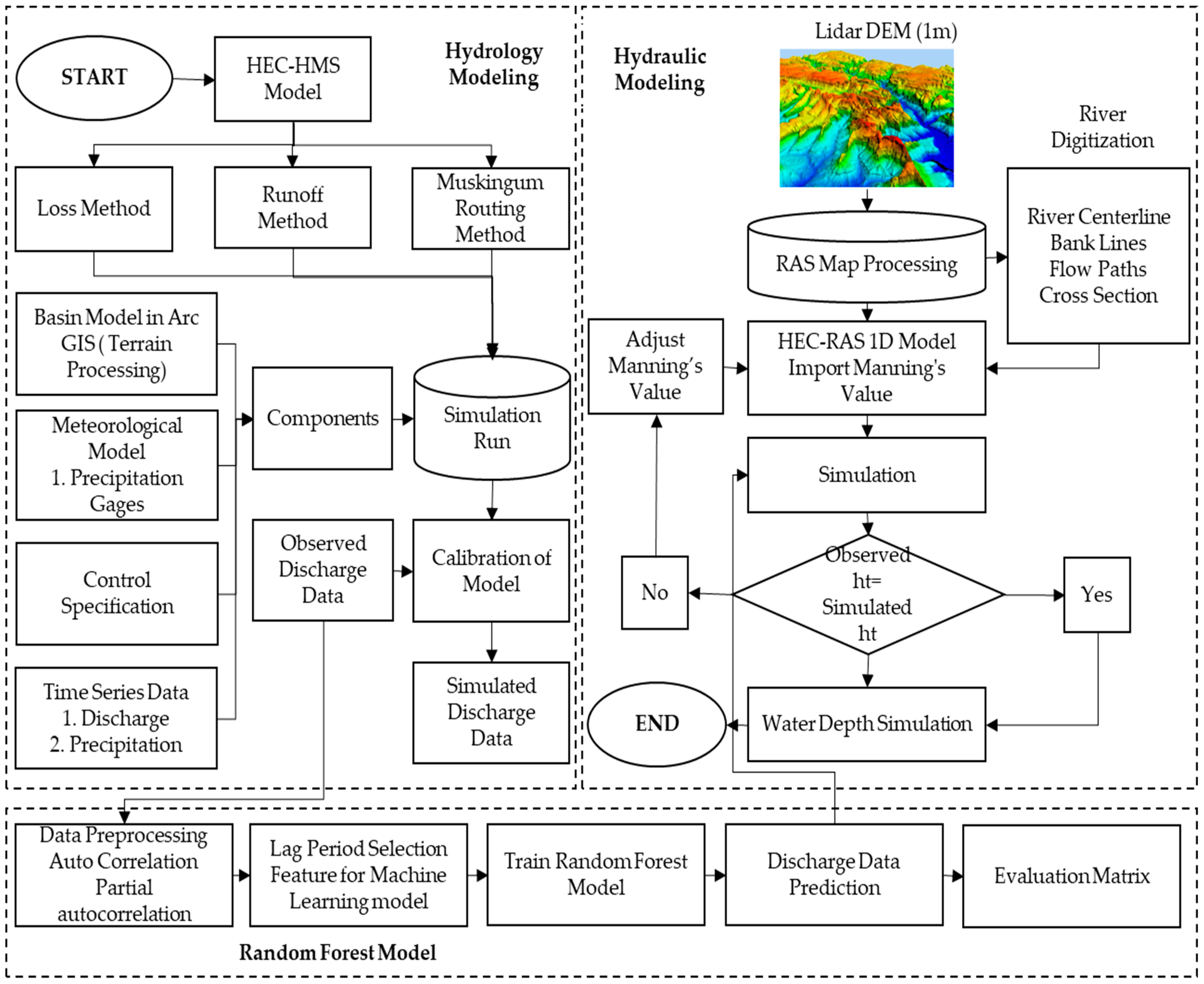
2. Data and Methods
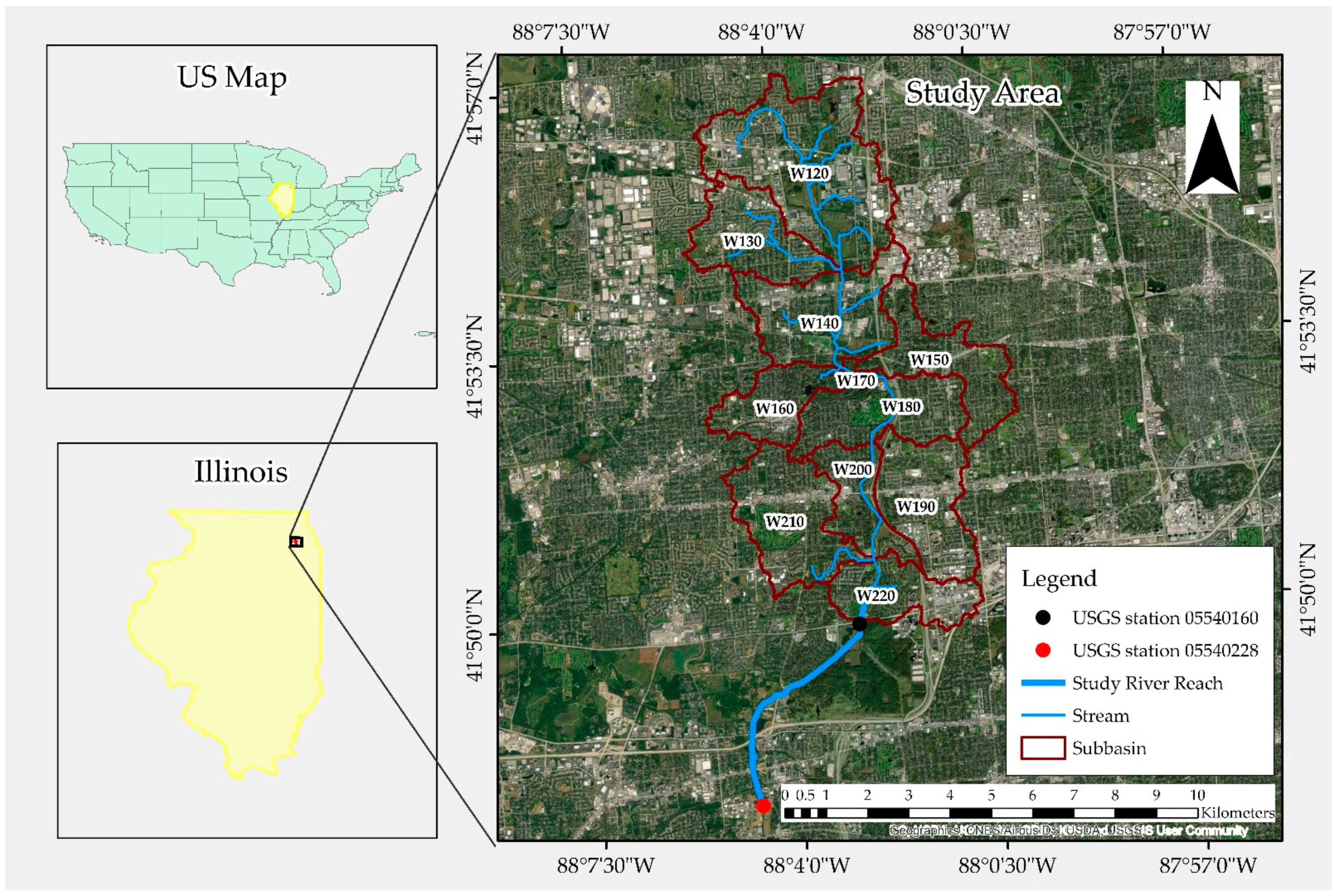
2.1. Study Area
2.2. Data
2.3. Preprocessing Data
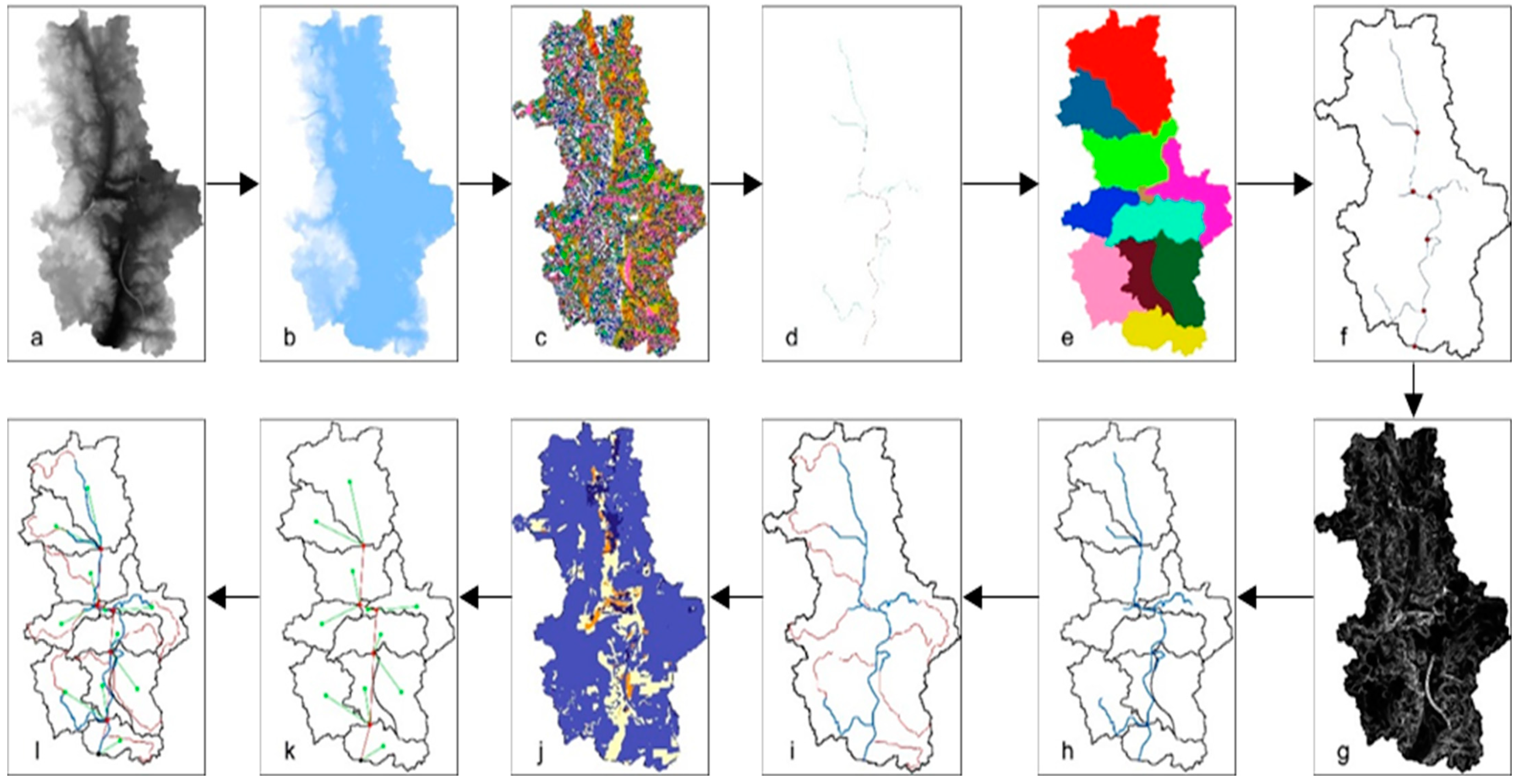
2.3.1. Digital Elevation Model (DEM)
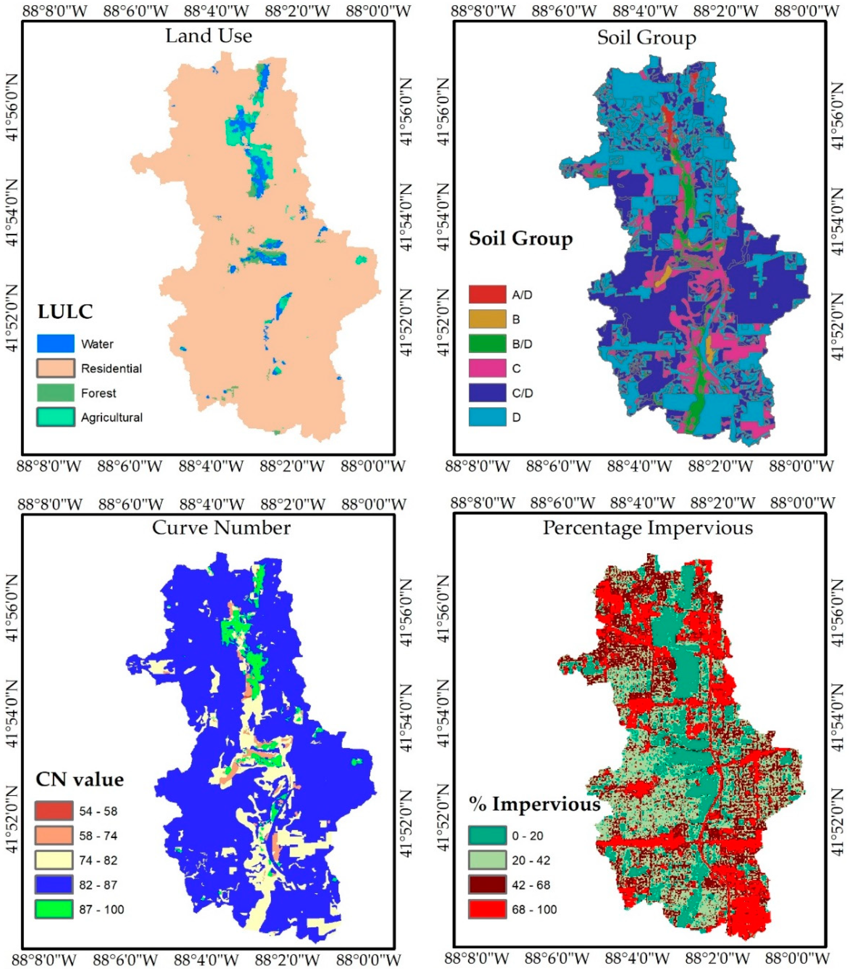
2.3.2. Basin Characteristics
2.3.3. Precipitation Data
2.4. Hydrologic Modeling Using Arc-GIS and HEC-HMS
2.4.1. Loss Method: SCS-CN for Rainfall-Runoff
- Q = Runoff (inches);
- P = Rainfall depth (inches);
- Ia = Initial abstraction, and Ia = 0.2 S;
- S = Potential maximum retention.
2.4.2. Transform Method: SCS Unit Hydrograph
- Tlag = lag time (h);
- L = hydraulic length of the watershed (ft);
- Y = slope of the watershed (%);
- S = maximum retention in the watershed (inches).
2.4.3. Routing Method: Muskingum Routing
2.5. Hydrologic Modeling Using Random Forest
Model Development
2.6. Hydraulic Modeling Using HEC-RAS
- Y1 and Y2 = water heights at cross-sections,
- Z1 and Z2 = elevations of the stream reach,
- α1 and α2 = velocity weighting coefficients,
- V1 and V2 = average velocities,
- g = acceleration due to gravity, and
- he = energy head loss.
River Geometry Generation
2.7. Statistcal Performance Indicators
3. Results and Discussion
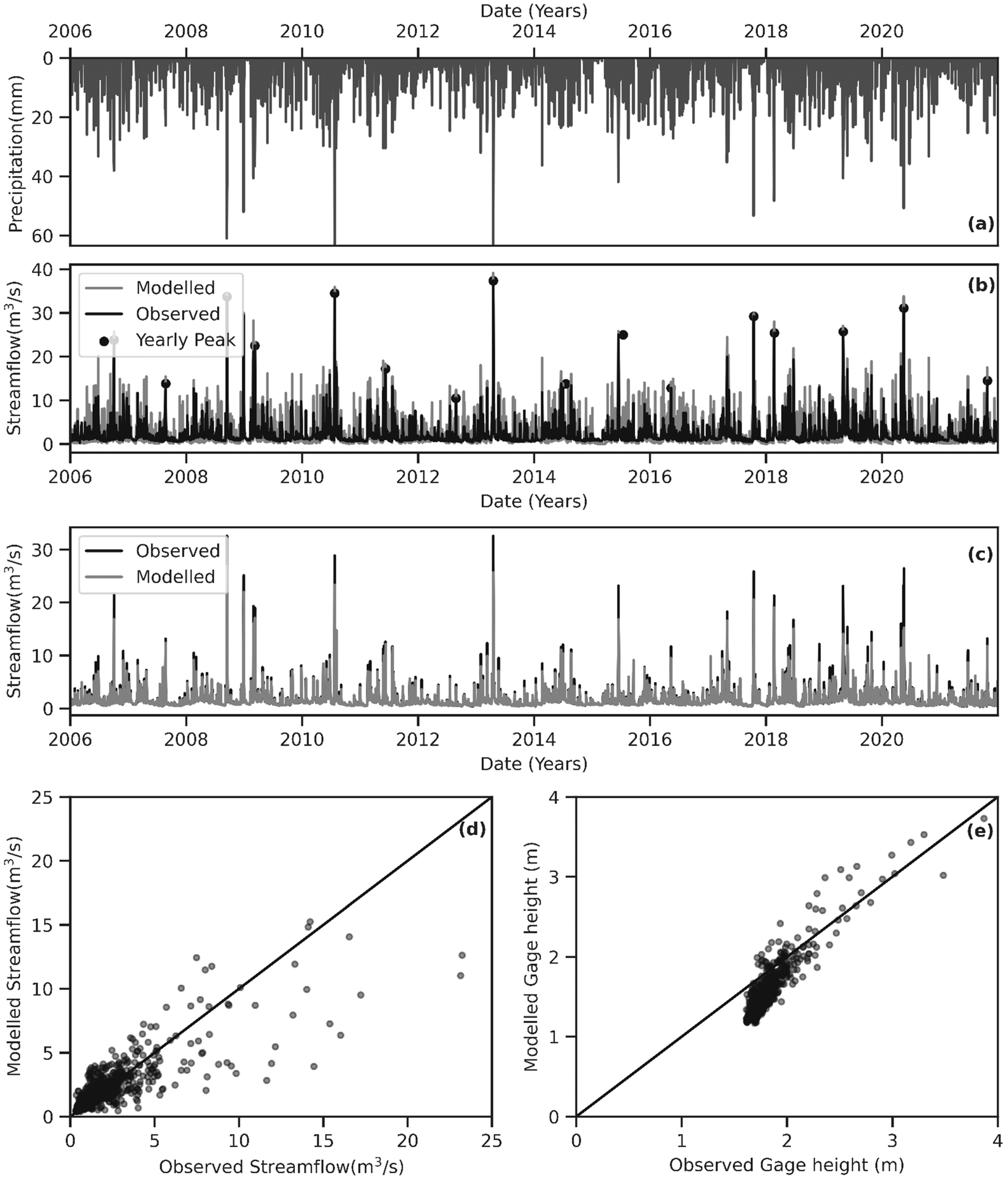
3.1. Precipitation
3.2. HEC-HMS Models
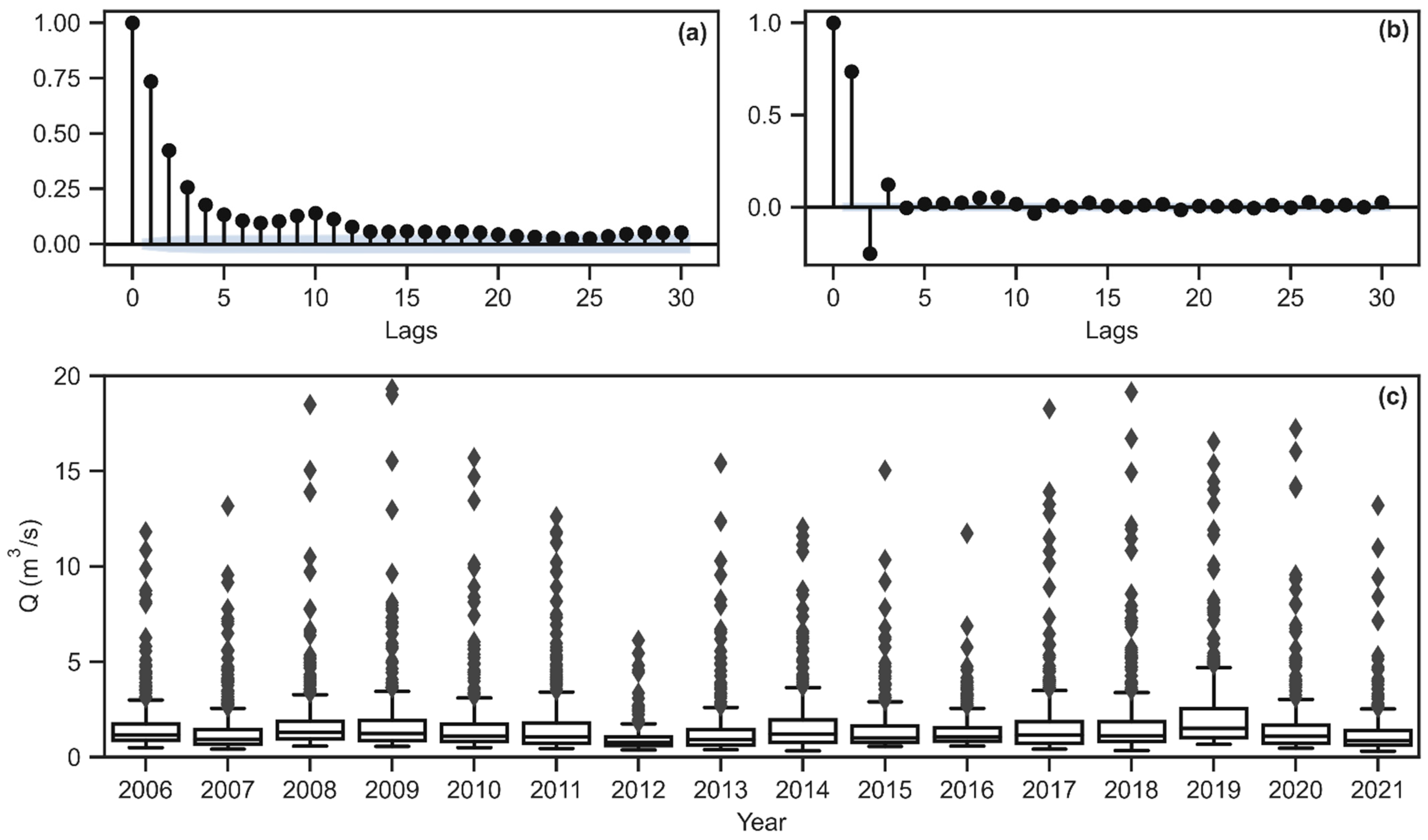
3.3. Random Forest Regression Model
3.4. HEC-RAS Model
4. Discussion
5. Conclusions
- In this study, we used the PERSIANN precipitation product, and future work may be more accurate if there is a precipitation gauging station. Furthermore, researchers could also use other precipitation products, such as Next-Generation Weather Data (NEXRAD) and Climate Hazards Group Infrared Precipitation (CHIRPS);
- In this study, precipitation was only used as an input variable for the Random Forest model; other variables, such as temperature, infiltration, evaporation, and radiation, could be used in future work. In addition, feature selection of input variables could be performed for the most accurate selection;
- Other machine learning and data-driven models, such as support vector regression (SVR), long short-term memory (LSTM), and artificial neural networks (ANNs), could be used as prediction models. Future research directions could be guided by the selection of the best machine learning model in terms of accuracy, robustness, and reliability;
- Although the study area is a small watershed in DuPage County, future research could focus on a more dynamic, heterogeneous, and meteorologically unique basin.
Author Contributions
Funding
Institutional Review Board Statement
Informed Consent Statement
Data Availability Statement
Acknowledgments
Conflicts of Interest
References
- Merwade, V.; Olivera, F.; Arabi, M.; Edleman, S. Uncertainty in Flood Inundation Mapping: Current Issues and Future Directions. J. Hydrol. Eng. 2008, 13, 608–620. [Google Scholar] [CrossRef] [Green Version]
- Merz, B.; Kreibich, H.; Schwarze, R.; Thieken, A. Review Article: Assessment of Economic Flood Damage. Nat. Hazards Earth Syst. Sci. 2010, 10, 1697–1724. [Google Scholar] [CrossRef]
- Gaume, E.; Bain, V.; Bernardara, P.; Newinger, O.; Barbuc, M.; Bateman, A.; Blaškovičová, L.; Blöschl, G.; Borga, M.; Dumitrescu, A.; et al. A Compilation of Data on European Flash Floods. J. Hydrol. 2009, 367, 70–78. [Google Scholar] [CrossRef] [Green Version]
- Ghazali, D.; Guericolas, M.; Thys, F.; Sarasin, F.; Arcos González, P.; Casalino, E. Climate Change Impacts on Disaster and Emergency Medicine Focusing on Mitigation Disruptive Effects: An International Perspective. Int. J. Environ. Res. Public Health 2018, 15, 1379. [Google Scholar] [CrossRef] [PubMed] [Green Version]
- Faccini, F.; Luino, F.; Paliaga, G.; Sacchini, A.; Turconi, L.; de Jong, C. Role of Rainfall Intensity and Urban Sprawl in the 2014 Flash Flood in Genoa City, Bisagno Catchment (Liguria, Italy). Appl. Geogr. 2018, 98, 224–241. [Google Scholar] [CrossRef]
- Sapountzis, M.; Kastridis, A.; Kazamias, A.-P.; Karagiannidis, A.; Nikopoulos, P.; Lagouvardos, K. Utilization and Uncertainties of Satellite Precipitation Data in Flash Flood Hydrological Analysis in Ungauged Watersheds. Glob. NEST J. 2021, 23, 388–399. [Google Scholar] [CrossRef]
- Pathak, P.; Kalra, A.; Ahmad, S. Temperature and Precipitation Changes in the Midwestern United States: Implications for Water Management. Int. J. Water Resour. Dev. 2017, 33, 1003–1019. [Google Scholar] [CrossRef]
- Jenkins, K.; Surminski, S.; Hall, J.; Crick, F. Assessing Surface Water Flood Risk and Management Strategies under Future Climate Change: Insights from an Agent-Based Model. Sci. Total Environ. 2017, 595, 159–168. [Google Scholar] [CrossRef]
- Kundzewicz, Z.W.; Kanae, S.; Seneviratne, S.I.; Handmer, J.; Nicholls, N.; Peduzzi, P.; Mechler, R.; Bouwer, L.M.; Arnell, N.; Mach, K.; et al. Flood Risk and Climate Change: Global and Regional Perspectives. Hydrol. Sci. J. 2014, 59, 1–28. [Google Scholar] [CrossRef] [Green Version]
- Guerreiro, S.B.; Dawson, R.J.; Kilsby, C.; Lewis, E.; Ford, A. Future Heat-Waves, Droughts and Floods in 571 European Cities. Environ. Res. Lett. 2018, 13, 034009. [Google Scholar] [CrossRef]
- Min, S.-K.; Zhang, X.; Zwiers, F.W.; Hegerl, G.C. Human Contribution to More-Intense Precipitation Extremes. Nature 2011, 470, 378–381. [Google Scholar] [CrossRef] [PubMed]
- Vörösmarty, C.J.; de Guenni, L.B.; Wollheim, W.M.; Pellerin, B.; Bjerklie, D.; Cardoso, M.; D’Almeida, C.; Green, P.; Colon, L. Extreme Rainfall, Vulnerability and Risk: A Continental-Scale Assessment for South America. Philos. Trans. R. Soc. A 2013, 371, 20120408. [Google Scholar] [CrossRef] [PubMed]
- Woznicki, S.A.; Baynes, J.; Panlasigui, S.; Mehaffey, M.; Neale, A. Development of a Spatially Complete Floodplain Map of the Conterminous United States Using Random Forest. Sci. Total Environ. 2019, 647, 942–953. [Google Scholar] [CrossRef] [PubMed]
- Archer, D.R.; Fowler, H.J. Characterising Flash Flood Response to Intense Rainfall and Impacts Using Historical Information and Gauged Data in Britain: Flash Flood Response to Intense Rainfall in Britain. J. Flood Risk Manag. 2018, 11, S121–S133. [Google Scholar] [CrossRef]
- Kastridis, A.; Stathis, D. The Effect of Rainfall Intensity on the Flood Generation of Mountainous Watersheds (Chalkidiki Prefecture, North Greece). In Perspectives on Atmospheric Sciences; Karacostas, T., Bais, A., Nastos, P.T., Eds.; Springer Atmospheric Sciences; Springer International Publishing: Cham, Switzerland, 2017; pp. 341–347. ISBN 978-3-319-35094-3. [Google Scholar]
- Schoppa, L.; Disse, M.; Bachmair, S. Evaluating the Performance of Random Forest for Large-Scale Flood Discharge Simulation. J. Hydrol. 2020, 590, 125531. [Google Scholar] [CrossRef]
- Talei, A.; Chua, L.H.C.; Quek, C. A Novel Application of a Neuro-Fuzzy Computational Technique in Event-Based Rainfall–Runoff Modeling. Expert Syst. Appl. 2010, 37, 7456–7468. [Google Scholar] [CrossRef]
- Singh, V.P.; Frevert, D.K. Watershed Models; Taylor and Francis: Abingdon, UK, 2005. [Google Scholar]
- Halwatura, D.; Najim, M.M.M. Application of the HEC-HMS Model for Runoff Simulation in a Tropical Catchment. Environ. Model. Softw. 2013, 46, 155–162. [Google Scholar] [CrossRef]
- US Army Corps of Engineers. Hydrologic Modeling System (HEC-HMS) Application Guide Version 3.1.0; Institute for Water Resources: Davis, CA, USA, 2008. [Google Scholar]
- Bajwa, H.S.; Tim, U.S. Toward Immersive Virtual Environments for GIS-Based Floodplain Modeling and Visualization; ESRI: Redlands, CA, USA, 2002. [Google Scholar]
- Senthil Kumar, A.; Sudheer, K.; Jain, S.; Agarwal, P. Rainfall-runoff modelling using artificial neural networks: Comparison of network types. Hydrol. Process. 2005, 19, 1277–1291. [Google Scholar] [CrossRef]
- Rezaeianzadeh, M.; Stein, A.; Tabari, H.; Abghari, H.; Jalalkamali, N.; Hosseinipour, E.Z.; Singh, V.P. Assessment of a Conceptual Hydrological Model and Artificial Neural Networks for Daily Outflows Forecasting. Int. J. Environ. Sci. Technol. 2013, 10, 1181–1192. [Google Scholar] [CrossRef] [Green Version]
- Kim, B.; Sanders, B.F.; Famiglietti, J.S.; Guinot, V. Urban Flood Modeling with Porous Shallow-Water Equations: A Case Study of Model Errors in the Presence of Anisotropic Porosity. J. Hydrol. 2015, 523, 680–692. [Google Scholar] [CrossRef] [Green Version]
- Sahoo, S.; Russo, T.A.; Elliott, J.; Foster, I. Machine Learning Algorithms for Modeling Groundwater Level Changes in Agricultural Regions of the U.S. Water Resour. Res. 2017, 53, 3878–3895. [Google Scholar] [CrossRef]
- Rajaee, T.; Khani, S.; Ravansalar, M. Artificial Intelligence-Based Single and Hybrid Models for Prediction of Water Quality in Rivers: A Review. Chemom. Intell. Lab. Syst. 2020, 200, 103978. [Google Scholar] [CrossRef]
- Zounemat-Kermani, M.; Batelaan, O.; Fadaee, M.; Hinkelmann, R. Ensemble Machine Learning Paradigms in Hydrology: A Review. J. Hydrol. 2021, 598, 126266. [Google Scholar] [CrossRef]
- Jordan, M.I.; Mitchell, T.M. Machine Learning: Trends, Perspectives, and Prospects. Science 2015, 349, 255–260. [Google Scholar] [CrossRef] [PubMed]
- Ghimire, S.; Yaseen, Z.M.; Farooque, A.A.; Deo, R.C.; Zhang, J.; Tao, X. OPEN Streamflow Prediction Using. Sci. Rep. 2021, 11, 17497. [Google Scholar] [CrossRef]
- Mewes, B.; Oppel, H.; Marx, V.; Hartmann, A. Information-Based Machine Learning for Tracer Signature Prediction in Karstic Environments. Water Resour. Res. 2020, 56, e2018WR024558. [Google Scholar] [CrossRef]
- Parisouj, P.; Mohebzadeh, H.; Lee, T. Employing Machine Learning Algorithms for Streamflow Prediction: A Case Study of Four River Basins with Different Climatic Zones in the United States. Water Resour. Manag. 2020, 34, 4113–4131. [Google Scholar] [CrossRef]
- Adnan, R.M.; Petroselli, A.; Heddam, S.; Santos, C.A.G.; Kisi, O. Short Term Rainfall-Runoff Modelling Using Several Machine Learning Methods and a Conceptual Event-Based Model. Stoch. Environ. Res. Risk Assess. 2021, 35, 597–616. [Google Scholar] [CrossRef]
- Shamshirband, S.; Hashemi, S.; Salimi, H.; Samadianfard, S.; Asadi, E.; Shadkani, S.; Kargar, K.; Mosavi, A.; Nabipour, N.; Chau, K.-W. Predicting Standardized Streamflow Index for Hydrological Drought Using Machine Learning Models. Eng. Appl. Comput. Fluid Mech. 2020, 14, 339–350. [Google Scholar] [CrossRef]
- Nguyen, D.T.; Chen, S.-T. Real-Time Probabilistic Flood Forecasting Using Multiple Machine Learning Methods. Water 2020, 12, 787. [Google Scholar] [CrossRef] [Green Version]
- Zhou, Y.; Cui, Z.; Lin, K.; Sheng, S.; Chen, H.; Guo, S.; Xu, C.-Y. Short-Term Flood Probability Density Forecasting Using a Conceptual Hydrological Model with Machine Learning Techniques. J. Hydrol. 2022, 604, 127255. [Google Scholar] [CrossRef]
- Kalra, A.; Ahmad, S.; Nayak, A. Increasing Streamflow Forecast Lead Time for Snowmelt-Driven Catchment Based on Large-Scale Climate Patterns. Adv. Water Resour. 2013, 53, 150–162. [Google Scholar] [CrossRef]
- Rezaei, K.; Pradhan, B.; Vadiati, M.; Nadiri, A.A. Suspended Sediment Load Prediction Using Artificial Intelligence Techniques: Comparison between Four State-of-the-Art Artificial Neural Network Techniques. Arab. J. Geosci. 2021, 14, 215. [Google Scholar] [CrossRef]
- Choubin, B.; Darabi, H.; Rahmati, O.; Sajedi-Hosseini, F.; Kløve, B. River Suspended Sediment Modelling Using the CART Model: A Comparative Study of Machine Learning Techniques. Sci. Total Environ. 2018, 615, 272–281. [Google Scholar] [CrossRef] [PubMed]
- Rezaei, K.; Vadiati, M. A Comparative Study of Artificial Intelligence Models for Predicting Monthly River Suspended Sediment Load. J. Water Land Dev. 2020, 45, 107–118. [Google Scholar] [CrossRef]
- Wang, S.; Peng, H.; Liang, S. Prediction of Estuarine Water Quality Using Interpretable Machine Learning Approach. J. Hydrol. 2022, 605, 127320. [Google Scholar] [CrossRef]
- Deng, T.; Chau, K.-W.; Duan, H.-F. Machine Learning Based Marine Water Quality Prediction for Coastal Hydro-Environment Management. J. Environ. Manag. 2021, 284, 112051. [Google Scholar] [CrossRef]
- Melesse, A.M.; Khosravi, K.; Tiefenbacher, J.P.; Heddam, S.; Kim, S.; Mosavi, A.; Pham, B.T. River Water Salinity Prediction Using Hybrid Machine Learning Models. Water 2020, 12, 2951. [Google Scholar] [CrossRef]
- Asadollah, S.B.H.S.; Sharafati, A.; Motta, D.; Yaseen, Z.M. River Water Quality Index Prediction and Uncertainty Analysis: A Comparative Study of Machine Learning Models. J. Environ. Chem. Eng. 2021, 9, 104599. [Google Scholar] [CrossRef]
- Hussein, E.A.; Thron, C.; Ghaziasgar, M.; Bagula, A.; Vaccari, M. Groundwater Prediction Using Machine-Learning Tools. Algorithms 2020, 13, 300. [Google Scholar] [CrossRef]
- Khedri, A.; Kalantari, N.; Vadiati, M. Comparison Study of Artificial Intelligence Method for Short Term Groundwater Level Prediction in the Northeast Gachsaran Unconfined Aquifer. Water Supply 2020, 20, 909–921. [Google Scholar] [CrossRef]
- Zhu, S.; Piotrowski, A.P. River/Stream Water Temperature Forecasting Using Artificial Intelligence Models: A Systematic Review. Acta Geophys. 2020, 68, 1433–1442. [Google Scholar] [CrossRef]
- Chang, H.; Psaris, M. Local Landscape Predictors of Maximum Stream Temperature and Thermal Sensitivity in the Columbia River Basin, USA. Sci. Total Environ. 2013, 461–462, 587–600. [Google Scholar] [CrossRef] [PubMed]
- Weierbach, H.; Lima, A.R.; Willard, J.D.; Hendrix, V.C.; Christianson, D.S.; Lubich, M.; Varadharajan, C. Stream Temperature Predictions for River Basin Management in the Pacific Northwest and Mid-Atlantic Regions Using Machine Learning. Water 2022, 14, 1032. [Google Scholar] [CrossRef]
- Feigl, M.; Lebiedzinski, K.; Herrnegger, M.; Schulz, K. Machine-learning methods for stream water temperature prediction. Hydrol. Earth Syst. Sci. 2021, 25, 2951–2977. [Google Scholar] [CrossRef]
- Zhang, J.; Xu, J.; Dai, X.; Ruan, H.; Liu, X.; Jing, W. Multi-Source Precipitation Data Merging for Heavy Rainfall Events Based on Cokriging and Machine Learning Methods. Remote Sens. 2022, 14, 1750. [Google Scholar] [CrossRef]
- Radhakrishnan, C.; Chandrasekar, V.; Reising, S.C.; Berg, W. Rainfall Estimation from TEMPEST-D CubeSat Observations: A Machine-Learning Approach. IEEE J. Sel. Top. Appl. Earth Obs. Remote Sens. 2022, 15, 3626–3636. [Google Scholar] [CrossRef]
- Guo, W.-D.; Chen, W.-B.; Yeh, S.-H.; Chang, C.-H.; Chen, H. Prediction of River Stage Using Multistep-Ahead Machine Learning Techniques for a Tidal River of Taiwan. Water 2021, 13, 920. [Google Scholar] [CrossRef]
- Chiang, S.; Chang, C.-H.; Chen, W.-B. Comparison of Rainfall-Runoff Simulation between Support Vector Regression and HEC-HMS for a Rural Watershed in Taiwan. Water 2022, 14, 191. [Google Scholar] [CrossRef]
- Ni, L.; Wang, D.; Singh, V.P.; Wu, J.; Wang, Y.; Tao, Y.; Zhang, J. Streamflow and Rainfall Forecasting by Two Long Short-Term Memory-Based Models. J. Hydrol. 2020, 583, 124296. [Google Scholar] [CrossRef]
- Yin, H.; Wang, F.; Zhang, X.; Zhang, Y.; Chen, J.; Xia, R.; Jin, J. Rainfall-Runoff Modeling Using Long Short-Term Memory Based Step-Sequence Framework. J. Hydrol. 2022, 610, 127901. [Google Scholar] [CrossRef]
- Tikhamarine, Y.; Souag-Gamane, D.; Ahmed, A.N.; Sammen, S.S.; Kisi, O.; Huang, Y.F.; El-Shafie, A. Rainfall-Runoff Modelling Using Improved Machine Learning Methods: Harris Hawks Optimizer vs. Particle Swarm Optimization. J. Hydrol. 2020, 589, 125133. [Google Scholar] [CrossRef]
- Tamiru, H.; Dinka, M.O. Application of ANN and HEC-RAS Model for Flood Inundation Mapping in Lower Baro Akobo River Basin, Ethiopia. J. Hydrol. Reg. Stud. 2021, 36, 100855. [Google Scholar] [CrossRef]
- Samantaray, S.; Das, S.S.; Sahoo, A.; Satapathy, D.P. Monthly Runoff Prediction at Baitarani River Basin by Support Vector Machine Based on Salp Swarm Algorithm. Ain Shams Eng. J. 2022, 13, 101732. [Google Scholar] [CrossRef]
- Adnan, R.M.; Liang, Z.; Heddam, S.; Zounemat-Kermani, M.; Kisi, O.; Li, B. Least Square Support Vector Machine and Multivariate Adaptive Regression Splines for Streamflow Prediction in Mountainous Basin Using Hydro-Meteorological Data as Inputs. J. Hydrol. 2020, 586, 124371. [Google Scholar] [CrossRef]
- Worland, S.C.; Farmer, W.H.; Kiang, J.E. Improving Predictions of Hydrological Low-Flow Indices in Ungaged Basins Using Machine Learning. Environ. Model. Softw. 2018, 101, 169–182. [Google Scholar] [CrossRef]
- Breiman, L. Random Forests. Mach. Learn. 2001, 45, 5–32. [Google Scholar] [CrossRef] [Green Version]
- Zhou, P.; Li, Z.; Snowling, S.; Baetz, B.W.; Na, D.; Boyd, G. A Random Forest Model for Inflow Prediction at Wastewater Treatment Plants. Stoch. Environ. Res. Risk Assess. 2019, 33, 1781–1792. [Google Scholar] [CrossRef]
- Meng, Y.; Yang, M.; Liu, S.; Mou, Y.; Peng, C.; Zhou, X. Quantitative Assessment of the Importance of Bio-Physical Drivers of Land Cover Change Based on a Random Forest Method. Ecol. Inform. 2021, 61, 101204. [Google Scholar] [CrossRef]
- Li, B.; Yang, G.; Wan, R.; Dai, X.; Zhang, Y. Comparison of Random Forests and Other Statistical Methods for the Prediction of Lake Water Level: A Case Study of the Poyang Lake in China. Hydrol. Res. 2016, 47, 69–83. [Google Scholar] [CrossRef] [Green Version]
- Bachmair, S.; Svensson, C.; Prosdocimi, I.; Hannaford, J.; Stahl, K. Developing Drought Impact Functions for Drought Risk Management. Nat. Hazards Earth Syst. Sci. 2017, 17, 1947–1960. [Google Scholar] [CrossRef] [Green Version]
- Erdal, H.I.; Karakurt, O. Advancing Monthly Streamflow Prediction Accuracy of CART Models Using Ensemble Learning Paradigms. J. Hydrol. 2013, 477, 119–128. [Google Scholar] [CrossRef]
- Muñoz, P.; Orellana-Alvear, J.; Willems, P.; Célleri, R. Flash-Flood Forecasting in an Andean Mountain Catchment—Development of a Step-Wise Methodology Based on the Random Forest Algorithm. Water 2018, 10, 1519. [Google Scholar] [CrossRef] [Green Version]
- Tyralis, H.; Papacharalampous, G.; Langousis, A. A Brief Review of Random Forests for Water Scientists and Practitioners and Their Recent History in Water Resources. Water 2019, 11, 910. [Google Scholar] [CrossRef] [Green Version]
- Wang, Z.; Lai, C.; Chen, X.; Yang, B.; Zhao, S.; Bai, X. Flood Hazard Risk Assessment Model Based on Random Forest. J. Hydrol. 2015, 527, 1130–1141. [Google Scholar] [CrossRef]
- Feng, Q.; Liu, J.; Gong, J. Urban Flood Mapping Based on Unmanned Aerial Vehicle Remote Sensing and Random Forest Classifier—A Case of Yuyao, China. Water 2015, 7, 1437–1455. [Google Scholar] [CrossRef]
- Quirogaa, V.M.; Kurea, S.; Udoa, K.; Manoa, A. Application of 2D Numerical Simulation for the Analysis of the February 2014 Bolivian Amazonia Flood: Application of the New HEC-RAS Version 5. Ribagua 2016, 3, 25–33. [Google Scholar] [CrossRef] [Green Version]
- Brunner, G. HEC-RAS, River Analysis System Hydraulic Reference Manual; U.S. Army Corps of Engineers: Davis, CA, USA, 2016. [Google Scholar]
- İcaga, Y.; Tas, E.; Kilit, M. Flood Inundation Mapping by GIS and a Hydraulic Model (Hec Ras): A Case Study of Akarcay Bolvadin Subbasin, in Turkey. Acta Geobalcanica 2016, 2, 111–118. [Google Scholar] [CrossRef]
- Abaya, S.W.; Mandere, N.; Ewald, G. Floods and Health in Gambella Region, Ethiopia: A Qualitative Assessment of the Strengths and Weaknesses of Coping Mechanisms. Glob. Health Action 2009, 2, 2019. [Google Scholar] [CrossRef] [Green Version]
- US Army Corps of Engineers. Dupage River, Illinois Feasibility Report and Integrated Environmental Assessment; US Army Corps of Engineers: Chicago, IL, USA, 2019. [Google Scholar]
- StreamStats. Available online: https://Streamstats.Usgs.Gov/Ss/ (accessed on 15 June 2022).
- Nguyen, P.; Shearer, E.J.; Tran, H.; Ombadi, M.; Hayatbini, N.; Palacios, T.; Huynh, P.; Braithwaite, D.; Updegraff, G.; Hsu, K.; et al. The CHRS Data Portal, an Easily Accessible Public Repository for PERSIANN Global Satellite Precipitation Data. Sci. Data 2019, 6, 180296. [Google Scholar] [CrossRef] [Green Version]
- Mockus, V. National Engineering Handbook Section 4 HydrologY; US Soil Conservation Service: Washington, DC, USA, 1972; p. 127.
- Saadi, M.; Oudin, L.; Ribstein, P. Random Forest Ability in Regionalizing Hourly Hydrological Model Parameters. Water 2019, 11, 1540. [Google Scholar] [CrossRef] [Green Version]
- Müller, A.; Guido, S. Introduction to Machine Learning with Python: A Guide for Data Scientists, 1st ed.; O’Reilly: Farnham, UK, 2016. [Google Scholar]
- Park, H.; Kim, K.; Lee, D.K. Prediction of Severe Drought Area Based on Random Forest: Using Satellite Image and Topography Data. Water 2019, 11, 705. [Google Scholar] [CrossRef] [Green Version]
- Biau, G.; Scornet, E. A Random Forest Guided Tour. Test 2016, 25, 197–227. [Google Scholar] [CrossRef] [Green Version]
- Gregorutti, B.; Michel, B.; Saint-Pierre, P. Correlation and Variable Importance in Random Forests. Stat. Comput. 2017, 27, 659–678. [Google Scholar] [CrossRef] [Green Version]
- Hussain, D.; Khan, A.A. Machine Learning Techniques for Monthly River Flow Forecasting of Hunza River, Pakistan. Earth Sci. Inf. 2020, 13, 939–949. [Google Scholar] [CrossRef]
- Gharbi, M.; Soualmia, A.; Dartus, D.; Masbernat, L. Comparison of 1D and 2D Hydraulic Models for Floods Simulation on the Medjerda Riverin Tunisia. J. Mater. Environ. Sci. 2016, 7, 3017–3026. [Google Scholar]
- Pathan, A.I.; Agnihotri, P.G. Application of New HEC-RAS Version 5 for 1D Hydrodynamic Flood Modeling with Special Reference through Geospatial Techniques: A Case of River Purna at Navsari, Gujarat, India. Model. Earth Syst. Environ. 2021, 7, 1133–1144. [Google Scholar] [CrossRef]
- Hydrologic and Water Quality Models: Performance Measures and Evaluation Criteria. Trans. ASABE 2015, 58, 1763–1785. [CrossRef] [Green Version]
- Kumar, N.; Singh, S.K.; Srivastava, P.K.; Narsimlu, B. SWAT Model Calibration and Uncertainty Analysis for Streamflow Prediction of the Tons River Basin, India, Using Sequential Uncertainty Fitting (SUFI-2) Algorithm. Model. Earth Syst. Environ. 2017, 3, 30. [Google Scholar] [CrossRef]
- Abbaspour, K.C.; Rouholahnejad, E.; Vaghefi, S.; Srinivasan, R.; Yang, H.; Kløve, B. A Continental-Scale Hydrology and Water Quality Model for Europe: Calibration and Uncertainty of a High-Resolution Large-Scale SWAT Model. J. Hydrol. 2015, 524, 733–752. [Google Scholar] [CrossRef] [Green Version]
- Gupta, H.V.; Sorooshian, S.; Yapo, P.O. Status of Automatic Calibration for Hydrologic Models: Comparison with Multilevel Expert Calibration. J. Hydrol. Eng. 1999, 4, 135–143. [Google Scholar] [CrossRef]
- Hong, Y.; Gochis, D.; Cheng, J.; Hsu, K.; Sorooshian, S. Evaluation of PERSIANN-CCS Rainfall Measurement Using the NAME Event Rain Gauge Network. J. Hydrometeorol. 2007, 8, 469–482. [Google Scholar] [CrossRef] [Green Version]
- Joshi, N.; Bista, A.; Pokhrel, I.; Kalra, A.; Ahmad, S. Rainfall-Runoff Simulation in Cache River Basin, Illinois, Using HEC-HMS. In World Environmental and Water Resources Congress 2019; American Society of Civil Engineers: Pittsburgh, PA, USA, 2019; pp. 348–360. [Google Scholar]
- Desai, S.; Ouarda, T.B.M.J. Regional Hydrological Frequency Analysis at Ungauged Sites with Random Forest Regression. J. Hydrol. 2021, 594, 125861. [Google Scholar] [CrossRef]


| Data | Source |
|---|---|
| Precipitation | Precipitation Estimation from Remotely Sensed Information Using Artificial Neural Networks–Cloud Classification System (PERSIANN-CCS). |
| Soil | United States Department of Agriculture (USDA) |
| Land Use Land Cover | United States Geological Survey (USGS) |
| Runoff Data | United States Geological Survey (USGS) water data |
| Lag (Days) | The Structure of the Input | Output |
|---|---|---|
| 5 | Discharge of 1 day to the 5-day lag period, Precipitation of 1 day to the 5-day lag period, Sum of 5 days of precipitation (P5 days), Days since last precipitation greater than 0.5 mm. (p > 0.5) | One day ahead discharge |
| Indices | Mathematical Expression | Satisfactory Range |
|---|---|---|
| Root Mean Square Error (RMSE) | ||
| Nash–Sutcliffe efficiency coefficient (NSE) | 0.5 < NSE ≤ 1 | |
| Coefficient of Determination (R2) | >0.5 | |
| Standard Deviation Ratio (RSR) | 0 < RSR < 0.7 | |
| Percentage bias (PBIAS) | −25% < PBIAS < +25% | |
| Normalized Root Mean Squared Error (NRMSE) | ≤30% |
| Sub-Basin | Basin Area (km2) | Basin Slope (%) | Curve Number (CN) | Basin Lag (min) |
|---|---|---|---|---|
| W220 | 4.3 | 2.6 | 85.8 | 150 |
| W210 | 7.0 | 2.8 | 84.7 | 135 |
| W200 | 3.6 | 3.1 | 83.6 | 133 |
| W190 | 6.2 | 1.9 | 83.9 | 84 |
| W180 | 5.9 | 3.5 | 83.2 | 90 |
| W170 | 0.3 | 4.5 | 86.7 | 84 |
| W160 | 3.7 | 2.6 | 82.3 | 81 |
| W150 | 5.5 | 3.5 | 83.7 | 98 |
| W140 | 7.4 | 4.5 | 83.0 | 86 |
| W130 | 5.3 | 2.2 | 84.2 | 20 |
| W120 | 13.0 | 3.4 | 84.0 | 76 |
| Statistical Index | HEC-HMS Model | Random Forest | ||
|---|---|---|---|---|
| Calibration | Validation | Training | Testing | |
| RMSE (m3/s) | 1.45 | 2.45 | 0.29 | 0.47 |
| RSR | 0.16 | 0.35 | 0.23 | 0.56 |
| NSE | 0.97 | 0.87 | 0.94 | 0.69 |
| PBIAS | −5.30% | −9.80% | −0.75% | +1.76% |
| R2 | 0.99 | 0.96 | 0.94 | 0.72 |
| NRMSE | 0.06 | 0.10 | 0.17 | 0.26 |
| Event | Discharge (m3/s) | Observed Water Depth (m) | Simulated Water Depth (m) | Difference (m) |
|---|---|---|---|---|
| 11 January 2020 | 8.78 | 2.79 | 2.68 | 0.11 |
| 30 March 2020 | 3.11 | 2.09 | 1.98 | 0.11 |
| 29 March 2020 | 5.07 | 2.33 | 2.58 | −0.25 |
| 30 April 2020 | 16.03 | 3.40 | 3.02 | 0.38 |
| 18 May 2020 | 26.42 | 4.41 | 3.85 | 0.56 |
| 23 October 2020 | 6.57 | 2.45 | 2.91 | −0.46 |
| 12 December 2020 | 8.04 | 2.52 | 2.61 | −0.09 |
| 19 March 2021 | 2.83 | 1.96 | 2.03 | −0.07 |
| 26 June 2021 | 10.96 | 2.90 | 3.27 | −0.37 |
| 27 August 2021 | 2.21 | 1.81 | 1.89 | −0.08 |
| 26 October 2021 | 8.38 | 2.50 | 2.48 | 0.02 |
Publisher’s Note: MDPI stays neutral with regard to jurisdictional claims in published maps and institutional affiliations. |
© 2022 by the authors. Licensee MDPI, Basel, Switzerland. This article is an open access article distributed under the terms and conditions of the Creative Commons Attribution (CC BY) license (https://creativecommons.org/licenses/by/4.0/).
Share and Cite
Bhusal, A.; Parajuli, U.; Regmi, S.; Kalra, A. Application of Machine Learning and Process-Based Models for Rainfall-Runoff Simulation in DuPage River Basin, Illinois. Hydrology 2022, 9, 117. https://0-doi-org.brum.beds.ac.uk/10.3390/hydrology9070117
Bhusal A, Parajuli U, Regmi S, Kalra A. Application of Machine Learning and Process-Based Models for Rainfall-Runoff Simulation in DuPage River Basin, Illinois. Hydrology. 2022; 9(7):117. https://0-doi-org.brum.beds.ac.uk/10.3390/hydrology9070117
Chicago/Turabian StyleBhusal, Amrit, Utsav Parajuli, Sushmita Regmi, and Ajay Kalra. 2022. "Application of Machine Learning and Process-Based Models for Rainfall-Runoff Simulation in DuPage River Basin, Illinois" Hydrology 9, no. 7: 117. https://0-doi-org.brum.beds.ac.uk/10.3390/hydrology9070117