T4SS Effector Protein Prediction with Deep Learning


1
Department of Computer Engineering, Baskent University, Bağlıca Kampüsü Fatih Sultan Mahallesi Eskişehir Yolu 18.km, Ankara 06709, Turkey
2
Faculty of Computer Science, Østfold University College, P.O. Box 700, 1757 Halden, Norway
*
Author to whom correspondence should be addressed.
Data 2019, 4(1), 45; https://0-doi-org.brum.beds.ac.uk/10.3390/data4010045
Submission received: 1 February 2019
/
Revised: 19 March 2019
/
Accepted: 22 March 2019
/
Published: 25 March 2019
Abstract
:Extensive research has been carried out on bacterial secretion systems, as they can pass effector proteins directly into the cytoplasm of host cells. The correct prediction of type IV protein effectors secreted by T4SS is important, since they are known to play a noteworthy role in various human pathogens. Studies on predicting T4SS effectors involve traditional machine learning algorithms. In this work we included a deep learning architecture, i.e., a Convolutional Neural Network (CNN), to predict IVA and IVB effectors. Three feature extraction methods were utilized to represent each protein as an image and these images fed the CNN as inputs in our proposed framework. Pseudo proteins were generated using ADASYN algorithm to overcome the imbalanced dataset problem. We demonstrated that our framework predicted all IVA effectors correctly. In addition, the sensitivity performance of 94.2% for IVB effector prediction exhibited our framework’s ability to discern the effectors in unidentified proteins.
1. Introduction
Effector proteins are generally critical for bacterial virulence. They are excreted by various pathogens into host cells through secretion systems. Type IV secretion system (T4SS) is one of the seven secretion systems in gram-negative bacteria and capable of transporting both proteins and nucleoprotein complexes (protein–protein and protein–DNA) [1,2]. This ability makes it unique among other bacterial secretion systems [3]. By using T4SS, effector proteins can be transported into the cytoplasm of a host cell directly, across the bacterial membrane and the plasmatic membrane of eukaryotic host cell. This process results in several diseases. For example, Helicobacter pylori uses a T4SS (Cag) to deliver CagA (cytotoxin-associated gene A) into gastric epithelial cells, which causes gastritis and peptic ulcer [4]. Bordetella pertussis secretes the pertussis toxin through a T4SS (pertussis toxin liberation (Ptl)), which causes whooping cough (i.e., pertussis), a contagious bacterial infection of the lungs and airways [5]. Legionella pneumophila, which causes legionellosis (Legionnaires’ disease), utilizes a T4SS known as Dot/Icm (defect in organelle trafficking genes/intracellular multiplication) to transmit numerous effector proteins into its eukaryotic host [6]. Agrobacterium tumefaciens uses VirB T4SS and causes a crown gall (tumor) in plant host [7]. Bartonella spp. exploits VirB and Trw T4SSs and effector translocation results in cat-scratch disease and angiomatosis [8,9]. Brucella spp. utilizes VirB T4SS and causes a bacterial infection called brucellosis that spreads from animals to people via unpasteurized milk or undercooked meat [10].
There are two different classification schemes for T4SSs [11,12]. In the original one, there are three major types (classes) called as F, P and I. In the alternative one, types F and P are grouped together and called type IVA while the remaining type I is called type IVB. Additionally, a third group that has a great genetic distance from the other types is identified and named as type GI [13]. Thus, prediction of proteins that belong to the same secretion system from different types has become important.
Effector protein prediction has a very important place in biology because it defines the pathogens that effecting cells [3]. Therefore, prediction of these proteins is crucial to find the pathogens and identify them. Prediction of effector proteins that are secreted by secretion systems is experimentally time-consuming and expensive. Therefore, various computational methods have emerged. Machine learning algorithms are widely used to predict T4SS effector proteins.
Burstein et al. [14] studied Legionella pneumophila to distinguish T4SS effectors from non-effectors and validate new effectors. They extracted seven features, namely sequence similarity to known effectors and eukaryotic proteomes, taxonomic distribution, genome organization, G + C content, C-terminal signal and regulatory elements, to feed machine learning algorithms. In addition, they combined all features to increase the classification performance. For classification tests, they took advantage of Naïve Bayes (NB), Support Vector Machines (SVM) and Neural Networks (MLP or NN). Finally, they applied a voting scheme that considers these three machine learning algorithms. During the evaluation of classification performance, they used a dataset with a ratio of 1:1 of effectors and non-effectors. As a result, using taxonomic distribution features outperforms others in terms of correct rate and Area Under Curve (AUC) measures, but the best performance is achieved by combining all features. Another success of the study is the prediction and validation of 40 novel effectors.
Zou et al. [15] worked on predicting T4SS effectors from different species. They divided T4SS effectors as IVA and IVB effectors. Amino acid composition (AAC), dipeptide composition (DPC), position specific scoring matrix composition (PSSM), auto covariance transformation of PSSM (PSSM_AC) and several combinations of them are used as feature vectors in classification tasks. The features are extracted using primary sequence structure of proteins. They chose SVM classifier to predict whether the test protein is an effector. Leave-one-out tests are implemented on a dataset with a ratio of 1:4 of IVA and IVB effectors. According to experiments, some of the combined feature vectors have better results than the single ones. Additionally, four SVMs, fed by four different features, are organized to predict an unknown protein based on majority voting scheme. They found that an ensemble classifier using AAC, PSSM and PSSM_AC features has higher performance rates in terms of sensitivity, specificity, accuracy and MCC.
Wang et al. [16] began their research by identifying the lack of an inter-species tool for predicting T4SS effectors. C-terminal sequential and position-specific amino acid compositions, secondary structure, tertiary structure and solvent accessibility information from various bacteria are used for feeding the SVM classifier. Several models, based on the features, are set up to predict T4SS effectors on a dataset with a ratio of 1:6 of effectors and non-effectors. A model called T4SEpre_Joint (trained by using position specific amino acid compositions, secondary structures and solvent accessibility values) by the authors gives the best performance results. The most remarkable aspect of the study is the identification of 24 candidate Helicobacter pylori effectors.
Zou and Chen [17] analyzed C-terminal sequence features and used them to predict type IVB effectors based on several machine learning algorithms including NB, SVM, RBF neural network, SMO and Hoeffding Tree as well as majority voting. To feed the classifiers C-terminal sequence features and position-specific amino acid composition features are extracted. They used a dataset with a ratio of 1:3. The best performance results, in terms of sensitivity, specificity, accuracy, MCC and Ppv, asre obtained by running tests on SVM and combining both extracted features. The main contribution of the research is that the proposed method is sensitive to predict IVB effectors in Coxiella burnetii.
Wang et al. [18] developed an ensemble classifier including NB, kNN, Logistic Regression (LR), Random Forest (RF), MLP and SVM. This ensemble classifier is called Bastion4 and serves as an online T4SS effector predictor. They used 10 types of feature vectors to feed the classifiers. Final prediction result of a query protein is given after majority voting process based on the six classifiers. According to their main findings, RF and SVM outperforms other classifiers in terms of accuracy, F-value and MCC; the best performance values are obtained when PSSM feature vector is used as input for all classifiers; combining features increases performance results and majority voting strategy gives more stable and accurate prediction performance for T4SS effectors. Additionally, they compared their model with current T4SS predictors [15,16] and revealed that Bastion4 outperforms all of them.
All published studies on predicting T4SS effectors use traditional machine learning algorithms. To our knowledge, a deep learning method has not yet been used to predict T4SS effector proteins. We propose a framework that uses a convolutional neural network for classification. To feed the CNN, all proteins were converted into RGB images according to their amino acid compositions, dipeptide compositions and position-specific scoring matrix representations.
2. Methods
2.1. General Framework
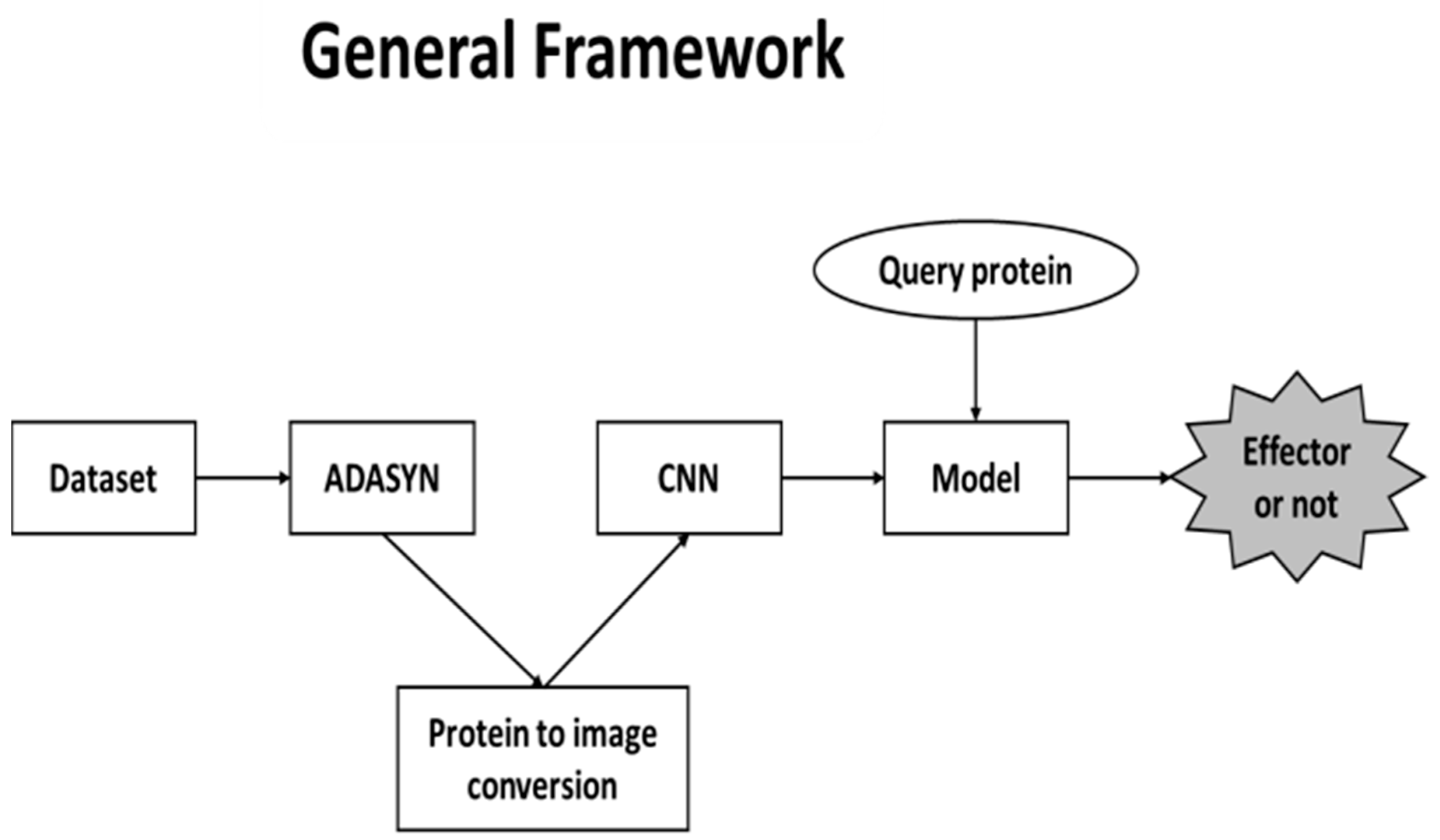
There are three main phases in our proposed framework. First, since the dataset that we used in our study have imbalanced classes, ADASYN was utilized to overcome the issue. As a result, pseudo proteins were generated. After this step, proteins were converted into images to feed the CNN. Conversions were performed by extracting AAC, DPC and PSSM features. All features were represented as matrices and several colors were assigned to each of the amino acids. The final phase was the training part of the CNN. Finally, CNN model was formed to predict whether the query protein is an effector. The general framework structure is shown in Figure 1.
2.2. ADASYN Algorithm
Imbalanced dataset problem arises in cases where some data distributions are dominant in the sample space relative to other data distributions. Machine learning models perform learning based on this predominant data distribution and ignore data distributions of the minority. Thus, models cannot learn minority distributions properly and perform poorly in prediction process. There are many ways to deal with this issue. The first approach is to assign weights to classes to solve this imbalance problem [19,20]. The second approach is creating synthetic samples from minority class so that majority and minority classes have almost 1:1 ratio. An algorithm belonging to the second approach called ADASYN has emerged to solve this imbalanced learning problem.
ADASYN is an enhanced version of the SMOTE (Synthetic Minority Over sampling TEchnique) algorithm to solve imbalanced learning [21]. SMOTE algorithm creates synthetic minority samples to tilt classifier learning bias towards to minority class [22]. Synthetic minority sample creation process in SMOTE uses linear interpolation from existing samples.
ADASYN is based on the idea of creating minority data samples dynamically based on their distribution. More synthetic data are produced for minority class samples that are more difficult to learn. SMOTE synthetic sample creation process produces equal numbers of synthetic samples for each minority data sample, whereas in ADASYN different weights are assigned to different minority samples and therefore the numbers of synthetic samples created are different for every minority sample. ADASYN algorithm reduces the poor performance introduced by the original imbalance data distribution and can also change the decision boundary to focus on difficult-to-learn samples [21]. ADASYN algorithm implementation details are described below [21]:
Input: Training dataset with m samples is represented as where is an instance in n dimension space and is the class label that is associated with . and are number of minority class examples and majority class examples, respectively. Thus, and
Process of ADASYN:
(1) Firstly, degree of class imbalance is calculated
having .
(2) If , then ( represents a threshold for the maximum tolerated degree of class imbalance):
(a) Find the number of synthetic data samples for the minority class that need to be generated:
Here, represents a parameter that specifies the desired level of balance after synthetic data generation. is the result that a fully balanced dataset is created after the generalization phase.
(b) For each example having the condition , Euclidian distance K nearest neighbors is found in n-dimensional space. Ratio is defined as:
where represents the number of samples in the K nearest neighbors of that belong to majority class, thus .
(c) Normalize regarding so that has a density distribution ().
(d) Calculate the number of synthetic data samples that need to be generated for every minority sample
where represents the total number of synthetic data samples that need to generated for the minority class defined in Equation (2).
(e) Generate synthetic data samples () for each minority class data sample () according to the process below:
Loop from 1 to
(i) Randomly choose one minority data sample ( from the K nearest neighbors for data ().
(ii) Generate synthetic data sample:
where represents difference vector in n-dimensional space and is a random number that has range .
2.3. Feature Extraction for Image Representation
The feature extraction process can be considered as a pre-processing stage to represent proteins as images and let CNN take these images as inputs. Amino Acid Composition (AAC), Dipeptide Composition (DPC) and Position-Specific Scoring Matrix (PSSM) composition representation methods were used to extract features from protein sequences [15]. Thus, each protein can be represented as a feature vector. Feature extraction methods are described below.
Let P stand for a protein. In nature, there are 20 types of amino acids, thus AAC of a protein consists of a 20-D vector where each element (aaci) of the feature vector represents the percentage of each amino acid type in the protein. By using this method, a protein can be represented as follows:
P = {aac1, aac2, aac3, …, aac20}
DPC of a protein consists of a 400-D vector where each element (dpci) of the feature vector represents the percentage of each possible amino acid pairs in the protein. By using this method, a protein can be represented as follows:
P = {dpc1, dpc2, dpc3, …, dpc400}
PSSM composition of a protein consists of a 400-D vector where each element (pssmi) of the feature vector represents substitution scores of each amino acid type. In the evolutionary process, each amino acid type is likely to undergo mutation to another amino acid type. Therefore, the substitution scores are important to demonstrate this evolutionary process. Scores indicate that the given amino acid substitution occurs more frequently in the alignment than expected by chance, while negative scores indicate that the substitution occurs less frequently than expected. By using this method, a protein can be represented as follows:
where pssm1 symbolizes substitution score of amino acid 1 (Alanine, A) mutating into amino acid 1 (Alanine, A), pssm2 symbolizes substitution score of amino acid 1 (Alanine, A) mutating into amino acid 2 (Arginine, R), and so on.
P = {pssm1, pssm2, pssm3, …, pssm400}
By using the above feature extraction methods, each protein becomes suitable to be converted into a fixed size image.
2.4. Protein to Image Conversion
Since CNN requires all images to be a fixed size, proteins have to be converted to images. Let I denote a three-dimensional matrix that represents the converted image of a protein. Each dimension corresponds to a different color channel, R, G, and B for red, green and blue, respectively. For AAC, a protein can be defined as follows:
where I = 1, 2, ..., 20. Thus, AAC of a protein is converted into an image that only has values on the diagonal of the matrix. Other pixels that are not present on the diagonal have no color values.
For DPC and PSSM feature vectors, a protein can be defined as follows:
where i = 1, 2, ..., 20 and j = 1, 2 ,..., 20. Subscript 1 (in R1, G1, and B1) denotes the color value of the first amino acid, while subscript 2 (in R2, G2, and B2) denotes the color value of the second amino acid. The final color value is calculated by averaging amino acid pairs. DPC and PSSM have feature vectors of 400 elements. Each section in the feature vector that has 20 elements corresponds to an amino acid type and its values related to other amino acid types; therefore, each section can be placed in a row on the matrix I. All color values assigned to all amino acid types are listed in Supplementary Material Table S1.
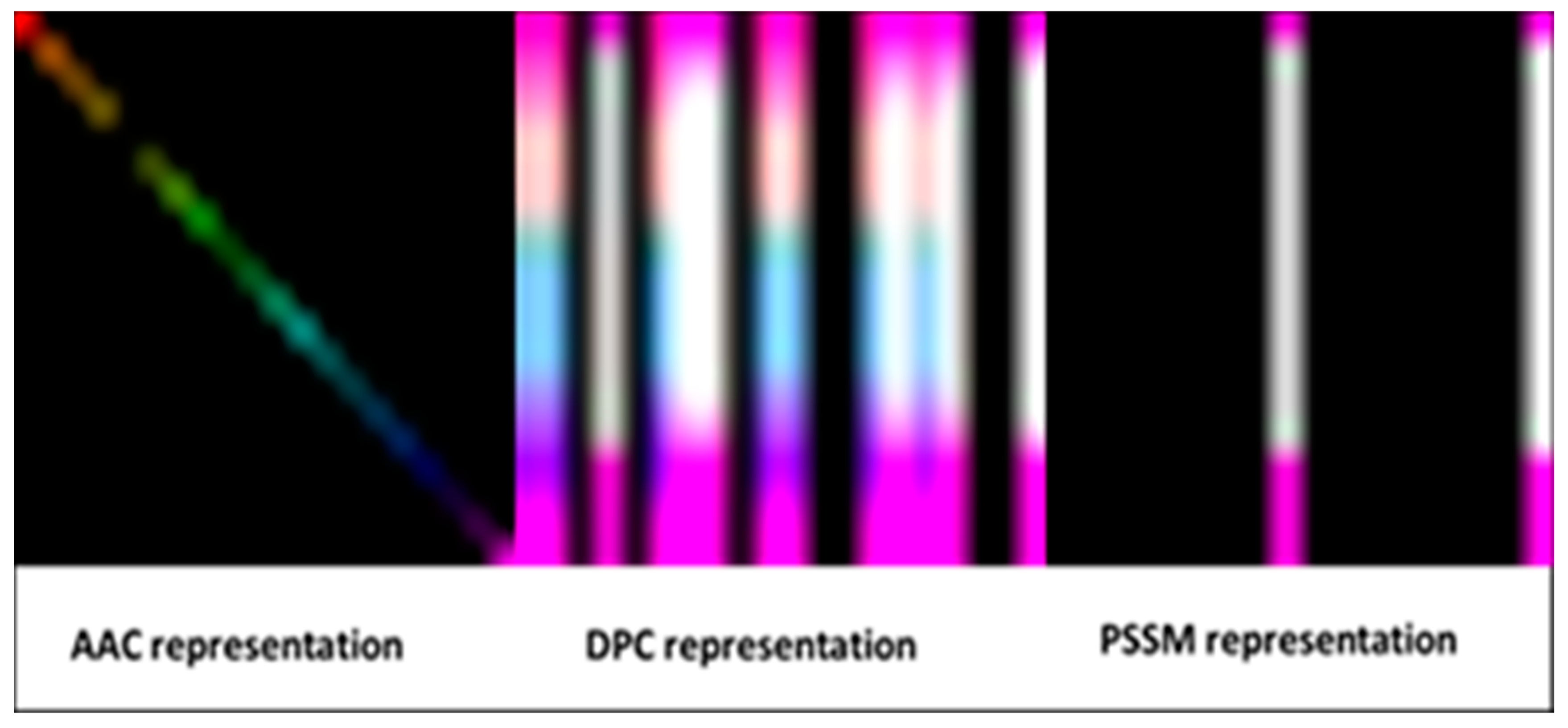
Representations of proteins as images are shown in Figure 2.
2.5. Convolutional Neural Network (CNN)
Unlike other deep learning architectures, artificial neurons in CNNs extract the features of small areas of input images known as receptive fields. Using the knowledge that visual cortex cells are sensitive to small regions of the visual field, the feature extraction process of CNNs was formed [23].
A CNN includes an input, output and multiple hidden layers. Hidden layers generally comprise convolutional layers, pooling layers and fully connected layers. Convolutional and pooling layers are two special types of layers in CNNs [24]. In the convolutional layer, the image is processed by different filters. Filters share the same parameters in every small part of the view. The resulting images of the filters are called feature maps. The pooling layer reduces the variance by capturing average, maximum, or other statistical values of the various regions in the feature maps and captures key features. Fully connected layers work as traditional MLP does, by connecting a neuron in a layer to all neurons in the next layer. In addition, batch normalization and rectified linear unit (ReLU) layers can also be found in CNN. Batch normalization is used to normalize the gradients propagating through the network and it helps accelerate training phase. Batch normalization layer is followed by a ReLU layer that is simply a nonlinear activation function that keeps positive values unchanged and makes negative values zero.
CNN, one of the deep learning architectures, is used especially in image recognition problems and successful results are obtained. If biological structures are represented by images, it becomes possible to apply the CNN architecture to problems of bioinformatics.
3. Results
3.1. Dataset
We used a dataset that Zou et al. [15] constructed from known effectors and non-effectors. The reason for selecting this dataset was based on the ease of performing separate tests on both IVA and IVB effectors. The dataset consists of 30 IVA effectors, 310 IVB effectors and 1132 non-effectors and is referred to as T4_1472. The non-effector proteins represent proteins that do not have an association with pathogenicity and are considered as non-effecting in this manner. It has a ratio of 1:4 of IVB effectors to non-effectors. IVA sequences were collected from nine species and IVB sequences were collected from two species (Table 1). All selected effectors are known to be experimentally validated. This datase is biased. It mainly consists of non-effectors. Thus, to make the dataset more balanced and provide more effective training phase, we applied ADASYN algorithm. Therefore, the biased dataset problem and class imbalance problem were solved by creating more minority class proteins.
3.2. Experimental Setup
ADASYN was used to increase the ratio to about 1:1 of effectors to non-effectors. For each of the feature extraction methods, different numbers of pseudo proteins were generated. Table 2 shows the distribution of pseudo proteins according to the feature extraction methods and effector types.
After extracting features for AAC, DPC and PSSM, different color values were assigned for all amino acids to represent the images for proteins.
In addition to representations with AAC, DPC and PSSM, we prepared six more representation scenarios to determine the colors of amino acid types. There were two ideas behind these scenarios. First, to determine how different coloring schemes affect prediction performance, we assigned different colors to different group of proteins. Second, by assigning shades of colors to proteins in the same group, we aimed to find how color shade parameter affects predicting proteins and as well as CNN’s discriminative behavior.
For scenario 1 (Sc1), all hydrophobic amino acids were represented as red, hydrophilic ones as green, and amphipathic as blue.
Scenario 2 (Sc2) is a modified version of Sc1. Instead of using single colors, shades of red were given to hydrophobics, shades of green to hydrophilics and shades of blue to amphipathics.
Scenario 3 (Sc3) was based on Sc1 but amphipathics were discarded. No color value was given to them. They were represented as black.
Scenario 4 (Sc4) was based on Sc2 but amphipathics were also discarded. They were represented as black.
For Scenario 5 (Sc5), we considered subclasses of hydrophobic amino acids. Aliphatic, simple, cyclic and aromatic amino acids were represented with different colors. Other amino acids without considering their classes were also given different colors.
Scenario 6 (Sc6) is a modified version of Sc5. The only difference is that aliphatic amino acids were assigned shades of red.
Color values for all representation scenarios are presented in Supplementary Material Table S1.
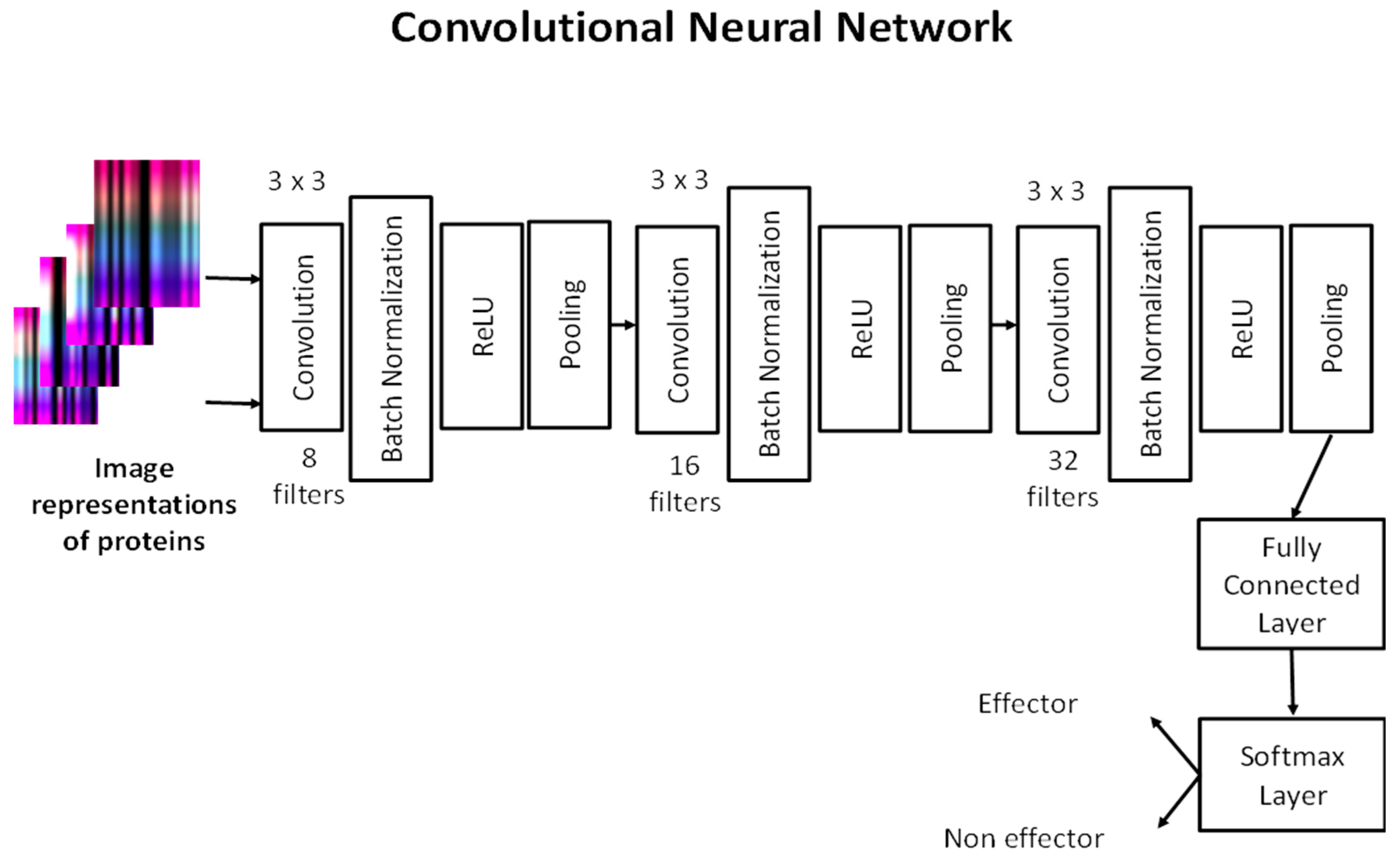
We built a CNN architecture to predict T4SS effector proteins. Our network consists of three convolutional layers. Each convolutional layer has 8, 16 and 32 filters, respectively, with size 3 × 3. After each convolutional layer, batch normalization, ReLU and max-pooling layers exist, except in the last convolutional layer. The fully connected layer combines the learned features to classify the images that represent proteins. The softmax layer calculates classification probabilities to predict whether an image belongs to effector or non-effector protein classes. Our CNN architecture is shown in Figure 3.
3.3. Evaluation
Leave One Out (LOO) cross-validation tests were used to assess all protein representation methods. According to the LOO strategy, a sample is accepted as query instances (test set) while other samples in the dataset as training set. A model is constructed from the training samples and query instance is compared to the model. This process continues until all of the samples have been queried in this manner.
Six different metrics were used to evaluate the performance of the classification: sensitivity, specificity, accuracy, Matthew’s correlation coefficient, Youden’s J Statistic, and F1 Score. TP, TN, FP and FN refer to the number of true positives, true negatives, false positives and false negatives, respectively.
Sensitivity (Sn) is the ratio between correctly classified effectors and all effectors:
Specificity (Sp) is the ratio between correctly classified non-effectors and all non-effectors:
Accuracy (Acc) is the ratio between correctly classified non-effectors and effectors and all samples:
The Matthew’s correlation coefficient (MCC) measures the quality of classification:
Youden’s J Statistic (J Stat.) is measured as follows:
F1 score is the harmonic average of the precision and recall:
F1 score is also calculated as:
3.4. Empirical Results
The evaluation results of LOO cross-validation experiments when protein representation models are applied for the effector (IVA and IVB) prediction are given in Supplementary Materials Tables S2–S5.
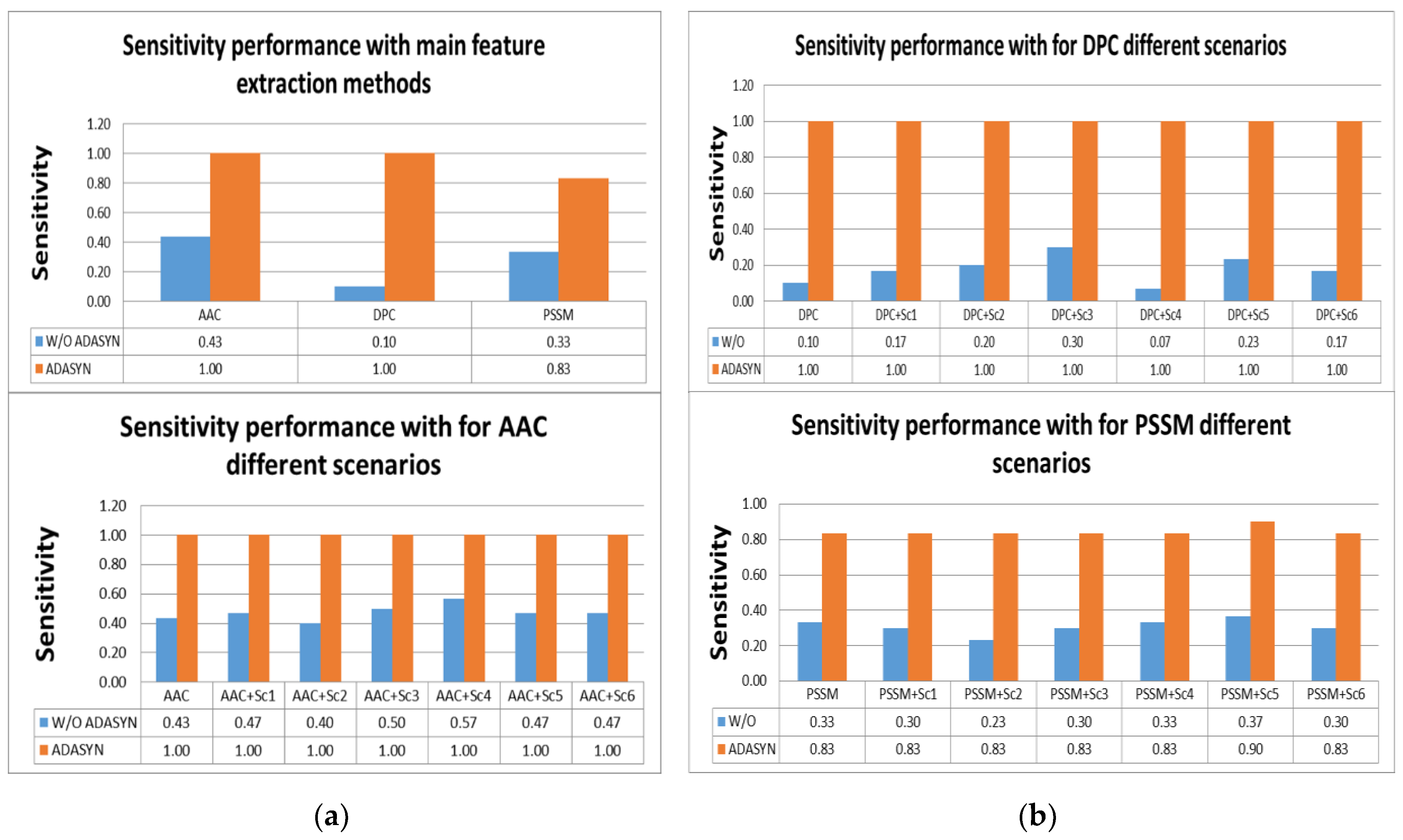
According to Tables S2 and S3, the highest scores for sensitivity measure were obtained by using AAC and DPC with ADASYN apposition. All effectors were predicted correctly with them. In addition, using all scenarios for AAC and DPC predicted all IVA effectors. It was shown that utilizing ADASYN algorithm for all protein representation methods and scenarios was superior to all methods without ADASYN. For other metrics, all representations and scenarios gave better performance than PSSM and variations. Comparison of representation methods for IVA in terms of sensitivity metric is shown in Figure 4a,b.
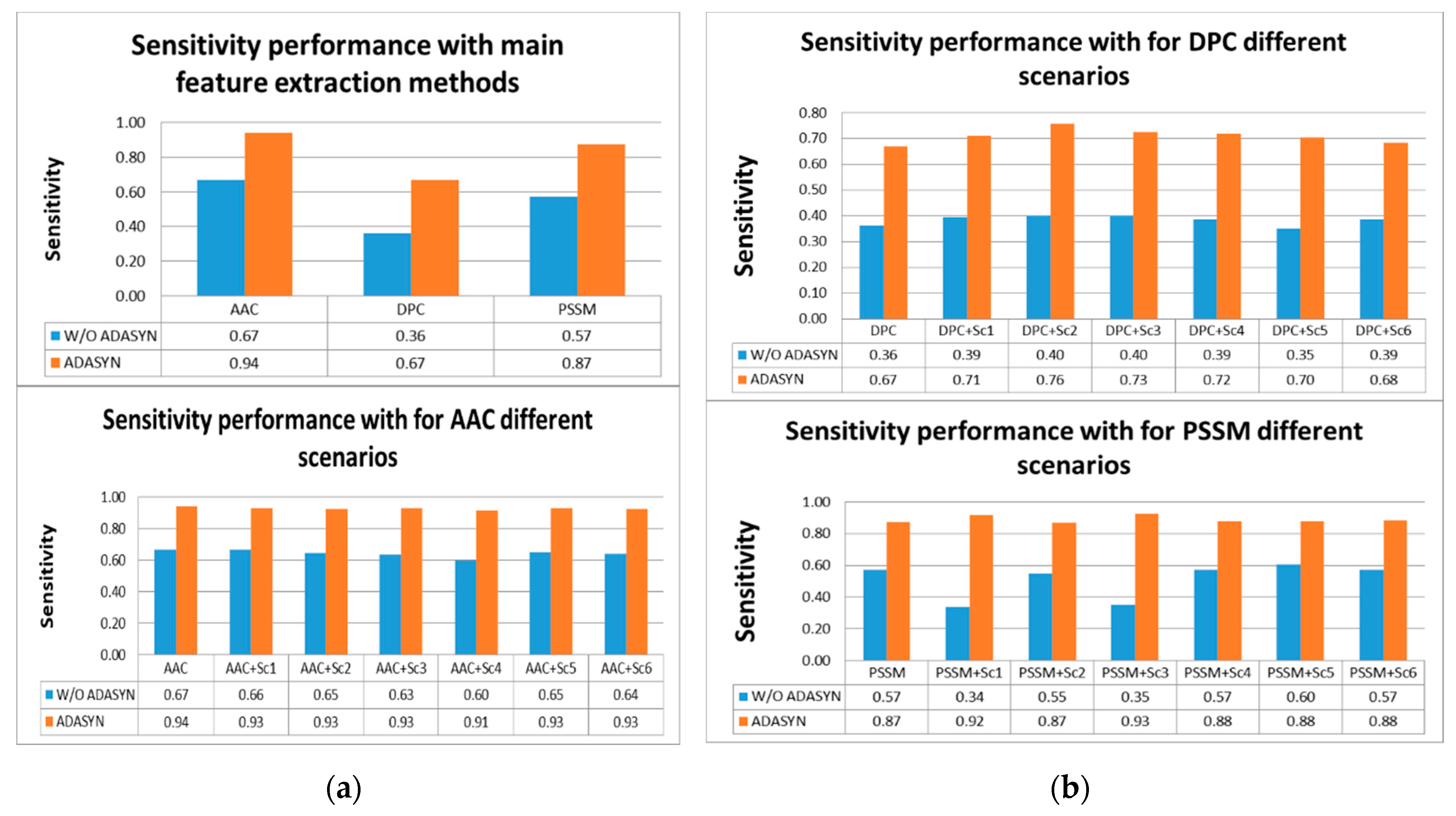
According to Tables S4 and S5, the highest score for sensitivity measure was obtained using AAC with ADASYN apposition. The second highest score was achieved by PSSM with ADASYN without considering representation scenarios. DPC with ADASYN had the lowest score. It was shown that representation scenarios for AAC and PSSM with ADASYN gave better results than DPC and its variations. It was found that utilizing ADASYN algorithm was superior to others without ADASYN. For other metrics, AAC with ADASYN had the best performance values. In addition, representation scenarios for AAC and PSSM with ADASYN gave close results to AAC with ADASYN. Comparison of representation methods for IVB in terms of sensitivity metric is shown in Figure 5a,b.
When we compared our approach with our original research [15], it was revealed that we improved the classification performance of the original one in terms of sensitivity. This result can be interpreted as deep learning architectures can exploit the image representation of proteins. Extracting image features can be more effective than raw AAC protein representations in terms of sensitivity. Therefore, it can be said that this study provides a baseline for applying CNN architectures to T4SS protein prediction problem. The comparison of the best performances for two studies is given in Table 3. Sensitivity performance was increased by about 3%.
4. Conclusions and Discussion
The contribution of this study is fourfold. First, the proposed approach offers a deep learning-based framework to predict T4SS effector proteins. Thus far, all studies on T4SS use traditional machine learning methods. We demonstrated the usability of CNN, one of the deep learning architectures. Second, we showed that protein to image conversion, using AAC, DPC and PSSM feature extraction methods, is applicable to classification problems in bioinformatics. Proteins can be represented as images and used as inputs for deep learning. Third, generating pseudo proteins, in a situation where unbalanced classes exist in a dataset, is advantageous for classification while working with CNN. ADASYN algorithm solved this imbalanced dataset issue in protein prediction problem. The algorithm created new samples for effector proteins, which are a minority class in this situation, and balanced the dataset distribution; therefore, a more corrective and accurate classification procedure was implemented. In addition, by increasing the number of samples with this algorithm, the deep learning architecture we used had more variant data to train on, and therefore a significant increase in performance was observed using ADASYN. Fourth, grouping amino acid types according to their hydrophobicity yielded close results to the best one, which was obtained using AAC. AAC yielded better results because AAC of a protein consists of features where each element of the feature vector represents the percentage of each amino acid type in the protein. This information is better than features that include protein pairs because it adds information to the feature vector of only one protein and not a pair. These results show that the percentage of one protein in an amino acid representation is better than other representations. Grouping amino acids according to their hydrophobicity yielded better results because using different shades for different subgroups made the CNN network more discriminative. Shading could increase the variance of protein samples, therefore CNN better learned the data and the training process was more effective.
We hope that this study could be an introduction to utilize CNN on T4SS effector recognition as well as other secretion systems for researchers. Utilization of deep learning networks has advantages: instead of extracting handmade features in traditional machine learning, deep learning architecture extracts features automatically and classifies them. In addition, by representing proteins with images and feeding them into CNN is more meaningful than traditional feature extraction methods in terms of classification performance. However, deep learning networks also have a disadvantage: they require many data to be successful and much parameter tuning is required for success.
This framework could be improved by combining features to represent a protein with more than three-dimensional matrixes. Another improvement might be to include other deep learning architectures such as Long-Short Term Memory (LSTM) networks and Deep Belief Networks (DBN). Applying majority voting on results of the different architectures may achieve performance increase. Different traditional machine learning approaches and feature extraction methods [25,26] can be used to increase the classification performance as well. In addition, trying different CNN architectures and applying parameter tunings to explore the effects of layer size and parameter selection can be considered to improve performance.
Supplementary Materials
The following are available online at https://0-www-mdpi-com.brum.beds.ac.uk/2306-5729/4/1/45/s1.
Author Contributions
The following statements should be used “methodology, K.A., T.A, Ç.B.E.; validation, H.O.; data curation, K.A.; writing—original draft preparation, K.A, T.A.; writing—review and editing, K.A, T.A., Ç.B.E.; supervision, H.O.
Funding
This research received no external funding.
Conflicts of Interest
The authors declare no conflict of interest.
References
- Green, E.R.; Mecsas, J. Bacterial secretion systems: An overview. Microbiol. Spectr. 2016, 4. [Google Scholar] [CrossRef]
- Fronzes, R.; Christie, P.J.; Waksman, G. The structural biology of type IV secretion systems. Nat. Rev. Microbiol. 2009, 7. [Google Scholar] [CrossRef] [PubMed]
- Juhas, M.; Crook, D.W.; Hood, D.W. Type IV secretion systems: Tools of bacterial horizontal gene transfer and virulence. Cell. Microbiol. 2008, 10, 2377–2386. [Google Scholar] [CrossRef]
- Hatakeyama, M.; Higashi, H. Helicobacter pylori CagA: A new paradigm for bacterial carcinogenesis. Cancer Sci. 2005, 96, 835–843. [Google Scholar] [CrossRef] [PubMed]
- Burns, D.L. Type IV transporters of pathogenic bacteria. Curr. Opin. Microbiol. 2003, 6, 1–6. [Google Scholar] [CrossRef]
- Cascales, E.; Christie, P.J. The versatile bacterial type IV secretion systems. Nat. Rev. Microbiol. 2003, 1, 137–149. [Google Scholar] [CrossRef] [Green Version]
- Zhu, J.; Oger, P.M.; Schrammeijer, B.; Hooykaas, P.J.; Farrand, S.K.; Winans, S.C. The bases of crown gall tumorigenesis. J. Bacteriol. 2002, 182, 3885–3895. [Google Scholar] [CrossRef]
- Seubert, A.; Hiestand, R.; de la Cruz, F.; Dehio, C. A bacterial conjugation machinery recruited for pathogenesis. Mol. Microbiol. 2003, 49, 1253–1266. [Google Scholar] [CrossRef] [PubMed] [Green Version]
- Schulein, R.; Dehio, C. The VirB/VirD4 type IV secretion system of Bartonella is essential for establishing intraerythrocytic infection. Mol. Microbiol. 2002, 46, 1053–1067. [Google Scholar] [CrossRef] [Green Version]
- Boschiroli, M.L.; Ouahrani-Bettache, S.; Foulongne, V.; Michaux-Charachon, S.; Bourg, G.; Allardet-Servent, A.; Cazevieille, C.; Lavigne, J.P.; Liautard, J.P.; Ramuz, M.; et al. Type IV secretion and Brucella virulence. Vet. Microbiol. 2002, 90, 341–348. [Google Scholar] [CrossRef]
- Lawley, T.D.; Klimke, W.A.; Gubbins, M.J.; Frost, L.S. F factor conjugation is a true type IV secretion system. FEMS Microbiol. Lett. 2003, 224, 1–15. [Google Scholar] [CrossRef] [Green Version]
- Christie, P.J.; Atmakuri, K.; Krishnamoorthy, V.; Jakubowski, S.; Cascales, E. Biogenesis, architecture, and function of bacterial type IV secretion systems. Annu. Rev. Microbiol. 2005, 59, 451–485. [Google Scholar] [CrossRef] [PubMed]
- Juhas, M.; Crook, D.W.; Dimopoulou, I.D.; Lunter, G.; Harding, R.M.; Ferguson, D.J.; Hood, D.W. Novel type IV secretion system involved in propagation of genomic islands. J. Bacteriol. 2007, 189, 761–771. [Google Scholar] [CrossRef] [PubMed]
- Burstein, D.; Zusman, T.; Degtyar, E.; Viner, R.; Segal, G.; Pupko, T. Genome-scale identification of Legionella pneumophila effectors using a machine learning approach. PLoS Pathog. 2009, 5, e6974. [Google Scholar] [CrossRef] [PubMed]
- Zou, L.; Nan, C.; Hu, F. Accurate prediction of bacterial type IV secreted effectors using amino acid composition and PSSM profiles. Bioinformatics 2013, 29, 3135–3142. [Google Scholar] [CrossRef] [Green Version]
- Wang, Y.; Wei, X.; Bao, H.; Liu, S.L. Prediction of bacterial type IV secreted effectors by C-terminal features. BMC Genomics 2014, 15, 1–14. [Google Scholar] [CrossRef]
- Zou, L.; Chen, K. Computational prediction of bacterial type IV-B effectors using C-terminal signals and machine learning algorithms. In Proceedings of the 2016 IEEE Conference on Computational Intelligence in Bioinformatics and Computational Biology (CIBCB), Chiang Mai, Thailand, 5–7 October 2016; pp. 1–5. [Google Scholar]
- Wang, J.; Yang, B.; An, Y.; Marquez-Lago, T.; Leier, A.; Wilksch, J.; Hong, Q.; Zhang, Y.; Hayashida, M.; Akutsu, T.; et al. Systematic analysis and prediction of type IV secreted effector proteins by machine learning approaches. Brief. Bioinform. 2017, 1–21. [Google Scholar] [CrossRef] [PubMed]
- Duan, J.; Schlemper, J.; Bai, W.; Dawes, T.J.W.; Bello, G.; Doumou, G.; De Marvao, A.; O’Regan, D.P.; Rueckert, D. Deep Nested Level Sets: Fully Automated Segmentation of Cardiac MR Images in Patients with Pulmonary Hypertension. In Medical Image Computing and Computer Assisted Intervention—MICCAI 2018, Proceedings of the International Conference on Medical Image Computing and Computer-Assisted Intervention, Granada, Spain, 16–20 September 2018; Springer: Cham, Switzerland, 2018; Volume 11073, pp. 595–603. [Google Scholar]
- Duan, J.; Bello, G.; Schlemper, J.; Wenjia, B.; Dawes, T.J.W.; Biffi, C.; De Marvao, A.; Doumou, G.; O’Regan, D.P.; Rueckert, D. Automatic 3D bi-ventricular segmentation of cardiac images by a shape-refined multi-task deep learning approach. IEEE Trans. Med. Imaging 2019. [Google Scholar] [CrossRef] [PubMed]
- He, H.; Bai, Y.; Garcia, E.A.; Li, S. ADASYN: Adaptive synthetic sampling approach for imbalanced learning. In Proceedings of the 2008 IEEE International Joint Conference on Neural Networks (IEEE World Congress on Computational Intelligence), Hong Kong, China, 1–8 June 2008; pp. 1322–1328. [Google Scholar]
- Chawla, N.V.; Hall, L.O.; Bowyer, K.W.; Kegelmeyer, W.P. SMOTE: Synthetic Minority Oversampling Technique. J. Artif. Intell. Res. 2002, 16, 321–357. [Google Scholar] [CrossRef]
- Ciresan, D.; Meier, U.; Schmidhuber, J. Multi-column deep neural networks for image classification. In Proceedings of the IEEE Conference on Computer Vision and Pattern Recognition (CVPR), Washington, DC, USA, 16–21 June 2012; pp. 3642–3649. [Google Scholar]
- Cao, C.; Liu, F.; Tan, H.; Song, D.; Shu, W.; Li, W.; Zhou, Y.; Bo, X.; Xie, Z. Deep Learning and its Applications in Biomedicine—Genomics. Prot. Bioinform. 2018, 16, 17–32. [Google Scholar]
- Ding, Y.; Pardon, M.C.; Agostini, A.; Faas, H.; Duan, J.; Ward, W.O.C.; Easton, F.; Auer, D.; Bai, L. Novel Methods for Microglia Segmentation, Feature Extraction, and Classification. IEEE/ACM Trans. Comput. Biol. Bioinform. 2017, 14, 1366–1377. [Google Scholar] [CrossRef] [PubMed] [Green Version]
- Yang, D.; Subramanian, G.; Duan, J.; Gao, S.; Bai, L.; Chandramohanadas, R.; Ai, Y. A portable image-based cytometer for rapid malaria detection and quantification. PLoS ONE 2017, 12, e0179161. [Google Scholar] [CrossRef] [PubMed]
Figure 1.
General framework structure.

Figure 2.
Representations of proteins according to different feature extraction methods.

Figure 3.
Convolutional Neural Network CNN architecture.

Figure 4.
(a) Sensitivity performance for IVA effectors. (b) Sensitivity performance for IVA effectors.
Figure 4.
(a) Sensitivity performance for IVA effectors. (b) Sensitivity performance for IVA effectors.

Figure 5.
(a) Sensitivity performance for IVB effectors. (b) Sensitivity performance for IVB effectors.
Figure 5.
(a) Sensitivity performance for IVB effectors. (b) Sensitivity performance for IVB effectors.


Table 1.
Numbers of effector proteins according to species.
| Numbers of Effector Proteins | ||
|---|---|---|
| Species | IVA | IVB |
| A. marginale | 4 | - |
| Anaplasma phagocytophilum | 2 | - |
| Bartonella sp. | 3 | - |
| H. pylori | 1 | - |
| Agrobacterium tumefacien | 3 | - |
| Agrobacterium rhizogenes | 4 | - |
| Brucella sp. | 8 | - |
| B. pertussis | 4 | - |
| E. chaffeensis | 1 | - |
| L. pneumophila | - | 258 |
| C. burnetii | - | 52 |
| TOTAL | 30 | 310 |
Table 2.
Number of generated pseudo proteins using ADASYN algorithm.
| Effector Types | ||||||||
|---|---|---|---|---|---|---|---|---|
| IVA | IVB | |||||||
| Feature Extraction Methods | Effectors (Minority Class) | Generated Pseudo Proteins | Non-Effectors (Majority Class) | Effector: Non-Effector Ratio | Effectors (Minority Class) | Generated Pseudo Proteins | Non-Effectors (Majority Class) | Effector: Non-Effector Ratio |
| AAC | 30 | 1098 | 1132 | 0.996 | 310 | 853 | 1132 | 1.027 |
| DPC | 30 | 1105 | 1132 | 1.003 | 310 | 811 | 1132 | 0.990 |
| PSSM | 30 | 1100 | 1132 | 0.998 | 310 | 821 | 1132 | 0.999 |
Table 3.
Performance comparison for IVB with previous work.
| Sn | Sp | Acc | MCC | J stat. | F1 | |
|---|---|---|---|---|---|---|
| Zou et al. [15] * | 0.916 | 0.996 | 0.979 | 0.936 | NR | NR |
| Our study | 0.942 | 0.903 | 0.911 | 0.774 | 0.840 | 0.820 |
* Ten-fold CV tests were performed on the dataset. We used LOO tests. Their best performance was achieved by 2 in 3 voting scheme with 3 SVM classifiers. We used only a CNN for classification. (NR: Not Reported).
© 2019 by the authors. Licensee MDPI, Basel, Switzerland. This article is an open access article distributed under the terms and conditions of the Creative Commons Attribution (CC BY) license (http://creativecommons.org/licenses/by/4.0/).
Share and Cite
MDPI and ACS Style
Açıcı, K.; Aşuroğlu, T.; Erdaş, Ç.B.; Oğul, H. T4SS Effector Protein Prediction with Deep Learning. Data 2019, 4, 45. https://0-doi-org.brum.beds.ac.uk/10.3390/data4010045
AMA Style
Açıcı K, Aşuroğlu T, Erdaş ÇB, Oğul H. T4SS Effector Protein Prediction with Deep Learning. Data. 2019; 4(1):45. https://0-doi-org.brum.beds.ac.uk/10.3390/data4010045
Chicago/Turabian StyleAçıcı, Koray, Tunç Aşuroğlu, Çağatay Berke Erdaş, and Hasan Oğul. 2019. "T4SS Effector Protein Prediction with Deep Learning" Data 4, no. 1: 45. https://0-doi-org.brum.beds.ac.uk/10.3390/data4010045