Diagnosis of Intermittently Faulty Units at System Level


1
Department Informatics, Faculty of Science, University of J.E.Purkyne, Pasteurova 3544/1, 40096 Usti nad Labem, Czech Republic
2
Department Informatics and Computer Science, Faculty of Cybernetics and System Engineering, Kherson National Technical University, Bereslavskoe highway 24, 73008 Kherson, Ukraine
*
Author to whom correspondence should be addressed.
Data 2019, 4(1), 44; https://0-doi-org.brum.beds.ac.uk/10.3390/data4010044
Submission received: 3 March 2019
/
Revised: 16 March 2019
/
Accepted: 17 March 2019
/
Published: 22 March 2019
(This article belongs to the Special Issue Data Stream Mining and Processing)
Abstract
:Mostly, diagnosis at a system level intends to identify only permanently faulty units. In the paper, we consider the case when both permanently and intermittently faulty units can occur in the system. Identification of intermittently faulty units has some specifics which we have considered in this paper. We also suggest the method which allows for distinguishing among different types of intermittent faults. A diagnosis procedure was suggested for each type of intermittent fault.
1. Introduction
Recent advances in semiconductor technology allow the designing of powerful single-chip microprocessors. Since the cost of microprocessor systems has considerably reduced, we are able to build more and more sophisticated microprocessor systems with up to thousands of microprocessors.
Developing many-core processors with novel architectures enables the increasing of the processor performance [1]. To achieve such an effect, a novel architecture should provide interactions among processor cores and the execution of many tasks simultaneously.
Increasing possibilities of emerged many-core processors result in their broad deployment in different areas. It, in its turn, imposes the high requirements of dependability of many-core processors [2].
To provide processor fault-tolerance, different methods can be applied. All of them have some mutual features. First of all, error detection should be performed. Usually, error detection results in a signal or message indicating the erroneous state of the processor. After that, a recovery of the processor state is performed (error handling). Error handling can be carried out either by way of backward error recovery or forward error recovery or masking. Masking requires different types of redundancy. Hardware redundancy implies redundant processor cores. Information redundancy exploits different coding techniques. Time redundancy consists of repeating some computation on the same hardware.
After error handling, fault handling can be performed. It is worth noting that fault handling can be omitted. It depends on the chosen way of error handling. The main steps of fault handling are as follows: fault diagnosis; fault isolation; processor reconfiguration; and reinitialization.
For providing fault handling, built-in testing capabilities (so-called built-in-self-test schemes) are often used. Built-in testing allows the efficient performance of fault handling [3]. Unfortunately, the wide applicability of built-in testing is undermined by the need to have some part of the processor (called the hard-core) operational even in the presence of a fault.
Self-diagnosis, which uses the ability of processor cores to test each other, is now actively studied as a promising technique for providing processor core checking and diagnosis [4,5,6,7].
The basis for the diagnosis of intermittent faults at a system level was developed by Mallela and Masson [8]. They determined the condition (in this paper, denoted as RΣ ∈ R0) which should be used in the diagnosis algorithms, taking into account intermittent faults.
It worth noting that the authors did not consider the problem of implementation of the suggested method. In this paper, we present an efficient algorithm allowing us to perform verification of above-mentioned condition. Moreover, we have also determined what should be done when the condition is not satisfied.
We assume that the suggested method in the paper begins to diagnose intermittent faults that can be used not only for many-core processors but also for a wide range of complex systems, which employ self-diagnosis.
It is worth noting that diagnosis of system units at a system level considers a fault in the system as a failure of a system unit. We do not consider the details of what was wrong with the failed unit as it was done, for example, in the fault diagnosis described in [9,10,11]. In view of this, we do not classify the faults as it was done, for example, in [12,13]. In essence, we consider each system unit as either failed or correct (which is denoted as “1” or “0”). Failure of the system occurs when the total number of failed units exceed the maximum value determined in advance.
The paper is organized as follows. Section 2 presents the model and classification of intermittent faults in the context of self-diagnosis. Section 3 describes the problems of developing diagnosis algorithms when intermittent faults can take place. In Section 4, it is shown how intermittently faulty units can be diagnosed on the basis of the obtained syndrome. Section 5 presents our approach to formation of all potential syndromes and to verifying the main condition. Section 6 shows what could be done if the main condition is not met. Conclusions are given in the final section.
2. Related Work
Diagnosis of intermittent faults in electric mechanical and electronic devises is well studied and presented in a number of papers (e.g., [14,15]). Normally, such diagnosis employs external facilities for providing testing and analysis. As distinct from these researches we consider the systems which units are capable of performing both testing and diagnosis algorithms.
Recently, a comparisons based approach is widely used to detect both permanent and intermittent faults in the networks [16]. Application of comparison-based model in sensor networks allows a sensor node to identify its own status based on the information received from the neighbors [17,18,19]. As another possibility, the state of a node can be diagnosed by the other system nodes [20,21]. It is worth noting that these researches mostly deal with homogeneous systems and/or use very much simplified local diagnosis in relation to intermittent faults.
The advances achieved in modern electronics made it possible to better handle the obtained diagnosis syndromes. Particularly, now it is possible to present the algorithms at high level of abstraction with generation of code that exploits the inherent parallelism of current CPU (including the vectorization) [22]. Namely, this was done by us in the paper.
3. Classification of Intermittent Faults in the Context of Self-Diagnosis
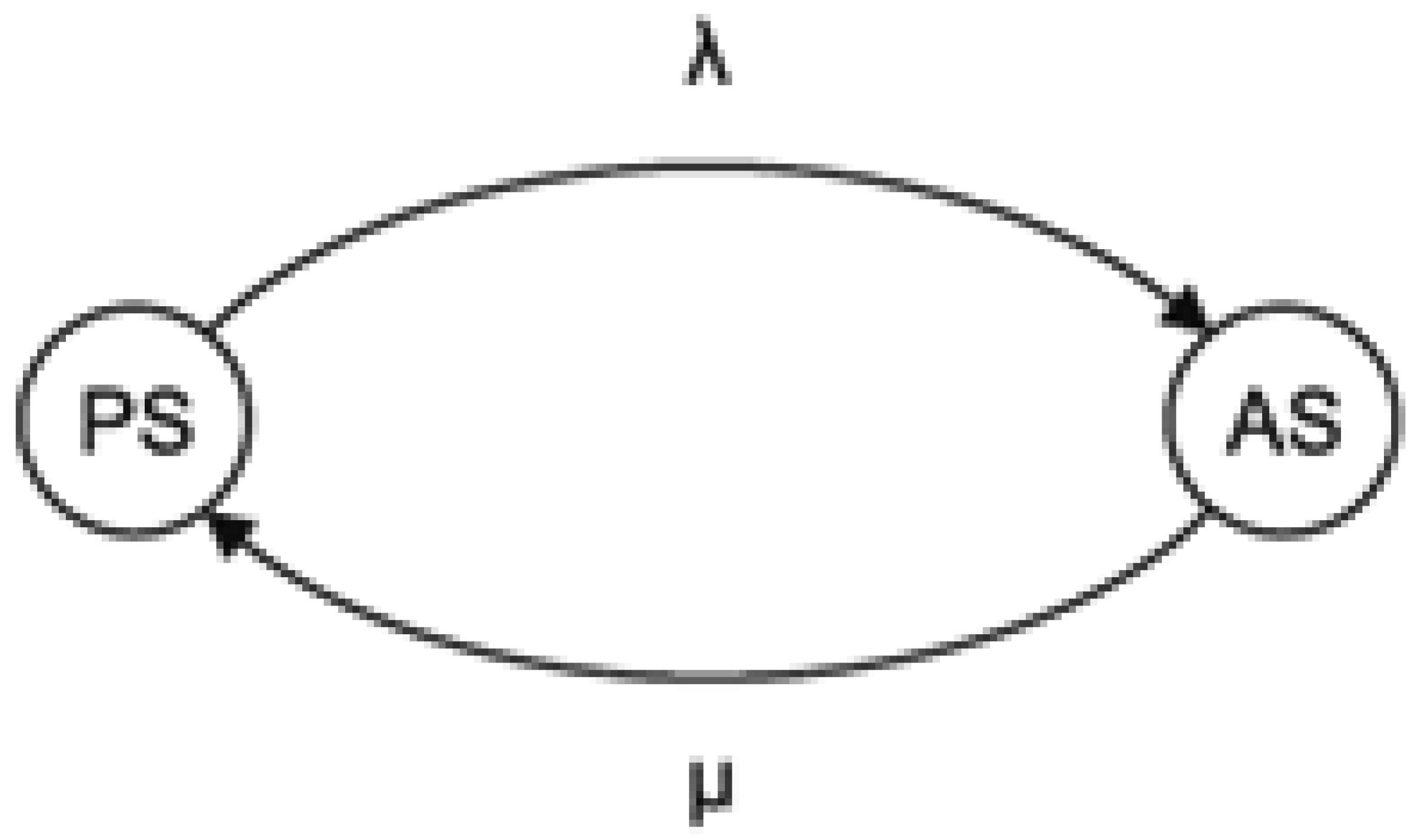
Intermittent fault of a system unit can be defined as a fault, which randomly transfers from a latent state to an active state and vice versa. There exist several models, which describe the behavior of an intermittent fault [8,23]. We use the model proposed in [8]. In this model, the behavior of intermittent fault is expressed by continuous Markov chain, where the time during which an intermittent fault stays in active, respectively passive state, is random value with exponential distribution (see Figure 1).
In Figure 1, and denote the rates of transition from passive to active state and vice versa.
When an intermittent fault is in active state it can course an error in a system unit and affect the tests related to the erroneous unit.
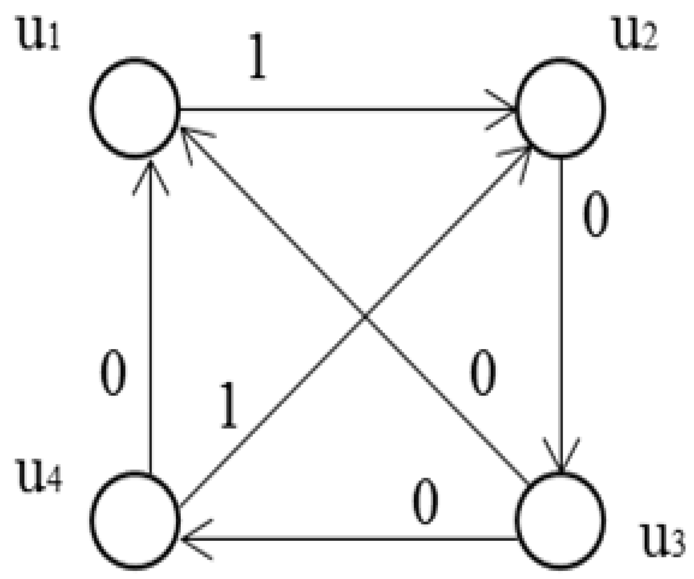
System level self-diagnosis deals with the mutual testing. In this case, one of the system units performs tests on the other units. Convenient form for representing a mutual testing is graph model (testing graph). Example of testing graph is shown in Figure 2.
In the given case, diagnosable system consists of four units U = {u1, u2, u3, u4}. Each unit ui, ui ∈ U, is assigned a particular subset of units in U to test.
Generally, a unit can test itself. Although, we assume that a unit doesn’t do this. In the corresponding testing graph, it means the absence of loops (i.e., testing graph doesn’t contain the edges that connect a vertex to itself).
A test, which invokes two units, is represented in the testing graph by the edge between two vertices which correspond to testing and tested units. In Figure 2, there are six edges. These edges correspond to tests τ12, τ23, τ34, τ41, τ31 and τ42. Subscripts point to the units that are involved in the test. The complete collection of tests is called a testing assignment. Test result is represented by binary variable rij which can take values 0 or 1. Variable rij is equal to 0 if unit ui evaluates unit uj as fault-free. Otherwise, rij = 1.
In Figure 2, test results are shown next to the corresponding edges. The set of test results is called a syndrome. Identification of faulty units using a syndrome is called diagnosis.
Generally, for providing diagnosis at system level some assumptions are made, such as:
- tests can be performed only in the periods of time when system units do not perform their proper system functions (i.e., when they are in idle state). That is, a system unit is not tested continuously, and, therefore, there exists a probability of not detecting the failed unit;
- even if a unit is failed, a test not always detects this event. It depends on test coverage;
- result of a test is expressed as 0 or 1 depending on the evaluation of the testing unit about the state of the tested unit;
- tests in a system can be performed either according to a predefined testing assignment or randomly.
In this paper, we consider that test coverage is equal to 100%. We also assume that tests among system units are performed according to predefined testing assignment. It means that the total time of testing is known beforehand. Consequently, the periods of time when each unit is involved in tests are also known in advance.
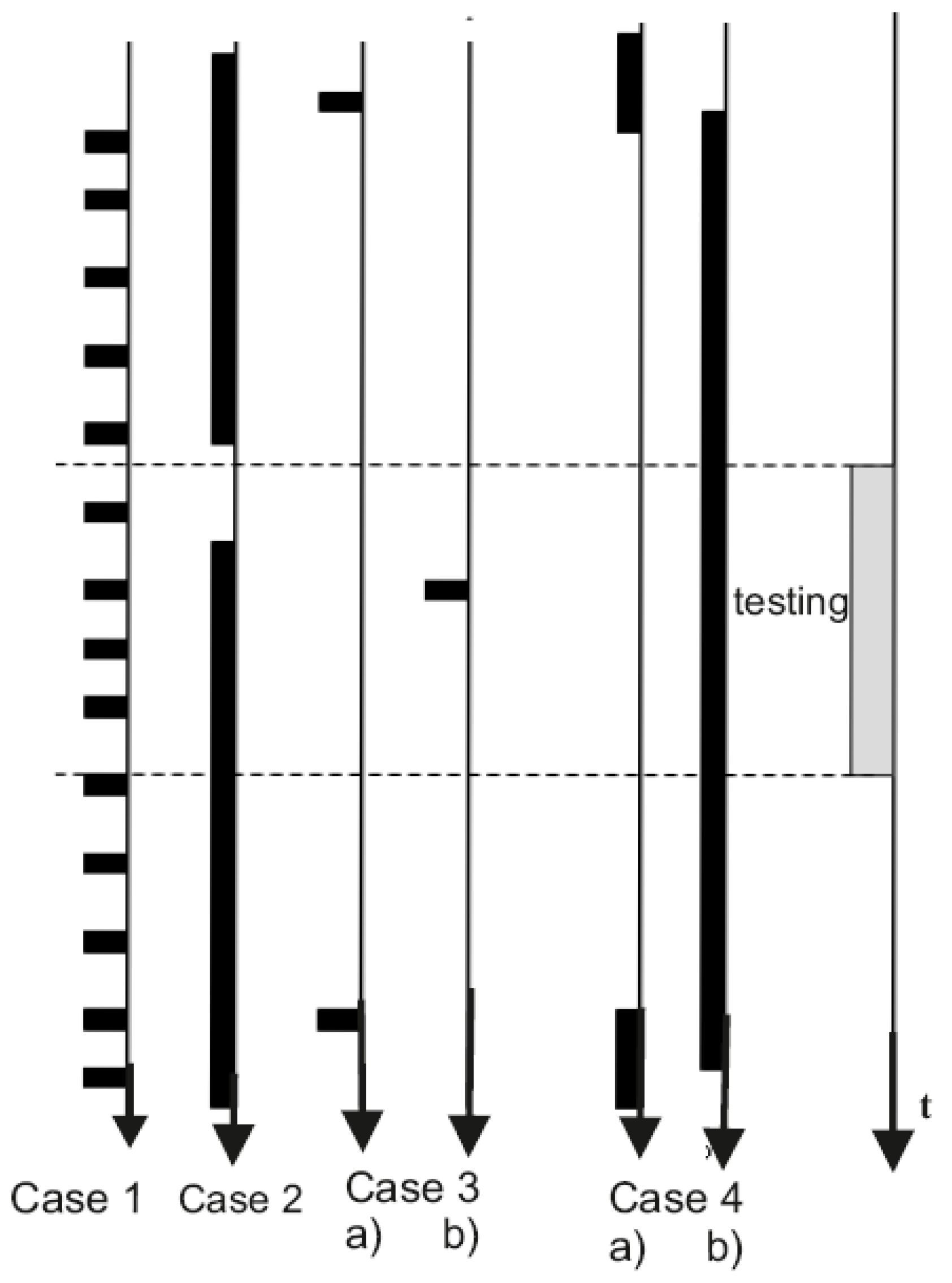
In the given case, it is possible to consider parameters of intermittent fault model (i.e., λ and μ) in relation to the total time of testing, ttesting. Table 1 presents possible evaluations of values 1/ λ and 1/μ as compared to the value of ttesting. This comparison bears some resemblance to the techniques based on fuzzy logic. We evaluate the values of 1/ λ and 1/μ as “large” and “small” depending on the ratios of values 1/λ (1/μ) and ttesting.
As a result of this consideration, it is possible to divide the considered intermittent faults into several classes.
Intermittent faults related to class 1 and class 2 can be detected with high probability during testing procedure. Detection of intermittent faults in case 3 is very improbable (problematic). Probability of detecting such faults is low. As concerns case 4, there exist two options— a) and b) (see Figure 3). In the given case, probability of intermittent fault detection can be estimated as 0.5 when 1/λ ≈ 1/μ.
Generally, system level self-diagnosis is aimed at detecting permanently faulty system units. Nevertheless, there exist the possibility to detect also intermittently faulty units when intermittent faults are related to classes 1,2 and 4 [24].
4. Problems with Developing Diagnosis Algorithms When Intermittent Faults are Allowed
Diagnosis is performed on the basis of obtained syndrome. A syndrome is a set of test results. The result of test τij is denoted as rij and can take the values 0 or 1 depending on the fact of how unit ui evaluates the state of unit uj.
In the paper, we accept the evaluation proposed by Preparata [25].
We also assume that if an intermittent fault is in an active state, then the unit with this fault behaves as permanently faulty unit.
To explain the problems with diagnosis made on the basis of the obtained syndrome, let us consider a simple example with code in Julia programming language. We have implemented our solution in this programming language for illustration of how bitwise operations can effectively represent the operations on the syndrome.
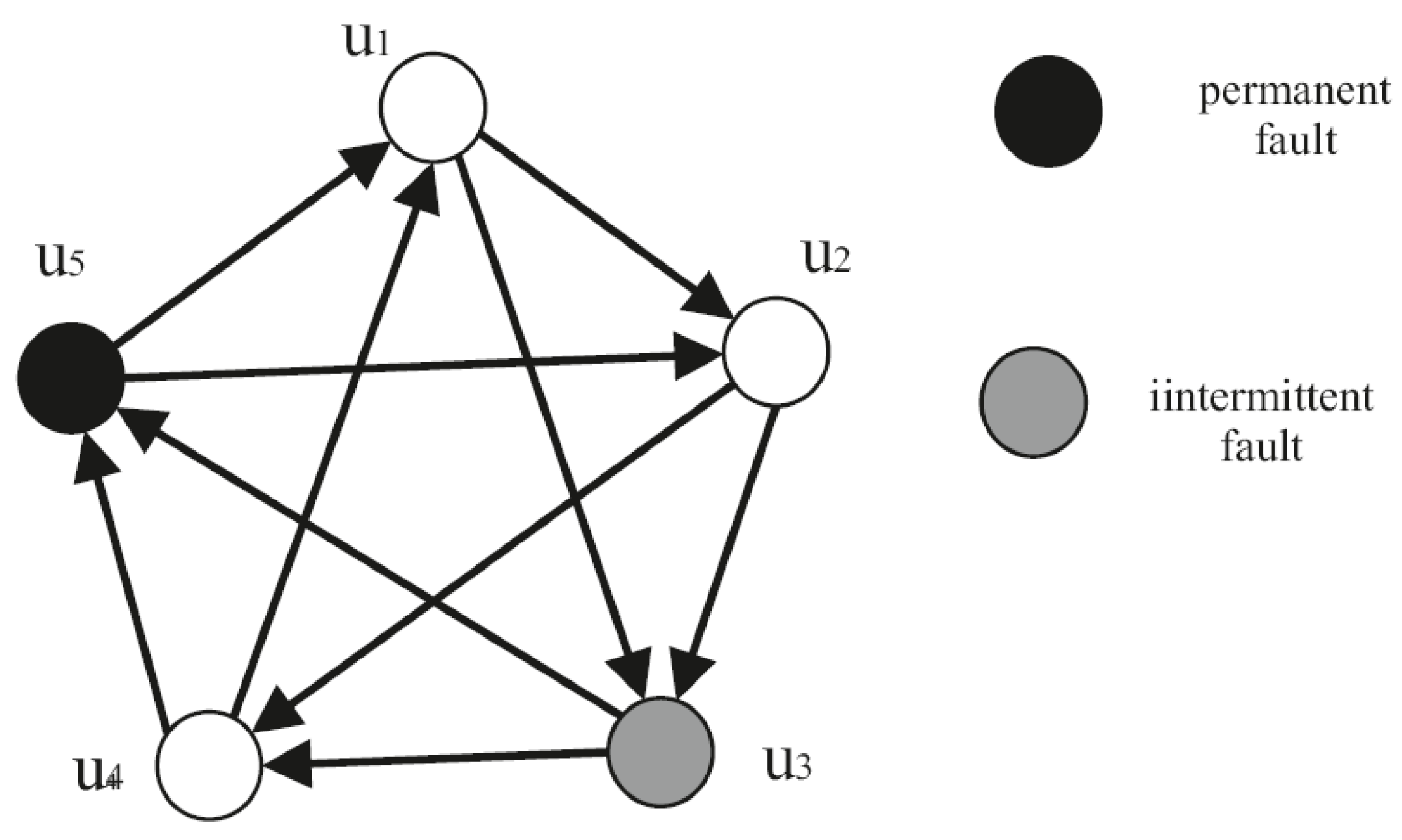
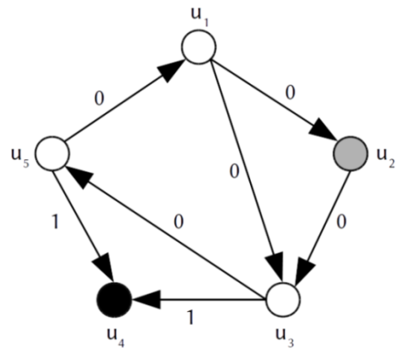
Let the system consist of five units and tests are performed according to a predefined schedule. This system is represented by the graph shown in Figure 4.
The obtained syndrome is
There exist several methods for diagnosis of permanently faulty units. Most of them make the assumption about the maximum possible number of faulty units in the system. In [22], it was proven that correct system diagnosis is possible if the total number of faulty units do not exceed the value t, where
It is easy to verify that no system state (i.e., no combination of permanently faulty and fault-free units in which the total number of permanently faulty units does not exceed the value t) can lead to obtaining such syndrome Rd.
For example, if units and are permanently faulty, result should be equal to 1, whereas in syndrome Rd this result is equal to 0.
Thus, direct application of algorithms developed for diagnosis only permanently faulty units is not possible.
Such situation can be explained by specific behavior of some faulty units. Particularly, a unit can be intermittently faulty. It means that at one moment it behaves like a permanently faulty unit, whereas at other moments like a fault-free unit.
Thus, new methods for diagnosis intermittently faulty units at system level should be developed.
5. Diagnosis of System with Intermittently Faulty Units
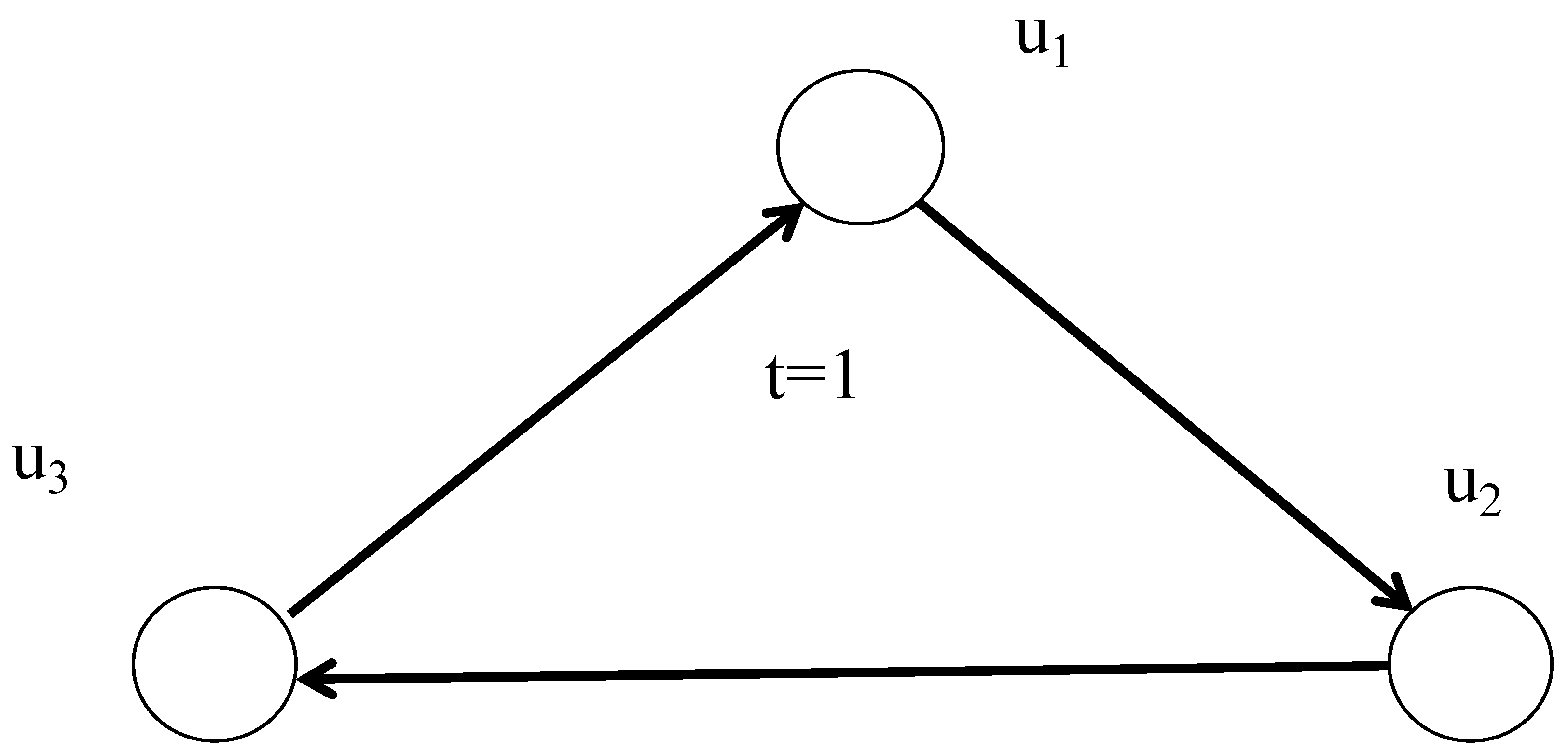
Let’s consider example when system consists of three units (as shown in Figure 5).
Such system can be correctly diagnosed if not more than one permanently faulty unit is allowed (i.e., ). The table of potential syndromes that can be obtained when only permanently faulty units can take place looks as follows:
For the considered example the following syndromes can be obtained:
These syndromes form the set , that is .
Generally, for the systems with units and with testing graphs of type the cardinality of set is equal to
Structure is the structure in which unit tests unit if and only if
where .
Now let’s consider the case when unit has intermittent fault which during test is in passive state and during test is in active state. In the given case, the following syndrome can be obtained Application of any diagnosis algorithm developed for diagnosis of systems with only permanently faulty units gives the result indicating that unit u2 is faulty. This result is incorrect.
Hence, we cannot apply these diagnosis algorithms directly for diagnosis systems when intermittent faults are allowed. For this case Mallela and Masson [8] suggested to repeat the tests several times in order to form the summary syndrome .
Summary syndrome is obtained after performing rounds of test routine (i.e., repetition of tests). Summary syndrome is computed as follows
where -syndrome obtained in -th round of repetition of test routine.
When summary syndrome is a subset of set (i.e., ), the algorithms developed for diagnosing permanently faulty units can be also used for considered faulty situation. is a set of syndromes that can be obtained when only permanently faulty units can take place (considering that number of faulty units do not exceed the maximum number of faulty units which is allowable for diagnosable system).
Getting back to the considered example, let’s assume that tests are repeated only once. Let’s also assume that intermittent fault of unit u1 during repeated test will be in active state (i.e., ). In the given case, summary syndrome takes the form
Diagnosis performed on the basis of gives the result indicating that unit is faulty. This result is correct (see Table 2).
To verify if the main condition is met, several methods can be used. For example, syndrome can be sequentially compared with every potential syndrome from set . Another method consists in the following. First element of is compared with the first elements of each syndrome from set . After this step most of syndromes can be deleted from set , particularly those in which the first element is distinct from the first element of . Then the second element of is compared with the second elements of the syndromes which remain in set . After this step further syndromes can be deleted from set , as it was done at previous step. This procedure proceeds until set contains only one syndrome which is similar to (i.e., main condition is met). Otherwise, when there is no match, the main condition is not met.
Next method assumes that set R0 can be formed in advance and for each element of whole number can be associated. For example, in the considered example potential syndrome is associated with , since . Whole number is also computed for . Then, this number is sequentially compared with the numbers of syndromes from . As soon as the match is found, the procedure of comparing is ended (i.e., main condition is met). If match is not found, main condition is not met.
For arbitrary testing graphs that are formed dynamically (when tests are performed randomly) it is not possible to perform analysis of potential syndromes in advance. For this case we propose the approach that allows solving both the task of formation of all potential syndromes and the task of verifying the main condition.
6. Formation of Potential Syndromes and Verifying the Main Condition
We consider system self-diagnosis when system units perform both system tasks and diagnosis. Diagnosis includes performing of the tests and executing of diagnosis algorithm. Since system units are restricted in resources (memory, time), it is important to simplify and reduce the number of operations performed by each system unit.
Recently some new programming languages were developed that can be used to provide implementation of system self-diagnosis. We have chosen Julia language for pilot implementation of the proposed algorithm and data structures. Julia is a high-level programming language very suitable for the presentation of ideas in the form which is relatively close to mathematical notation. On the other hand Julia supports low level constructs and hardware optimization (in reality it can the product code which is more efficient than code in C language and comparable to performance of HPC Fortran compilers). Julia is now a stable language with a growing community.
6.1. Data Representation
We suggest to performing basic operations on syndromes and on the sets of syndromes by way of utilization of bit arrays and vectorized the version of bitwise operations.
This brings two main benefits:
- Compact representation of diagnosis graphs and syndromes (allows the decrease of the memory consumption by a factor 4); and
- Full utilization of several types of hardware parallelism (including concurrency of bitwise operators).
The implementation in Julia uses high level constructs but it is available only for systems based on x86 and ARM platforms (32 bit and 64 bit). Moreover, for systems with fixed and limited numbers of units there exists the simple and effective implementation in native machine code (only basic bitwise operations are used). In the given case, application of the suggested approach for resource-restricted embedded systems is also possible and efficient (e.g., for IoT agents and their swarms). Table 3 summarizes the main characteristics of the suggested implementations.
Testing graphs of the system can be represented by the square adjacency matrix of dimension n × n, where n is the total number of units in the system. Elements of this matrix are Boolean values. (If unit ui performs a test on unit uj, the item on the i-th row and j-th column takes the value true, otherwise false). The matrix of Boolean values can be represented in packed form. In the given case, matrix items are represented by single bits and the matrix of Boolean values is represented by bit arrays.
Julia language supports bit arrays with arbitrary dimensions using standard library of data structures. Therefore, the definition of new data type for data of the adjacency matrix is straightforward.
struct TestingGraph
tests: BitArray{2} # adjacency matrix as 2D bit array
end
The system global state (vector of states of units) is represented in an external data structure (it can be modified independently from the testing graph) by means of an alias of 1D bit array (alias does not create a nominally new type but only a new identifier for an existing one). In this bit array, zero represents the faulty unit.
SystemState = BitArray{1}
Usually a syndrome is depicted in testing graph as weights of edges. In the given case, weights are results of tests. A result can take values either 0 or 1. In Figure 6, example of syndrome for the system with five units is shown.
These types of weighted graphs can be represented by a pair of Boolean matrices (in packed bit array representation). The first matrix (denoted as mask) is identical to the adjacency matrix of the testing graph as it defines the positions of valid results (i.e., the results equal to 0). The second matrix codes results of tests (true represents results equal to 0, false represents result equal to 1). Only results with true bit in the mask matrix are valid.
This somewhat counterintuitive representation of the results’ value makes some operations (e.g., membership function) more efficient.
For example the syndrome depicted in Figure 6 can be created by the following call of the constructor:
Syndrome(5, [((1,2), 0), ((1,3),0), ((2,3), 0),((3,4), 1), ((3,5), 0), ((5,1), 0), ((5,4), 1)])
struct Syndrome
mask:: BitArray{2}
results:: BitArray{2}
end
The Julia makes possible definition of auxiliary constructing functions (constructors) for initialization of complex data structures. The syndrome can be initialized from array of tuples ((checkingUnit, checkedUnit), result).
function Syndrome(n::Int, results::Vector{Tuple{Tuple{Int, Int}, Int}})
# both matrices are inicialized by falses
s = Syndrome(falses(n,n), falses(n,n))
for ((checking, checked), result) in results # for every results
s.results[checking, checked] = (result = 0) # set bit in results
s.mask[checking, checked] = true # and mask
end
returns
end
In this representation, the summary syndrome is computed by reducing (folding) the list of syndromes by binary operation of syndrome union (denoted as ). This operation is implemented by bitwise AND between results matrix of syndromes
function ∪(s1::Syndrome, s2::Syndrome)
if s1.mask! = s2.mask
throw(ArgumentError(“Incompatible syndromes”))
end
return Syndrome(s1.mask, s1.results & s2.results)
end
R_∑(syndromes::Vector{Syndrome}) = reduce(∪, syndromes)
The set of syndromes is expressed by the same internal structure as syndrome with slightly alternative meaning of bit mask. In the given case, true bit in mask is interpreted as unambiguous result of test. False bit is interpreted as ambiguous result of test (in set , it is denoted as ‘’) or non-existent test. The new type is defined for better static type checking (Julia has nominal optional static type system).
struct SyndromeSet
mask:: BitArray{2}
results::BitArray{2}
end
6.2. Testing of Membership of
The implementation of membership function which checks if a syndrome is element of some syndrome set is possible using only basic bitwise operation AND, OR and XOR (denoted as &, | and ⊻ or . & .|, . ⊻ in vectorized form in Julia).
function ∈ (s::Syndrome, s_set::SyndromeSet)
if s_set.mask & s.mask! = s_set.mask
throw(ArgumentError(“Incompatible syndrome”))
end
cover = (s_set.results v s.results) & s_set.mask
return! reduce(|, cover)
end
The implementation exploits the map-reduce approach. Here, XOR is applied between bit array of results of obtained syndrome and bit array of expected results of syndrome. Operation is performed only on valid bits of set (see mask operation by AND). Reduce step is performed by bitwise OR (any true bit leads to denial of membership).
The second step is construction of set of possible syndrome for a testing graph and a permanent global state (designed as constructor of SyndromSet structure). This code uses only AND bitwise operation and matrix transposition (denoted by ′ operator which performs matrix conjugate transformation)
SyndromeSet(tg::TestingGraph, state::SystemState)=SyndromeSet(tg.tests & state, tg.tests & state’)
The mask array of set is constructed by vector application of bitwise AND between adjacency matrix of testing graph and column vector of unit’s states. That is, operation AND is applied on rows (because validity of testing is determined by testing unit). The result array of set is outcome of application of transposed vector of unit’s states and adjacency matrix (operation AND is applied on columns because results of testing are determined by tested unit).
The set is constructible by mean of iteration over each possible diagnosable state of system, which can be generated from binary form of numbers between an with maximum of zeros (where is maximal -diagnosability).
function R_0(tg::TestingGraph)
n = size(tg)
t = (n − 1) ÷ 2
return [SyndromeSet(tg, state)
for state
in (SystemState(digits(i, base = 2, pad = n)) for i = 2^n − 1:−1:0)
ifn-count(state) ≤ t]
end
The function uses array comprehensions which iterate over bit arrays constructed from binary digits (the better iterators over required bit permutations can be used, but are much more complicated). The count function returns numbers of 1 s in bit array.
With this preparation the trivial implementation of checking, if syndrome is a member of set is straightforward.
Any (R_∑(list_of_syndromes) ∈ set in R_0(dg))
The more optimal checking can use partial order between sets in and exclude some syndromes from .
7. The Case When the Main Condition is Not Met
For diagnosis of intermittent faults it is important to determine the number of test routine repetitions, . It is also needed to determine what should be done if after repetitions the condition is not satisfied.
To solve these tasks, we suggest the following decision. It is suggested to repeat the test routine several times, . Concrete number of repetitions of test routine depends on the total number of units in the system N, on the classes of intermittent faults, which are going to be detected, and on the required credibility of diagnosis. If an intermittent fault belongs to class 4, the value of does not influence the test results. If an intermittent fault belongs to class 3, a unit with such fault behaves either as fault-free or as faulty only during one test. Any next test will show that this unit behaves as fault-free. Thus, two tests are sufficient to form which make condition true. It also concerns an intermittent fault of class . In case 2, a unit with such intermittent fault with high probability will behave as permanently faulty. There is low probability that one of the tests will show that this unit is fault-free. Although, any other test will show that this unit is faulty. Thus, two tests are enough to form syndrome , which satisfies the condition mentioned above.
If after several rounds of tests repetitions the condition is not true, then it is needed to determine a consistent set of units, . Set contains all of the units that, according to the summary syndrome, are diagnosed as fault-free. Units that belong to the set evaluate each other as fault-free. In order to determine the set , it is needed to remove from summary syndrome all test results which are equal to 1. Remaining results allow to form a Z-graph.
Z-graph is formed as follows. If in is equal to 0, then there is an edge between vertices and in Z-graph directed from to .
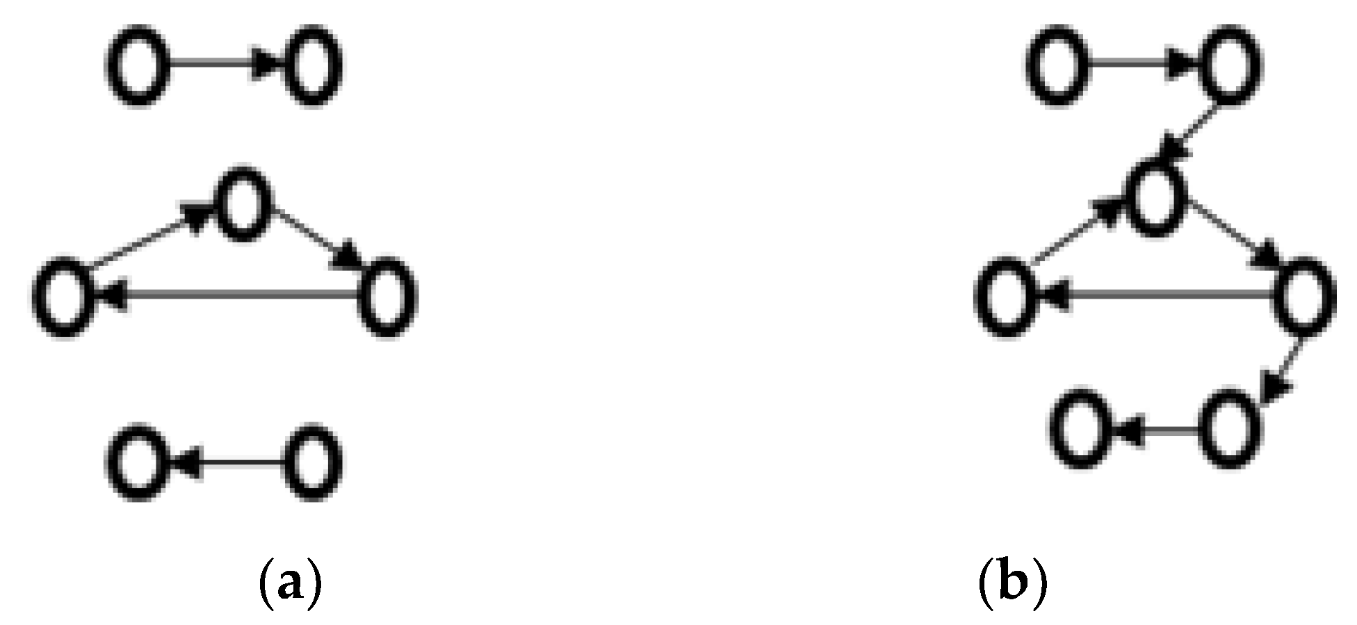
Credibility of diagnosis result will be greater when Z-graph is connected [26]. In Figure 7, examples for connected and disconnected Z-graphs are shown.
Connection of Z-graphs depend considerably on the testing assignment and on the allowed number of faulty units (i.e., on the maximum number of faulty units that still allow the obtaining of the correct result of diagnosis).
We consider the case when tests among system units are performed in accordance with a pre-set schedule (i.e., defined a priori). Having the testing graph, it is possible to investigate if Z-graph is connected under the condition whereby the maximum number of faulty units does not exceed value t.
Since each edge of the graph involves two vertices, the minimal number of edges which still allows for the providing of system t-diagnosability [26], , is equal to
Next, we can examine if the value Lmin is sufficient in order that the Z-graph be connected.
Given Lmin, we can determine the minimal number of edges in the Z-graph, Kmin, that ensures connection among its vertices. Kmin can be determined as follows
The Z-graph is connected if
This inequality is true for (that is, when the total number of system units is less than seven).
In the case when N ≥ 7, value Lmin is not sufficient in order for Z-graph be connected. In the given case, we can determine the number of additional edges that must be added to the Z-graph in order that for graph to become connected.
Using results presented in [18], it is possible to conclude that the Z-graph maximally may have
components each of which consists either of two vertices for , or of two vertices except the one consisting of three vertices for .
In order to connect these components additional edges are necessary. The choice of the pair of units for performing a test that corresponds to the additional edge in Z-graph can be carried out according to existing algorithms [26].
For Z-graph it is possible to form the matrix MR. Matrix MR is square matrix presentation of the subset of which has only zero results. If result is an element of the resulting subset of , then element of matrix has value of 0. Otherwise, element is denoted as dash.
There could be used the diagnosis algorithm presented in. This algorithm is based on the matrix which is similar to matrix and can identify all faulty units (on the condition that total number of faulty units does not exceed the value ). Handling matrices like is also presented in.
In the given case, it is needed to calculate the total number of 0 in each column. Then, obtained numbers , should be compared with value t. If , then unit is diagnosed as fault-free. If condition is not true for all then it is needed to find in Z-graph a simple directed cycle of length . Such cycle can be determined from matrix . All units, which are in this cycle, should be identified as fault-free.
Units that are not identified as fault-free are either permanently faulty or have an intermittent fault. It should be noted that there is low probability of incorrect diagnosis. This probability can be evaluated in relation to different total number of system units, different classes of intermittent faults and different number of test routine repetitions [24].
The task of determining the probability of diagnosis results (fault omission and incorrect identification of fault-free units) is a separate task and it was not the subject of this paper.
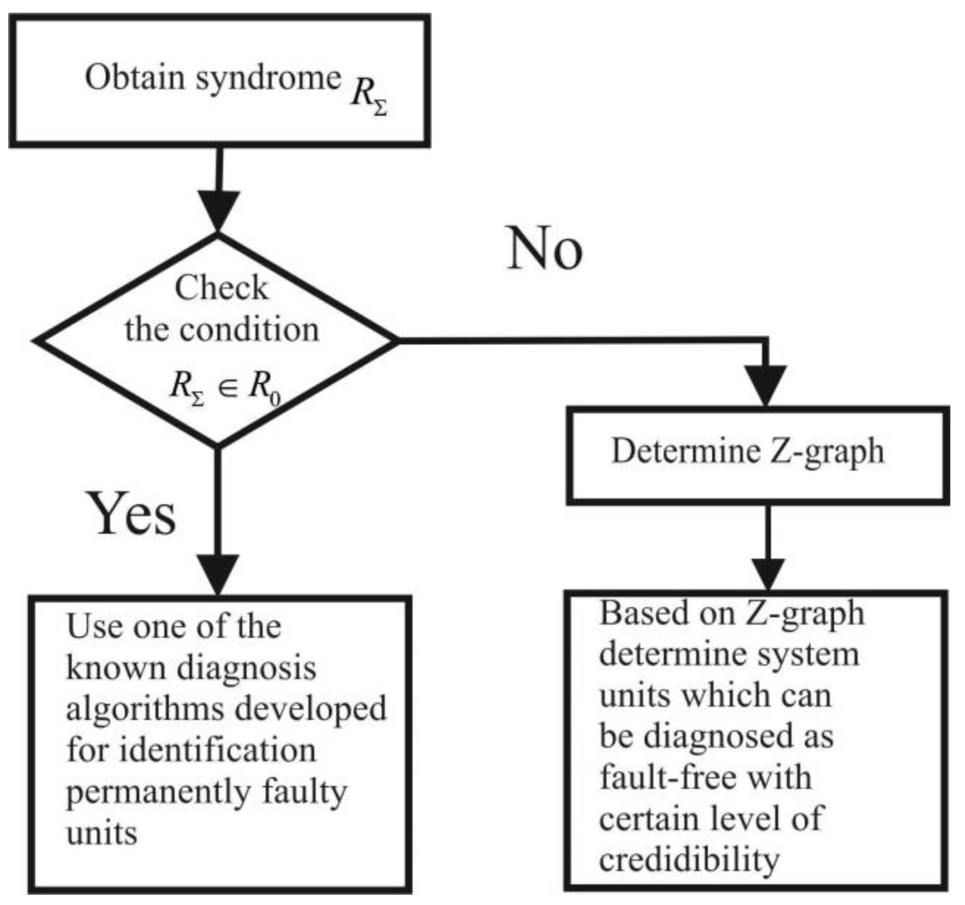
Figure 8 summarizes the presented approach to diagnosis at a system level when units can be intermittently faulty.
8. Conclusions
System level diagnosis is an abstraction at a high level and, thus, its practical implementation to particular cases of complex systems is the task which requires additional investigations, both theoretical and modeling. Mostly, system level self-diagnosis deals with the diagnosis of permanently faulty units. Although, there are many real situations when intermittently faulty units can occur in the system. In the given case it is necessary to take into account various behaviors of such faulty units.
Behavior of intermittent faults can be modeled by continuous Markov chain with two states—Passive (PS) and Active (AS). If an intermittent fault is in PS, unit acts as fault-free. If an intermittent fault is in an AS, the unit acts as faulty (i.e., as if it has a permanent fault).
During system level self-diagnosis both permanent and intermittent faults can occur. Each test evaluates the state of a unit either as fault-free or as faulty. In the latter case, it does not discriminate the permanent and intermittent faults.
Diagnosis algorithms that deal with the sets of test results can consider (take into account) the testing time and, thus, potentially they could discriminate the permanent and intermittent faults. For this, the testing procedure must be very long. In reality, it is needed to perform the testing procedure in acceptable time for each concrete system. This leads to the situation when it is very difficult to discriminate between permanent and intermittent faults. In view of this, we are not going to provide discrimination between permanently and intermittently faulty units. All units that are not diagnosed as fault-free should be considered as faulty without further specification.
In the paper, we follow the approach to diagnose intermittent faults suggested by Mallela and Masson. That is, we provide diagnosis based on the summary syndrome. Implementation of such diagnosis requires formation of potential syndromes and verification of conditions introduced by Mallela and Masson. These tasks can be easily performed for the cases where tests are performed according to predefined schedule. In this paper, we considered more complex case when tests can be performed randomly and the testing graph is arbitrary. We also extended the diagnosis algorithm so that now it could cope with the situation when the main condition was not met.
One of the main advantages of our proposed approach to diagnose complex systems consists of its applicability during system operation. In the given case, system units perform both system tasks and diagnosis. After recovery from faults, system diagnosis proceeds using the same diagnosis algorithm.
Author Contributions
V.M. and J.F. performed the approbations. V.L. and M.V. Wrote the manuscript with input from all authors. V.M. and V.L. contributed to the final version of the manuscript.
Funding
This research received no external funding.
Conflicts of Interest
The authors declare no conflict of interest.
References
- Gepner, P.; Kowalik, M. Multi-Core Processors: New Way to Achieve High System Performance. In Proceedings of the International Symposium on Parallel Computing in Electrical Engineering (PARELEC’06), Bialystok, Poland, 13–17 September 2006. [Google Scholar] [CrossRef]
- Avizienis, A.; Laprie, J.C.; Randell, B. Dependability and its threats. A Taxonomy. In Proceedings of the IFIP 18th World Computer Congress “Building the Information Society”, Toulouse, France, 22–27 August 2004; pp. 91–120. [Google Scholar]
- Psarakis, M.; Gizopoulos, D.; Sanchez, E.; Sonza Reorda, M. Microprocessor Software-Based Self-Testing. IEEE Des. Test Comput. 2010, 27, 4–19. [Google Scholar] [CrossRef]
- Mashkov, V. Task Allocation among Agents of Restricted Alliance. In Proceedings of the IASTED ISC’2005 Conference, Cambridge, MA, USA, 31October–2 November 2005; pp. 13–18. [Google Scholar]
- Mashkov, V. Restricted alliance and coalition formation. In Proceedings of the IEEE/WIC/ACM International Conference on Intelligent Agent Technology, Beijing, China, 24 September 2004; pp. 329–332. [Google Scholar]
- Mashkov, V.A.; Barabash, O.V. Self-checking of modular systems under random performance of elementary checks. Eng. Simul. 1995, 12, 433–445. [Google Scholar]
- Mashkov, V.; Barabash, O. Self-checking and self-diagnosis of module systems on the principle of walking diagnostic kernel. Eng. Simul. 1998, 15, 43–51. [Google Scholar]
- Mallela, S.; Masson, G. Diagnosable systems for intermittent faults. IEEE Trans. Comput. 1978, 27, 560–566. [Google Scholar] [CrossRef]
- Tang, Q.; Chai, Y.; Qu, J.; Fisher, R.H. Discriminative Sparse Representation Based on DBN for Fault Diagnosis of Complex System. Appl. Sci. 2018, 8, 795. [Google Scholar] [CrossRef]
- Xiao, Y.; Hong, Y.; Chen, X.; Chen, W. The Application of Dual-Tree Complex Wavelet Transform (DTCWT) Energy Entropy in Misalignment Fault Diagnosis of Doubly-Fed Wind Turbine (DFWT). Entropy 2017, 19, 587. [Google Scholar] [CrossRef]
- Wei, Y.; Yue, Y. Research on Fault Diagnosis of a Marine Fuel System Based on the SaDE-ELM Algorithm. Algorithms 2018, 11, 82. [Google Scholar] [CrossRef]
- Ntalampiras, S. Fault Identification in Distributed Sensor Networks Based on Universal Probabilistic Modeling. IEEE Trans. Neural Netw. Learn. Syst. 2014, 1939–1949. [Google Scholar] [CrossRef] [PubMed]
- Ntalampiras, S. Fault Diagnosis for Smart Grids in Pragmatic Conditions. IEEE Trans. Smart Grids 2016, 1964–1971. [Google Scholar] [CrossRef]
- Syed, W.A.; Khan, S.; Phillips, P.; Perinpanayagam, S. Intermittent fault finding strategies. Procedia CIRP 2013, 11, 74–79. [Google Scholar] [CrossRef]
- Ahmad, W.S.; Perinpanayagam, S.; Jennions, I.; Khan, S. Study on intermittent faults and electrical continuity. Procedia CIRP 2014, 22, 71–75. [Google Scholar] [CrossRef]
- Chen, J.; Kher, S.; Somani, A. Distributed fault detection of wireless sensor network. In Proceedings of the International Conference on Mobile Computing and Networking, New York, NY, USA, 26 September 2006; pp. 65–72. [Google Scholar]
- Jangale, S.; Hadsul, D. Detection of faulty sensor nodes in wireless sensor network. Comput. Technol. Appl. 2013, 4, 150–154. [Google Scholar]
- Jiang, P. A new method for fault detection in wireless sensor networks. Sensors 2009, 9, 1282–1294. [Google Scholar] [CrossRef] [PubMed]
- Lee, M.H.; Choi, Y.H. Fault detection on wireless sensor networks. Comput. Commun. 2008, 31. [Google Scholar] [CrossRef]
- Albini, L.; Duarte, J.; Ziwich, R. A generalized model for distributed comparison-based system-level diagnosis. J. Braz. Comput. Soc. 2005, 10, 44–56. [Google Scholar] [CrossRef] [Green Version]
- Chessa, S.; Santi, P. Comparison-based system-level fault diagnosis in ad hoc network. In Proceedings of the 20th Symp. Reliable Distributed Systems, New Orleans, LA, USA, 31 October 2001; pp. 257–266. [Google Scholar]
- Gevorkyan, M.N.; Korolkova, A.V.; Kulyabov, D.S.; Lovetskyi, K.P. Statistically Significant Comparative Performance Testing of Julia and Fortran Languages in Case of RungeKutta Methods. In Proceedings of the Numerical Methods and Applications: 9th International Conference, NMA 2018, Borovets, Bulgaria, 20–24 August 2018; Revised Selected Papers. Springer: Berlin, Germany, 2019; pp. 400–407. [Google Scholar]
- Kamal, S.; Page, C.V. Intermittent fault: A model and a detection procedure. IEEE Trans. Comput. 1974, 23, 713–719. [Google Scholar] [CrossRef]
- Mashkov, V.; Fiser, J.; Lytvynenko, V.; Voronenko, M. Self-diagnosis of the systems with intermittently faulty units. In Proceedings of the 2018 IEEE Second International Conference on Data Stream Mining and Processing, Lviv, Ukraine, 21–25 August 2018; pp. 411–414. [Google Scholar]
- Preparata, T.; Metze, G.; Chien, R. On the connection assignment problem of diagnosable system. IEEE Trans. Electron. Comput. 1967, 16, 848–854. [Google Scholar] [CrossRef]
- Mashkov, V.; Pokorny, J. Scheme for comparing results of diverse software versions. In Proceedings of the ICSOFT Conference, Barcelona, Spain, 22–25 July 2007; pp. 341–344. [Google Scholar]
Figure 1.
Model of intermittent fault.

Figure 2.
Example of testing graph.

Figure 3.
Different behaviors of intermittent faults.

Figure 4.
Testing graph for the considered system.

Figure 5.
Testing graph of a system.

Figure 6.
Instance of syndrome for testing graph.

Figure 7.
Examples of Z-graph. (a) Z-graph is disconnected; (b) Z-graph is connected.

Figure 8.
Diagnosis of system units when intermittent faults are allowed.


Table 1.
Various types of intermittent faults.
| Ratio ttesting/A | A = 1/λ | A = 1/μ |
|---|---|---|
| case 1 (class 1) | large | large |
| case 2 (class 2) | large | small |
| case 3 (class 3) | small | large |
| case 4 (class 4) | small | small |
Table 2.
Table of potential syndromes.
| System State | Syndrome | ||
|---|---|---|---|
| S0: all units are fault-free | 0 | 0 | 0 |
| S1: unit u1 is faulty | either 0 or 1 | 0 | 1 |
| S2: unit u2 is faulty | 1 | either 0 or 1 | 0 |
| S3: unit u3 is faulty | 0 | 1 | either 0 or 1 |
Table 3.
Characteristics of code implementation.
| Implementation | Target Platform | Paralellism | Maximal Number of Units in System | Memory Consumption | Count of Arithmetic Instruction for Testing the Condition |
|---|---|---|---|---|---|
| classical array implementation (in C or Fortran) | desktop and some embedded system | only on compilers with vectorization support (e.g., OpenMP 3.0 with SIMD) | unlimited | bytes | 2 |
| Julia bit arrays | ARM, x86 (32 and 64 bits) | SIMD (SSE, NEON) bit operation | unlimited | 2 bites = /4 bytes + rounded up to machine word + alignment (critical for SIMD systems) | / 128 (for x86 AVX) + better locality of CPU caches |
| assembler code | embedded system microcontrollers (8–32 bits) | bit operation | width of universal registers (8–32) | 2 bites = /4 bytes | / 8 (for 16 bit systems) + better locality of CPU caches |
© 2019 by the authors. Licensee MDPI, Basel, Switzerland. This article is an open access article distributed under the terms and conditions of the Creative Commons Attribution (CC BY) license (http://creativecommons.org/licenses/by/4.0/).
Share and Cite
MDPI and ACS Style
Mashkov, V.; Fiser, J.; Lytvynenko, V.; Voronenko, M. Diagnosis of Intermittently Faulty Units at System Level. Data 2019, 4, 44. https://0-doi-org.brum.beds.ac.uk/10.3390/data4010044
AMA Style
Mashkov V, Fiser J, Lytvynenko V, Voronenko M. Diagnosis of Intermittently Faulty Units at System Level. Data. 2019; 4(1):44. https://0-doi-org.brum.beds.ac.uk/10.3390/data4010044
Chicago/Turabian StyleMashkov, Viktor, Jirí Fiser, Volodymyr Lytvynenko, and Maria Voronenko. 2019. "Diagnosis of Intermittently Faulty Units at System Level" Data 4, no. 1: 44. https://0-doi-org.brum.beds.ac.uk/10.3390/data4010044